AUTOENCODER BASED IMAGE COMPRESSION: CAN THE LEARNING BE QUANTIZATION INDEPENDENT?
Abstract
This paper explores the problem of learning transforms for image compression via autoencoders. Usually, the rate-distortion performances of image compression are tuned by varying the quantization step size. In the case of autoencoders, this in principle would require learning one transform per rate-distortion point at a given quantization step size. Here, we show that comparable performances can be obtained with a unique learned transform. The different rate-distortion points are then reached by varying the quantization step size at test time. This approach saves a lot of training time.
Index Terms— Image compression, deep autoencoders, quantization.
1 Introduction
Image coding standards all use linear and invertible transforms to convert an image into coefficients with low statistical dependencies, i.e suited for scalar quantization. Notably, the discrete cosine transform (DCT) is the most commonly used for two reasons: it is image-independent, implying that the DCT does not need to be transmitted, it approaches the optimal orthogonal transform in terms of rate-distortion, assuming that natural images can be modeled by zero-mean Gaussian-Markov processes with high correlation [1]. Deep autoencoders have been shown as promising tools for finding alternative transforms [2, 3, 4]. Autoencoders learn the encoder-decoder non-linear transform from natural images.
In the best image compression algorithms based on autoencoders [5, 6, 7], one transform is learned per rate-distortion point at a given quantization step size. Then, the quantization step size remains unchanged at test time so that the training and test conditions are identical. By contrast, image coding standards implement adaptive quantizations [8, 9]. Should the quantization be imposed during the training? To answer this, we propose an approach where the transform and the quantization are learned jointly. Then, we investigate whether, at test time, the compression falls apart when the coefficients obtained with the learned transform are quantized using quantization step sizes which differ from those in the training stage. The code to reproduce our numerical results and train the autoencoders is available online111www.irisa.fr/temics/demos/visualization_ae/visualizationAE.htm .
Matrices and tensors are denoted by bold letters. is the Frobenius norm of . is the elementwise multiplication between and .
2 Joint learning of the transform and the quantization
Section 2 introduces an efficient autoencoder for image compression. Then, it details our proposal for learning jointly this autoencoder transform and the quantization.
2.1 Autoencoder for image compression
An autoencoder is a neural network with an encoder , parametrized by , that computes a representation from the data , and a decoder , parametrized by , that gives a reconstruction of , see Figure 1. Autoencoders can be used for denoising or dimensionality reduction. When it is used for compression, the representation is also quantized, leading to the new quantized representation . If an autoencoder has fully-connected layers [10, 11, 12], the number of parameters depends on the image size. This implies that one autoencoder has to be trained per image size. To avoid this, an architecture without fully-connected layer is chosen. It exclusively comprises convolutional layers and non-linear operators. In this case, is a set of feature maps of size , see Figure 1.

The basic autoencoder training minimizes the image reconstruction error [13]. In order to create a rate-distortion optimization, the authors in [6] add the minimization of the entropy of the quantized representation. Moreover, a bit allocation is performed by learning a normalization for each feature map of . The encoder followed by the normalizations at the encoder side, parametrized by , are denoted . Similarly, the normalizations at the decoder side, parametrized by , followed by the decoder are denoted . Finally, this leads to (2.1).
| (1) |
is the probability mass function of the quantized feature map coefficients . The expectation is approximated by averaging over a training set of images. Unfortunately, makes minimization (2.1) unusable. Indeed, the derivative of any quantization with respect to its input is at any point. Consequently, and cannot be learned via gradient-based methods [14]. To get around this issue, [6] fixes the quantization step size to 1 and approximates the uniform scalar quantization with the addition of a uniform noise of support [-0.5, 0.5]. Note that, even though the quantization step size is fixed, the bit allocation varies over the different feature maps via the normalizations. In the next section, we consider instead to remove the normalizations and learn explicitly the quantization step size for each feature map of .
2.2 Learning the quantization step sizes
We address the problem of optimizing the quantization step size for each feature map of . Because of the quantization, the function to be minimized is an implicit function of the quantization step sizes . The target is to make it an explicit function of . For ,
| (2) |
where is the probability density function of the feature map coefficients and denotes the probability density function of the continuous uniform distribution of support . The normalizations are removed from (2.1) and, using (2), (2.1) becomes (3).
| (3) | ||||
The matrix of contains realizations of , being a continuous random variable of probability density function . In (3), the function to be minimized is differentiable with respect to . can thus be learned via gradient-based methods. However, cannot yet be learned as the function to be minimized in (3) is not differentiable with respect to . This is resolved using the change of variable where is a random variable following the continuous uniform distribution of support . Now, the minimization over is feasible, see .
| (4) |
The matrix of contains realizations of . All the coefficients in the matrix of are equal to . A detail has been left out so far: is unknown. In a similar manner to [5, 6], can be replaced by a function , parametrized by , and is learned such that fits .
In the end, we end up with three groups of parameters: , , and . These three groups are learned by alternating three different stochastic gradient descents. All the training heuristics are detailed in the code1.
Section 2 has developped an approach for learning explictly the transform and a quantization step size for each feature map of . Before evaluating this approach in Section 4, Section 3 studies what would happen if, at test time, the coefficients in are quantized using quantization step sizes that differ from those in the training stage. This first requires understanding the internal structure of after the training.
3 Inside the learned representation
This section studies the different feature maps of after the training. To this end, a deep convolutional autoencoder must first be built and trained. is the composition of a convolutional layer, a generalized divisive normalization (GDN) [15], a convolutional layer, a GDN and a convolutional layer. is the reverse composition, replacing each GDN with an inverse generalized divisive normalization (IGDN) [15] and each convolutional layer with a transpose convolutional layer [16]. It is important to stress that , has one channel and the convolutional strides and paddings are chosen such that and are 16 times smaller than respectively the height and the width of . Therefore, the number of pixels in is twice the number of coefficients in . The training set contains luminance images of size that are extracted from ImageNet [17]. The minimization is (2.2), . Note that, if a GDN was placed immediately after , a IGDN was placed immediately before and, was not learned, the autoencoder architecture and the training would correspond to [6].
3.1 Distribution of the learned representation
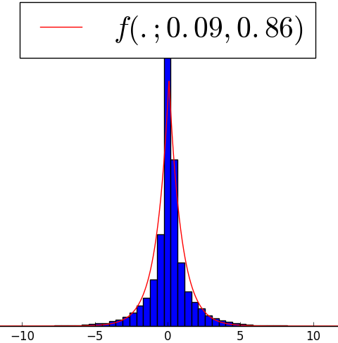
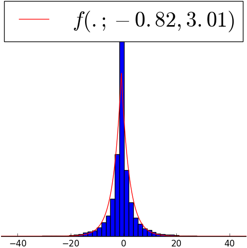
After the training, a test set of luminance images of size is created from the Kodak suite222r0k.us/graphics/kodak/. Here, refers to a test luminance image. Figure 2 shows the normed histogram of the feature map of and that of its feature map, averaged over the test set. Every feature map of , except the , has a normed histogram similar to those displayed. To be more precise, let’s write the probability density function of the Laplace distribution with mean and scale , denoted .
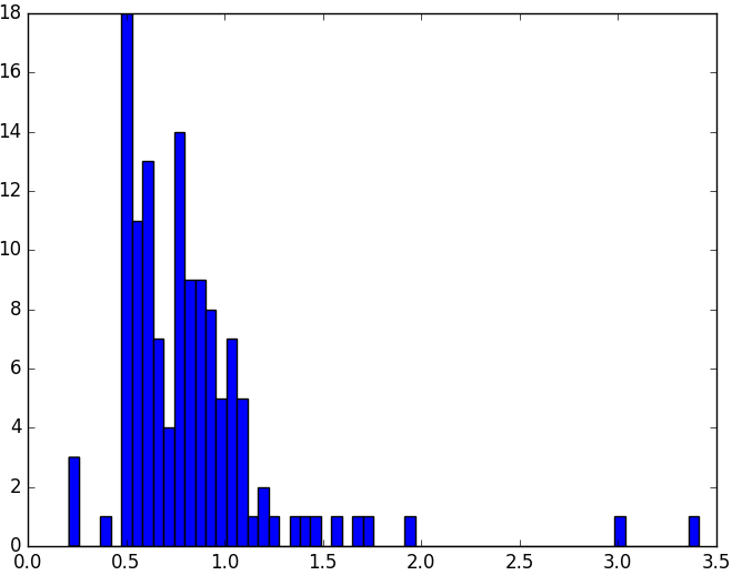
, , there exists and such that fits well the normed histogram of the feature map of . Note that most of the scales belong to , see Figure 3. For transformed coefficients having a zero-mean Laplace distribution, [18] proves that a uniform reconstruction quantizer (URQ) with constant decision offsets approaches the optimal scalar quantizer in terms of squared-error distortion for any quantization step size. Yet, in our case, the Laplace probability density functions are not zero-mean, uniform scalar quantizers are used instead of this URQ. The point is not problematic as an extra set of luminance images is used to compute an approximation of the mean of the feature map of , then, at test time, the feature map of is centered via before being quantized. Note that does not depend on the test luminance images, thus incurring no transmission cost. Regarding the point , it must be noted that the decoder mapping of the URQ is exactly the decoder mapping of the uniform scalar quantization with same quantization step size. Since our case comes close to the requirements of the proof in [18], at test time, the rate-distortion trade-off should not collapse as the quantization step sizes deviate from the learned values. This will be verified in Section 4.
3.2 Internal structure of the learned representation




The shortcoming of the previous fitting is that it does not reveal what information each matrix of encodes. To discover it, further visualizations are needed. The most common way of exploring a deep convolutional neural network (CNN) trained for image recognition is to look at the image, at the CNN input, resulting from the maximization over its pixels of a given neural activation in the CNN [19, 20, 21]. Precisely, [19, 20] maximize over the image pixels a given neural activation at the CNN output, i.e a class probability. This shows what image features characterize this class according to the CNN. In our case, the maximization over the image pixels of a given coefficient in does not yield interpretable images. Indeed, the coefficients in are not bounded. This may explain why the maximization often returns saturated images.
Alternatively, the information the feature map of encodes, , can be seen as follows. , all the coefficients in the feature map of are set to . This way, the feature maps of contains no significant information. Then, a single coefficient in the feature map of is set to and is displayed. is selected such that it is near one of the two tails of the Laplace distribution of the feature map of . Figure 4 shows the crop at the top-left of when the single coefficient is located at the top-left corner of the feature map of , . We see that the feature map of encodes a spatially localized image feature whereas its feature map encodes a spatially extended image feature. Moreover, the image feature is turned into its symmetrical feature, with respect to the mean pixel intensity, by moving from the right tail of the Laplace distribution of the feature map of to the left tail. This linear behaviour is observed for each feature map of .
4 Experiments
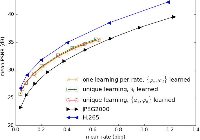
We now evaluate in terms of rate-distortion performances: whether the way of learning the quantization matters, whether, at test time, it is efficient to quantize the coefficients obtained with the learned transform using quantization step sizes which differ from those in the training stage. This is done by comparing three cases.
The case follows the approach in [6]. One transform is learned per rate-distortion point, the bit allocation being learned via the normalizations. In details, an autoencoder is trained for each , . During the training and at test time, the quantization step size is fixed to 1.0.
In the case, a unique transform is learned, the bit allocation being done by learning a quantization step size per feature map. More precisely, a single autoencoder is trained for and is learned, see Section 2. At test time, the rate varies as the quantization step sizes are equal to the learned quantization step sizes multiplied by .
In the case, a unique transform is learned, the bit allocation being learned via the normalizations. In details, a single autoencoder is trained for and, during the training, the quantization step size is 1.0. At test time, the rate varies as the quantization step size spans .
In the case, the autoencoder has the architecture described at the beginning of Section 3. In the and case, a GDN is also placed after and a IGDN is placed before . The autoencoders are trained on luminance images of size that are extracted from ImageNet. Then, at test time, the luminance images from the Kodak suite are inserted into the autoencoders. The rate is estimated via the empirical entropy of the quantized coefficients, assuming that the quantized coefficients are i.i.d. Note that, for the and the case, we have also implemented a binarizer and a binary arithmetic coder to compress the quantized coefficients losslessly, see the code1. The difference between the estimated rate and the exact rate via the lossless coding is always smaller than bbp. Figure 5 shows the rate-distortion curves averaged over the luminance images. The JPEG2000 curve is obtained using ImageMagick. The H.265 [22] curve is computed via the version HM-16.15. There is hardly any difference between the and the case. This means that the explicit learning of the transform and the quantization step sizes is equivalent to learning the transform and the normalizations while the quantization step size is imposed. Note that, in the case, the learning of involves parameters whereas, in the case, that of involves parameters. The and the case perform as well as the case. The minimization (2.2) and the training in [6] provide learned transforms which can be used with various quantization step sizes at test time. It is convenient not to train one autoencoder per compression rate as a single training takes 4 days on a NVIDIA GTX 1080. Finally, we see that the learned transforms yield better rate-distortion performances than JPEG2000. The quality of image reconstruction for the experiment in Figure 5 and another experiment on luminance images created from the BSDS300 [23] can be seen online1.
5 Conclusion
Using a unique transform learned via autoencoders and various quantization step sizes at test time, it is possible to compress as well as when learning one transform per rate-distortion point at a given quantization step size. Moreover, the learned transformed outperform other image compression algorithms based on transforms.
References
- [1] Thomas Wiegand and Heiko Schwarz, “Source coding: part I of fundamentals of source and video coding,” Foundations and Trends in Signal Processing, vol. 4 (1-2), pp. 1–222, January 2011.
- [2] George Toderici, Sean M. O’Malley, Sung Jin Hwang, Damien Vincent, David Minnen, Shumeet Baluja, Michele Covell, and Rahul Sukthankar, “Variable rate image compression with recurrent neural networks,” in ICLR, 2016.
- [3] Karol Gregor, Frederic Besse, Danilo J. Rezende, Ivo Danihelka, and Daan Wierstra, “Towards conceptual compression,” arXiv preprint arXiv:1604.08772, April 2016.
- [4] Thierry Dumas, Aline Roumy, and Christine Guillemot, “Image compression with stochastic winner-take-all auto-encoder,” in ICASSP, 2017.
- [5] Lucas Theis, Wenzhe Shi, Andrew Cunningham, and Ferenc Huszár, “Lossy image compression with compressive autoencoders,” in ICLR, 2017.
- [6] Johannes Ballé, Valero Laparra, and Eero P. Simoncelli, “End-to-end optimized image compression,” in ICLR, 2017.
- [7] Oren Rippel and Lubomir Bourdev, “Real-time adaptive image compression,” in ICML, 2017.
- [8] Michael W. Marcelli, Margaret A. Lepley, Ali Bilgin, Thomas J. Flohr, Troy T. Chinen, and James H. Kasner, “An overview of quantization in JPEG 2000,” Image Communication, vol. 17 (1), pp. 73–84, January 2002.
- [9] Thomas Wiegand and Heiko Schwarz, “Video coding : part II of fundamentals of source and video coding,” Foundations and Trends in Signal Processing, vol. 10 (1-3), pp. 1–346, December 2016.
- [10] Ruslan R. Salakhutdinov and Geoffrey E. Hinton, “Semantic hashing,” in SIGIR Workshop on Information Retrieval and Applications of Graphical Models, 2007.
- [11] L. Deng, M. Seltzer, D. Yu, A. Acero, A. Mohamed, and G. Hinton, “Binary coding of speech spectrograms using a deep auto-encoder,” in INTERSPEECH, 2010.
- [12] Alex Krizhevsky and Geoffrey E. Hinton, “Using very deep autoencoders for content-based image retrieval,” in ESANN, 2011.
- [13] Yoshua Bengio, “Learning deep architectures for AI,” Foundations and Trends in Machine Learning, vol. 2 (1), pp. 1–127, 2009.
- [14] David E. Rumelhart, Geoffrey E. Hinton, and Ronald J. Williams, “Learning representations by back-propagating errors,” Nature, vol. 323, pp. 533–536, October 1986.
- [15] Johannes Ballé, Valero Laparra, and Eero P. Simoncelli, “Density modeling of images using a generalized normalization transform,” in ICLR, 2016.
- [16] Vincent Dumoulin and Francesco Visin, “A guide to convolution arithmetic for deep learning,” arXiv preprint arXiv:1603.07285, March 2016.
- [17] Jia Deng, Wei Dong, Richard Socher, Li-Jia Li, Kai Li, and Fei-Fei Li, “ImageNet: a large-scale hierarchical image database,” in CVPR, 2009.
- [18] Gary J. Sullivan, “Efficient scalar quantization of exponential and laplacian random variables,” IEEE Transactions on Information Theory, vol. 42, pp. 1365–1374, September 1996.
- [19] Karen Simonyan, Andrea Vedaldi, and Andrew Zisserman, “Deep inside convolutional networks: visualizing image classification models and saliency maps,” in ICLR, 2014.
- [20] Anh Nguyen, Jason Yosinki, and Jeff Clune, “Deep neural networks are easily fooled: high confidence predictions for unrecognizable images,” in CVPR, 2015.
- [21] Jason Yosinski, Jeff Clune, Anh Nguyen, Thomas Fuchs, and Hod Lipson, “Understanding neural networks through deep visualization,” in ICML, 2015.
- [22] Gary J. Sullivan, Jens-Rainer Ohm, Woo-Jin Han, and Thomas Wiegand, “Overview of the High Efficiency Video Coding (HEVC) Standard,” IEEE Transactions on Circuits and Systems for Video Technology, vol. 22 (12), pp. 1649–1667, December 2012.
- [23] David Martin, Charless Fowlkes, Doron Tal, and Jitendra Malik, “A database of human segmented natural images and its application to evaluating segmentation algorithms and measuring ecological statistics,” in Proc. Int’l Conf. Computer Vision, 2001.