High order time integrators for the simulation of charged particle motion in magnetic quadrupoles

Abele Simona (1), Luca Bonaventura(1)
Thomas Pugnat (2), Barbara Dalena (2)
Abstract

Magnetic quadrupoles are essential components of particle accelerators like the Large Hadron Collider. In order to study numerically the stability of the particle beam crossing a quadrupole, a large number of particle revolutions in the accelerator must be simulated, thus leading to the necessity to preserve numerically invariants of motion over a long time interval and to a substantial computational cost, mostly related to the repeated evaluation of the magnetic vector potential. In this paper, in order to reduce this cost, we first consider a specific gauge transformation that allows to reduce significantly the number of vector potential evaluations. We then analyze the sensitivity of the numerical solution to the interpolation procedure required to compute magnetic vector potential data from gridded precomputed values at the locations required by high order time integration methods. Finally, we compare several high order integration techniques, in order to assess their accuracy and efficiency for these long term simulations. Explicit high order Lie methods are considered, along with implicit high order symplectic integrators and conventional explicit Runge Kutta methods. Among symplectic methods, high order Lie integrators yield optimal results in terms of cost/accuracy ratios, but non symplectic Runge Kutta methods perform remarkably well even in very long term simulations. Furthermore, the accuracy of the field reconstruction and interpolation techniques are shown to be limiting factors for the accuracy of the particle tracking procedures.

(1) MOX – Modelling and Scientific Computing,
Dipartimento di Matematica, Politecnico di Milano
Via Bonardi 9, 20133 Milano, Italy
abele.simona@polimi.it, luca.bonaventura@polimi.it
    

(2) Commissariat à l’Énergie Atomique et aux Énergies Alternatives
Saclay
thomas.pugnat@gmail.com, barbara.dalena@cea.fr

Keywords: Magnetic fields, Particle accelerators, Hamilton equations, Symplectic methods, High order ODE methods

AMS Subject Classification: 65L05, 65P10, 65Z05, 70G65, 78A35

1 Introduction

Magnetic quadrupoles are key components of particle accelerators that are used to focus particle beams. In high energy circular accelerators, the quality of their magnetic fields can influence the overall beam stability. The beam stability is measured in terms of the dynamic aperture, defined as the region in the phase space outside which a particle is considered as lost from the beam. The dynamic aperture is estimated by solving numerically the Hamilton equations describing the particle trajectories for a large number of accelerator revolutions (typically, more than 105superscript10510^{5}). Therefore, it is important to use very efficient time integration methods which also guarantee good long-term preservation of dynamical invariants of motion. The action of a quadrupole can be approximately described using a linear combination of the position and momenta of the particles at the inlet that yields the position and momenta at the outlet Carey (1988). This approach yields a good approximation if the particles travel near the quadrupole center (small apertures) and it is exact in regions where the magnetic field is constant along the longitudinal axis z𝑧z and only the main quadrupole field is present. In realistic cases, however, the magnetic field has a more complex structure which involves non-uniformity along z𝑧z and harmonics of higher order, see e.g. Forest (1998). These inhomogeneities of the field at the quadrupole ends, known as fringe field, can lead to a non-linear dependency of the position and momenta of the particles at the outlet from the position and momenta at the inlet. In this paper, we focus on the numerical problems encountered when modelling these non linear dependencies in an accurate and efficient way, as necessary for the design of the large aperture quadrupoles foreseen for the HL-LHC project Rossi (2011). The accurate numerical solution of the complete Hamilton equations is mandatory in this case. A preliminary study on the applicability of second-order methods based on the Lie algebra integrators proposed in Wu et al. (2003) has been carried out in Dalena et al. (2014) for the case of a realistic quadrupole.

In this work, we first consider a specific gauge transformation that allows to reduce by approximately 50% the computational cost of each vector potential evaluation, thus significantly enhancing the efficiency of any numerical approximation method employed for the particle trajectory simulation. We then compare several high order integration techniques, which allow to maintain sufficiently high accuracy even with relatively large integration step values, in order to assess their accuracy and efficiency for these long-term simulations. Explicit high order Lie methods Wu et al. (2003) are considered along with implicit high order symplectic integrators Hairer et al. (2006) and more conventional, non symplectic explicit Runge-Kutta methods.

In the case of realistic vector potentials, the errors induced by the vector potential reconstruction and interpolation become significant and reduce the highest possible accuracy that can be attained. Furthermore, since in realistic cases the magnetic vector potential evaluation is more costly, numerical methods which require less evaluations, such as the second-order Lie method, appear to be more competitive. On the other hand, experiments with idealized fields show that, if these errors could be reduced, higher order methods could be advantageous and the speed gain obtained with the horizontal-free Coulomb gauge would enhance their efficiency. In particular, the explicit fourth-order Runge-Kutta appears to be the most efficient method and the fourth-order Lie the most efficient among symplectic methods. A particularly interesting aspect of the results obtained is the fact that non symplectic methods appear to be competitive with symplectic ones even on relatively long integrations, when stability of the computed trajectories and energy conservation are considered. Indeed, the spurious energy losses appear to be more closely related to the errors in the representation of the magnetic vector potential than to those introduced by the time integrators. This unexpected result warrants more detailed investigation.

A detailed outline of the paper is as follows. In section 2, we introduce the Hamiltonian that describes the motion of a charged particle inside a magnetic quadrupole and the corresponding Hamilton equations. In section 3, the numerical methods used in this work are briefly reviewed, along with the specific issues that arise when the vector potential values are only available at given sampling intervals, so that appropriate interpolation procedures must be employed if high order methods are to be applied. In section 4, we review the approach employed to represent the magnetic vector potential. We also show how the non-uniqueness of the vector potential can be exploited to identify a gauge that allows to reduce the number of vector potential evaluations. Numerical results for a simple vector potential that can be expressed analytically are presented in section 5. An assessment of time integration methods on a realistic case is presented in section 6. Finally, some conclusions are drawn in section 7, where we also discuss possible developments of this work.

2 Charged particle motion in magnetic quadrupoles

Magnetic quadrupoles are devices in which a stationary magnetic field with cylindrical symmetry is generated. Near the quadrupole center, where the particles travel, the field is a solution of the Maxwell equations in the vacuum and in absence of charges and currents

𝑬𝑬\displaystyle{\nabla}\cdotp{\boldsymbol{E}} =0absent0\displaystyle=0 𝑩𝑩\displaystyle\qquad{\nabla}\cdotp{\boldsymbol{B}} =0absent0\displaystyle=0 (1)
×𝑬𝑬\displaystyle{\nabla}\times{\boldsymbol{E}} =0absent0\displaystyle=0 ×𝑩𝑩\displaystyle\qquad{\nabla}\times{\boldsymbol{B}} =0.absent0\displaystyle=0.

Since the magnetic field 𝑩𝑩{\boldsymbol{B}} is irrotational and therefore conservative on simply connected domains, there exist a magnetic scalar potential ψ𝜓\psi and a magnetic vector potential 𝑨𝑨{\boldsymbol{A}} such that 𝑩=×𝑨=ψ.𝑩𝑨𝜓{\boldsymbol{B}}={\nabla}\times{\boldsymbol{A}}={\nabla}\psi. The magnetic scalar potential is defined up to constants and the magnetic vector potential is defined up to gradients of scalar functions, so that given a scalar function λ𝜆\lambda and defining 𝑨=𝑨+λsuperscript𝑨bold-′𝑨𝜆{\boldsymbol{A^{\prime}}}={\boldsymbol{A}}+{\nabla}\lambda, one has ×𝑨=×(𝑨+λ)=×𝑨=𝑩.superscript𝑨bold-′𝑨𝜆𝑨𝑩{\nabla}\times{\boldsymbol{A^{\prime}}}={\nabla}\times({\boldsymbol{A}}+{\nabla}\lambda)={\nabla}\times{\boldsymbol{A}}={\boldsymbol{B}}. A gauge transformation 𝑨=𝑨+λsuperscript𝑨bold-′𝑨𝜆{\boldsymbol{A^{\prime}}}={\boldsymbol{A}}+{\nabla}\lambda does not change the magnetic field but can yield a more convenient representation of the vector potential for specific purposes. The second Maxwell equation can be rewritten as

0=𝑩=(ψ)=Δψ,0𝑩𝜓Δ𝜓0={\nabla}\cdotp{\boldsymbol{B}}={\color[rgb]{0,0,0}{\nabla}\cdotp({\nabla}}\psi{\color[rgb]{0,0,0})}={\color[rgb]{0,0,0}\Delta}\psi\leavevmode\nobreak\ , (2)

which means that the scalar potential satisfies the Laplace equation. Many high accuracy numerical methods are available to solve this equation starting from appropriate boundary conditions and taking into account also the real geometry of the accelerator, see e.g. Corno et al. (2016), Lipnikov et al. (2011). However, in the approach most commonly used in accelerator physics, see e.g. Dragt (1997), Venturini and Dragt (1999), the magnetic vector potential 𝑨𝑨{\boldsymbol{A}} is represented by a power series in the transversal coordinates, whose coefficients are functions of the longitudinal coordinate. A detailed presentation of this approach is given in section 4.

The motion of a charged particle in a magnetic quadrupole is described in terms of its position 𝒒(t)=(x,y,z)T𝒒𝑡superscript𝑥𝑦𝑧𝑇{\boldsymbol{q}}(t)=\left(x,\,y,\,z\right)^{T} and its canonical momentum 𝒑(t)=(px,py,pz)T𝒑𝑡superscriptsubscript𝑝𝑥subscript𝑝𝑦subscript𝑝𝑧𝑇{\boldsymbol{p}}(t)=\left(p_{x},\,p_{y},\,p_{z}\right)^{T}. In the case of a high energy particle accelerator, the particles speed is very close to the speed of light. The relativistic Hamiltonian is given by

(𝒒,𝒑)=m2c4+c2(𝒑Q𝑨(𝒒))2,𝒒𝒑superscript𝑚2superscript𝑐4superscript𝑐2superscript𝒑𝑄𝑨𝒒2\mathcal{H}\left({\boldsymbol{q}},\,{\boldsymbol{p}}\right)=\sqrt{m^{2}c^{4}+c^{2}\left({\boldsymbol{p}}-Q\,{\boldsymbol{A}}({\boldsymbol{q}})\right)^{2}}, (3)

where m𝑚m denotes the rest mass of the particle, c𝑐c is the speed of light and Q𝑄Q the particle charge Panofsky and Phillips (1962). The mechanical momenta are denoted by 𝒑M=mγ𝒗,superscript𝒑𝑀𝑚𝛾𝒗{\boldsymbol{p}}^{M}=m\gamma{\boldsymbol{v}}, where 𝒗𝒗{\boldsymbol{v}} is the particle speed and γ=1/1𝒗2/c2𝛾11superscriptnorm𝒗2superscript𝑐2\gamma=1/\sqrt{1-\|{\boldsymbol{v}}\|^{2}/c^{2}} is the Lorentz factor. The canonical momenta 𝒑𝒑{\boldsymbol{p}} are related to the mechanical momenta through:

𝒑=𝒑M+Q𝑨(𝒒).𝒑superscript𝒑𝑀𝑄𝑨𝒒{\boldsymbol{p}}={\boldsymbol{p}}^{M}+Q\,{\boldsymbol{A}}({\boldsymbol{q}}).

Introducing the state vector 𝒘=(𝒒T,𝒑T)T𝒘superscriptsuperscript𝒒𝑇superscript𝒑𝑇𝑇{\boldsymbol{w}}=\left({\boldsymbol{q}}^{T},\,{\boldsymbol{p}}^{T}\right)^{T}, the relativistic Hamilton equations can be written as

𝒘˙˙𝒘\displaystyle\dot{{\boldsymbol{w}}} =𝑱(𝒘)=absent𝑱𝒘absent\displaystyle=\boldsymbol{J}\,{\nabla}\mathcal{H}\left({\boldsymbol{w}}\right)= (4)
=[c2(𝒑Q𝑨(𝒒))m2c4+c2(𝒑Q𝑨(𝒒))2Qc2m2c4+c2(𝒑Q𝑨(𝒒))2𝒥𝑨𝒒(𝒒)T(𝒑Q𝑨(𝒒))].absentmatrixsuperscript𝑐2𝒑𝑄𝑨𝒒superscript𝑚2superscript𝑐4superscript𝑐2superscript𝒑𝑄𝑨𝒒2𝑄superscript𝑐2superscript𝑚2superscript𝑐4superscript𝑐2superscript𝒑𝑄𝑨𝒒2superscriptsubscript𝒥𝑨𝒒superscript𝒒𝑇𝒑𝑄𝑨𝒒\displaystyle=\begin{bmatrix}\dfrac{c^{2}\left({\boldsymbol{p}}-Q\,{\boldsymbol{A}}\left({\boldsymbol{{\boldsymbol{q}}}}\right)\right)}{\sqrt{m^{2}c^{4}+c^{2}\left({\boldsymbol{p}}-Q\,{\boldsymbol{A}}({\boldsymbol{q}})\right)^{2}}}\\[15.00002pt] \dfrac{Q\,c^{2}}{\sqrt{m^{2}c^{4}+c^{2}\left({\boldsymbol{p}}-Q\,{\boldsymbol{A}}({\boldsymbol{q}})\right)^{2}}}\,{\mathcal{J}_{{\boldsymbol{A}}}^{{\boldsymbol{q}}}\left({\boldsymbol{q}}\right)}^{T}\left({\boldsymbol{p}}-Q\,{\boldsymbol{A}}\left({\boldsymbol{q}}\right)\right)\end{bmatrix}\leavevmode\nobreak\ .

Here we denote 𝒥𝑨𝒒(𝒒)=𝑨/𝒒superscriptsubscript𝒥𝑨𝒒𝒒𝑨𝒒{\mathcal{J}_{{\boldsymbol{A}}}^{{\boldsymbol{q}}}\left({\boldsymbol{q}}\right)}=\partial{\boldsymbol{A}}/\partial{\boldsymbol{{\boldsymbol{q}}}} and we set

𝑱=[𝟎𝐈𝐈𝟎],𝑱matrix0𝐈𝐈0\boldsymbol{J}=\begin{bmatrix}\mathbf{0}&\mathbf{I}\\ -\mathbf{I}&\mathbf{0}\\ \end{bmatrix}, (5)

where 𝟎,𝐈0𝐈\mathbf{0},\mathbf{I} are the zero and identity matrix, respectively. For the specific problem at hand, it is convenient to assume that the z𝑧z axis is the symmetry axis of the quadrupole and to use the longitudinal coordinate z𝑧z as independent variable instead of time. This change of independent variable leads to the Hamiltonian

=pt2c2m2c2(pxQAx)2(pyQAy)2QAz,superscriptsubscript𝑝𝑡2superscript𝑐2superscript𝑚2superscript𝑐2superscriptsubscript𝑝𝑥𝑄subscript𝐴𝑥2superscriptsubscript𝑝𝑦𝑄subscript𝐴𝑦2𝑄subscript𝐴𝑧\displaystyle{\cal F}=-\sqrt{\dfrac{p_{t}^{2}}{c^{2}}-m^{2}c^{2}-\left(p_{x}-Q\,A_{x}\right)^{2}-\left(p_{y}-Q\,A_{y}\right)^{2}}-Q\,A_{z}\leavevmode\nobreak\ ,

where now pt=subscript𝑝𝑡p_{t}=-\mathcal{H} is the conjugate momentum of t𝑡t. The dynamical variables are 𝒘=(x,y,t,px,py,pt)T𝒘superscript𝑥𝑦𝑡subscript𝑝𝑥subscript𝑝𝑦subscript𝑝𝑡𝑇{\boldsymbol{w}}=\left(x,\,y,\,t,\,p_{x},\,p_{y},\,p_{t}\right)^{T} and z𝑧z is now the independent variable. It can be noticed that this new Hamiltonian does not describe an autonomous system, due to the fact that the magnetic vector potential depends on the independent variable z𝑧z.

The magnetic field along the center of a quadrupole is null. Therefore, a particle traveling along the z𝑧z axis with speed vz0superscriptsubscript𝑣𝑧0v_{z}^{0} is not influenced by the quadrupole. In the following we will indicate the quantities related to the reference particle using the superscript 00. The trajectory described by this particle is called the reference orbit and it is identified by x0=y0=px0=py0=0superscript𝑥0superscript𝑦0superscriptsubscript𝑝𝑥0superscriptsubscript𝑝𝑦00x^{0}=y^{0}=p_{x}^{0}=p_{y}^{0}=0, t0=zvz0=zcβ0superscript𝑡0𝑧superscriptsubscript𝑣𝑧0𝑧𝑐superscript𝛽0t^{0}=\dfrac{z}{v_{z}^{0}}=\dfrac{z}{c\,\beta^{0}} and pt0=γ0mc2superscriptsubscript𝑝𝑡0superscript𝛾0𝑚superscript𝑐2p_{t}^{0}=-\gamma^{0}mc^{2}. It is convenient to describe the motion of a general particle in terms of deviations with respect of the reference orbit 𝒘d=𝒘𝒘0superscript𝒘𝑑𝒘superscript𝒘0{\boldsymbol{w}}^{d}={\boldsymbol{w}}-{\boldsymbol{w}}^{0}. This change of variables is a canonical transformation which leads to the new Hamiltonian

dsuperscript𝑑\displaystyle{\cal F}^{d} =(pt0+ptd)2c2m2c2(pxQAx)2(pyQAy)2absentlimit-fromsuperscriptsuperscriptsubscript𝑝𝑡0superscriptsubscript𝑝𝑡𝑑2superscript𝑐2superscript𝑚2superscript𝑐2superscriptsubscript𝑝𝑥𝑄subscript𝐴𝑥2superscriptsubscript𝑝𝑦𝑄subscript𝐴𝑦2\displaystyle=-\sqrt{\dfrac{\left(p_{t}^{0}+p_{t}^{d}\right)^{2}}{c^{2}}-m^{2}c^{2}-\left(p_{x}-Q\,A_{x}\right)^{2}-\left(p_{y}-Q\,A_{y}\right)^{2}}-
QAzptdcβ0.𝑄subscript𝐴𝑧superscriptsubscript𝑝𝑡𝑑𝑐superscript𝛽0\displaystyle\phantom{=}\,\,-Q\,A_{z}-\dfrac{p_{t}^{d}}{c\,\beta^{0}}\leavevmode\nobreak\ .

Moreover, it is convenient to introduce a specific scaling of the deviation variables. In particular, all the position variables will be scaled by a fixed length L,𝐿L, usually denoted as the bunch length, while the momentum variables are scaled by the module of the reference mechanical momentum

p0=(pt0c)2m2c2.superscript𝑝0superscriptsuperscriptsubscript𝑝𝑡0𝑐2superscript𝑚2superscript𝑐2p^{0}=\sqrt{\left(\dfrac{p_{t}^{0}}{c}\right)^{2}-m^{2}c^{2}}.

In this work, we will use a reference length L=1m𝐿1mL=1\,\text{m} and we will use as a reference the momentum of a proton with rest mass m09.38MeV/c21.671027kgsimilar-tosubscript𝑚09.38MeVsuperscriptc2similar-to1.67superscript1027kgm_{0}\sim 9.38\,\text{MeV}/\text{c}^{2}\sim 1.67\cdot 10^{-27}\,\text{kg} and total energy E=7TeV1.12106J𝐸7TeVsimilar-to1.12superscript106JE=7\,\text{TeV}\sim 1.12\cdot 10^{-6}\,\text{J}. Therefore the reference momentum is given by:

p0=7TeVc3.741015kgms.superscript𝑝07TeVcsimilar-to3.74superscript1015kgmsp^{0}=7\,\dfrac{\text{TeV}}{\text{c}}\sim 3.74\cdot 10^{-15}\,\text{kg}\cdot\dfrac{\text{m}}{\text{s}}\leavevmode\nobreak\ . (6)

The scaled, non dimensional variables are denoted by X,Y,τ𝑋𝑌𝜏X,Y,\tau and Px,Py,Pτ,subscript𝑃𝑥subscript𝑃𝑦subscript𝑃𝜏P_{x},P_{y},P_{\tau}, respectively, where τ=ctd/L,𝜏𝑐superscript𝑡𝑑𝐿\tau=ct^{d}/L, Pτ=ptd/(p0c).subscript𝑃𝜏superscriptsubscript𝑝𝑡𝑑superscript𝑝0𝑐P_{\tau}=p_{t}^{d}/(p^{0}\,c). Another important quantity that will be used in this work is the mechanical momentum deviation

δ=|𝒑|p0p0=|𝒑|p01,𝛿𝒑superscript𝑝0superscript𝑝0𝒑superscript𝑝01\delta=\dfrac{\left|{\boldsymbol{p}}\right|-p^{0}}{p^{0}}=\dfrac{\left|{\boldsymbol{p}}\right|}{p^{0}}-1\leavevmode\nobreak\ ,

which is related to Pτsubscript𝑃𝜏P_{\tau} by the relation

δ=12Pτβ0+Pτ21.𝛿12subscript𝑃𝜏superscript𝛽0superscriptsubscript𝑃𝜏21\delta=\sqrt{1-\dfrac{2P_{\tau}}{\beta^{0}}+P_{\tau}^{2}}-1\leavevmode\nobreak\ .

Replacing the canonical pair (τ,Pτ)𝜏subscript𝑃𝜏\left(\tau,\,P_{\tau}\right) by (,δ),𝛿\left(\ell,\,\delta\right), one obtains the Hamiltonian

~=(1+δ)2(PxA~x)2(PyA~y)2A~zδ,~superscript1𝛿2superscriptsubscript𝑃𝑥subscript~𝐴𝑥2superscriptsubscript𝑃𝑦subscript~𝐴𝑦2subscript~𝐴𝑧𝛿\widetilde{{\cal F}}=-\sqrt{\left(1+\delta\right)^{2}-\left(P_{x}-\widetilde{A}_{x}\right)^{2}-\left(P_{y}-\widetilde{A}_{y}\right)^{2}}-\widetilde{A}_{z}-\delta, (7)

where 𝑨~(X,Y,Z)=Qp0𝑨(LX,LY,LZ)bold-~𝑨𝑋𝑌𝑍𝑄superscript𝑝0𝑨𝐿𝑋𝐿𝑌𝐿𝑍{\boldsymbol{\widetilde{A}}}\left(X,Y,Z\right)=\dfrac{Q}{p^{0}}{\boldsymbol{A}}\left(L\,X,L\,Y,L\,Z\right). For relativistic particles, the momenta in the transversal plane are much smaller than the total momentum module, i.e.

(1+δ)2(PxA~x)2+(PyA~y)2.much-greater-thansuperscript1𝛿2superscriptsubscript𝑃𝑥subscript~𝐴𝑥2superscriptsubscript𝑃𝑦subscript~𝐴𝑦2\left(1+\delta\right)^{2}\gg\left(P_{x}-\widetilde{A}_{x}\right)^{2}+\left(P_{y}-\widetilde{A}_{y}\right)^{2}\leavevmode\nobreak\ .

Therefore, the so called paraxial approximation can be introduced, that amounts to substituting the square root in equation (7) with its Taylor expansion truncated at the first order:

~~~~\displaystyle\widetilde{\widetilde{\cal F}} =(1+δ)2(PxA~x)2(PyA~y)2A~zδ=absentsuperscript1𝛿2superscriptsubscript𝑃𝑥subscript~𝐴𝑥2superscriptsubscript𝑃𝑦subscript~𝐴𝑦2subscript~𝐴𝑧𝛿absent\displaystyle=-\sqrt{\left(1+\delta\right)^{2}-\left(P_{x}-\widetilde{A}_{x}\right)^{2}-\left(P_{y}-\widetilde{A}_{y}\right)^{2}}-\widetilde{A}_{z}-\delta=
=(1+δ)1(PxA~x)2(1+δ)2(PyA~y)2(1+δ)2A~zδabsent1𝛿1superscriptsubscript𝑃𝑥subscript~𝐴𝑥2superscript1𝛿2superscriptsubscript𝑃𝑦subscript~𝐴𝑦2superscript1𝛿2subscript~𝐴𝑧𝛿absent\displaystyle=-\left(1+\delta\right)\sqrt{1-\dfrac{\left(P_{x}-\widetilde{A}_{x}\right)^{2}}{\left(1+\delta\right)^{2}}-\dfrac{\left(P_{y}-\widetilde{A}_{y}\right)^{2}}{\left(1+\delta\right)^{2}}}-{\widetilde{A}_{z}}-{\delta}\approx
(1+δ)(1(PxA~x)22(1+δ)2(PyA~y)22(1+δ)2)A~zδ=absent1𝛿1superscriptsubscript𝑃𝑥subscript~𝐴𝑥22superscript1𝛿2superscriptsubscript𝑃𝑦subscript~𝐴𝑦22superscript1𝛿2subscript~𝐴𝑧𝛿absent\displaystyle\approx-{\left(1+\delta\right)}\left(1-\dfrac{\left(P_{x}-\widetilde{A}_{x}\right)^{2}}{2\left(1+\delta\right)^{2}}-\dfrac{\left(P_{y}-\widetilde{A}_{y}\right)^{2}}{2\left(1+\delta\right)^{2}}\right)-{\widetilde{A}_{z}}-{\delta}=
=12δ+(PxA~x)22(1+δ)+(PyA~y)22(1+δ)A~z,absent12𝛿superscriptsubscript𝑃𝑥subscript~𝐴𝑥221𝛿superscriptsubscript𝑃𝑦subscript~𝐴𝑦221𝛿subscript~𝐴𝑧\displaystyle={-{1}}-{2\delta}+\dfrac{\left(P_{x}-\widetilde{A}_{x}\right)^{2}}{2\left(1+\delta\right)}+\dfrac{\left(P_{y}-\widetilde{A}_{y}\right)^{2}}{2\left(1+\delta\right)}-{\widetilde{A}_{z}}\leavevmode\nobreak\ , (8)

where the constant terms can be neglected because they do not influence the Hamilton equations. In general, due to the fact that the vector potential depends on the independent variable Z𝑍Z, this Hamiltonian describes a 666 dimensional non-autonomous system. To obtain an autonomous system, it is possible to introduce a new canonical pair (Z,Pz)𝑍subscript𝑃𝑧\left(Z,\,P_{z}\right) and a new independent variable σ𝜎\sigma:

𝒦(𝒒,𝒑;σ)=(PxA~x)22(1+δ)+(PyA~y)22(1+δ)A~z2δ+Pz,𝒦𝒒𝒑𝜎superscriptsubscript𝑃𝑥subscript~𝐴𝑥221𝛿superscriptsubscript𝑃𝑦subscript~𝐴𝑦221𝛿subscript~𝐴𝑧2𝛿subscript𝑃𝑧\mathcal{K}\left({\boldsymbol{q}},\,{\boldsymbol{p}};\sigma\right)=\dfrac{\left(P_{x}-\widetilde{A}_{x}\right)^{2}}{2\left(1+\delta\right)}+\dfrac{\left(P_{y}-\widetilde{A}_{y}\right)^{2}}{2\left(1+\delta\right)}-{\widetilde{A}_{z}}-{2\delta}+{P_{z}}, (9)

where 𝒒=(X,Y,,Z)𝒒𝑋𝑌𝑍{\boldsymbol{q}}=\left(X,\,Y,\ell,\,Z\right) and 𝒑=(Px,Py,δ,Pz)𝒑subscript𝑃𝑥subscript𝑃𝑦𝛿subscript𝑃𝑧{\boldsymbol{p}}=\left(P_{x},\,P_{y},\,\delta,\,P_{z}\right). In this case, the resulting Hamilton equations are:

𝒘˙=𝑱𝒦=[PxA~xδ+1PyA~yδ+1(PxA~x)22(δ+1)2(PyA~y)22(δ+1)221A~xX(PxA~x)δ+1+A~yX(PyA~y)δ+1+A~zXA~xY(PxA~x)δ+1+A~yY(PyA~y)δ+1+A~zY0A~xZ(PxA~x)δ+1+A~yZ(PyA~y)δ+1+A~zZ].˙𝒘𝑱𝒦matrixsubscript𝑃𝑥subscript~𝐴𝑥𝛿1subscript𝑃𝑦subscript~𝐴𝑦𝛿1superscriptsubscript𝑃𝑥subscript~𝐴𝑥22superscript𝛿12superscriptsubscript𝑃𝑦subscript~𝐴𝑦22superscript𝛿1221subscript~𝐴𝑥𝑋subscript𝑃𝑥subscript~𝐴𝑥𝛿1subscript~𝐴𝑦𝑋subscript𝑃𝑦subscript~𝐴𝑦𝛿1subscript~𝐴𝑧𝑋subscript~𝐴𝑥𝑌subscript𝑃𝑥subscript~𝐴𝑥𝛿1subscript~𝐴𝑦𝑌subscript𝑃𝑦subscript~𝐴𝑦𝛿1subscript~𝐴𝑧𝑌0subscript~𝐴𝑥𝑍subscript𝑃𝑥subscript~𝐴𝑥𝛿1subscript~𝐴𝑦𝑍subscript𝑃𝑦subscript~𝐴𝑦𝛿1subscript~𝐴𝑧𝑍\displaystyle\dot{{\boldsymbol{w}}}=\boldsymbol{J}\,{\nabla}\mathcal{K}=\begin{bmatrix}\dfrac{P_{x}-\widetilde{A}_{x}}{\delta+1}\\[11.00008pt] \dfrac{P_{y}-\widetilde{A}_{y}}{\delta+1}\\[11.00008pt] -\dfrac{\left(P_{x}-\widetilde{A}_{x}\right)^{2}}{2\left(\delta+1\right)^{2}}-\dfrac{\left(P_{y}-\widetilde{A}_{y}\right)^{2}}{2\left(\delta+1\right)^{2}}-2\\[11.00008pt] 1\\[11.00008pt] \dfrac{\partial\widetilde{A}_{x}}{\partial X}\,\dfrac{\left(P_{x}-\widetilde{A}_{x}\right)}{\delta+1}+\dfrac{\partial\widetilde{A}_{y}}{\partial X}\,\dfrac{\left(P_{y}-\widetilde{A}_{y}\right)}{\delta+1}+\dfrac{\partial\widetilde{A}_{z}}{\partial X}\\[11.00008pt] \dfrac{\partial\widetilde{A}_{x}}{\partial Y}\,\dfrac{\left(P_{x}-\widetilde{A}_{x}\right)}{\delta+1}+\dfrac{\partial\widetilde{A}_{y}}{\partial Y}\,\dfrac{\left(P_{y}-\widetilde{A}_{y}\right)}{\delta+1}+\dfrac{\partial\widetilde{A}_{z}}{\partial Y}\\[11.00008pt] 0\\[11.00008pt] \dfrac{\partial\widetilde{A}_{x}}{\partial Z}\,\dfrac{\left(P_{x}-\widetilde{A}_{x}\right)}{\delta+1}+\dfrac{\partial\widetilde{A}_{y}}{\partial Z}\,\dfrac{\left(P_{y}-\widetilde{A}_{y}\right)}{\delta+1}+\dfrac{\partial\widetilde{A}_{z}}{\partial Z}\\[11.00008pt] \end{bmatrix}\leavevmode\nobreak\ . (10)

Moreover, it can be noticed that the Hamiltonian does not depend on ,\ell, so that the partial derivative of 𝒦𝒦\mathcal{K} with respect to \ell is zero. As a consequence, δ𝛿\delta is a constant of motion, equal to the initial value, denoted by the subscript 00, δ0.subscript𝛿0\delta_{0}. If the evolution of the variable \ell is not needed, the canonical pair (,δ)𝛿\left(\ell,\,\delta\right) can be neglected, considering δ0subscript𝛿0\delta_{0} as a parameter and reducing again the size of the phase space. In this case, the Hamiltonian is still given by (9) but, since the dynamical variables are now 𝒘=(X,Y,Z,Px,Py,Pz)𝒘𝑋𝑌𝑍subscript𝑃𝑥subscript𝑃𝑦subscript𝑃𝑧{\boldsymbol{w}}=\left(X,\,Y,Z,\,P_{x},\,P_{y},\,P_{z}\right), the Hamilton equations become:

𝒘˙=𝑱𝒦=[PxA~xδ0+1PyA~yδ0+11A~xX(PxA~x)δ0+1+A~yX(PyA~y)δ0+1+A~zXA~xY(PxA~x)δ0+1+A~yY(PyA~y)δ0+1+A~zYA~xZ(PxA~x)δ0+1+A~yZ(PyA~y)δ0+1+A~zZ].˙𝒘𝑱𝒦matrixsubscript𝑃𝑥subscript~𝐴𝑥subscript𝛿01subscript𝑃𝑦subscript~𝐴𝑦subscript𝛿011subscript~𝐴𝑥𝑋subscript𝑃𝑥subscript~𝐴𝑥subscript𝛿01subscript~𝐴𝑦𝑋subscript𝑃𝑦subscript~𝐴𝑦subscript𝛿01subscript~𝐴𝑧𝑋subscript~𝐴𝑥𝑌subscript𝑃𝑥subscript~𝐴𝑥subscript𝛿01subscript~𝐴𝑦𝑌subscript𝑃𝑦subscript~𝐴𝑦subscript𝛿01subscript~𝐴𝑧𝑌subscript~𝐴𝑥𝑍subscript𝑃𝑥subscript~𝐴𝑥subscript𝛿01subscript~𝐴𝑦𝑍subscript𝑃𝑦subscript~𝐴𝑦subscript𝛿01subscript~𝐴𝑧𝑍\displaystyle\dot{{\boldsymbol{w}}}=\boldsymbol{J}\,{\nabla}\mathcal{K}=\begin{bmatrix}\dfrac{P_{x}-\widetilde{A}_{x}}{\delta_{0}+1}\\[11.00008pt] \dfrac{P_{y}-\widetilde{A}_{y}}{\delta_{0}+1}\\[11.00008pt] 1\\[11.00008pt] \dfrac{\partial\widetilde{A}_{x}}{\partial X}\,\dfrac{\left(P_{x}-\widetilde{A}_{x}\right)}{\delta_{0}+1}+\dfrac{\partial\widetilde{A}_{y}}{\partial X}\,\dfrac{\left(P_{y}-\widetilde{A}_{y}\right)}{\delta_{0}+1}+\dfrac{\partial\widetilde{A}_{z}}{\partial X}\\[11.00008pt] \dfrac{\partial\widetilde{A}_{x}}{\partial Y}\,\dfrac{\left(P_{x}-\widetilde{A}_{x}\right)}{\delta_{0}+1}+\dfrac{\partial\widetilde{A}_{y}}{\partial Y}\,\dfrac{\left(P_{y}-\widetilde{A}_{y}\right)}{\delta_{0}+1}+\dfrac{\partial\widetilde{A}_{z}}{\partial Y}\\[11.00008pt] \dfrac{\partial\widetilde{A}_{x}}{\partial Z}\,\dfrac{\left(P_{x}-\widetilde{A}_{x}\right)}{\delta_{0}+1}+\dfrac{\partial\widetilde{A}_{y}}{\partial Z}\,\dfrac{\left(P_{y}-\widetilde{A}_{y}\right)}{\delta_{0}+1}+\dfrac{\partial\widetilde{A}_{z}}{\partial Z}\\[11.00008pt] \end{bmatrix}\leavevmode\nobreak\ . (11)

A further simplification can be achieved noticing that Pzsubscript𝑃𝑧P_{z} is decoupled from the other dynamical variables, so that its computation can be neglected if we are only interested in the dynamics of the transversal variables, reducing the number of equations (11) to the four ones associated to X𝑋X, Y𝑌Y, Pxsubscript𝑃𝑥P_{x} and Pysubscript𝑃𝑦P_{y}.

3 Review of high order numerical methods for ODE problems

In this section, some high order numerical methods for the solution of a first order system 𝒚˙(t)=𝒇(t,𝒚)˙𝒚𝑡𝒇𝑡𝒚\dot{{\boldsymbol{y}}}(t)={\boldsymbol{f}}(t,{\boldsymbol{y}}) will be reviewed, in view of their application to the solution of the Hamilton equations. A more detailed presentation of the relevant numerical methods can be found for example in Hairer et al. (2006).

An important feature of Hamiltonian flows is their symplectic property, which can be defined more precisely as follows.

Definition 3.1

A differentiable map 𝐠:U2d:𝐠𝑈superscript2𝑑{\boldsymbol{g}}:U\rightarrow\mathbb{R}^{2d}, where U2d𝑈superscript2𝑑U\subset\mathbb{R}^{2d} is an open set, is called symplectic if:

𝒥𝒈(𝒘)T𝑱𝒥𝒈(𝒘)=𝑱𝒘U,formulae-sequencesubscript𝒥𝒈superscript𝒘𝑇𝑱subscript𝒥𝒈𝒘𝑱for-all𝒘𝑈\mathcal{J}_{{\boldsymbol{g}}}\left({\boldsymbol{w}}\right)^{T}\boldsymbol{J}\mathcal{J}_{{\boldsymbol{g}}}\left({\boldsymbol{w}}\right)=\boldsymbol{J}\qquad\forall{\boldsymbol{w}}\in U\leavevmode\nobreak\ ,

where 𝒥𝐠subscript𝒥𝐠\mathcal{J}_{{\boldsymbol{g}}} is the Jacobian matrix of 𝐠𝐠{\boldsymbol{g}} and 𝐉𝐉\boldsymbol{J} is the matrix (5).

When this property is preserved by the numerical method, i.e., if the one-step map ΦΔt:y0ΦΔt(y0)=y1:subscriptΦΔ𝑡maps-tosubscript𝑦0subscriptΦΔ𝑡subscript𝑦0subscript𝑦1\Phi_{\Delta t}:y_{0}\mapsto\Phi_{\Delta t}(y_{0})=y_{1} is symplectic, quadratic invariants of motion are preserved, thus ensuring in principle a good behaviour for long-term simulations. The first symplectic techniques that will be considered are Runge-Kutta methods, which can be written in general as

Definition 3.2

Let bi,aij(i,j=1,,s)b_{i},\,a_{ij}\,(i,\,j=1,\,\ldots,\,s) be real numbers and let ci=j=1saijsubscript𝑐𝑖superscriptsubscript𝑗1𝑠subscript𝑎𝑖𝑗c_{i}=\sum_{j=1}^{s}a_{ij}. A s-stage Runge-Kutta method is given by:

𝒚n+1subscript𝒚𝑛1\displaystyle{\boldsymbol{y}}_{n+1} =\displaystyle= 𝒚n+Δti=1sbi𝒇(tn+Δtci,𝒖i)subscript𝒚𝑛Δ𝑡superscriptsubscript𝑖1𝑠subscript𝑏𝑖𝒇subscript𝑡𝑛Δ𝑡subscript𝑐𝑖subscript𝒖𝑖\displaystyle{\boldsymbol{y}}_{n}+\Delta t\sum_{i=1}^{s}b_{i}\,{\boldsymbol{f}}(t_{n}+\Delta t\,c_{i},{\boldsymbol{u}}_{i})
𝒖isubscript𝒖𝑖\displaystyle{\boldsymbol{u}}_{i} =\displaystyle= 𝒚n+Δti=1saij𝒇(tn+Δtci,𝒖j),i=1,,s.formulae-sequencesubscript𝒚𝑛Δ𝑡superscriptsubscript𝑖1𝑠subscript𝑎𝑖𝑗𝒇subscript𝑡𝑛Δ𝑡subscript𝑐𝑖subscript𝒖𝑗𝑖1𝑠\displaystyle{\boldsymbol{y}}_{n}+\Delta t\sum_{i=1}^{s}a_{ij}\,{\boldsymbol{f}}(t_{n}+\Delta t\,c_{i},\,{\boldsymbol{u}}_{j}),\quad i=1,\,\ldots,\,s. (12)

Runge-Kutta methods are often summarized via the so called Butcher tableau, in which all the coefficients are arranged as:

c1a1, 1a1,scsas, 1as,sb1bs.subscript𝑐1subscript𝑎11subscript𝑎1𝑠subscript𝑐𝑠subscript𝑎𝑠1subscript𝑎𝑠𝑠missing-subexpressionmissing-subexpressionmissing-subexpressionmissing-subexpressionmissing-subexpressionmissing-subexpressionmissing-subexpressionmissing-subexpressionmissing-subexpressionsubscript𝑏1subscript𝑏𝑠\begin{array}[]{c | c c c}c_{1}&a_{1,\,1}&\cdots&a_{1,\,s}\\ \vdots&\vdots&\ddots&\vdots\\[-5.0pt] c_{s}&a_{s,\,1}&\cdots&a_{s,\,s}\\ \hline\cr\\[-22.0pt] &b_{1}&\cdots&b_{s}\end{array}\leavevmode\nobreak\ .

A Runge-Kutta method is explicit if aij=0subscript𝑎𝑖𝑗0a_{ij}=0 for ji.𝑗𝑖j\geq i. The following theorem gives a sufficient condition for a Runge-Kutta method to be symplectic Hairer et al. (2006).

Theorem 1

If the coefficients of a Runge-Kutta method satisfy:

biaij+bjaji=bibji,j=1,,sformulae-sequencesubscript𝑏𝑖subscript𝑎𝑖𝑗subscript𝑏𝑗subscript𝑎𝑗𝑖subscript𝑏𝑖subscript𝑏𝑗for-all𝑖𝑗1𝑠b_{i}\,a_{ij}+b_{j}\,a_{ji}=b_{i}\,b_{j}\quad\forall i,\,j=1,\,\ldots,\,s (13)

then the method is symplectic.

Gauss methods are particular implicit Runge-Kutta methods, some of which satisfy the condition of theorem (1) and are thus symplectic. The midpoint method can be interpreted as the second-order Gauss method, characterized by the Butcher tableau

121212.1212missing-subexpressionmissing-subexpressionmissing-subexpressionmissing-subexpressionmissing-subexpression12\begin{array}[]{c | c}\dfrac{1}{2}&\dfrac{1}{2}\\ \hline\cr\\[-30.00005pt] &\dfrac{1}{2}\\ \end{array}\leavevmode\nobreak\ .

The fourth-order Gauss method, considered in this paper, is characterized by the Butcher tableau

123614143612+3614+36141212.1236141436missing-subexpression1236143614missing-subexpressionmissing-subexpressionmissing-subexpressionmissing-subexpressionmissing-subexpressionmissing-subexpressionmissing-subexpressionmissing-subexpressionmissing-subexpressionmissing-subexpression1212missing-subexpression\begin{array}[]{c | c c c}\dfrac{1}{2}-\dfrac{\sqrt{3}}{6}&\dfrac{1}{4}&\dfrac{1}{4}-\dfrac{\sqrt{3}}{6}\\ \dfrac{1}{2}+\dfrac{\sqrt{3}}{6}&\dfrac{1}{4}+\dfrac{\sqrt{3}}{6}&\dfrac{1}{4}\\[5.0pt] \hline\cr\\[-30.00005pt] &\dfrac{1}{2}&\dfrac{1}{2}\\ \end{array}\leavevmode\nobreak\ .

The sixth-order Gauss method is instead characterized by the Butcher tableau

121510536291515536153012536+152429536152412+1510536+153029151553651849518.12151053629151553615301253615242953615241215105361530291515536missing-subexpressionmissing-subexpressionmissing-subexpressionmissing-subexpressionmissing-subexpressionmissing-subexpressionmissing-subexpressionmissing-subexpressionmissing-subexpression51849518\begin{array}[]{c | c c c}\dfrac{1}{2}-\dfrac{\sqrt{15}}{10}&\dfrac{5}{36}&\dfrac{2}{9}-\dfrac{\sqrt{15}}{15}&\dfrac{5}{36}-\dfrac{\sqrt{15}}{30}\\ \dfrac{1}{2}&\dfrac{5}{36}+\dfrac{\sqrt{15}}{24}&\dfrac{2}{9}&\dfrac{5}{36}-\dfrac{\sqrt{15}}{24}\\ \dfrac{1}{2}+\dfrac{\sqrt{15}}{10}&\dfrac{5}{36}+\dfrac{\sqrt{15}}{30}&\dfrac{2}{9}-\dfrac{\sqrt{15}}{15}&\dfrac{5}{36}\\[5.0pt] \hline\cr\\[-30.00005pt] &\dfrac{5}{18}&\dfrac{4}{9}&\dfrac{5}{18}\\ \end{array}\leavevmode\nobreak\ .

Implicit methods require the solution of a nonlinear system of equations at each time step. This can be done using either the Newton or the fixed-point method. Even though Newton’s method is usually superior, numerical results show that the latter is faster. This behaviour can be justified by the fact that, for the problems at hand, both methods require a small number of iterations to achieve convergence, but the Newton method implies higher initial costs related to the evaluation of Jacobian matrix, see e.g. the discussion in Hairer et al. (2006). Also the best known fourth-order explicit Runge-Kutta method has been considered in this work. This method is not symplectic and it is characterized by the Butcher tableau

0121212012100116131316.0missing-subexpressionmissing-subexpressionmissing-subexpressionmissing-subexpression1212missing-subexpressionmissing-subexpressionmissing-subexpression12012missing-subexpressionmissing-subexpression1001missing-subexpressionmissing-subexpressionmissing-subexpressionmissing-subexpressionmissing-subexpressionmissing-subexpressionmissing-subexpressionmissing-subexpressionmissing-subexpressionmissing-subexpressionmissing-subexpressionmissing-subexpression16131316\begin{array}[]{c | c c c c}0&&&&\\[1.99997pt] \dfrac{1}{2}&\dfrac{1}{2}&&&\\[5.0pt] \dfrac{1}{2}&0&\dfrac{1}{2}&&\\[1.00006pt] 1&0&0&1&\\ \hline\cr\\[-15.00002pt] &\dfrac{1}{6}&\dfrac{1}{3}&\dfrac{1}{3}&\dfrac{1}{6}\\ \end{array}\leavevmode\nobreak\ .

If \mathcal{H} is the Hamiltonian ruling the evolution of an autonomous system, then the exact solution of the Hamilton equations can be formally represented as

𝒘(t)=exp(t::)𝒘0.{\boldsymbol{w}}(t)=\text{exp}\left(t\,\colon-\mathcal{H}\,\colon\right){\boldsymbol{w}}_{0}. (14)

Here, the notation of equation (4) is used, :::absent:\colon\,\colon denotes the Lie operator and the exponentiation of a Lie operator is called Lie transformation Dragt (1997). The methods based on Lie algebra techniques most widely applied in accelerator physics employ a second-order approximation of the Lie transformation. Higher order Lie methods are then built using the procedure introduced by Yoshida in Yoshida (1990) and further discussed in Wu et al. (2003). The first step is to split the Hamiltonian \mathcal{H} in s𝑠s solvable parts

=i=1sisuperscriptsubscript𝑖1𝑠subscript𝑖\mathcal{H}=\sum_{i=1}^{s}\mathcal{H}_{i}

such that exp(:i:)\text{exp}\left(\colon\mathcal{H}_{i}\,\colon\right) can be computed exactly for i=1,,s𝑖1𝑠i=1,\,\ldots,\,s. This is true if :i:\colon\mathcal{H}_{i}\,\colon is nilpotent of order two (i.e. :i:k𝒘=𝟎\colon\mathcal{H}_{i}\,\colon^{\!k}\leavevmode\nobreak\ {\boldsymbol{w}}={\boldsymbol{0}} for k2𝑘2k\geq 2), because in this case the exponential series reduces to a finite sum. A second order approximation is then given by

exp(Δt::)=\displaystyle\text{exp}\left(\Delta t\,\colon-\mathcal{H}\,\colon\right)= (15)
=exp(Δt2:1:)exp(Δt2:2:)\displaystyle\hskip 28.45274pt=\text{exp}\left(\dfrac{\Delta t}{2}\,\colon-\mathcal{H}_{1}\,\colon\right)\text{exp}\left(\dfrac{\Delta t}{2}\,\colon-\mathcal{H}_{2}\,\colon\right)\ldots
exp(Δt:s:)exp(Δt2:s1:)\displaystyle\hskip 28.45274pt\ldots\text{exp}\left(\Delta t\,\colon-\mathcal{H}_{s}\,\colon\right)\text{exp}\left(\dfrac{\Delta t}{2}\,\colon-\mathcal{H}_{s-1}\,\colon\right)\ldots
exp(Δt2:1:)+o(Δt2).\displaystyle\hskip 28.45274pt\ldots\text{exp}\left(\dfrac{\Delta t}{2}\,\colon-\mathcal{H}_{1}\,\colon\right)+o\left(\Delta t^{2}\right).

Denoting by 2(Δt)subscript2Δ𝑡\mathcal{M}_{2}(\Delta t) the approximation (15) and by 2n(Δt)subscript2𝑛Δ𝑡\mathcal{M}_{2n}(\Delta t) an approximation of order 2n2𝑛2n, an approximation of order 2n+22𝑛22n+2 can be built as follows

2n+2(Δt)=2n(α1Δt)2n(α0Δt)2n(α1Δt),subscript2𝑛2Δ𝑡subscript2𝑛subscript𝛼1Δ𝑡subscript2𝑛subscript𝛼0Δ𝑡subscript2𝑛subscript𝛼1Δ𝑡\mathcal{M}_{2n+2}(\Delta t)=\mathcal{M}_{2n}(\alpha_{1}\,\Delta t)\mathcal{M}_{2n}(\alpha_{0}\,\Delta t)\mathcal{M}_{2n}(\alpha_{1}\,\Delta t)\leavevmode\nobreak\ , (16)

where α0=21/2n+1221/(2n+1)subscript𝛼0superscript212𝑛12superscript212𝑛1\alpha_{0}=-\dfrac{2^{{1}/{2n+1}}}{2-2^{{1}/{(2n+1)}}} and α1=1221/(2n+1)subscript𝛼112superscript212𝑛1\alpha_{1}=\dfrac{1}{2-2^{{1}/{(2n+1)}}}. In this work, methods of order 444 and 666 have been considered, with (α0,α1)subscript𝛼0subscript𝛼1(\alpha_{0},\alpha_{1}) pairs given by

(21/3221/3,1221/3)and(21/5221/5,1221/5),superscript2132superscript21312superscript213andsuperscript2152superscript21512superscript215\left(-\dfrac{2^{1/3}}{2-2^{1/3}},\,\dfrac{1}{2-2^{1/3}}\right)\quad\text{and}\quad\left(-\dfrac{2^{1/5}}{2-2^{1/5}},\,\dfrac{1}{2-2^{1/5}}\right)\leavevmode\nobreak\ ,

respectively.

Taking into account the discussion in section 2, the map 2subscript2\mathcal{M}_{2}, applied to 𝒘nsubscript𝒘𝑛{\boldsymbol{w}}_{n} yields the following algorithm

𝒘n+1/11=𝒘n+σ2(0,0,A~zX,A~zY)T;𝒘n+2/11=𝒘n+1/11+(0,0,A~x,A~xYdX)T;𝒘n+3/11=𝒘n+2/11+σ2(Px1+δ0,0,0,0)T;𝒘n+4/11=𝒘n+3/11+(0,0,A~x,A~xYdX)T;𝒘n+5/11=𝒘n+4/11+(0,0,+A~yXdY,+A~y)T;𝒘n+6/11=𝒘n+5/11+σ(0,Py1+δ0,0,0)T;𝒘n+7/11=𝒘n+6/11+(0,0,A~yXdY,A~y)T;𝒘n+8/11=𝒘n+7/11+(0,0,A~x,A~xYdX)T;𝒘n+9/11=𝒘n+8/11+σ2(Px1+δ0,0,0,0)T;𝒘n+10/11=𝒘n+9/11+(0,0,A~x,A~xYdX)T;𝒘n+1=𝒘n+10/11+σ2(0,0,A~zX,A~zY)T.\begin{matrix}{\boldsymbol{w}}_{n+1/11}&=&{\boldsymbol{w}}_{n}\leavevmode\nobreak\ +&\dfrac{\sigma}{2}&\bigg{(}&0,&0,&\dfrac{\partial\widetilde{A}_{z}}{\partial X},&\dfrac{\partial\widetilde{A}_{z}}{\partial Y}&\bigg{)}^{T}\leavevmode\nobreak\ ;\\ {\boldsymbol{w}}_{n+2/11}&=&{\boldsymbol{w}}_{n+1/11}\leavevmode\nobreak\ +&&\bigg{(}&0,&0,&\widetilde{A}_{x},&{\int}\dfrac{\partial\widetilde{A}_{x}}{\partial Y}\,\text{d}X&\bigg{)}^{T}\leavevmode\nobreak\ ;\\ {\boldsymbol{w}}_{n+3/11}&=&{\boldsymbol{w}}_{n+2/11}\leavevmode\nobreak\ +&\dfrac{\sigma}{2}&\bigg{(}&\dfrac{P_{x}}{1+\delta_{0}},&0,&0,&0&\bigg{)}^{T}\leavevmode\nobreak\ ;\\ {\boldsymbol{w}}_{n+4/11}&=&{\boldsymbol{w}}_{n+3/11}\leavevmode\nobreak\ +&&\bigg{(}&0,&0,&-\widetilde{A}_{x},&-{\int}\dfrac{\partial\widetilde{A}_{x}}{\partial Y}\,\text{d}X&\bigg{)}^{T}\leavevmode\nobreak\ ;\\ {\boldsymbol{w}}_{n+5/11}&=&{\boldsymbol{w}}_{n+4/11}\leavevmode\nobreak\ +&&\bigg{(}&0,&0,&+{\int}\dfrac{\partial\widetilde{A}_{y}}{\partial X}\,\text{d}Y,&+\widetilde{A}_{y}&\bigg{)}^{T}\leavevmode\nobreak\ ;\\ {\boldsymbol{w}}_{n+6/11}&=&{\boldsymbol{w}}_{n+5/11}\leavevmode\nobreak\ +&{\sigma}&\bigg{(}&0,&\dfrac{P_{y}}{1+\delta_{0}},&0,&0&\bigg{)}^{T}\leavevmode\nobreak\ ;\\ {\boldsymbol{w}}_{n+7/11}&=&{\boldsymbol{w}}_{n+6/11}\leavevmode\nobreak\ +&&\bigg{(}&0,&0,&-{\int}\dfrac{\partial\widetilde{A}_{y}}{\partial X}\,\text{d}Y,&-\widetilde{A}_{y}&\bigg{)}^{T}\leavevmode\nobreak\ ;\\ {\boldsymbol{w}}_{n+8/11}&=&{\boldsymbol{w}}_{n+7/11}\leavevmode\nobreak\ +&&\bigg{(}&0,&0,&\widetilde{A}_{x},&{\int}\dfrac{\partial\widetilde{A}_{x}}{\partial Y}\,\text{d}X&\bigg{)}^{T}\leavevmode\nobreak\ ;\\ {\boldsymbol{w}}_{n+9/11}&=&{\boldsymbol{w}}_{n+8/11}\leavevmode\nobreak\ +&\dfrac{\sigma}{2}&\bigg{(}&\dfrac{P_{x}}{1+\delta_{0}},&0,&0,&0&\bigg{)}^{T}\leavevmode\nobreak\ ;\\ {\boldsymbol{w}}_{n+10/11}&=&{\boldsymbol{w}}_{n+9/11}\leavevmode\nobreak\ +&&\bigg{(}&0,&0,&-\widetilde{A}_{x},&-{\int}\dfrac{\partial\widetilde{A}_{x}}{\partial Y}\,\text{d}X&\bigg{)}^{T}\leavevmode\nobreak\ ;\\ {\boldsymbol{w}}_{n+1}&=&{\boldsymbol{w}}_{n+10/11}\leavevmode\nobreak\ +&\dfrac{\sigma}{2}&\bigg{(}&0,&0,&\dfrac{\partial\widetilde{A}_{z}}{\partial X},&\dfrac{\partial\widetilde{A}_{z}}{\partial Y}&\bigg{)}^{T}\leavevmode\nobreak\ .\end{matrix}

(17)

In the case of particle motion inside a magnetic quadrupole, the ODE system is given by (11). The magnetic vector potential is written in the form (31) and, in many practical applications, only its sampled values at equally spaced locations in Z𝑍Z are available. On the other hand, all the methods introduced require the magnetic vector potential evaluation at Z𝑍Z values different from the sampled ones. For some methods, like the midpoint and explicit Runge Kutta method, only the evaluation at Z=Zn+ΔZ/2𝑍subscript𝑍𝑛Δ𝑍2Z=Z_{n}+\Delta Z/2 is required, so that interpolation of the sampled data can be avoided if a ΔZΔ𝑍\Delta Z is employed for computation that is twice that of the data. However, in general an interpolation is needed in order to provide the magnetic vector potential A𝐴A evaluated at the points needed by each specific ODE solver. This introduces a further source of error whose quantification is not a straightforward task. Some proposals to compute intermediate values will be compared in section 5, extending the preliminary results in Dalena and Pugnat (2015).

4 Representation of the magnetic vector potential

In this section, the approach used in this work for the reconstruction of the magnetic vector potential will be introduced. The reader is referred to Dragt (1997) for a complete presentation of this technique. Due to the geometry of the quadrupole, it is natural to describe its magnetic field using cylindrical coordinates (ρ,φ,z)𝜌𝜑𝑧\left(\rho,\,\varphi,\,z\right). Due to the periodicity of the field in the angular variable φ𝜑\varphi, it is then possible to expand the angular dependence using Fourier series

𝑩(ρ,φ,z)=m=1𝑩m(ρ,z)sin(mφ)+𝑨m(ρ,z)cos(mφ).𝑩𝜌𝜑𝑧superscriptsubscript𝑚1subscript𝑩𝑚𝜌𝑧𝑚𝜑subscript𝑨𝑚𝜌𝑧𝑚𝜑{\boldsymbol{B}}\left(\rho,\,\varphi,\,z\right)=\sum_{m=1}^{\infty}{\boldsymbol{B}}_{m}\left(\rho,\,z\right)\,{\sin\left(m\,\varphi\right)}+{\boldsymbol{A}}_{m}\left(\rho,\,z\right)\,{\cos\left(m\,\varphi\right)}\leavevmode\nobreak\ . (18)

The field harmonics 𝑨msubscript𝑨𝑚{\boldsymbol{A}}_{m} and 𝑩msubscript𝑩𝑚{\boldsymbol{B}}_{m} are the basis of the vector potential approximation. Exploiting the quadrupole symmetries, it is possible to show that only the harmonics associated to certain values of m𝑚m are different from zero, in particular those with m=2(2j+1)𝑚22𝑗1m=2\,(2j+1) for j0.𝑗0j\geq 0. The magnetic scalar potential ψ𝜓\psi satisfies the Laplace equation (2). This allows to derive from (18) the representation

ψ(ρ,φ,z)=m=1sin(mφ)=0(1)m!22!(+m)!ρ2+mCm,s[2](z)++m=1cos(mφ)=0(1)m!22!(+m)!ρ2+mCm,c[2](z)==m=1ψm,s+ψm,c=ψs+ψc,𝜓𝜌𝜑𝑧absentlimit-fromsuperscriptsubscript𝑚1𝑚𝜑superscriptsubscript0superscript1𝑚superscript22𝑚superscript𝜌2𝑚superscriptsubscript𝐶𝑚𝑠delimited-[]2𝑧missing-subexpressionsuperscriptsubscript𝑚1𝑚𝜑superscriptsubscript0superscript1𝑚superscript22𝑚superscript𝜌2𝑚superscriptsubscript𝐶𝑚𝑐delimited-[]2𝑧absentmissing-subexpressionabsentsuperscriptsubscript𝑚1subscript𝜓𝑚𝑠subscript𝜓𝑚𝑐subscript𝜓𝑠subscript𝜓𝑐\begin{aligned} \psi(\rho,\,\varphi,\,z)&=\sum_{m=1}^{\infty}{\sin\left(m\,\varphi\right)}\sum_{\ell=0}^{\infty}{(-1)^{\ell}}{\dfrac{m!}{2^{2\ell}\ell!\left(\ell+m\right)!}\rho^{2\ell+m}}C_{m,\,s}^{[2\ell]}(z)+\\ &\hskip 1.42262pt+\sum_{m=1}^{\infty}{\cos\left(m\,\varphi\right)}\sum_{\ell=0}^{\infty}{(-1)^{\ell}}{\dfrac{m!}{2^{2\ell}\ell!\left(\ell+m\right)!}\rho^{2\ell+m}}C_{m,\,c}^{[2\ell]}(z)=\\ &=\sum_{m=1}^{\infty}\psi_{m,\,s}+\psi_{m,\,c}=\psi_{s}+\psi_{c}\leavevmode\nobreak\ ,\end{aligned}

(19)

where Cm,s[2](z)superscriptsubscript𝐶𝑚𝑠delimited-[]2𝑧C_{m,\,s}^{[2\ell]}(z) (and Cm,c[2](z)superscriptsubscript𝐶𝑚𝑐delimited-[]2𝑧C_{m,\,c}^{[2\ell]}(z)) are known functions called normal (skew) generalized gradients. The radial component of the harmonics Aρ,msubscript𝐴𝜌𝑚A_{\rho,\,m} and Bρ,msubscript𝐵𝜌𝑚B_{\rho,\,m} (see equation (18)), measured at a certain radius Ran,subscript𝑅𝑎𝑛R_{an}, also known as radius of analysis, are denoted from now on simply by Amsubscript𝐴𝑚A_{m} and Bm.subscript𝐵𝑚B_{m}. They can be used to compute the generalized gradients using the following formula

Cm,c[n](z)subscriptsuperscript𝐶delimited-[]𝑛𝑚𝑐𝑧\displaystyle C^{[n]}_{m,\,c}(z) =in2mm!12π+km+n1Im(Rank)A^m(Ran,k)eikzdk,absentsuperscript𝑖𝑛superscript2𝑚𝑚12𝜋superscriptsubscriptsuperscript𝑘𝑚𝑛1superscriptsubscript𝐼𝑚subscript𝑅𝑎𝑛𝑘subscript^𝐴𝑚subscript𝑅𝑎𝑛𝑘superscript𝑒𝑖𝑘𝑧d𝑘\displaystyle=\dfrac{i^{n}}{2^{m}m!}\dfrac{1}{\sqrt{2\pi}}\int\limits_{-\infty}^{+\infty}\dfrac{k^{m+n-1}}{I_{m}^{\prime}(R_{an}\,k)}\,{\widehat{A}_{m}(R_{an},\,k)}\,e^{ikz}\,\text{d}k\leavevmode\nobreak\ , (20)
Cm,s[n](z)subscriptsuperscript𝐶delimited-[]𝑛𝑚𝑠𝑧\displaystyle C^{[n]}_{m,\,s}(z) =in2mm!12π+km+n1Im(Rank)B^m(Ran,k)eikzdk.absentsuperscript𝑖𝑛superscript2𝑚𝑚12𝜋superscriptsubscriptsuperscript𝑘𝑚𝑛1superscriptsubscript𝐼𝑚subscript𝑅𝑎𝑛𝑘subscript^𝐵𝑚subscript𝑅𝑎𝑛𝑘superscript𝑒𝑖𝑘𝑧d𝑘\displaystyle=\dfrac{i^{n}}{2^{m}m!}\dfrac{1}{\sqrt{2\pi}}\int\limits_{-\infty}^{+\infty}\dfrac{k^{m+n-1}}{I_{m}^{\prime}(R_{an}\,k)}\,{\widehat{B}_{m}(R_{an},\,k)}\,e^{ikz}\,\text{d}k\leavevmode\nobreak\ .

Here, Imsuperscriptsubscript𝐼𝑚I_{m}^{\prime} denotes the modified Bessel function of the first kind, while A^m(Ran,k)subscript^𝐴𝑚subscript𝑅𝑎𝑛𝑘{\widehat{A}_{m}(R_{an},\,k)} and B^m(Ran,k)subscript^𝐵𝑚subscript𝑅𝑎𝑛𝑘{\widehat{B}_{m}(R_{an},\,k)} denote the Fourier transforms of Am(Ran,z)subscript𝐴𝑚subscript𝑅𝑎𝑛𝑧{{A}_{m}(R_{an},\,z)} and Bm(Ran,z)subscript𝐵𝑚subscript𝑅𝑎𝑛𝑧{{B}_{m}(R_{an},\,z)}, respectively. It is possible to express different quantities, such as the harmonics or the magnetic potentials, using either the normal or the skew generalized gradients. Depending on which generalized gradient is used, these quantities are labelled as normal (s𝑠s) or skew (c𝑐c). Also the magnetic vector potential be defined using normal and skew terms:

𝑨=m=1(𝑨m,s+𝑨m,c).𝑨superscriptsubscript𝑚1superscript𝑨𝑚𝑠superscript𝑨𝑚𝑐{\boldsymbol{A}}=\sum_{m=1}^{\infty}({\boldsymbol{A}}^{m,\,s}+{\boldsymbol{A}}^{m,\,c})\leavevmode\nobreak\ . (21)

Using the generalized gradients, it is possible to derive the expression for a first vector potential gauge, called azimuthal-free gauge, for which Aφ0subscript𝐴𝜑0A_{\varphi}\equiv 0:

Axm,s=cos(φ)cos(mφ)m=0(1)m!22!(+m)!Cm,s[2+1](z)ρ2+m+1;Axm,c=cos(φ)sin(mφ)m=0(1)m!22!(+m)!Cm,c[2+1](z)ρ2+m+1;Aym,s=sin(φ)cos(mφ)m=0(1)m!22!(+m)!Cm,s[2+1](z)ρ2+m+1;Aym,c=sin(φ)sin(mφ)m=0(1)m!22!(+m)!Cm,c[2+1](z)ρ2+m+1;Azm,s=cos(mφ)m=0(2+m)(1)m!22!(+m)!Cm,s[2](z)ρ2+m;Azm,c=sin(mφ)m=0(2+m)(1)m!22!(+m)!Cm,c[2](z)ρ2+m.superscriptsubscript𝐴𝑥𝑚𝑠absent𝜑𝑚𝜑𝑚superscriptsubscript0superscript1𝑚superscript22𝑚superscriptsubscript𝐶𝑚𝑠delimited-[]21𝑧superscript𝜌2𝑚1superscriptsubscript𝐴𝑥𝑚𝑐absent𝜑𝑚𝜑𝑚superscriptsubscript0superscript1𝑚superscript22𝑚superscriptsubscript𝐶𝑚𝑐delimited-[]21𝑧superscript𝜌2𝑚1superscriptsubscript𝐴𝑦𝑚𝑠absent𝜑𝑚𝜑𝑚superscriptsubscript0superscript1𝑚superscript22𝑚superscriptsubscript𝐶𝑚𝑠delimited-[]21𝑧superscript𝜌2𝑚1superscriptsubscript𝐴𝑦𝑚𝑐absent𝜑𝑚𝜑𝑚superscriptsubscript0superscript1𝑚superscript22𝑚superscriptsubscript𝐶𝑚𝑐delimited-[]21𝑧superscript𝜌2𝑚1superscriptsubscript𝐴𝑧𝑚𝑠absent𝑚𝜑𝑚superscriptsubscript02𝑚superscript1𝑚superscript22𝑚superscriptsubscript𝐶𝑚𝑠delimited-[]2𝑧superscript𝜌2𝑚superscriptsubscript𝐴𝑧𝑚𝑐absent𝑚𝜑𝑚superscriptsubscript02𝑚superscript1𝑚superscript22𝑚superscriptsubscript𝐶𝑚𝑐delimited-[]2𝑧superscript𝜌2𝑚\begin{aligned} A_{x}^{m,\,s}&=\phantom{-}{\cos\left(\varphi\right)}\dfrac{{\cos\left(m\,\varphi\right)}}{m}\sum_{\ell=0}^{\infty}\dfrac{\left(-1\right)^{\ell}m!}{2^{2\ell}\ell!\left(\ell+m\right)!}C_{m,\,s}^{[2\ell+1]}(z)\rho^{2\ell+m+1}\leavevmode\nobreak\ ;\\ A_{x}^{m,\,c}&=-{\cos\left(\varphi\right)}\dfrac{{\sin\left(m\,\varphi\right)}}{m}\sum_{\ell=0}^{\infty}\dfrac{\left(-1\right)^{\ell}m!}{2^{2\ell}\ell!\left(\ell+m\right)!}C_{m,\,c}^{[2\ell+1]}(z)\rho^{2\ell+m+1}\leavevmode\nobreak\ ;\\ A_{y}^{m,\,s}&=\phantom{-}{\sin\left(\varphi\right)}\dfrac{{\cos\left(m\,\varphi\right)}}{m}\sum_{\ell=0}^{\infty}\dfrac{\left(-1\right)^{\ell}m!}{2^{2\ell}\ell!\left(\ell+m\right)!}C_{m,\,s}^{[2\ell+1]}(z)\rho^{2\ell+m+1}\leavevmode\nobreak\ ;\\ A_{y}^{m,\,c}&=-{\sin\left(\varphi\right)}\dfrac{{\sin\left(m\,\varphi\right)}}{m}\sum_{\ell=0}^{\infty}\dfrac{\left(-1\right)^{\ell}m!}{2^{2\ell}\ell!\left(\ell+m\right)!}C_{m,\,c}^{[2\ell+1]}(z)\rho^{2\ell+m+1}\leavevmode\nobreak\ ;\\ A_{z}^{m,\,s}&=-\dfrac{{\cos\left(m\,\varphi\right)}}{m}\sum_{\ell=0}^{\infty}\left(2\ell+m\right)\dfrac{\left(-1\right)^{\ell}m!}{2^{2\ell}\ell!\left(\ell+m\right)!}C_{m,\,s}^{[2\ell]}(z)\rho^{2\ell+m}\leavevmode\nobreak\ ;\\ A_{z}^{m,\,c}&=\phantom{-}\dfrac{{\sin\left(m\,\varphi\right)}}{m}\sum_{\ell=0}^{\infty}\left(2\ell+m\right)\dfrac{\left(-1\right)^{\ell}m!}{2^{2\ell}\ell!\left(\ell+m\right)!}C_{m,\,c}^{[2\ell]}(z)\rho^{2\ell+m}\leavevmode\nobreak\ .\end{aligned}

(22)

If we require that a vector potential is divergence-free 𝑨^=0,^𝑨0{\nabla}\cdot\widehat{{\boldsymbol{A}}}=0, we obtain the so called Coulomb gauge. The symmetric Coulomb gauge 𝑨^^𝑨\widehat{{\boldsymbol{A}}} belongs to this category and can be expressed as

A^xm,s=cos((m+1)φ)2=0(1)m!22!(+m+1)!Cm,s[2+1](z)ρ2+m+1;A^xm,c=sin((m+1)φ)2=0(1)m!22!(+m+1)!Cm,c[2+1](z)ρ2+m+1;A^ym,s=sin((m+1)φ)2=0(1)m!22!(+m+1)!Cm,s[2+1](z)ρ2+m+1;A^ym,c=cos((m+1)φ)2=0(1)m!22!(+m+1)!Cm,c[2+1](z)ρ2+m+1;A^zm,s=cos(mφ)=0(1)m!22!(+m)!Cm,s[2](z)ρ2+m;A^zm,c=sin(mφ)=0(1)m!22!(+m)!Cm,c[2](z)ρ2+m.superscriptsubscript^𝐴𝑥𝑚𝑠absent𝑚1𝜑2superscriptsubscript0superscript1𝑚superscript22𝑚1superscriptsubscript𝐶𝑚𝑠delimited-[]21𝑧superscript𝜌2𝑚1superscriptsubscript^𝐴𝑥𝑚𝑐absent𝑚1𝜑2superscriptsubscript0superscript1𝑚superscript22𝑚1superscriptsubscript𝐶𝑚𝑐delimited-[]21𝑧superscript𝜌2𝑚1superscriptsubscript^𝐴𝑦𝑚𝑠absent𝑚1𝜑2superscriptsubscript0superscript1𝑚superscript22𝑚1superscriptsubscript𝐶𝑚𝑠delimited-[]21𝑧superscript𝜌2𝑚1superscriptsubscript^𝐴𝑦𝑚𝑐absent𝑚1𝜑2superscriptsubscript0superscript1𝑚superscript22𝑚1superscriptsubscript𝐶𝑚𝑐delimited-[]21𝑧superscript𝜌2𝑚1superscriptsubscript^𝐴𝑧𝑚𝑠absent𝑚𝜑superscriptsubscript0superscript1𝑚superscript22𝑚superscriptsubscript𝐶𝑚𝑠delimited-[]2𝑧superscript𝜌2𝑚superscriptsubscript^𝐴𝑧𝑚𝑐absent𝑚𝜑superscriptsubscript0superscript1𝑚superscript22𝑚superscriptsubscript𝐶𝑚𝑐delimited-[]2𝑧superscript𝜌2𝑚\begin{aligned} \widehat{A}_{x}^{m,\,s}&=\phantom{-}\dfrac{{\cos\left(\left(m+1\right)\varphi\right)}}{2}\sum_{\ell=0}^{\infty}\dfrac{\left(-1\right)^{\ell}m!}{2^{2\ell}\ell!\left(\ell+m+1\right)!}C_{m,\,s}^{[2\ell+1]}(z)\rho^{2\ell+m+1}\leavevmode\nobreak\ ;\\ \widehat{A}_{x}^{m,\,c}&=-\dfrac{{\sin\left(\left(m+1\right)\varphi\right)}}{2}\sum_{\ell=0}^{\infty}\dfrac{\left(-1\right)^{\ell}m!}{2^{2\ell}\ell!\left(\ell+m+1\right)!}C_{m,\,c}^{[2\ell+1]}(z)\rho^{2\ell+m+1}\leavevmode\nobreak\ ;\\ \widehat{A}_{y}^{m,\,s}&=\phantom{-}\dfrac{{\sin\left(\left(m+1\right)\varphi\right)}}{2}\sum_{\ell=0}^{\infty}\dfrac{\left(-1\right)^{\ell}m!}{2^{2\ell}\ell!\left(\ell+m+1\right)!}C_{m,\,s}^{[2\ell+1]}(z)\rho^{2\ell+m+1}\leavevmode\nobreak\ ;\\ \widehat{A}_{y}^{m,\,c}&=\phantom{-}\dfrac{{\cos\left(\left(m+1\right)\varphi\right)}}{2}\sum_{\ell=0}^{\infty}\dfrac{\left(-1\right)^{\ell}m!}{2^{2\ell}\ell!\left(\ell+m+1\right)!}C_{m,\,c}^{[2\ell+1]}(z)\rho^{2\ell+m+1}\leavevmode\nobreak\ ;\\ \widehat{A}_{z}^{m,\,s}&=-{\cos\left(m\,\varphi\right)}\sum_{\ell=0}^{\infty}\dfrac{\left(-1\right)^{\ell}m!}{2^{2\ell}\ell!\left(\ell+m\right)!}C_{m,\,s}^{[2\ell]}(z)\rho^{2\ell+m}\leavevmode\nobreak\ ;\\ \widehat{A}_{z}^{m,\,c}&=\phantom{-}{\sin\left(m\,\varphi\right)}\sum_{\ell=0}^{\infty}\dfrac{\left(-1\right)^{\ell}m!}{2^{2\ell}\ell!\left(\ell+m\right)!}C_{m,\,c}^{[2\ell]}(z)\rho^{2\ell+m}\leavevmode\nobreak\ .\end{aligned}

(23)

The x𝑥x and the y𝑦y components can be written as follows

A^xm~,ssuperscriptsubscript^𝐴𝑥~𝑚𝑠\displaystyle\widehat{A}_{x}^{\widetilde{m},\,s} =cos(m~φ)=0(1)m~!22!(+m~)!Bm~,s[2](z)ρ2+m~;absent~𝑚𝜑superscriptsubscript0superscript1~𝑚superscript22~𝑚superscriptsubscript𝐵~𝑚𝑠delimited-[]2𝑧superscript𝜌2~𝑚\displaystyle=\phantom{-}{\cos\left(\widetilde{m}\,\varphi\right)}\sum_{\ell=0}^{\infty}\dfrac{\left(-1\right)^{\ell}\widetilde{m}!}{2^{2\ell}\ell!\left(\ell+\widetilde{m}\right)!}B_{\widetilde{m},\,s}^{[2\ell]}(z)\rho^{2\ell+\widetilde{m}}\leavevmode\nobreak\ ; (24)
A^xm~,csuperscriptsubscript^𝐴𝑥~𝑚𝑐\displaystyle\widehat{A}_{x}^{\widetilde{m},\,c} =sin(m~φ)=0(1)m~!22!(+m~)!Bm~,c[2](z)ρ2+m~;absent~𝑚𝜑superscriptsubscript0superscript1~𝑚superscript22~𝑚superscriptsubscript𝐵~𝑚𝑐delimited-[]2𝑧superscript𝜌2~𝑚\displaystyle=\phantom{-}{\sin\left(\widetilde{m}\,\varphi\right)}\sum_{\ell=0}^{\infty}\dfrac{\left(-1\right)^{\ell}\widetilde{m}!}{2^{2\ell}\ell!\left(\ell+\widetilde{m}\right)!}B_{\widetilde{m},\,c}^{[2\ell]}(z)\rho^{2\ell+\widetilde{m}}\leavevmode\nobreak\ ;
A^ym~,ssuperscriptsubscript^𝐴𝑦~𝑚𝑠\displaystyle\widehat{A}_{y}^{\widetilde{m},\,s} =sin(m~φ)=0(1)m~!22!(+m~)!Bm~,s[2](z)ρ2+m~;absent~𝑚𝜑superscriptsubscript0superscript1~𝑚superscript22~𝑚superscriptsubscript𝐵~𝑚𝑠delimited-[]2𝑧superscript𝜌2~𝑚\displaystyle=\phantom{-}{\sin\left(\widetilde{m}\,\varphi\right)}\sum_{\ell=0}^{\infty}\dfrac{\left(-1\right)^{\ell}\widetilde{m}!}{2^{2\ell}\ell!\left(\ell+\widetilde{m}\right)!}B_{\widetilde{m},\,s}^{[2\ell]}(z)\rho^{2\ell+\widetilde{m}}\leavevmode\nobreak\ ;
A^ym~,csuperscriptsubscript^𝐴𝑦~𝑚𝑐\displaystyle\widehat{A}_{y}^{\widetilde{m},\,c} =cos(m~φ)=0(1)m~!22!(+m~)!Bm~,c[2](z)ρ2+m~,absent~𝑚𝜑superscriptsubscript0superscript1~𝑚superscript22~𝑚superscriptsubscript𝐵~𝑚𝑐delimited-[]2𝑧superscript𝜌2~𝑚\displaystyle=-{\cos\left(\widetilde{m}\,\varphi\right)}\sum_{\ell=0}^{\infty}\dfrac{\left(-1\right)^{\ell}\widetilde{m}!}{2^{2\ell}\ell!\left(\ell+\widetilde{m}\right)!}B_{\widetilde{m},\,c}^{[2\ell]}(z)\rho^{2\ell+\widetilde{m}}\leavevmode\nobreak\ ,

where m~=m+1~𝑚𝑚1\widetilde{m}=m+1 and

Bm~,s[2](z)superscriptsubscript𝐵~𝑚𝑠delimited-[]2𝑧\displaystyle B_{\widetilde{m},\,s}^{[2\ell]}(z) =12m~Cm~1,s[2+1](z);absent12~𝑚superscriptsubscript𝐶~𝑚1𝑠delimited-[]21𝑧\displaystyle=\phantom{-}\dfrac{1}{2\widetilde{m}}\,C_{\widetilde{m}-1,\,s}^{[2\ell+1]}(z)\leavevmode\nobreak\ ;
Bm~,c[2](z)superscriptsubscript𝐵~𝑚𝑐delimited-[]2𝑧\displaystyle B_{\widetilde{m},\,c}^{[2\ell]}(z) =12m~Cm~1,c[2+1](z).absent12~𝑚superscriptsubscript𝐶~𝑚1𝑐delimited-[]21𝑧\displaystyle=-\dfrac{1}{2\widetilde{m}}\,C_{\widetilde{m}-1,\,c}^{[2\ell+1]}(z)\leavevmode\nobreak\ .

Finally, via a gauge transformation 𝑨¯=𝑨^+λ,¯𝑨^𝑨𝜆\bar{{\boldsymbol{A}}}=\widehat{{\boldsymbol{A}}}+{\nabla}\lambda, a new form of the vector potential can be derived, such that A¯x0.subscript¯𝐴𝑥0\bar{A}_{x}\equiv 0. The derivation of this so called horizontal-free Coulomb gauge is described in detail Dragt (1997) and summarized in the following. As it will be shown later in this section, the property A¯x0subscript¯𝐴𝑥0\bar{A}_{x}\equiv 0 implies that using this representation for the vector potential leads to a significant reduction in the computational cost of each right hand side evaluation in the numerical solution of system (11).

Notice that a gauge transformation is equivalent to a canonical transformation, see e.g. Kotkin and Serbo (2013). In particular, if we consider a Hamiltonian 𝒦𝒦\mathcal{K}, similar to (9), with vector potential 𝑨𝑨{\boldsymbol{A}} and dynamical variables 𝒒𝒒{\boldsymbol{q}} and 𝒑𝒑{\boldsymbol{p}} then, using a new vector potential 𝑨=𝑨+λsuperscript𝑨𝑨𝜆{\boldsymbol{A}}^{\prime}={\boldsymbol{A}}+{\nabla}\lambda we obtain a Hamiltonian 𝒦superscript𝒦\mathcal{K}^{\prime} in the same form of 𝒦𝒦\mathcal{K} with dynamical variables:

𝑸𝑸\displaystyle{\boldsymbol{Q}} =𝒒;absent𝒒\displaystyle={\boldsymbol{q}}\leavevmode\nobreak\ ; (25)
𝑷𝑷\displaystyle{\boldsymbol{P}} =𝒑+Qλ,absent𝒑𝑄𝜆\displaystyle={\boldsymbol{p}}+Q{\nabla}\lambda\leavevmode\nobreak\ ,

where Q𝑄Q denotes again the particle charge. To derive the horizontal free Coulomb gauge transformation, we build a harmonic function λ𝜆\lambda as

λ𝜆\displaystyle\lambda =m=0[sin(mφ)λm,c+cos(mφ)λm,s],absentsuperscriptsubscript𝑚0delimited-[]𝑚𝜑subscript𝜆𝑚𝑐𝑚𝜑subscript𝜆𝑚𝑠\displaystyle=\sum_{m=0}^{\infty}\left[{\sin\left(m\,\varphi\right)}\lambda_{m,\,c}+{\cos\left(m\,\varphi\right)}\lambda_{m,\,s}\right], (26)

where

λm,c==0(1)m!22!(+m)!Lm,c[2](z)ρ2+m,subscript𝜆𝑚𝑐superscriptsubscript0superscript1𝑚superscript22𝑚superscriptsubscript𝐿𝑚𝑐delimited-[]2𝑧superscript𝜌2𝑚\lambda_{m,\,c}=\sum_{\ell=0}^{\infty}\dfrac{\left(-1\right)^{\ell}m!}{2^{2\ell}\ell!\left(\ell+m\right)!}L_{m,\,c}^{[2\ell]}(z)\rho^{2\ell+m},
λm,s==0(1)m!22!(+m)!Lm,s[2](z)ρ2+m,subscript𝜆𝑚𝑠superscriptsubscript0superscript1𝑚superscript22𝑚superscriptsubscript𝐿𝑚𝑠delimited-[]2𝑧superscript𝜌2𝑚\lambda_{m,\,s}=\sum_{\ell=0}^{\infty}\dfrac{\left(-1\right)^{\ell}m!}{2^{2\ell}\ell!\left(\ell+m\right)!}L_{m,\,s}^{[2\ell]}(z)\rho^{2\ell+m},

and the coefficients Lm,s/c[2](z)superscriptsubscript𝐿𝑚𝑠𝑐delimited-[]2𝑧L_{m,\,s/c}^{[2\ell]}(z) are related to the coefficients Cm,s/c[2](z)superscriptsubscript𝐶𝑚𝑠𝑐delimited-[]2𝑧C_{m,\,s/c}^{[2\ell]}(z) by the following relations

Lm+1,s[2](z)superscriptsubscript𝐿𝑚1𝑠delimited-[]2𝑧\displaystyle L_{m+1,\,s}^{[2\ell]}(z) =1m+1[14mLm1,s[2+2](z)Bm,s[2](z)]absent1𝑚1delimited-[]14𝑚superscriptsubscript𝐿𝑚1𝑠delimited-[]22𝑧superscriptsubscript𝐵𝑚𝑠delimited-[]2𝑧\displaystyle=\dfrac{1}{m+1}\left[\dfrac{1}{4m}L_{m-1,\,s}^{[2\ell+2]}(z)-B_{m,\,s}^{[2\ell]}(z)\right] (27)
Lm+1,c[2](z)superscriptsubscript𝐿𝑚1𝑐delimited-[]2𝑧\displaystyle L_{m+1,\,c}^{[2\ell]}(z) =1m+1[14mLm1,c[2+2](z)Bm,c[2](z)]absent1𝑚1delimited-[]14𝑚superscriptsubscript𝐿𝑚1𝑐delimited-[]22𝑧superscriptsubscript𝐵𝑚𝑐delimited-[]2𝑧\displaystyle=\dfrac{1}{m+1}\left[\dfrac{1}{4m}L_{m-1,\,c}^{[2\ell+2]}(z)-B_{m,\,c}^{[2\ell]}(z)\right]

and Lm,s/c[0](z)0superscriptsubscript𝐿𝑚𝑠𝑐delimited-[]0𝑧0L_{m,\,s/c}^{[0]}(z)\equiv 0 for m2𝑚2m\leq 2. It is possible to show that xλs/c=A^xs/csubscript𝑥subscript𝜆𝑠𝑐superscriptsubscript^𝐴𝑥𝑠𝑐\partial_{x}\lambda_{s/c}=-\widehat{A}_{x}^{s/c} leading to the desired horizontal-free Coulomb gauge:

A¯xssuperscriptsubscript¯𝐴𝑥𝑠\displaystyle\bar{A}_{x}^{s} =0A¯xc=0;formulae-sequenceabsent0superscriptsubscript¯𝐴𝑥𝑐0\displaystyle=0\leavevmode\nobreak\ \ \ \ \bar{A}_{x}^{c}=0\leavevmode\nobreak\ ; (28)
A¯yssuperscriptsubscript¯𝐴𝑦𝑠\displaystyle\bar{A}_{y}^{s} =A^ys+yλs;absentsuperscriptsubscript^𝐴𝑦𝑠subscript𝑦subscript𝜆𝑠\displaystyle=\widehat{A}_{y}^{s}+\partial_{y}\lambda_{s}\leavevmode\nobreak\ ;
A¯ycsuperscriptsubscript¯𝐴𝑦𝑐\displaystyle\bar{A}_{y}^{c} =A^yc+yλc;absentsuperscriptsubscript^𝐴𝑦𝑐subscript𝑦subscript𝜆𝑐\displaystyle=\widehat{A}_{y}^{c}+\partial_{y}\lambda_{c}\leavevmode\nobreak\ ;
A¯zssuperscriptsubscript¯𝐴𝑧𝑠\displaystyle\bar{A}_{z}^{s} =A^zs+zλs;absentsuperscriptsubscript^𝐴𝑧𝑠subscript𝑧subscript𝜆𝑠\displaystyle=\widehat{A}_{z}^{s}+\partial_{z}\lambda_{s}\leavevmode\nobreak\ ;
A¯zcsuperscriptsubscript¯𝐴𝑧𝑐\displaystyle\bar{A}_{z}^{c} =A^zc+zλc,absentsuperscriptsubscript^𝐴𝑧𝑐subscript𝑧subscript𝜆𝑐\displaystyle=\widehat{A}_{z}^{c}+\partial_{z}\lambda_{c}\leavevmode\nobreak\ ,

where

yλm,c==0(1)22!(+m)!{(m+1)Lm+1,c[2]+14mLm1,c[2+2]}×ρ2+mcos(mφ);yλm,s==0(1)22!(+m)!{(m+1)Lm+1,s[2]+14mLm1,s[2+2]}×ρ2+msin(mφ),subscript𝑦subscript𝜆𝑚𝑐absentsuperscriptsubscript0superscript1superscript22𝑚𝑚1superscriptsubscript𝐿𝑚1𝑐delimited-[]214𝑚superscriptsubscript𝐿𝑚1𝑐delimited-[]22missing-subexpressionabsentsuperscript𝜌2𝑚𝑚𝜑subscript𝑦subscript𝜆𝑚𝑠absentsuperscriptsubscript0superscript1superscript22𝑚𝑚1superscriptsubscript𝐿𝑚1𝑠delimited-[]214𝑚superscriptsubscript𝐿𝑚1𝑠delimited-[]22missing-subexpressionabsentsuperscript𝜌2𝑚𝑚𝜑\begin{aligned} \partial_{y}\lambda_{m,\,c}&=-\sum_{\ell=0}^{\infty}\dfrac{\left(-1\right)^{\ell}}{2^{2\ell}\ell!\left(\ell+m\right)!}\left\{\left(m+1\right)L_{m+1,\,c}^{[2\ell]}+\dfrac{1}{4m}L_{m-1,\,c}^{[2\ell+2]}\right\}\\ &\phantom{=}\times\rho^{2\ell+m}{\cos\left(m\,\varphi\right)}\leavevmode\nobreak\ ;\\ \partial_{y}\lambda_{m,\,s}&=-\sum_{\ell=0}^{\infty}\dfrac{\left(-1\right)^{\ell}}{2^{2\ell}\ell!\left(\ell+m\right)!}\left\{\left(m+1\right)L_{m+1,\,s}^{[2\ell]}+\dfrac{1}{4m}L_{m-1,\,s}^{[2\ell+2]}\right\}\\ &\phantom{=}\times\rho^{2\ell+m}{\sin\left(m\,\varphi\right)}\leavevmode\nobreak\ ,\end{aligned}

(29)

and zλsubscript𝑧𝜆\partial_{z}\lambda is obtained from (26):

zλsubscript𝑧𝜆\displaystyle\partial_{z}\lambda =m=0sin(mφ)=0(1)m!22!(+m)!Lm,c[2+1](z)ρ2+m+absentlimit-fromsuperscriptsubscript𝑚0𝑚𝜑superscriptsubscript0superscript1𝑚superscript22𝑚superscriptsubscript𝐿𝑚𝑐delimited-[]21𝑧superscript𝜌2𝑚\displaystyle=\sum_{m=0}^{\infty}{\sin\left(m\,\varphi\right)}\sum_{\ell=0}^{\infty}\dfrac{\left(-1\right)^{\ell}m!}{2^{2\ell}\ell!\left(\ell+m\right)!}L_{m,\,c}^{[2\ell+1]}(z)\rho^{2\ell+m}+ (30)
+m=0cos(mφ)=0(1)m!22!(+m)!Lm,s[2+1](z)ρ2+m.superscriptsubscript𝑚0𝑚𝜑superscriptsubscript0superscript1𝑚superscript22𝑚superscriptsubscript𝐿𝑚𝑠delimited-[]21𝑧superscript𝜌2𝑚\displaystyle\hskip 1.28036pt+\sum_{m=0}^{\infty}{\cos\left(m\,\varphi\right)}\sum_{\ell=0}^{\infty}\dfrac{\left(-1\right)^{\ell}m!}{2^{2\ell}\ell!\left(\ell+m\right)!}L_{m,\,s}^{[2\ell+1]}(z)\rho^{2\ell+m}\leavevmode\nobreak\ .

All the previous vector potential descriptions, when expressed in Cartesian coordinates, take the form

𝑨(x,y,z)=i,j𝒂i,j(z)xiyj,𝑨𝑥𝑦𝑧subscript𝑖𝑗subscript𝒂𝑖𝑗𝑧superscript𝑥𝑖superscript𝑦𝑗{\boldsymbol{A}}\left(x,\,y,\,z\right)=\sum_{i,\,j}{\boldsymbol{a}}_{i,\,j}(z)\,x^{i}\,y^{j}\leavevmode\nobreak\ , (31)

where the coefficients 𝒂i,j(z)subscript𝒂𝑖𝑗𝑧{\boldsymbol{a}}_{i,\,j}(z) depend on the longitudinal coordinate z𝑧z. In practical cases, the series expansions in the previous formulae are truncated to a finite number of terms, which depends on the number of harmonics used to describe the field, while the maximum number of generalized gradients derivatives ND𝑁𝐷ND determines the range of the indices i𝑖i and j𝑗j in (31). Therefore, for a given z=z^𝑧^𝑧z=\widehat{z} value, the evaluation time of (31) is proportional to the number of coefficients 𝒂i,j(z^)subscript𝒂𝑖𝑗^𝑧{\boldsymbol{a}}_{i,\,j}(\widehat{z}) retained, which can therefore be used to estimate the computational cost entailed by each representation.

Using the horizontal-free gauge, all the terms in the previous series expansions corresponding to the x𝑥x component of the vector potential are null, while the number of terms corresponding to the other two components is similar in the Coulomb and horizontal free gauges. The number of coefficients required by the magnetic vector potential at a specific z𝑧z location, in different gauges, using the harmonics m{2, 6, 10, 14}𝑚261014m\in\{2,\,6,\,10,\,14\} and different generalized gradient derivatives are shown in table 1.

ND = 2 ND = 16
Normal Skew Normal Skew
Axsubscript𝐴𝑥A_{x} AF 202020 161616 112112112 105105105
HFC 00 00 00 00
Aysubscript𝐴𝑦A_{y} AF 202020 161616 112112112 105105105
HFC 202020 202020 119119119 112112112
Azsubscript𝐴𝑧A_{z} AF 404040 363636 128128128 120120120
HFC 444444 323232 135135135 113113113
TOT𝑇𝑂𝑇TOT AF 808080 686868 352352352 330330330
HFC 646464 525252 254254254 225225225
HFC/AF 0.800.800.80 0.760.760.76 0.720.720.72 0.680.680.68
Table 1: Number of vector potential coefficients using the harmonics m{2, 6, 10, 14}𝑚261014m\in\{2,\,6,\,10,\,14\}, for different gauges and number of generalized gradients derivatives.

It can be noticed that the horizontal-free Coulomb gauge requires in general between 20% and 25% less coefficients with respect to the azimuthal-free gauge.

The effective reduction in computational cost achievable by this reformulation is however dependent on the specific features of each numerical method. Indeed, Runge-Kutta methods require the evaluation of the right hand side of Hamilton equations 𝑱𝒦𝑱𝒦\boldsymbol{J}\,{\nabla}\mathcal{K}, while Lie methods evaluate the map 2subscript2\mathcal{M}_{2}. Therefore, the speed-up of Runge-Kutta and Lie methods, achieved with the different gauges, is related to the number of vector potential coefficients required by 𝑱𝒦𝑱𝒦\boldsymbol{J}\,{\nabla}\mathcal{K} and 2,subscript2\mathcal{M}_{2}, respectively. In table 2, the number of evaluations of each vector potential component required by 𝑱𝒦𝑱𝒦\boldsymbol{J}\,{\nabla}\mathcal{K} and by 2subscript2\mathcal{M}_{2} are shown. Moreover, in the last columns, the ratios between the number of vector potential coefficients using the horizontal-free Coulomb gauge and the azimuthal-free gauge are shown, when considering harmonics m{2, 6, 10, 14}𝑚261014m\in\{2,\,6,\,10,\,14\} and ND=16𝑁𝐷16ND=16. It can be noticed that the map 2subscript2\mathcal{M}_{2}, and therefore Lie methods, benefit more from the change of gauge, because they require more evaluations of the Axsubscript𝐴𝑥A_{x} component.

Number of evaluations Ratio HFC/AF
Axsubscript𝐴𝑥A_{x} Aysubscript𝐴𝑦A_{y} Azsubscript𝐴𝑧A_{z} Norm Skew
𝑱𝒦𝑱𝒦\boldsymbol{J}\,{\nabla}\mathcal{K} 333 333 222 0.6660.6660.666 0.6460.6460.646
2subscript2\mathcal{M}_{2} 888 444 444 0.5390.5390.539 0.5170.5170.517
Table 2: Number of function evaluation for each vector potential component (left) and ratio of function evaluations between horizontal free Coulomb gauge (HFC) and azimuthal free gauge (AF), for standard symplectic methods (first row) and Lie algebra based methods (second row). Numbers refer to the case of harmonics m{2, 6, 10, 14}𝑚261014m\in\{2,\,6,\,10,\,14\} and ND=16𝑁𝐷16ND=16 generalized gradient derivatives.

The overall efficiency of each method also depends on the total number of evaluations of 𝑱𝒦𝑱𝒦\boldsymbol{J}{\nabla}\mathcal{K} or 2subscript2\mathcal{M}_{2} required at each step. These are reported in table 3. Moreover, it is important to notice that implicit methods require a certain number of fixed point iterations, between 555 and 888, that increase significantly their computational cost per time step. For a comprehensive efficiency comparison, the total computational cost of each method must be compared to the accuracy level it allows to achieve and to the accuracy level that is actually required for accelerator design. This comparison will be attempted in sections 5 and 6.

𝑱𝒦𝑱𝒦\boldsymbol{J}{\nabla}\mathcal{K} 2subscript2\mathcal{M}_{2}
midPoint 1Nfp1subscript𝑁𝑓𝑝1\cdot N_{fp}
rk4 444
gauss4 2Nfp2subscript𝑁𝑓𝑝2\cdot N_{fp}
gauss6 3Nfp3subscript𝑁𝑓𝑝3\cdot N_{fp}
lie2 111
lie4 333
lie6 999
Table 3: Number of evaluations of 𝑱𝒦𝑱𝒦\boldsymbol{J}\nabla\mathcal{K} or 2subscript2\mathcal{M}_{2} required by each numerical method. Nfpsubscript𝑁𝑓𝑝N_{fp} denotes the number of fixed point iterations required by implicit methods.

In the following sections, only normal quadrupoles will be considered (i.e. with null skew generalized gradients), so that the notation will be simplified using Cm[n]superscriptsubscript𝐶𝑚delimited-[]𝑛C_{m}^{[n]} instead of Cm,s[n]superscriptsubscript𝐶𝑚𝑠delimited-[]𝑛C_{m,\,s}^{[n]}.

A final remark concerns one important consequence of the previously introduced vector potential representation. The vector potential expressions (22), (23) and (28) are truncated at a finite number of terms ND.𝑁𝐷ND. As a consequence, many equations that the vector potential should satisfy only hold up to terms associated to the first generalized gradient derivatives that have been neglected, i.e. Cm,s/c[ND+1](z)superscriptsubscript𝐶𝑚𝑠𝑐delimited-[]𝑁𝐷1𝑧C_{m,s/c}^{[ND+1]}(z) . If ND𝑁𝐷ND is an even number, all the vector potential gauges produce exactly the same magnetic field, which satisfies the Maxwell equation

××𝑨=𝒋SP,𝑨superscript𝒋𝑆𝑃{\nabla}\times{\nabla}\times{\boldsymbol{A}}={\boldsymbol{j}}^{SP}\leavevmode\nobreak\ ,

where 𝒋SPsuperscript𝒋𝑆𝑃{\boldsymbol{j}}^{SP} is a spurious current that depends on the generalized gradients only through the generalized gradient derivatives of order ND+1𝑁𝐷1ND+1. This implies that, generally, the largest contributions to these currents will be concentrated in the fringe field. For example, using only two derivatives of C2[0](Z)superscriptsubscript𝐶2delimited-[]0𝑍C_{2}^{[0]}(Z), the spurious currents are:

𝒋SP=[16(X33XY2)C2[3](Z)16(Y3+3YX2)C2[3](Z)0].superscript𝒋𝑆𝑃matrix16superscript𝑋33𝑋superscript𝑌2superscriptsubscript𝐶2delimited-[]3𝑍16superscript𝑌33𝑌superscript𝑋2superscriptsubscript𝐶2delimited-[]3𝑍0{\boldsymbol{j}}^{SP}=\begin{bmatrix}\dfrac{1}{6}\left(X^{3}-3X\,Y^{2}\right)C_{2}^{[3]}(Z)\\ -\dfrac{1}{6}\left(Y^{3}+3Y\,X^{2}\right)C_{2}^{[3]}(Z)\\ 0\end{bmatrix}\leavevmode\nobreak\ . (32)

The magnitude of this error can be measured using the following quantity:

maxZ(××𝑨(X0,Y0,Z)2)maxZ(𝑨(X0,Y0,Z)2),subscript𝑍subscriptnorm𝑨subscript𝑋0subscript𝑌0𝑍2subscript𝑍subscriptnorm𝑨subscript𝑋0subscript𝑌0𝑍2\dfrac{\max\limits_{Z}\left({\left\|\nabla\times\nabla\times{\boldsymbol{A}}\left(X_{0},\,Y_{0},\,Z\right)\right\|}_{2}\right)}{\max\limits_{Z}\left({\left\|{\boldsymbol{A}}\left(X_{0},\,Y_{0},\,Z\right)\right\|}_{2}\right)}\leavevmode\nobreak\ , (33)

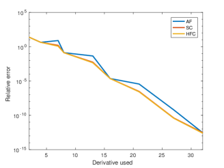
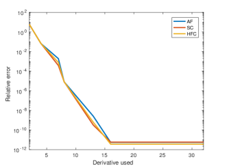
where (X0,Y0)subscript𝑋0subscript𝑌0(X_{0},Y_{0}) refer to a fixed position in the transversal plane. In figure 1, it is reported the behaviour of the error (33) for two different transversal positions, one closer to the quadrupole axis and another further away. The results refer to vector potentials in different gauges, computed considering a second order harmonic B2subscript𝐵2B_{2} coming from a realistic design of a quadrupole (see section 6). It can be noticed that the error in the different gauges coincides if ND𝑁𝐷ND is an even number, coherently with the fact that the magnetic fields are identical. It is unclear to which extent this approximation error, which is far from negligible at larger distances from the quadrupole axis, entails a limitation for the accuracy that tracking algorithms can achieve. Mimetic methods like those presented in Lipnikov et al. (2011) guarantee that a discrete equivalent of ××𝑨=0𝑨0{\nabla}\times{\nabla}\times{\boldsymbol{A}}=0 is exactly satisfied, so that they could represent a potentially interesting alternative to the techniques described in this section.
Refer to caption Refer to caption
Figure 1: Relative error in the Maxwell equation with respect to the number of generalized gradient derivatives used. Positions (X0,Y0)=(0,0.01)subscript𝑋0subscript𝑌000.01(X_{0},Y_{0})=(0,0.01) (left) and (X0,Y0)=(0,0.04)subscript𝑋0subscript𝑌000.04(X_{0},Y_{0})=(0,0.04) (right). Second order harmonic B2subscript𝐵2B_{2} of realistic case (sec. 6).

As a final remark we notice that, in the use of equation 20, particular attention has to be devoted to the computation of the input harmonics. If harmonics that do not go to zero sufficiently fast at the boundaries are employed, significant errors in the field description may result. For example, even if the harmonics vanish at the boundaries, the computed generalized gradients, and thus the vector potential, may not vanish as well, causing a discrepancy between the canonical and the mechanical momenta in a region where they should coincide. In our experience, these issues can be avoided by appropriate extension of the harmonics data by sufficiently large regions filled with zero values.

5 Numerical experiments with an analytic magnetic vector potential

In this section, equations (11) will be solved for the case of a simple vector potential, whose expression is given by a polynomial with just a few non zero coefficients. It is important to notice that this configuration is not completely realistic, since this vector potential does not exactly satisfy the Maxwell equation ××𝑨=0.𝑨0{\nabla}\times{\nabla}\times{\boldsymbol{A}}=0. As discussed in the previous section, this leads to spurious residual currents in the right hand side of this equation, which are however not accounted for in equations (11). In spite of this inconsistency, this benchmark is useful to assess the impact of the interpolation procedure mentioned in section 3, since the simple analytic expression can also be computed cheaply online and comparison between results obtained with and without interpolation can be carried out.

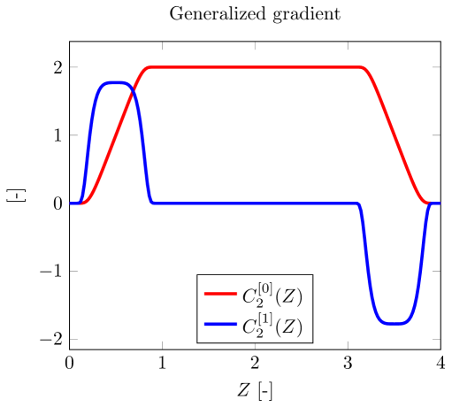
A set of scaled vector potentials in different gauges is built using equations (22), (23) and (28) and employing only the C2[0](Z)superscriptsubscript𝐶2delimited-[]0𝑍C_{2}^{[0]}(Z) function defined as follows. We first set

σ(x)={0x(,1]12[1+erf(tan(π2x))]x(1,1)1x[1,+)\sigma\left(x\right)=\left\{\begin{aligned} &0&&\qquad x\in\left(-\infty,-1\right]\\ &\dfrac{1}{2}\left[1+{\text{erf}\left({\tan\left(\dfrac{\pi}{2}\,x\right)}\right)}\right]&&\qquad x\in\left(-1,1\right)\\ &1&&\qquad x\in\left[1,+\infty\right)\end{aligned}\right. (34)

where erf denotes the error function, defined as

erf(x)=2π0xet2dt.erf𝑥2𝜋superscriptsubscript0𝑥superscript𝑒superscript𝑡2d𝑡{\text{erf}\left(x\right)}=\dfrac{2}{\sqrt{\pi}}\int_{0}^{x}e^{-t^{2}}\text{d}t\leavevmode\nobreak\ .

Using (34), the function C2[0](Z)superscriptsubscript𝐶2delimited-[]0𝑍C_{2}^{[0]}(Z) is then defined as

C2[0](Z)={α[σ(1+2ZL1)+σ(12ZZ2L2)]αZ(0,ZMAX)0otherwise.C_{2}^{[0]}(Z)=\left\{\begin{aligned} &\alpha\,\left[\sigma\left(-1+2\,\dfrac{Z}{L_{1}}\right)+\sigma\left(1-2\,\dfrac{Z-Z_{2}}{L_{2}}\right)\right]-\alpha&&\quad Z\in\left(0,\,Z_{MAX}\right)\\ &0&&\quad\text{otherwise.}\end{aligned}\right.

(35)

Here, the coefficient α𝛼\alpha is the plateau value of C2[0](Z)superscriptsubscript𝐶2delimited-[]0𝑍C_{2}^{[0]}(Z), ZMAXsubscript𝑍𝑀𝐴𝑋Z_{MAX} denotes the total field length, L1,L2subscript𝐿1subscript𝐿2L_{1},L_{2} are the widths of the regions in which the field is not constant and Z2subscript𝑍2Z_{2} denotes the location of the second of these regions, the first being located at Z=0𝑍0Z=0 (see figure 2).

Refer to caption
Figure 2: Analytic generalized gradient and its derivative.

In this work, the value α𝛼\alpha in (35) has been chosen equal to 61046superscript1046\cdot 10^{-4} with L1=L2=0.9subscript𝐿1subscript𝐿20.9L_{1}=L_{2}=0.9 and Z2=3.1.subscript𝑍23.1Z_{2}=3.1. The initial conditions for the transversal positions and momenta of the particle are set to 𝒘0=(0.02,0.04, 0, 0)subscript𝒘00.020.04 0 0{\boldsymbol{w}}_{0}=\left(0.02,\,-0.04,\,0,\,0\right) and δ0=0subscript𝛿00\delta_{0}=0. A reference solution is computed using the exact vector potential and the MATLAB ODE solver ode45 with a maximum ΔZref=ΔZdata/10Δsuperscript𝑍𝑟𝑒𝑓Δsuperscript𝑍𝑑𝑎𝑡𝑎10\Delta Z^{ref}=\Delta Z^{data}/10 and a relative error tolerance of 1013superscript101310^{-13}.

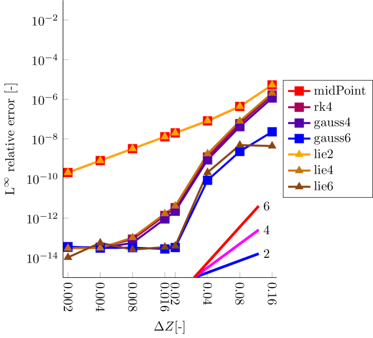
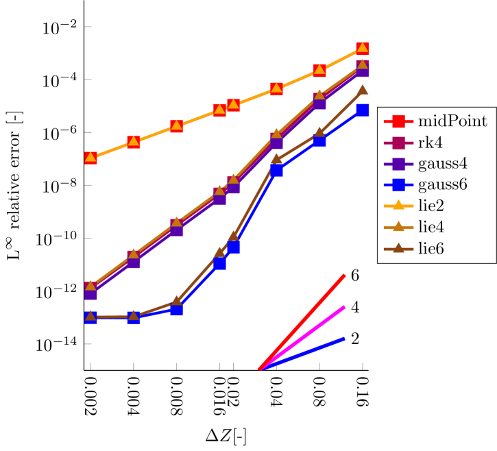
In figure 3, the errors obtained with the different ODE methods are presented, in the case in which no interpolation is used and the magnetic vector potential is computed exactly at each required location.
Refer to caption
Refer to caption
Figure 3: Test case with analytically defined vector potential. Convergence behaviour in the lsubscript𝑙l_{\infty} norm of different ODE methods for X𝑋X (left) and Pysubscript𝑃𝑦P_{y} (right) when exact vector potential values are employed at all intermediate steps. The straight lines in the bottom right corner denote theoretical slopes for different convergence orders.

The errors on the X,Y𝑋𝑌X,Y coordinates behave very similarly and the same is true for the corresponding moments, but the errors on transversal momenta are larger than those on positions. As long as the errors are above the tolerance chosen for the reference solution, both second and fourth order solvers behave in agreement with theoretical expectations, while sixth order solvers only seem to display the expected error decay for sufficiently small values of the interval ΔZ.Δ𝑍\Delta Z. Furthermore, very similar errors are obtained for second and fourth order methods for the largest ΔZΔ𝑍\Delta Z employed. We attribute these facts to the poor resolution of the larger gradient areas at the beginning and at the end of the idealized quadrupole. This effect can also be seen in the numerical results of section 6. It gives a clear indication that there is an upper limit to the value ΔZΔ𝑍\Delta Z that can be employed, independently of the accuracy of the solver employed.

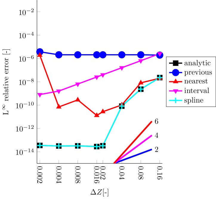
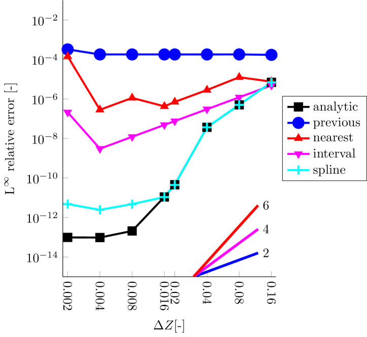
In order to study the impact of different interpolation techniques in the more realistic case in which the vector potential is only available as sampled data, the analytic vector potential obtained from (35) are sampled on a fine mesh with ΔZdata=0.002Δsuperscript𝑍𝑑𝑎𝑡𝑎0.002\Delta Z^{data}=0.002 over the interval [0,4]04[0,4]. For each given position along the Z𝑍Z axis where the vector potential is not available, we employ a) the value at the last previously available gridded location (previous), b) the value at the nearest gridded location available (nearest), c) the average of the nearest available potential values (interval) d) a cubic spline interpolation (spline). The results of this comparison are reported in figure 4. Only results obtained with the sixth-order Gauss method are displayed, since the highest order methods are those most affected by the accuracy of the field interpolation. It can be noticed that all interpolation methods limit the overall accuracy of the time integrator, to a larger or lesser extent. Ideally, an interpolator of the same order of the time integration method should be employed. On the other hand, spline interpolation seems to be sufficient to achieve errors comparable to those of the exact potential evaluation in most cases.
Refer to caption
Refer to caption
Figure 4: Test case with analytically defined vector potential. Convergence behaviour in the lsubscript𝑙l_{\infty} norm of different ODE methods for X𝑋X (left) and Pysubscript𝑃𝑦P_{y} (right) when reconstructed vector potential values are employed at all intermediate steps. The straight lines in the bottom right corner denote theoretical slopes for different convergence orders.

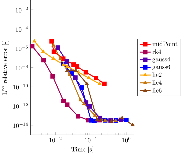
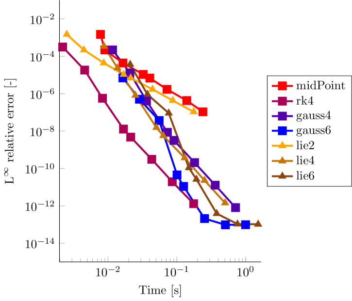
In order to compare the efficiencies of the methods employed, we report in figure 5 the behavior of the error as a function of the CPU time required by each method for a given resolution. Since the interpolation stage is done off-line, the CPU time required does not depend on the interpolation method employed. Among the ODE methods, the fourth-order explicit Runge-Kutta method gives the best results, followed by the sixth-order Gauss method and the fourth-order Lie method. Among the symplectic methods, the fastest method is the second-order Lie one, but it has a relatively low accuracy.
Refer to caption
Refer to caption
Figure 5: Analytic case, no interpolation. Efficiency comparison between ODE methods for X𝑋X (left) and Pysubscript𝑃𝑦P_{y} (right).

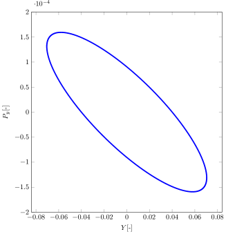
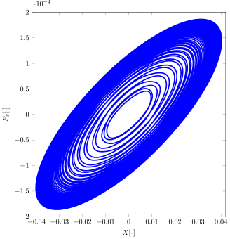
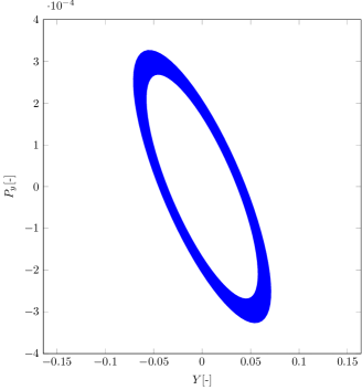
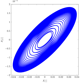
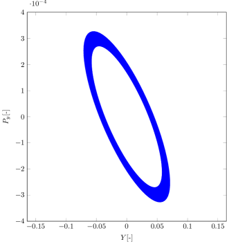
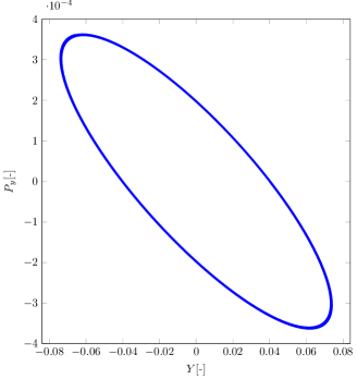
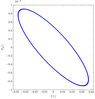
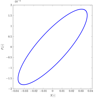
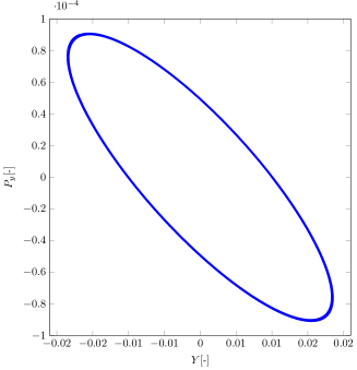
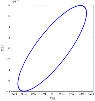
As mentioned in the introduction, the beam stability assessment requires long-term simulations. In order to verify the solution quality in this framework, the phase-space orbits of a particle which travels through a sequence of focusing-defocusing quadrupole couples are measured. This test is carried out considering a sequence of 300030003000 consecutive quadrupole couples and an integration step of ΔZ=0.08Δ𝑍0.08\Delta Z=0.08. All the numerical methods produced stable orbits in this test. As an example, in figure 6 the results for the fourth-order Lie method are reported. Remarkably, the non-symplectic fourth-order Runge-Kutta method gives results entirely analogous to those of the other (symplectic) methods considered, see figure 7.
Refer to caption Refer to caption
Figure 6: Analytic case, cubic spline interpolation. Phase-space trajectories in the (X,Px)𝑋subscript𝑃𝑥\left(X,P_{x}\right) (left) and (Y,Py)𝑌subscript𝑃𝑦\left(Y,P_{y}\right) (right) planes, X0=0.02subscript𝑋00.02X_{0}=-0.02, Y0=0.04subscript𝑌00.04Y_{0}=0.04. Fourth-order Lie method.
Refer to caption Refer to caption
Figure 7: Analytic case, cubic spline interpolation. Phase-space trajectories in the (X,Px)𝑋subscript𝑃𝑥\left(X,P_{x}\right) (left) and (Y,Py)𝑌subscript𝑃𝑦\left(Y,P_{y}\right) (right) planes, X0=0.02subscript𝑋00.02X_{0}=-0.02, Y0=0.04subscript𝑌00.04Y_{0}=0.04. Fourth-order explicit Runge-Kutta method.

6 Numerical experiments with a realistic vector potential

In this section, equations (11) will be solved for the case of a magnetic vector potential that corresponds to the design of a realistic quadrupole. The harmonics m=2, 6, 10, 14𝑚261014m=2,\,6,\,10,\,14, at a radius of analysis of 0.050.050.05 and sampled at ΔZdata=0.02Δsuperscript𝑍𝑑𝑎𝑡𝑎0.02\Delta Z^{data}=0.02 (figure 8) are provided by numerical simulations performed by the FEM/BEM software ROXIE rox (2018), used at CERN to design the accelerator magnets. The presence of connectors on one side of the quadrupole causes asymmetries in the harmonics along the Z𝑍Z axis and the presence of skew harmonics.
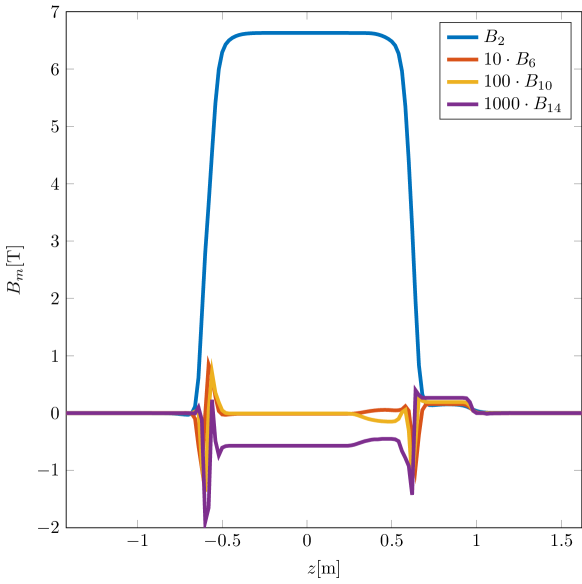
Refer to caption
Figure 8: Realistic case. Normal harmonics sampled at Δzdata=0.02mΔsuperscript𝑧𝑑𝑎𝑡𝑎0.02m\Delta z^{data}=0.02\,\text{m}.

The generalized gradients are computed using up to 161616 derivatives. We will consider the case of a particle quite far from the quadrupole axis: indeed, the initial conditions for the transversal positions and momenta are set to 𝒘0=(0.02,0.04, 0, 0)subscript𝒘00.020.04 0 0{\boldsymbol{w}}_{0}=\left(0.02,\,-0.04,\,0,\,0\right) and δ0=0subscript𝛿00\delta_{0}=0. Using the horizontal-free Coulomb gauge, we obtain a gain in efficiency quite in agreement with the estimates given in section 4, see tables 4 and 5.

Time [s] Ratio [-]
ΔZΔ𝑍\Delta Z [-] AF HFC HFC/AF
0.020.020.02 0.05990.05990.0599 0.03410.03410.0341 0.57040.57040.5704
0.040.040.04 0.02710.02710.0271 0.01660.01660.0166 0.61310.61310.6131
0.080.080.08 0.01330.01330.0133 0.00840.00840.0084 0.63480.63480.6348
0.160.160.16 0.00710.00710.0071 0.00430.00430.0043 0.60410.60410.6041
Average 0.6060.606\mathbf{0.606}
Table 4: Realistic case. CPU time and speed-up obtained using different vector potential gauges and the fourth-order explicit Runge-Kutta method.
Time [s] Ratio [-]
ΔZΔ𝑍\Delta Z [-] AF HFC HFC/AF
0.020.020.02 0.09660.09660.0966 0.05480.05480.0548 0.56800.56800.5680
0.040.040.04 0.04740.04740.0474 0.02560.02560.0256 0.54010.54010.5401
0.080.080.08 0.02410.02410.0241 0.01320.01320.0132 0.54770.54770.5477
0.160.160.16 0.01180.01180.0118 0.00680.00680.0068 0.57260.57260.5726
Average 0.5570.557\mathbf{0.557}
Table 5: Realistic case. CPU time and speed-up obtained using different vector potential gauges and the fourth-order Lie method.

In the following, only the results with the horizontal-free Coulomb gauge and using cubic spline interpolation of gridded data are reported.

The error comparisons are shown in figure 9. In order to measure the methods’ accuracy, the absolute error on the positions and the momenta at the quadrupole exit are used, because these values are useful to to understand if the non-linear effects, mentioned in the introduction, can be described correctly.
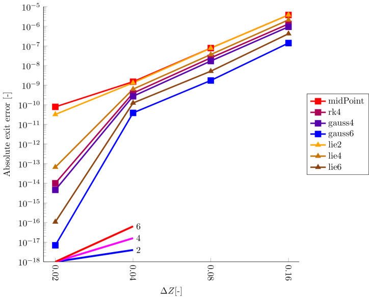
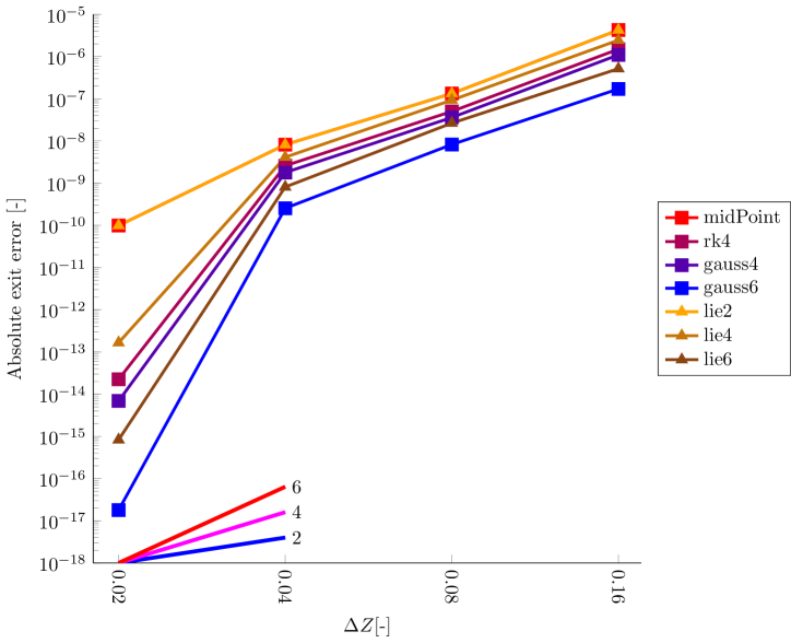
Refer to caption
Refer to caption
Figure 9: Realistic case, cubic spline interpolation. Error comparison between ODE methods for X𝑋X (left) and Pysubscript𝑃𝑦P_{y} (right). The straight lines in the bottom right corner correspond to the theoretical slopes of the error curves for different convergence orders.

The trend is similar to those seen in the previous sections, but with a general worsening in accuracy. Longer time integration steps prevent the correct description of the field and consequently the achievement of the theoretical convergence orders for the numerical methods. The final error drops in the high-order methods can be due to the fact that the reference solution has been computed using the same starting vector potential data and only a finer mesh of interpolated values. In order to compare the efficiencies of the methods employed, we plot in figure 10 the behaviour of the error as a function of the CPU time required by each method for a given resolution.
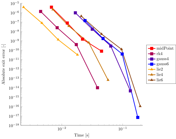
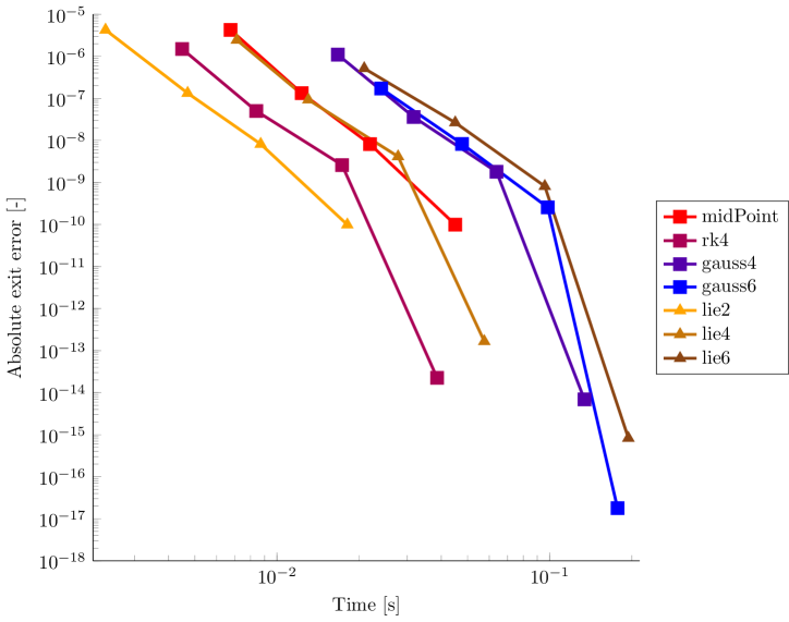
Refer to caption
Refer to caption
Figure 10: Realistic case, cubic spline interpolation. Efficiency comparison between ODE methods for X𝑋X (left) and Pysubscript𝑃𝑦P_{y} (right).

In this case, the large ΔZdataΔsuperscript𝑍𝑑𝑎𝑡𝑎\Delta Z^{data} of the input data limits the possibility of achieving high accuracies, therefore there is no clear advantage in the use of high order methods and the second-order Lie method is the most efficient.

Finally, we check the beam stability looking at the phase-space orbits of a particle which travels through a sequence of focusing-defocusing quadrupole couples. This test is carried out considering a sequence of 240002400024000 consecutive quadrupole couples and an integration step of ΔZ=0.04Δ𝑍0.04\Delta Z=0.04. In this case it is possible to notice (see figures 11 and 12) that the trend in the (X,Px)𝑋subscript𝑃𝑥\left(X,P_{x}\right) phase space appears unstable.

Refer to caption Refer to caption
Figure 11: Realistic case, cubic spline interpolation. Phase-space trajectories in the (X,Px)𝑋subscript𝑃𝑥\left(X,P_{x}\right) (left) and (Y,Py)𝑌subscript𝑃𝑦\left(Y,P_{y}\right) (right) planes, X0=0.02subscript𝑋00.02X_{0}=0.02, Y0=0.04subscript𝑌00.04Y_{0}=-0.04. Fourth-order Lie method.
Refer to caption Refer to caption
Figure 12: Realistic case, cubic spline interpolation. Phase-space trajectories in the (X,Px)𝑋subscript𝑃𝑥\left(X,P_{x}\right) (left) and (Y,Py)𝑌subscript𝑃𝑦\left(Y,P_{y}\right) (right) planes, X0=0.02subscript𝑋00.02X_{0}=0.02, Y0=0.04subscript𝑌00.04Y_{0}=-0.04. Fourth-order explicit Runge-Kutta method.

The instability is probably due to the high degree of the vector potential polynomial, obtained using various harmonics and many generalized gradient derivatives. In fact, using only the second order harmonic and two generalized gradient derivatives (figure 13), or considering a motion closer to the center (figure 14), it is possible to obtain stable orbits similar to the ones obtained in the analytical case presented in section 5.
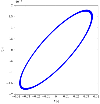
Refer to caption Refer to caption
Figure 13: Realistic case II, second order harmonic, two generalized gradient derivatives, cubic spline interpolation. Phase-space trajectories in the (X,Px)𝑋subscript𝑃𝑥\left(X,P_{x}\right) (left) and (Y,Py)𝑌subscript𝑃𝑦\left(Y,P_{y}\right) (right) planes, X0=0.02subscript𝑋00.02X_{0}=-0.02, Y0=0.04subscript𝑌00.04Y_{0}=0.04. Fourth-order Lie method.
Refer to caption Refer to caption
Figure 14: Realistic case II, cubic spline interpolation. Phase-space trajectories in the (X,Px)𝑋subscript𝑃𝑥\left(X,P_{x}\right) (left) and (Y,Py)𝑌subscript𝑃𝑦\left(Y,P_{y}\right) (right) planes, X0=0.02subscript𝑋00.02X_{0}=-0.02, Y0=0.01subscript𝑌00.01Y_{0}=0.01. Fourth-order Lie method.

It is especially noteworthy that, in spite of its lack of symplectic properties, the classical fourth order RK method does not appear to behave differently with respect to the symplectic ones (figures 15 and 16).

Refer to caption Refer to caption
Figure 15: Realistic case II, second order harmonic, two generalized gradient derivatives, cubic spline interpolation. Phase-space trajectories in the (X,Px)𝑋subscript𝑃𝑥\left(X,P_{x}\right) (left) and (Y,Py)𝑌subscript𝑃𝑦\left(Y,P_{y}\right) (right) planes, X0=0.02subscript𝑋00.02X_{0}=-0.02, Y0=0.04subscript𝑌00.04Y_{0}=0.04. Fourth-order explicit Runge-Kutta method.
Refer to caption Refer to caption
Figure 16: Realistic case II, cubic spline interpolation. Phase-space trajectories in the (X,Px)𝑋subscript𝑃𝑥\left(X,P_{x}\right) (left) and (Y,Py)𝑌subscript𝑃𝑦\left(Y,P_{y}\right) (right) planes, X0=0.02subscript𝑋00.02X_{0}=-0.02, Y0=0.01subscript𝑌00.01Y_{0}=0.01. Fourth-order explicit Runge-Kutta method.

Finally, we check the energy conservation for a particle which travels through 800080008000 focusing-defocusing quadrupole pairs using an integration step ΔZ=0.08Δ𝑍0.08\Delta Z=0.08. Results are shown in figure 17.

Refer to caption
Refer to caption
Figure 17: Realistic case II, cubic spline interpolation. Trend of the 𝒦Xsubscript𝒦𝑋\mathcal{K}_{X} (left) energy component along 800080008000 focusing-defocusing quadrupole couples for different ODE methods and deviation of 𝒦Xsubscript𝒦𝑋\mathcal{K}_{X} associated to the different methods with respect to the sixth-order Gauss method (right).

In this realistic case the magnetic vector potential has a more complex shape and the differences in the 𝒦Xsubscript𝒦𝑋\mathcal{K}_{X} trend among the numerical methods appear sooner. Nevertheless, the 𝒦Xsubscript𝒦𝑋\mathcal{K}_{X} oscillations appear to be stable and no significant differences between symplectic and non symplectic methods concerning the energy conservation are observed.

7 Conclusions and future developments

We have discussed and analyzed several issues that arise in the numerical approximation of charged particles trajectories in magnetic quadrupoles. We have shown that a specific gauge transformation that allows to reduce by approximately 50% the computational cost of each vector potential evaluation, thus significantly enhancing the efficiency of any numerical approximation method employed for the particle trajectory simulation.

The impact of the interpolation technique employed to compute magnetic vector potential values at arbitrary locations from gridded data has also been assessed, highlighting potential limitations in accuracy induced by insufficiently accurate interpolation methods, if high order time integration techniques are to be applied. However, cubic spline interpolation was found to be sufficient for preserving the accuracy of all the methods considered in this work over a wide range of values for the integration step.

We have then compared several high order integration techniques, which allow to maintain high accuracy even with relatively large integration step values, in order to assess their accuracy and efficiency for long-term simulations. Explicit high order Lie methods have been considered, along with implicit high order symplectic integrators and a more conventional, non symplectic explicit Runge-Kutta methods.

In the case of realistic vector potentials, the errors induced by the vector potential representation and interpolation become significant and reduce the highest possible accuracy that can be attained. Furthermore, since in realistic cases the magnetic vector potential evaluation costlier, numerical methods which require less evaluations, such as the second-order Lie method, appear to be more competitive in terms of efficiency. On the other hand, if these errors could be reduced by different approaches for the vector field representation, higher order methods could be advantageous if a more precise approximation is required. The speed gain obtained by the horizontal-free Coulomb gauge would also allow to use more expensive methods. In particular, the explicit fourth-order Runge-Kutta appears to be the most efficient method and the fourth-order Lie the most efficient among symplectic methods.

All the computations carried out in this work employed vector potential values sampled on a uniform grid along the longitudinal axis of the quadrupole. In order to increase the efficiency of the methods employed, using vector potentials sampled over a non-uniform grid appears to be a straightforward and necessary improvement. In such way, it could be possible to use a smaller step in the fringe field regions, where the vector potential has more complex shape, and a larger step where the field is uniform and has simpler structure.

A particularly interesting aspect of the results obtained was the fact that non symplectic methods appeared to be competitive with symplectic ones, even on relatively long integrations. An even more extreme example of this behaviour was seen in the simulation of a particle crossing 160000016000001600000 quadrupole couples of realistic design (323232 quadrupoles in 100000100000100000 revolutions). An integration step ΔZ=0.16Δ𝑍0.16\Delta Z=0.16 was employed. As shown in figure 18, even in this extremely long simulation the behaviour of a symplectic Lie method and of a non symplectic Runge Kutta method was entirely analogous in terms of energy conservation, in contrast to the theoretical expectations.
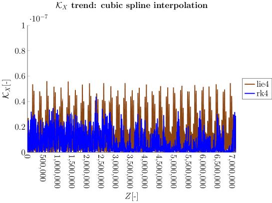
Refer to caption
Figure 18: Energy conservation of a particle through 160000016000001600000 focusing-defocusing quadrupole couples using the fourth-order explicit Runge-Kutta and the fourth-order Lie method.

It would be interesting to understand whether more realistic test cases could actually highlight negative effects induced by non-symplectic methods and whether more detailed monitoring of the particle motion could be employed for this purpose. For example, in this work only the energy associated to the transverse variable was used to measure the good behaviour in long-term simulations. Other conserved quantities could also be used to compare the performance of the different methods.

Acknowledgements

This paper contains an extension of results initially presented in the Master Thesis of A.S., who was partially supported by CEA Saclay, where part of this work was carried out.

References

  • rox [2018] ROXIE - software for electromagnetic simulation and optimization of accelerator magnets. https://espace.cern.ch/roxie/default.aspx, 2018.
  • Carey [1988] D. C. Carey. The optics of charged particle beams. Applied Optics, 27:1002, 1988.
  • Corno et al. [2016] J. Corno, C. de Falco, H. De Gersem, and S. Schöps. Isogeometric simulation of Lorentz detuning in superconducting accelerator cavities. Computer Physics Communications, 201:1–7, 2016.
  • Dalena and Pugnat [2015] B. Dalena and T. Pugnat. Calcul d’une carte de transport réaliste pour particules chargées. Technical report, Centre Energie Atomique, 2015.
  • Dalena et al. [2014] B. Dalena, O. Gabouev, M. Giovannozzi, R. De Maria, R.B. Appleby, A. Chancé, J. Payet, and D.R. Brett. Fringe fields modeling for the high luminosity LHC large aperture quadrupoles. Technical Report CERN-ACC-2014-0175, CERN, 2014.
  • Dragt [1997] A.J. Dragt. Lie methods for nonlinear dynamics with applications to accelerator physics. University of Maryland, Center for Theoretical Physics, Department of Physics, 1997. URL http://www.physics.umd.edu/dsat/.
  • Forest [1998] E. Forest. Beam Dynamics. CRC Press, 1998.
  • Hairer et al. [2006] E. Hairer, C. Lubich, and G. Wanner. Geometric numerical integration: structure-preserving algorithms for ordinary differential equations. Springer Science & Business Media, 2006.
  • Kotkin and Serbo [2013] G.L. Kotkin and V. G. Serbo. Collection of Problems in Classical Mechanics: International Series of Monographs in Natural Philosophy, volume 31. Elsevier, 2013.
  • Lipnikov et al. [2011] K. Lipnikov, G. Manzini, F. Brezzi, and A. Buffa. The mimetic finite difference method for the 3D magnetostatic field problems on polyhedral meshes. Journal of Computational Physics, 230(2):305–328, 2011.
  • Panofsky and Phillips [1962] W.K. H. Panofsky and M. Phillips. Classical electricity and magnetism. Addison Wesley, 1962.
  • Rossi [2011] L. Rossi. LHC upgrade plans: Options and strategy. In Second International Particle Accelerator Conference, San Sebastian, 2011.
  • Venturini and Dragt [1999] M. Venturini and A.J. Dragt. Accurate computation of transfer maps from magnetic field data. Nuclear Instruments and Methods in Physics Research Section A: Accelerators, Spectrometers, Detectors and Associated Equipment, 427(1):387–392, 1999.
  • Wu et al. [2003] Y.K. Wu, E. Forest, and D.S. Robin. Explicit symplectic integrator for slimit-from𝑠s-dependent static magnetic field. Physical Review E, 68(4):046502, 2003.
  • Yoshida [1990] H. Yoshida. Construction of higher order symplectic integrators. Physics Letters A, 150(5):262–268, 1990.