A novel incentive-based demand response model for Cournot competition in electricity markets

Abstract

This paper presents an analysis of competition between generators when incentive-based demand response is employed in an electricity market. Thermal and hydropower generation are considered in the model. A smooth inverse demand function is designed using a sigmoid and two linear functions for modeling the consumer preferences under incentive-based demand response program. Generators compete to sell energy bilaterally to consumers and system operator provides transmission and arbitrage services. The profit of each agent is posed as an optimization problem, then the competition result is found by solving simultaneously Karush–Kuhn–Tucker conditions for all generators. A Nash-Cournot equilibrium is found when the system operates normally and at peak demand times when DR is required. Under this model, results show that DR diminishes the energy consumption at peak periods, shifts the power requirement to off-peak times and improves the net consumer surplus due to incentives received for participating in DR program. However, the generators decrease their profit due to the reduction of traded energy and market prices.

1 Introduction

Demand Response (DR) is a program to motivate changes in electricity usage by customers in response to changes in the price signal. DR is implemented by system operator (SO) to match the load with power generation in a smart grid. Advanced metering at distribution side is required to implement a DR program (Aketi and Sen, 2014). The main application is to decrease the load at peak times in order to guarantee power availability and security on electrical grid (Zhu et al., 2013; Bloustein, 2005; Su and Kirschen, 2009). The aim is to control noncritical loads at residential, commercial and industrial levels for balancing supply and demand. Broadly speaking, there are two ways to active DR: direct control (e.g. load shedding or set-point based solutions) (Diaz et al., 2017) and indirect methods (such as price-based programs) (Vuelvas and Ruiz, 2017).

There are some DR programs implemented as part of strategies to reduce peak power. In (Vardakas et al., 2015; Deng et al., 2015; Siano, 2014; Albadi and El-Saadany, 2008; Madaeni and Sioshansi, 2013), some complete summaries regarding mathematical models, pricing methods, optimization formulation and future extensions are described. An interesting program to induce DR is via incentive payment (an indirect control) by using a technique called Peak Time Rebate (PTR) (Vuelvas and Ruiz, 2017, 2015; Mohajeryami et al., 2016a; Severin Borenstein, 2014), where customers receive electricity bill rebates by not consuming (relative to a previously established, household-specific baseline) during peak periods. In PTR, the baseline is a vital concept since the payment depends on the calculation of estimated consumption, namely, a counterfactual model must be developed. In (Mohajeryami et al., 2016a), some methods are explained to estimate the customer baseline. A randomized controlled trial method is developed in order to establish customer baseline load, applied to aggregated forms of the consumption load in (Mohajeryami et al., 2016b). The critical facts on the selection of customer baseline is shown in (Chao, 2011), authors design a suitable baseline focusing on administrative and contractual approaches in order to get an efficient DR. Furthermore, in (Faria et al., 2013; Wijaya et al., 2014; Antunes et al., 2013), the performance of DR baseline estimation models is studied and new methods are regarded as establishing the reasonable compensation for the consumer.

The co-existence of a variety of generation technologies is an interesting problem from a gaming point of view and even more with the integration of DR into the electricity market. In (Genc and Thille, 2008), the competition between hydro and thermal electricity generators under uncertainty over demand and water flows is presented. The authors in (Garcia et al., 2005) analyze the price-formation in an oligopoly model where hydroelectric generators are involved in dynamic Bertrand competition. Furthermore, in (Villar and Rudnick, 2003), a model to understand a hydrothermal electric power market is built based on simple bids to the SO. Moreover, in (Zhu et al., 2013), by means of Stackelberg game is illustrated what is the value that DR management can bring to generation companies and consumers in a smart grid. In (Su and Kirschen, 2009), a method is devised for quantifying the effect of the demand response for the market as a whole.

The agents involved in an electricity market in competition with DR are shown in Fig. 1. In this paper, SO is responsible for arbitrage services in order to establish a proper environment for competition and gaming. The generators have different technologies, costs, revenues, and each firm seeks to maximize its profit (the difference between producers’ revenue and costs). Furthermore, the aggregators carry out the request to users of reducing energy consumption, namely, DR process. The main goal is to estimate the equilibrium price under gaming environment. This competition is less than perfect, some firms are able to influence the market price through their actions. Such optimization problems set up which is called in game theory a non-cooperative game (Vega Redondo, 2003; Gabriel et al., 2013; Tirole, 1988; Osborne, 1995; Varian, 1992). The solution of such a game is called a Nash equilibrium and represents a market equilibrium under imperfect competition.

In this paper, a game among generators with different technologies in an electricity market is analyzed if DR is required when the demand side exceed a defined threshold a priori by SO in order to guarantee some objectives of a smart grid. This threshold is determined from all customer baseline load and desired energy reduction during peak times. Then, a novel demand curve is proposed in order to understand the effect of electricity market behavior when an incentive-based DR program, like PTR, is held to diminish the energy consumption at the peak periods.

Figure 1: Gaming in the electricity market. Where $n_{g}$ and $n_{d}$ are the total number of generators and aggregators in the electricity market, respectively.

The contributions of this paper are summarized as follows:

• A novel incentive-based DR model is proposed. Demand function is formulated by using a sigmoid function between two linear polynomials to depict the energy threshold when DR is required. This formulation is a continuous function with finite marginal value in the demand curve. In particular, it is an alternative modeling of DR to (Su and Kirschen, 2009), where, the demand curve has two parts: perfect inelastic behavior and price responsive consumers. The inconvenience of (Su and Kirschen, 2009) is that demand does no have perfect inelastic role since the consumers have a limited willingness to pay.

• A Nash-Cournot equilibrium is formulated as a complementary problem in the presence of DR (Gabriel et al., 2013). The generators compete without a centralized program. Cournot gaming is compared when an electricity market operates normally and when an incentive-based DR is active during peak times.

The rest of this paper is organized as follows. Section II introduces the agent models in an electricity market. Section III, the problem formulation as Cournot Competition in the presence of DR is developed. Numerical results are described in Section IV. Discussion is presented in Section V. Finally, conclusions are drawn in Section VI.

2 Agent models

In this section, a novel demand model is proposed for studying an incentive-based DR program within an electricity market. This formulation illustrates the wholesale market behavior during a day. In addition, generator models are posed under Cournot Competition.

2.1 Demand response model

The most important decision unit of microeconomic theory is the demand (Varian, 1992; Mas-Colell et al., 1995). In this section, a new approach for modeling the demand is posed when consumers participate in an incentive-based DR program. Let $T=\left\{1,2,...,n_{t}\right\}$ be the set of periods to take into account in the horizon time, where $n_{t}$ is last hour, that is, $n_{t}=24$. An aggregated demand is considered for this DR rebate model. The decision-maker’s preferences are specified by giving smooth utility function $G(q_{t})$, where $q_{t}$ is the energy consumption at time $t$. $G(q_{t})$ depicts the level of satisfaction obtained by the demand as a function of the total power consumption.The utility function satisfies the following properties as proposed in (Chen et al., 2012; Samadi et al., 2012; Fahrioglu and Alvarado, 2000; Vega Redondo, 2003; Osborne, 1995):

Property 1: $G(q_{t})$ is assumed as a concave function with respect to $q_{t}$. This implies that the marginal benefit of users is a nonincreasing function.

$$\frac{d^{2}G(q_{t})}{dq_{t}^{2}}\leq 0\quad\forall t\in T$$

Property 2: The marginal benefit is nonnegative.

$$\frac{dG\left(q_{t}\right)}{dq_{t}}\geq 0\quad\forall t\in T$$

Property 3: $G(q_{t})$ is zero when the consumption level is zero.

$$G\left(0\right)=0\quad\forall t\in T$$

The market price is $p_{t}^{*}$ at the time $t$. The superscript star indicates the equilibrium price. For each generator, the cost function is assumed increasing with respect to the total energy production capacity. In addition, the cost function is strictly convex. Then, other definitions are considered as follows.

Definition 1

The demand energy total cost is $\pi(q_{t})=p_{t}^{*}q_{t}$.

Definition 2

$G(q_{t})$ is approximated by a second order polynomial around $\overline{q}_{t},\quad\forall t\in T$. In general, a quadratic function is considered.

$$G\left(q_{t}\right)=-\frac{\gamma_{t}}{2}\left(q_{t}-\overline{q}_{t}\right)^{2}+p_{t}^{*}\left(q_{t}-\overline{q}_{t}\right)+k\quad\forall t\in T$$

being $k=\overline{q}_{t}\left(\frac{\gamma_{t}}{2}\overline{q}_{t}+p_{t}^{*}\right)$ a constant value, obtained by Property 3.

Definition 3

The payoff function is defined as $U_{t}\left(q_{t}\right)=G(q_{t})-\pi(q_{t})$, which indicates the user benefit of consuming $q_{t}$ energy during the interval $t$.

Basically, incentive-based DR programs request customers for curtailing demand in response to a price signal or economic incentive. Typically the invitation to reduce demand is made for a specific time period or peak event. There are some concepts in order to define DR rebate program:

Definition 4

Baseline ($\beta_{t}$): the amount of energy the user would have consumed in the absence of a request to reduce (counterfactual model) (Deng et al., 2015). This quantity can not be measured, then this is estimated from the previous consumption of the agent. In this work, the aggregated baseline corresponds to the sum of all customer baseline loads in order to propose a DR threshold required in the electricity market.

$q_{t}$ is the actual use, namely, the amount of energy that aggregated demand actually consumes during the event period.

Definition 5

Load Reduction ($\triangle_{t}\left(\beta_{t},q_{t}\right)$): the difference between the baseline and the actual use.

$$\beta_{t}-q_{t}=\triangle_{t}$$

In incentive-based DR programs, the rebate is only received if there is an energy reduction. Otherwise, the user does not get any incentive or penalty. Mathematically,

Definition 6

Let $p_{2}$ be the rebate price received by the demand due to energy reduction in peak periods. The DR incentive $\pi_{2}$ is given by,

$$\pi_{2}\left(q_{t};p_{2t},\beta_{t}\right)=\left\{\begin{array}[]{cc}p_{2t}\triangle_{t}=p_{2t}(\beta_{t}-q_{t})&q_{t}<\beta_{t}\\ 0&q_{t}\geq\beta_{t}\end{array}\right.\quad\forall t\in T$$

Next, the demand payoff function with DR rebate program is written as:

$$\hat{U_{t}}\left(q_{t};p_{2t},\beta_{t}\right)=G(q_{t})-\pi(q_{t})+\pi_{2}(q_{t};p_{2t},\beta_{t})\quad\forall t\in T$$ (1)

In this paper, the inverse demand function is formulated to develop the Cournot’s model of oligopoly. The inverse demand function is given by $p_{t}\left(q_{t}\right)=\frac{dU_{t}\left(q_{t}\right)}{dq_{t}}$. Where $p_{t}\left(q_{t}\right)$ is the price function at the time $t$.

Accordingly, the inverse demand function without DR is obtained from definition 3. Next, the linear inverse demand function is derived as follows.

$$p_{t}\left(q_{t}\right)=-\gamma_{t}q_{t}+\gamma_{t}\overline{q_{t}}\quad\forall t\in T$$ (2)

Whether the demand payoff function with DR is considered when $q_{t}<\beta_{t}$, then the inverse demand function is given by,

$$\widetilde{p_{t}}\left(q_{t}\right)=-\gamma_{t}q_{t}+\left(\gamma_{t}\overline{q_{t}}-p_{2t}\right)\quad\forall t\in T$$ (3)

In order to model the electricity market with DR during peak hours, a sigmoid function between both inverse demand functions (Eq. (2) and Eq. (3)) is proposed. Fig. 2 (a) depicts a novel demand function that models incentive-based DR at market level. The novel inverse demand function is presented as follows.

$$\hat{p_{t}}\left(q_{t}\right)=-\gamma_{t}q_{t}+\left(\gamma_{t}\overline{q_{t}}-\frac{p_{2t}}{1+e^{\alpha(-q_{t}+\xi)}}\right)\quad\forall t\in T$$ (4)

Figure 2: Inverse demand function.

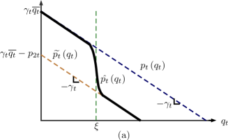
where $\alpha$ is a constant value which represents the smoothness of the sigmoid function that joins the two straight lines and $\xi$ is the threshold level to perform the DR process.
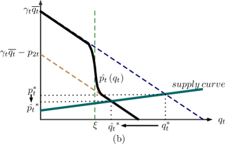
Notice that this demand model represents a preference alteration of consumers. Fig 2 (b) shows the case when the supply curve is intersected by demand curve for $q_{t}>\beta_{t}$. The equilibrium price $\hat{p_{t}}^{*}$ is less than the energy price given by the inverse demand function $p_{t}\left(q_{t}\right)$. In addition, the energy consumption decreases to $\hat{q_{t}}^{*}$ owing to the incentive price $\pi_{2}$, which is requested by setting the threshold $\xi$. The incentive is paid to consumers when the DR program is required. Besides, SO determines the threshold $\xi$ according to the available energy (water reservoirs, fuels, etc.), the estimated baseline $\beta_{t}$ and the energy consumption patterns. Then aggregators encourage customers for carrying out the energy reduction.

In (Su and Kirschen, 2009), the demand model has two parts: consumers that have perfect inelastic behavior, they are represented by an infinite marginal value; and users that participate in a DR program, they can place bid price with a finite marginal value in the demand curve. However, the drawback of the proposal (Su and Kirschen, 2009) is that demand does not have perfect inelastic behavior because the consumers have a limit willingness for energy payment. In this paper, demand always has a finite marginal value, hence, this model is an alternative to represent the DR behavior in an electricity market.

2.2 Supply model

The relationship between total energy from all generators and price lead to make the supply curve. In this work, producers try to anticipate the results of their actions on the price, then the market experiences imperfect competition. SO has arbitrage services, commands DR threshold, and manages the transmission assets as its functions into the electricity market. Therefore, each generator seeks independently to maximize its own economic benefits. The profit is given by its revenue from sold energy minus the cost of generating it. Two kinds of power suppliers are considered: thermal generators are represented with quadratic costs and hydropower are formulated with fixed costs (Genc and Thille, 2008).

2.2.1 Thermal generation modeling

The thermal cost is given by an increasing quadratic function. Let $r_{ta}$ be the power generated by producer $a\in A$ at the period $t$, where $A$ is the set of thermal generators. Thus, the costs have the following form: $c1_{a}r_{ta}+\frac{c2_{a}}{2}r_{ta}^{2}+c3_{a}$, being $c1_{a}$, $c2_{a}$ and $c3_{a}$ constant values that depict private information. These quadratic costs are stated because thermal power has an expensive economic behavior (Genc and Thille, 2008). In this sense, each generator uses its knowledge of the inverse demand function ($p_{t}\left(q_{t}\right)$ or $\hat{p_{t}}\left(q_{t}\right)$) to anticipate its own effect on the market price in order to maximize its profit. Then, the optimization problem for thermal generator is posed as follows.

$$\begin{array}[]{c}\max\;\sum_{t\in T}\left[p_{t}\left(q_{t}\right)r_{ta}-\left(c1_{a}r_{ta}+\frac{c2_{a}}{2}r_{ta}^{2}+c3_{a}\right)\right]\\ \begin{array}[]{cc}\mathrm{s.t.}&r_{ta}\leq r_{a}^{+}\,:\,\mu_{ta}^{T}\quad\forall t\in T\\ &r_{ta}\geq 0\quad\forall t\in T\end{array}\end{array}$$ (5)

where $r_{a}^{+}$ is the maximum value of the energy that each thermal power can generate in each period. $\mu_{ta}^{T}$ is dual variable for the first constraint. This model does not consider ramp constraint, minimum uptime and downtime, among other constraints.

2.2.2 Hydropower modeling

Hydropower is included in competition into the electricity market. The hydro generator has a production function $H_{tb}(w_{tb})$ which represents the conversion of water release to energy, where $w_{tb}$ is the water release of hydro reservoir for each generator $b\in B$. For this kind of producer, a fixed cost $c4_{b}$ is formulated. Hence, the optimization problem is to maximize the profits by each hydropower.

$$\begin{array}[]{c}\max\;\sum_{t\in T}\left[p_{t}\left(q_{t}\right)H_{tb}(w_{tb})-c4_{b}\right]\\ \begin{array}[]{cc}\mathrm{s.t.\>}&w_{tb}\leq w_{tb}^{+}\,:\,\mu_{tb}^{H}\>\forall t\in T\\ &w_{tb}\geq 0\>\forall t\in T\end{array}\end{array}$$ (6)

where $w_{tb}^{+}$ is the maximum value of the water release at the time $t$ for the generator $b$. $\mu_{tb}^{H}$ is dual variable for the first constraint.

3 Incentive-based demand response in Cournot competition

A Cournot competition is developed for studying the proposed DR model that is described in section 2. This model assumes that generators cannot collude or form a cartel, and they seek to maximize their own profit based on demand model. This section describes the game between market participants in order to settle the energy price by solving simultaneously the optimization problems (5) and (6), as presented in (Gabriel et al., 2013). Now, the definition of Nash equilibrium is stated as follows.

Definition 7

Considering the game $G=\left\langle I,\left\{S_{i}\right\}_{i=1,2,..n_{i}.},\left\{\psi_{i}\right\}_{i=1,2,...,n_{i}.}\right\rangle$, where $I$ is the players set, $S_{i}$ is the strategies set of each player and $\psi_{i}\,:\,\prod_{i\in I}S_{i}\rightarrow\mathbb{R}$ is the utility function of each generator. $\left(s_{1}^{*},...s_{i}^{*}\right)$ is a Nash equilibrium whether $\forall i\in I$ player is true that: $\psi_{i}\left(s_{i}^{*},s_{-i}^{*}\right)\geq\psi_{i}\left(s_{i},s_{-i}^{*}\right)$, $\forall s_{i}\in S_{i}$, being $s_{-i}$ all strategies except the player $i$ (Vega Redondo, 2003).

Remark 1

Nash equilibrium has two interpretations: $s_{i}^{*}$ is the best response to $s_{-i}^{*}$ or it does not exist unilateral incentives to deviate from Nash equilibrium. Furthermore, an equilibrium problem can be solved using Karush-Kuhn-Tucker (KKT) conditions of several interrelated optimization problem (Gabriel et al., 2013).

First, the aim is to solve Eq. (5) and Eq. (6) in the case when no demand response is required, i.e, using the demand model $p_{t}\left(q_{t}\right)$ given by Eq. (2). Next, the situation when DR is requested, Eq. (4) is used as demand model given by the threshold defined by SO. In order to find the solution, the KKT conditions of each agent are solved simultaneously. In particular, if DR is applied then the demand side shifts its energy requirement during the day in order to maintain its preferences and satisfaction levels, therefore, balance constraints are included in this case to model this behavior, namely, $\sum_{t\in T}r_{t}+H_{t}=D_{n}$ is added to the optimization problem, being $D_{n}$ the estimated net demand without DR.

In this paper, a duopoly is assumed for understanding the effect of the proposed DR model. In particular, two generators are employed to find the Nash-Cournot equilibrium: one thermal energy producer and one hydropower according to the suggested supply curve from Section 3. For simplicity, the subscript $a$ and $b$ from Eq. (5) and Eq. (6) are removed because there is one generator per technology. Therefore, the net energy consumption is $q_{t}=r_{t}+H_{t}(w_{t})$ for each $t\in T$. The KKT conditions with and without DR are presented in the next Section.

3.0.1 Electricity market without demand response

First, considering the case when DR is not required in the market. The KKT conditions are rewritten as complementary model by using Eq. (2) which are shown below.

$$\begin{array}[]{c}0\leq r_{t}\left(2\gamma_{t}+c_{2}\right)+\left(\gamma_{t}H_{t}\left(w_{t}\right)+c_{1}\right)-\gamma_{t}\overline{q_{t}}+\mu_{t}^{T}\,\perp\,r_{t}\geq 0\quad\forall t\in T\\ 0\leq\mu_{t}^{T}\,\perp\,r^{+}-r_{t}\geq 0\quad\forall t\in T\end{array}$$ (7)

$$\begin{array}[]{c}0\leq\frac{dH_{t}\left(w_{t}\right)}{dw_{t}}\left[\gamma_{t}r_{t}+2\gamma_{t}H_{t}\left(w_{t}\right)-\gamma_{t}\overline{q_{t}}\right]+\mu_{t}^{H}\,\perp\,w_{t}\geq 0\quad\forall t\in T\\ 0\leq\mu_{t}^{H}\,\perp\,w_{t}^{+}-w_{t}\geq 0\quad\forall t\in T\end{array}$$ (8)

where (7) and (8) are the resulting conditions for thermal generation and hydropower, respectively. Note that Eq. (7) and Eq. (8) do not have interconnected periods since each hour of a day has energy consumption requirement which is depicted by an independent demand model.

3.0.2 Electricity market with demand response

Next, the KKT conditions are presented as follows when the market has an incentive command by reducing energy consumption given by the demand model from Eq. (4).

$$\begin{array}[]{c}0\leq l_{r}+p_{2t}\frac{e^{\alpha(r_{t}+H_{t}\left(w_{t}\right))}\left[e^{\alpha(r_{t}+H_{t}\left(w_{t}\right))}+e^{\alpha\xi}\left(\alpha r_{t}+1\right)\right]}{\left[e^{\alpha(r_{t}+H_{t}\left(w_{t}\right))}+e^{\alpha\xi}\right]^{2}}+r_{t}\left(2\gamma_{t}+c_{2}\right)\\ +\left(\gamma_{t}H_{t}\left(w_{t}\right)+c_{1}\right)-\gamma_{t}\overline{q_{t}}+\mu_{t}^{T}\,\perp\,r_{t}\geq 0\quad\forall t\in T\\ 0\leq\mu_{t}^{T}\,\perp\,r^{+}-r_{t}\geq 0\quad\forall t\in T\\ \sum_{t\in T}r_{t}+H_{t}=D_{n},\quad l_{r}\;\textrm{free}\end{array}$$ (9)

$$\begin{array}[]{c}0\leq l_{h}+\frac{dH_{t}\left(w_{t}\right)}{dw_{t}}\left[p_{2t}\frac{e^{\alpha(r_{t}+H_{t}\left(w_{t}\right))}\left[e^{\alpha(r_{t}+H_{t}\left(w_{t}\right))}+e^{\alpha\xi}\left(\alpha H_{t}\left(w_{t}\right)+1\right)\right]}{\left[e^{\alpha(r_{t}+H_{t}\left(w_{t}\right))}+e^{\alpha\xi}\right]^{2}}\right]\\ +\frac{dH_{t}\left(w_{t}\right)}{dw_{t}}\left[\gamma_{t}r_{t}+2\gamma_{t}H_{t}\left(w_{t}\right)-\gamma_{t}\overline{q_{t}}\right]+\mu_{t}^{H}\,\perp\,w_{t}\geq 0\quad\forall t\in T\\ 0\leq\mu_{t}^{H}\,\perp\,w_{t}^{+}-w_{t}\geq 0\quad\forall t\in T\\ \sum_{t\in T}r_{t}+H_{t}=D_{n},\quad l_{h}\;\textrm{free}\end{array}$$ (10)

where (9) and (10) are the KKT conditions for thermal generation and hydropower if DR is applied, respectively. $l_{r}$ and $l_{h}$ are the dual variables associated to balance constraints for thermal generation and hydropower, correspondingly. For this case, a balance constraint between all periods is added to model the shift in energy load that consumers perform to maintain their activities or their comfort levels during a day.

4 Numerical results

The analysis of numerical examples involves three aspects: the effect of demand response, the study of consumer and generator surplus and the effect on the incentive variation. The simulation is performed in GAMS 24.7.4 using PATH as the solver.
In Table 1, the simulation parameters are shown in order to illustrate the new approach of demand model with DR given by Eq. (4). The simulation data are based on (Forouzandehmehr et al., 2014; Genc and Thille, 2008; Cunningham et al., 2002).

$T=\left\{1,2,3,...,24\right\}\>h$	$\xi=1000\>MWh$, $H_{t}(w_{t})=w_{t}$, $\alpha=0.1$
$c1=10\>\$$	$\begin{array}[]{c}\gamma_{t}=\{0.065,0.067,0.063,0.063,0.06,\\ 0.065,0.062,0.068,0.065,0.067,0.063,0.067,\\ 0.068,0.069,0.062,0.061,0.067,0.067,0.055,\\ 0.054,0.055,0.065,0.063,0.061\}\>\frac{\$}{MWh^{2}}\end{array}$
$c2=0.025\>\$$	$\begin{array}[]{c}\gamma_{t}\overline{q_{t}}=\{92.4,93.82,95.67,99.2,95.32,94.56,\\ 90.56,91.14,90.19,92.23,91.45,95.7,\\ 104.45,103.13,101.54,91.87,103.95,95.23,\\ 120.19,120.35,120.23,108.4,95.67,95.67\}\>\frac{\$}{MWh}\end{array}$
$c3=0\>\$$	$\begin{array}[]{c}p_{2t}=\{0,0,0,0,0,0,0,0,\\ 0,0,0,0,0,0,0,0,\\ 0,0,20,20,20,0,0,0\}\>\frac{\$}{MWh}\end{array}$
$c4=0\>\$$	$r^{+}=500\>MWh$, $w_{t}^{+}=1000\>\frac{acre-ft}{h}\>\forall t\in T$

Table 1: Simulation parameters.

First, the Cournot competition between generators without DR is shown. Fig. 3 depicts the results of gaming between thermoelectric and hydroelectric when the inverse demand function is given by Eq. (2). The equilibrium energy versus hours in a day are depicted in Fig. 3 according to the generator technology and the total electrical energy delivered to customers. Simulations are made in a 24-hour horizon. Hydropower has the main participation in the market due to it does not have the variable cost, therefore, it is cheaper than the thermal generation. The peak time occurs between 19 to 21 hours. Lastly, the net demand for all periods without DR is $D_{n}=25476.4\>MWh$.

Figure 3: Cournot competition without demand response.

Figure 4: Cournot competition with demand response.

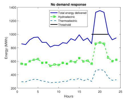
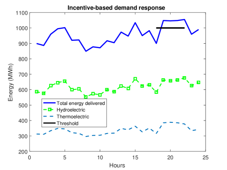
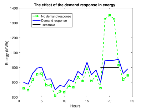
Next, Fig. 4 presents the competition case when there is an incentive command if the energy consumption is greater than the threshold $\xi=1000$ $MWh$. Below this value, the DR benefits do not apply. For instance, notice that the total energy delivered at the hour 20 is about 1351 $MWh$ in Fig. 3, i.e., above the baseline. As long as, in Fig. 4, the energy value at the same time is around 1046 $MWh$, therefore, the energy reduction is approximately 305 $MWh$ since the demand behavior is altered by the incentive payment given by the definition 6. In addition, the reduction proportion is similar for each technology. For this case, $D_{n}=25476.4\>MWh$ is used as estimated demand to solve Eq (9) and Eq. (10). Hence, the net demand is the same for both situations. If DR is employed, consumers shift energy consumption to an off period in order to maintain their satisfaction level.

4.1 The effect of demand response

In Fig. 5, the effect of DR in terms of energy is shown. Whether the consumption is higher than the threshold value ($\xi=1000\>MWh$) and if the period has reduction incentive then the DR model stimulates the consumers to reduce the energy consumption patterns. This behavior is found because the economic incentive $p_{2t}$ is introduced on the inverse demand function. Thus, this incentive payment can be understood as an alteration of consumer preferences made by SO, to alleviate the system in contingency situations where an energy reduction is required in the grid operation. For this example, the cutback during peak times is about 21.5%. This percentage changes according to the threshold selected by SO. Furthermore, demand shifts the energy requirement to other periods to hold the same activities during the day by increasing energy consumption at off-peak times.

Figure 5: The effect of the demand response in energy.

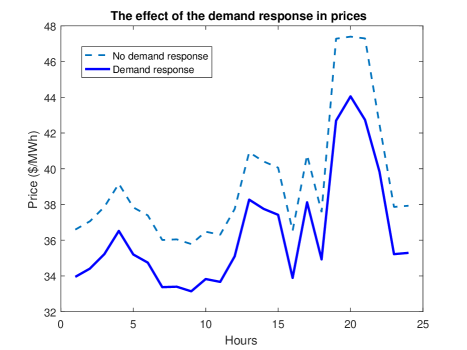
In Fig. 6, the effects of the DR in term of prices is depicted. The fashion in which a consumer reduces his energy is through economic stimulus or incentives. Under this program, consumers are rewarded by a reduction of load in peak hours. Fig. 6 shows that DR reduces the market prices since obeying the law of supply and demand for all periods. However, for obtaining the energy reduction, SO must pay an economic incentive in order to motivate the load curtailment by consumers. Therefore, in certain events, the incentive-based DR is a reasonable alternative to overcome contingency scenarios in the electric power system. At these times, it is more cost-effective to diminish demand than to increase supply or induce power outages to maintain the balance in the electrical grid.

Figure 6: The effect of demand response in prices.

4.2 Consumer and producer surplus

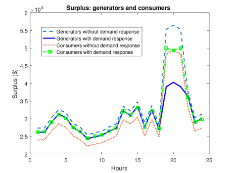
Consumer and generator surplus are shown in Fig. 7. The producer surplus is calculated from the objective functions (Eq. (5) and Eq. (8)). Whereas the consumer surplus is obtained by replacing directly the inverse demand function (4) in $\int_{0}^{q_{t}}p_{t}\left(E^{\prime}\right)dE^{\prime}-p_{t}^{*}q_{t}$. An important feature of the incentive-based DR program is that the generators decrease their profit or surplus when DR is required. This effect is due to the reduction performed by users, in which, the prices are affected by the inverse demand curve stated when the energy exceeds the threshold. Moreover, consumers are rewarded by a reduction in their energy bill whether they reduce their consumption. Therefore, users have a greater economic surplus with DR program than not participating, taking into account the previous definitions for this model.

Figure 7: Consumer and producer surplus.

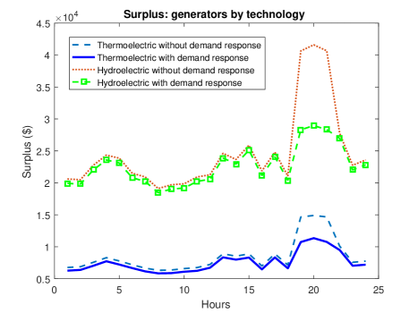
In Fig. 8, the generator surplus by technology is illustrated. Hydropower has the major participation in the electricity market, therefore, it suffers the greatest reduction in its benefits. Whereas that thermoelectric reduces slightly its profit. In general, the energy reduction depends on the participation of each generator in the energy market. For instance, 30.4% and 23.8% are the reduction percentages of hydroelectric and thermoelectric at 20 hour, respectively.

Figure 8: Generators surplus by technology.

4.3 Incentive effect in demand response

For analyzing the incentive effect in this kind of DR program, the simulation parameters are set in $\gamma_{t}=0.054\,\$/MWh^{2}$ and $\gamma_{t}\overline{q_{t}}=120.35\,\$/MWh$ for one period. Next, the aim is to change the incentive price in order to understand what happens to the energy cutback, market price, and participant surplus. In Fig. 9, the percentage energy reduction and the market price are shown according to the incentive. The immediate effect of DR is to decrease the electric power requirement and, by the law of supply and demand, the market price declines as increases the incentive signal. For instance, whether the incentive price $p_{2t}$ is equal to $10\>\$/MWh$, then the market price is $43.67\>\$/MWh$ and the energy reduction is $8.6\%$.

Figure 9: Energy reduction and market price affected by the DR incentive.

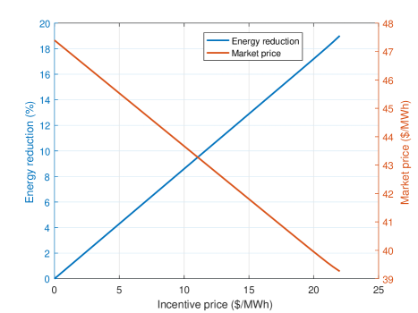
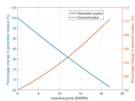
Fig. 10 illustrates the generation and demand surplus as increases the incentive price. The amount of energy to be dispatch is less when DR is required. Then, the generation profit diminishes also caused by decreasing market prices. Therefore, the main achievement of this incentive-based DR program is to guarantee the power availability in peak events or to provide a solution to a contingency situation, e.g., low water levels in reservoirs of hydroelectric power. Furthermore, consumers perceive more economic benefits when they are participating in the DR program since the net price is cheaper whether they reduce their consumption. For example, if the incentive price is 10$\$/MWh$ then users notice an increase about 3.8% of their surplus, while, the generation has a decrease around 16.1% of the profit.

Figure 10: Generation and demand surplus behavior according to the incentive price

5 Discussion

Incentive-based DR is a program where consumers receive incentive payment according to a counterfactual model, namely, they are rewarded by a price multiplied by energy reduction which is measured from household baselines. Therefore, this quantity is estimated by SO from previous energy consumption. During peak times, SO evaluates the demand forecast (baseline), power availability, transmission constraints, costs of power outages, among others in order to define if DR procedure is required.
The proposed model allows a SO to know the market behavior in an imperfect environment to take decisions when an indirect DR method is employed. This model includes a threshold which can be interpreted as a guide or reference value of the expected energy reduction during peak time at market level. In addition, the threshold can be derived or estimated from the subset of consumers that are willing to participate in DR. This information can be collected by aggregators and analyzed by SO.
Economic policy is focused on how to define the incentive signal to determine a trade-off between agent surplus, grid constraints, and market objectives. For instance, under this model, the following question could be assessed: where does the incentive come from? This could be addressed by adding a fixed cost to the market price so that it can be used to encourage consumers to reduce their energy consumption in a contingency situation. Moreover, most of the literature is concentrated on directly studying DR at distribution side without considering all effects in the system as a whole. Therefore, this model provides tools to determine choices on indirect DR methods in electricity markets.
This new price responsive demand structure is an economic tool for analyzing DR programs in imperfect markets. In addition, this approach can be extended to study the operation of centralized systems which could result in the following benefits: price responsive demand can make the power market more competitive during peak times; it also can improve the predictability of demand requirements and could provide rapid response to emergency shortage conditions; finally, it can postpone the need for generation investment and delay the need for certain transmission upgrades by decelerating the growth in peak demand.

6 Conclusions

In this work was developed an analysis of Cournot competition in an incentive-based DR program. A new demand curve was proposed for modeling consumer preferences in order to include DR in the electricity market. Incentives for consumers were considered as the DR program. The demand model was devised as a composition of two linear functions and a sigmoid, which represents an energy threshold for analyzing the load reduction in this kind of DR programs. It was found that the incentive-based DR is a cost-effective solution to reduce energy consumption during peak times. However, this program affects negatively the generator surplus under competition environment.
The proposed model can be employed to study price responsive demand in wholesale electricity markets where consumers have the opportunity to reduce voluntary their consumption according to incentive signals. Particularly, price response characteristic can enable development of enhanced operational systems to take advantage of the predictable behavior of short term consumption patterns that are associated with wholesale price conditions. For instance, the model can work as decision-making tool for grid operators to defer more expensive dispatch options and reduce transmission congestion costs.
For future works, transmission and intertemporal constraints can be incorporated into the model in order to take into account all characteristic of a dispatch problem. Additionally, a significant improvement would be to model the demand curve as a random process for studying the electrical grid behavior when renewable energies are integrated in the distribution system.