Multigrid Renormalization
Abstract
We combine the multigrid (MG) method with state-of-the-art concepts from the variational formulation of the numerical renormalization group. The resulting MG renormalization (MGR) method is a natural generalization of the MG method for solving partial differential equations. When the solution on a grid of points is sought, our MGR method has a computational cost scaling as , as opposed to for the best standard MG method. Therefore MGR can exponentially speed up standard MG computations. To illustrate our method, we develop a novel algorithm for the ground state computation of the nonlinear Schrödinger equation. Our algorithm acts variationally on tensor products and updates the tensors one after another by solving a local nonlinear optimization problem. We compare several different methods for the nonlinear tensor update and find that the Newton method is the most efficient as well as precise. The combination of MGR with our nonlinear ground state algorithm produces accurate results for the nonlinear Schrödinger equation on grid points in three spatial dimensions.
keywords:
\KWDMultigrid methods
Numerical renormalization group
Density matrix renormalization group
Variational renormalization group methods
Matrix product states
Quantics tensor trains
1 Introduction
Multigrid (MG) methods [1] are among the most efficient tools for the boundary value problem of (nonlinear) partial differential equations [2]. The standard MG method discretizes space by a finite number of grid points and provides a recipe for approaching the solution in continuous space by successively increasing . The ultimate goal of MG methods is the continuous solution which is obtained in the limit . MG methods are iterative solvers and their computational cost scales better than for others, e.g. direct solvers, namely linearly with in the best case. This allows MG methods to go to larger values of and closer to the continuum limit than alternative methods.
Around the same time when MG methods were first formulated to tackle the limit grid points in mathematics, new renormalization group (RG) techniques [3] were invented to address the limit of quantum particles in theoretical physics. The invention of the numerical renormalization group (NRG) [3] led to a breakthrough when it solved the Kondo problem – of a single magnetic quantum impurity in a nonmagnetic metal – which was an outstanding problem in condensed matter theory until then. While the NRG has proven to be a very powerful tool for a variety of quantum impurity problems [4], it has fundamental difficulties with more general quantum many-body problems such as e.g. quantum spin chains. For the latter systems, most of these difficulties could be overcome when the density matrix renormalization group (DMRG) was invented [5, 6] as a modified version of NRG – reference [7] summarizes the early success of DMRG. However, also DMRG has fundamental limitations, and many of them could be overcome when yet another key discovery was made: namely that DMRG can be equally formulated as a variational algorithm over an ansatz called matrix product states [8]. This led to new variational renormalization group (RG) methods that generalized and extended DMRG – references [9, 10, 11] cover this topic comprehensively. Note that also NRG could be improved by reformulation as a variational RG method [12, 13].
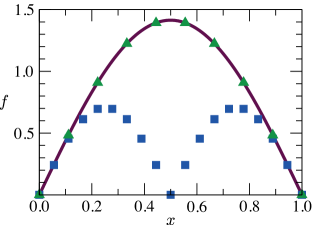
In this article, we generalize and extend the MG method by combining it with state-of-the-art concepts from variational RG methods. The resulting MG renormalization (MGR) method has a computational cost that formally scales like and can thus be exponentially faster than the MG method. Our MGR method is a natural combination of MG and variational RG methods, and it is optimal in a certain sense that we will explain later. As an example, figure 1 compares the performance of NRG and our MGR method for a free quantum particle in a box. This problem has often been used to illustrate fundamental limitations of NRG [14]. Our MGR method overcomes these limitations.
Later in this article, we will see that MGR gives rise to tensor product states. This variational ansatz is also known as tensor network states or as tensor networks in the physics community – and references [9, 10, 15] give a comprehensive overview of the physics perspective. An important subset of tensor product states is called matrix product states [8, 16, 17, 18]. These are also known as tensor train decompositions [19] or as quantics tensor train decompositions [20, 21] in the mathematics community. Here we will use existing results from the mathematics community. However, our motivation, derivations, and applications originate from a physics perspective.
It is also interesting to note that MGR produces a function representation that was originally proposed in the context of quantum computation [22, 23, 24]. There, this representation was used to show that a quantum computer achieves an exponential compression rate of lossless compression compared to a classical computer. Here, by using tensor product states, we will understand that MGR achieves an exponential compression rate of lossy compression on a classical computer.
This article is structured as follows. In section 2 we present the general MGR concept. We show how MGR naturally leads to tensor product states in subsection 2.1 and formulate the MGR method for the Poisson equation in subsection 2.2. MGR is then used to construct a new algorithm for the ground state computation of the nonlinear Schrödinger equation in section 3. There we first introduce quantities that measure the accuracy of MGR in subsection 3.1, then present our new algorithm in subsection 3.2, and finally analyse its performance in subsection 3.3.
2 Multigrid renormalization (MGR) method
In this section we present the MGR method, which is a general concept that can be applied to any (nonlinear) partial differential equation.
2.1 MGR gives rise to tensor product states
In the following we use the finite difference method to represent (nonlinear) partial differential equations. We denote the sought solution function by and assume that it is defined on the interval in each of its variables – any function can be scaled to satisfy this with all its variables. We define the vector as the values of on an equidistant grid of spacing . Furthermore each variable of shall be discretized by points, i.e. for each variable. If , , or is given explicitly then we drop the subindex in and write to simplify the notation. We first present our method for a function that depends only on one variable and later discuss the extension to more variables.
MG methods find the solution on a fine grid with the help of exact solutions from coarse grids. A crucial ingredient is the prolongation operator that maps a function from a coarse grid of spacing to a finer grid of spacing : . Usually MG methods also require a restriction operator that maps a function from a fine grid to a coarser grid [1, 2, 25] but we will not need this restriction operator here.
We now formulate an exact MG method that starts from a large grid spacing and then refines the grid in an exact way. Initially, we want to store the function values of at and in a vector . This vector lives in a two-dimensional vector space that is spanned by two basis vectors and . We define that the basis vector – where or – corresponds to on the grid. We write where the tensor has one index that takes two values or for the two components of with respect to the basis vectors and . We define a new tensor where is the same as before and takes two values, and we write any new two basis vectors in terms of the old basis vectors and . Now we decrease the grid spacing by a factor such that . For this refined grid, we want to store the function values of at , , , and in a vector . This vector lives in a four-dimensional vector space that we construct as the tensor product of the previous vector space with basis vectors and a new two-dimensional vector space with basis vectors and . We define that the basis vector – where or and or – corresponds to on the grid. We write where the tensor has one index for the previous basis and one index for the new basis. We define a new tensor where and are the same as before and takes four values, and we write any new four basis vectors in terms of the old basis vectors. We continue this procedure. In each step the grid spacing decreases by a factor of and the dimensionality of the corresponding vector grows by a factor of . Thus in step , the grid spacing reads and lives in a -dimensional vector space. We define that the basis vector – where or , or , and so on – corresponds to on the grid. We write . And we define a new tensor to write any new basis vectors .
If we want to store all the tensors , , …on our computer, we need to be aware that in step the tensor has the size , and so the required memory grows exponentially with . To prevent this from happening we now define a maximum dimensionality for the vector space spanned by the new basis vectors . The is introduced to reduce the exponential scaling to a polynomial scaling. For the initial steps there are new basis vectors, but for the later steps there are just new basis vectors. Let us denote the dimensionality of the vector space spanned by and by , where here. Then each tensor has at most the size . Therefore if we stop our procedure at step – when – our memory requirements are upper-bounded by . We refer to our new MG procedure as a MG renormalization (MGR) method because it allows us to go to much larger values of by using renormalized degrees of freedom, given by the at most -dimensional vector spaces.
Importantly, we can choose these -dimensional vector spaces in an optimal way by making use of the fact that MGR produces tensor product states. If we stop our MGR method at step we can write out the vector as
| (1) |
This is a matrix product state [8, 16, 17, 18] – also known as tensor train decomposition [19] or as quantics tensor train decomposition [20, 21] – of bond dimension . In a tensor product state, the term bond dimension denotes the maximum dimensionality of all the internal indices that connect different tensors. Figure 2 shows a graphical representation. Because MGR produces tensor product states we can reformulate finite difference approaches to (nonlinear) partial differential equations as variational algorithms over tensor product states. This allows us to make use of the plethora of already existing variational renormalization group techniques that determine the -dimensional vector spaces in an optimal way – see e.g. reference [9] and references therein.

Our MGR method uses tensor product states as a variational ansatz for the function and approaches the continuous solution via iteration of two steps: firstly minimizing a cost function and secondly prolonging to the next finer grid. The cost function is a problem-specific function . Here, we always choose the cost function for a problem in such a way that the desired solution minimizes the cost function. An example cost function is the ground state energy where denotes a Hamiltonian (e.g. from finite difference discretization of a linear Schrödinger equation). This cost function often occurs in physical problems (particularly in quantum physics) and is minimal for the exact ground state. If we are using a variational ansatz to approximate the exact ground state we can minimize the ground state energy via the variational parameters of that ansatz. Using tensor product states we minimize the cost function in the spirit of alternating least squares as proposed in reference [26]: We move from one tensor to the next and for each tensor minimize the cost function via the variational parameters of that tensor only, i.e. leaving the variational parameters of all other tensors fixed. E.g., if we are using the matrix product state of equation 1 as a variational ansatz to minimize a cost function, then we start at the tensor and minimize the cost function using only the variational parameters of . Then we move to and minimize the cost function using only the variational parameters of , then to , and so on, until , which is when we move backwards, i.e. , then , and so on, until . We repeat this procedure several times until our cost function does not change significantly anymore. In the context of tensor product states, several minimization procedures have been proposed, see e.g. references [27, 28] for methods using Monte Carlo sampling of the gradient. However, to the best of our knowledge, the alternating minimization procedure of reference [26] is the most efficient and accurate approach for the minimization of many different cost functions. And so we use this method for the minimization of all our cost functions in this article.
After minimizing the cost function of our problem, we prolong to the next finer grid. We can define our prolongation operator in many different ways. Here we define the prolongation in such a way that the new vector has the same values as on the same grid points and on the new grid points linearly interpolates between the values of on the two adjacent grid points. Expressed in terms of vector components, the prolongation operator maps the vector with components to the vector with components and . In the tensor product formalism, the operator is a tensor product operator, i.e. the generalization of the concept of tensor product states to operators. In the context of matrix product states, is a matrix product operator [29] of the form shown in figure 3. prolongs from to and is represented by a matrix product operator . The tensors have the entries , for , and , and all other tensor entries are zero. Remember that according to our notational convention the indices run from to at most whereas the and indices take values from to , as explained in figure 2. We see that our matrix product operator for has bond dimension . We prolong to approximately, by minimizing the cost function via the alternating minimization procedure of reference [29]. This approximate prolongation has a computational cost that scales like . An exact prolongation is not computationally efficient. If we were to compute exactly, then the bond dimension of would be a factor of larger than the bond dimension of . Thus, for an exact prolongation, the bond dimension doubles after each prolongation, and so grows exponentially with the number of prolongations. Remarkably, for all cases in this article, the approximation errors of our approximate prolongations turned out to be negligibly small, as we have checked explicitly.
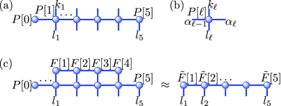
In our MGR method, we can choose among many different tensor product ansatzes for higher spatial dimensions . In this article, we simply use matrix product states with as our ansatz for all higher dimensions. Each index now represents a multi-index in two or in three spatial dimensions. And the individual indices in this multi-index specify the spatial coordinates in two or in three spatial dimensions as , , and . For the mapping from the multi-index to the single index, one usually chooses either lexicographic order – where the last index runs fastest (which corresponds to row-major order for a two-dimensional array) – or colexicographic order – where the first index runs fastest (which corresponds to column-major order for a two-dimensional array) – and in our case it is not important which order one chooses. The prolongation operators for higher spatial dimensions are obtained from the matrix product operator for one spatial dimension. We obtain the matrix product operator of bond dimension in two spatial dimensions and of bond dimension in three spatial dimensions, where denotes the Kronecker product.
2.2 MGR for the Poisson equation
The Poisson equation is a paradigmatic application for MG methods. After discretization, this equation reads where represents the Laplace operator, and boundary conditions are given, and is sought. We define the Laplace operator via the usual finite difference approximation of the second derivative from a Taylor expansion. Expressed in terms of vector components, our Laplace operator maps the vector with components to the vector with components . This finite difference approximation of the second derivative has an error that we can reduce systematically by decreasing , i.e. increasing . We choose the function on the right-hand side as a polynomial because then we know the exact solution of our Poisson equation. This allows us to analyze the performance of our MGR method by comparing to the exact solution. We choose the boundary conditions – and similarly in higher dimensions for and – as they can be implemented easily in our representation of the Laplace operator.
The Laplace operator is written as a matrix product operator as shown in figure 4, see also references [19, 20, 30]. In one spatial dimension this reads . The tensors have the entries , for , and , and all other tensor entries are zero. This matrix product operator has bond dimension . Our Laplace operators for higher spatial dimensions are constructed from this matrix product operator for one spatial dimension. We obtain the matrix product operator of bond dimension in two spatial dimensions and of bond dimension in three spatial dimensions, where denotes the identity operator for one spatial dimension.

Polynomial functions are written as matrix product states as shown in figure 5, see also references [21, 31]. We consider a polynomial of degree . After discretization, the matrix product state
for such a polynomial has bond dimension . The tensors have the entries , and for , , and all other tensor entries are zero. Here, we construct higher-dimensional polynomial functions from the matrix product state for one spatial dimension. We use in two and in three spatial dimensions. Therefore our higher-dimensional polynomials are separable products of one-dimensional polynomials, which suffice for this analysis here.

Here we compare the two cost functions and . Note that the first cost function can be written out as – where the superscript denotes transposition – and is minimal and zero for the solution of the Poisson equation. The second cost function is minimal and possibly non-zero (having the value ) for the solution of the Poisson equation. This statement is true because the gradient of with respect to is and vanishes at the minimum of such that which is the desired solution of the Poisson equation . We minimize these cost functions using the alternating minimization procedure of reference [26]. During this procedure, the tensors of our tensor product state are updated one after another and in each tensor update the cost function is minimized variationally using only the parameters of the tensor that is updated while the parameters of all the other tensors are fixed. For each tensor update, we compare the pseudoinverse, steepest descent, and conjugate gradient. The pseudoinverse has the computational cost and finds the optimal tensor parameters in one step. Steepest descent as well as conjugate gradient require steps to find the optimal tensor parameters and then their computational cost reads . With steepest descent can get very large for the convergence of each each tensor update to good tensor parameters. With conjugate gradient we make use of the fact that is positive definite – and symmetric – and then we can always find the optimal tensor parameters in each tensor update for .
The performance of the tensor train decomposition, i.e. matrix product states, in the context of the Poisson equation has been discussed in reference [32], however, without MGR. Here we want to identify the advantages of our MGR method. MGR starts from the exact solution on a coarse grid – i.e. the exact solution of the coarse grained finite difference problem – and then successively refines the grid and finds solutions on the refined grids, until the solution for the desired number of grid points is found. In this article, our MGR method always starts from and tensors with random entries, and we choose and perform alternating minimization until convergence to the exact solution. We then repeatedly implement prolongation and minimization operations, as described in section 2.1, until the desired value of has been reached. We compare our MGR method to the usual procedure which starts directly at the desired final value of , uses tensors with random entries, and then performs alternating minimization. We define that the alternating minimization procedure has converged when the relative change of the cost function is smaller than a given convergence precision. In all our numerical experiments, we observe that, for a given convergence precision, MGR converges faster than the usual procedure and to lower final values of the cost function. E.g. for convergence precision with MGR, when the conjugate gradient method is used for the tensor update, and we consider a problem in one spatial dimension with a random polynomial , we find that the number of required alternating minimization sweeps is for , for , for , for , and for . For the same convergence precision without MGR and the same problem, we find that the number of required alternating minimization sweeps is for , for , and for . Although the quantitative details of our analysis (e.g. the required number of sweeps and final value of the cost function) are problem-specific (and depend on the spatial dimensionality, , and so on), qualitatively we always observe the same: MGR improves the convergence and final result. We find that the advantages of MGR are most visible when steepest descent or conjugate gradient are used for the tensor update. In these cases, it is not possible for us to converge with the usual procedure when is larger than . In contrast, MGR converges well for all values of that we have considered, namely up to .
3 MGR for the ground state computation of the nonlinear Schrödinger equation
In this section MGR is used to develop a new algorithm for the ground state computation of the nonlinear Schrödinger equation. This equation is defined via a Hamiltonian operator that, after discretization, takes on the form
| (2) |
depends on the function that it acts upon and thus represents a nonlinear function. is the Laplace operator, represents an external potential and the interactions. Here we use this nonlinear Schrödinger equation to describe Bose-Einstein condensates and references [33, 34] provide details on the physical meaning of the individual parts of (note that equation 2 is also used in other contexts, e.g. nonlinear optics [35]). We are interested in the ground state, which is the eigenstate corresponding to the smallest possible eigenvalue in the equation .
The individual parts of in equation 2 can be written as tensor product operators. We already discussed the Laplace operator in section 2.2. We assume a simple form of the potential which, most of the time, will be a polynomial that can be constructed as explained in section 2.2. This construction gives a matrix product state for . For equation 2 we need to transform this matrix product state into a matrix product operator that has the values of the matrix product state on its diagonal. That is achieved with the help of a simple tensor which has the entries and all other entries are zero – note that this tensor is also known as the copy tensor [36, 37]. Then the construction of as a matrix product operator is straightforward as can be seen in figure 6. The interaction term needs to be constructed as a matrix product operator that has the modulus squared of the entries of on its diagonal. Using the tensor this construction is also straightforward as shown in figure 7.


3.1 Quantifying the accuracy of MGR
A standard algorithm for the ground state computation of the nonlinear Schrödinger equation is imaginary time evolution [33, 38]. In this section we use this algorithm to identify quantities for measuring the accuracy of MGR. Imaginary time evolution is based on the fact that converges to the eigenstate of corresponding to its smallest eigenvalue, i.e. the ground state, after long enough time , if the initial state is not orthogonal to that eigenstate. Note that it is important to normalize such that is true during the propagation, as otherwise the norm of can increase or decrease very quickly during imaginary time evolution. We split the total time into small time steps , i.e. , such that can be solved by applying the operator to the initial state for times. We use the approximation with an approximation error for each time step . In imaginary time evolution the propagation for the initial time steps does not need to be accurate because we are only interested in an accurate final state of the evolution. So we start the evolution with a large value of for the initial steps and then successively decrease during the evolution such that the final steps are much more accurate than the initial ones. More precisely, we start the propagation with a large value of (which is large for all , i.e. and , considered here), converge the evolved state by propagating it for large enough time steps, then decrease by a factor , converge , and so on, until all the results that we are interested in have converged. In our tensor product formalism, we find the evolved state after each time step from the state before the time step by minimizing the cost function where is defined in equation 2. We minimize this cost function by means of the alternating minimization procedure of reference [26]. Then we normalize the evolved state such that to avoid numerical problems. Thus for each time step, our time evolution algorithm has a computational cost that scales like . Note that the dominant contribution to the computational cost comes from the contraction of .
Here we only want to analyse different quantities for measuring the accuracy of MGR and so we use a particularly simple external potential in all numerical experiments of this section. Throughout this section, in equation 2, is the box potential: i.e. is everywhere inside the interval and infinitely large outside this interval.
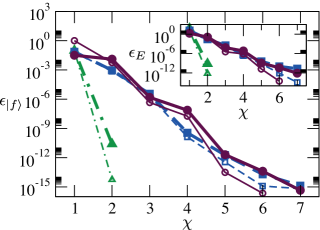
When the exact solution is known, then we can compute the infidelity and the relative energy error . Here, we compute the exact reference solution by means of imaginary time evolution of a vector of dimension which is initialized with random entries. The errors and are shown in figure 8 for several values of and . We observe that all errors decrease exponentially as a function of . Because of this numerical evidence we can thus assume an upper bound of each error where and are positive and real. This implies that, to achieve a certain error, i.e. accuracy, , we need to choose as
| (3) |
where and denote the ceiling function and we assume that such that . To gain a more intuitive understanding of equation 3, we rewrite , because we can understand as the number of digits that are correct for accuracy . Then equation 3 reads where and . We conclude that, if the error decreases exponentially as a function of , then is a linear function of , i.e. grows linearly with the number of correct digits in the solution. Equivalently, in this case, if we set the target accuracy , then the required to achieve this accuracy is a linear function of . Furthermore we can see in figure 8 that the errors do not depend significantly on . Although we only compare and (because we can only compute the exact solutions for these relatively small values of ), we can clearly expect similar error functions for larger values of from the results shown in figure 8. The fact that is independent of implies that, for a given value of we obtain the same accuracy for all possible values of , i.e. number of grid points . We conclude that tensor product states are an efficient ansatz for the problems considered here.
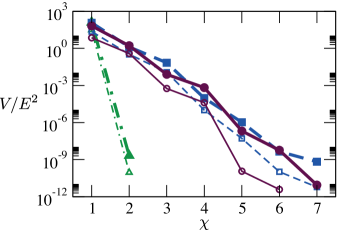
For large values of , i.e. number of grid points , we do not know and therefore cannot compute or . So we need to come up with alternative quantities to estimate the accuracy of tensor product state approximations. The normalized variance vanishes for eigenstates of . In reference [39] such a variance was used to study ground state convergence with tensor product states. Figure 9 indicates that also in our case the normalized variance can be used to analyze convergence to the ground state. However, it is important to keep in mind that this quantity measures convergence to an eigenstate which does not have to be the ground state. Furthermore, in our case the computation of has a high computational cost which is dominated by the scaling of the contraction for . This high computational cost makes the computation of the normalized variance difficult for large values of and so we will not use this quantity in the remainder of this article. Nevertheless this can be a useful quantity in the context of other (nonlinear) partial differential equations if it can be computed more efficiently there.
The quantities that we use later to analyse the accuracy of MGR follow from a transformation of our matrix product state of equation 1 into its canonical form [17, 18, 40]
| (4) |
where each matrix is diagonal with nonnegative entries that correspond to the Schmidt coefficients for the bipartition of the state between , , …, and , , …, . A general indicator for the convergence of a state with increasing is the convergence of Schmidt coefficients and von Neumann entropies for all bipartitions of the state. Notice that is also known as the entanglement entropy where . Figure 10 shows example entanglement entropies and Schmidt coefficients for some of our problems. With the help of the squared Schmidt coefficients , we can estimate the error [19, 41]
| (5) |
Although we do not know the Schmidt coefficients for , we do know them for to and can extrapolate their behavior for to . We can convince ourselves that our extrapolation is correct by increasing and checking that the new Schmidt coefficients lie on our extrapolated curve. We have thoroughly investigated this procedure of extrapolating and checking the behavior of Schmidt coefficients, and in all cases our extrapolations were very accurate. Therefore quickly decreasing Schmidt coefficients are an indicator for good accuracy of a matrix product state approximation.
Moreover, for all the problems considered here, we observe that the Schmidt coefficients for all bipartitions decrease exponentially as a function of . We thus assume that real and positive numbers and exist such that . Then the error of equation 5 has the upper bound
where and . We conclude that if all Schmidt coefficients decrease exponentially as a function of , then also the error defined in equation 5 decreases exponentially as a function of . Using equation 3, this implies that depends linearly on – where now denotes the error defined in equation 5 – and thus the required depends linearly on the number of desired correct digits.
Looking at all Schmidt coefficients is more informative than looking at just the von Neumann entropies. Quick convergence of von Neumann entropies with increasing is a necessary but not sufficient criterion for good accuracy of a matrix product state approximation [42].

3.2 Direct energy minimization via nonlinear tensor updates
Imaginary time evolution is a reliable but inefficient algorithm for ground state computation, because the ground state is obtained in an indirect way via propagation in imaginary time for typically many time steps. Direct minimization of the energy is more efficient as it aims at the ground state as directly as possible. For the nonlinear Schrödinger equation with the Hamiltonian of equation 2, the energy is for normalized functions , i.e. that fulfill . The ground state minimizes under the constraint (notice that this ground state is equivalent to the normalized eigenstate of the Hamiltonian in equation 2 corresponding to the smallest eigenvalue) [43].
We investigated several different methods for solving this constrained minimization problem from reference [44]. The method that worked best substitutes the constrained minimization problem by the unconstrained minimization of a penalty function where is a new parameter. In the limit the minimum of this unconstrained minimization problem coincides with the minimum of the original constrained minimization problem. Notice that a penalty function is a special cost function that results from replacing a constrained minimization problem by an unconstrained minimization problem and that depends on a penalty parameter in such a way that the desired solution is obtained when this penalty parameter is infinite. To compute the ground state, we therefore need to minimize for successively growing values of until the energy has converged to its smallest value and is fulfilled well enough. For each value of , we minimize via an alternating minimization procedure that sweeps over the tensors and for each tensor minimizes via the variational parameters of this tensor only, i.e. keeping the parameters of all other tensors fixed. Here each tensor update is a nonlinear optimization problem. In the following we compare steepest descent, Fletcher-Reeves conjugate gradient, Polak-Ribière conjugate gradient, and Newton method when solving the nonlinear equations. Additionally we compare the direct minimization of the penalty function with MGR and without MGR.
Our results are shown in figure 11. We observe that our MGR method converges reliably as all four methods of the nonlinear tensor update considered here converge to the same final result of within reasonable relative precisions. We take the final result of the Newton method as the reference value as it is the lowest value of . Then we obtain a relative precision of for steepest descent, for Fletcher-Reeves conjugate gradient, and for Polak-Ribière conjugate gradient. The steepest descent method requires the largest number of sweeps (more than ) for convergence and converges to the least accurate final result (i.e. the highest value of ). Both conjugate gradient methods require similar numbers of sweeps for convergence (around ) and converge to similar final results. The Polak-Ribière is a little bit faster and more precise than the Fletcher-Reeves conjugate gradient method. The Newton method requires the smallest number of sweeps for convergence and gives the most accurate final result (i.e. the lowest value of ). Notice that each time is increased by the penalty function converges to a larger value. This is not an indication of the result getting worse but arises because of the normalization of changing with .
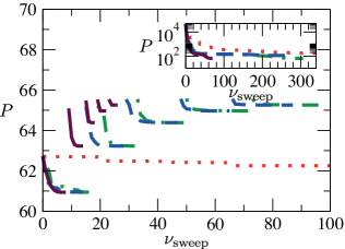
Each time is increased by , the Newton method requires approximately sweeps until convergence while each conjugate gradient method requires approximately sweeps until convergence. Firstly, this suggests that our MGR method requires a number of sweeps that grows linearly with : (notice that the accuracy of our finite discretization method grows exponentially with ). Secondly, this suggests that the Newton method converges the fastest: The computational cost of each tensor update is in the Newton method and in both conjugate gradient methods, and we performed () updates per tensor for both conjugate gradient methods and update per tensor for the Newton method. We can read off from the plot that, still, each conjugate gradient method requires approximately times more sweeps than the Newton method: Thus, in total, each conjugate gradient method needs approximately times more tensor updates than the Newton method.
We can see in the inset of figure 11 that without our MGR method no reliable convergence occurs. The four methods considered here for the nonlinear tensor update do not converge to the same values of . Both the steepest descent and the Polak-Ribière conjugate gradient method converge to relatively high values of , i.e. the methods possibly get stuck in high-lying local minima of . The Newton method achieves the lowest value of and this value coincides with the one obtained from our MGR method within a relative precision of . Without our MGR method significantly more sweeps are required for convergence than with our MGR method.
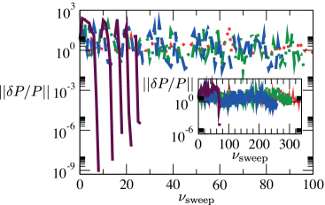
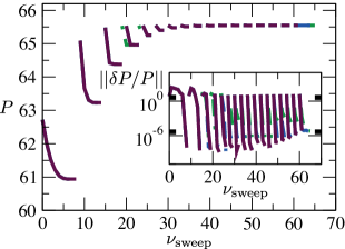
Convergence can be quantified via the norm of the normalized gradient of the penalty function . This quantity is shown in shown in figure 12. We draw the same conclusion from figure 12 as we did from figure 11: The combination that works best is MGR with the Newton method for the nonlinear tensor update. This combination is applied to a finer grid, namely , in figure 13. Figure 13 illustrates a fact that is true for all problems considered in this article: For a given convergence precision the number of sweeps required by our MGR method scales linearly with . Therefore our MGR method features an exponential speedup compared to the original MG method, namely from a computational cost scaling like to .
3.3 Performance
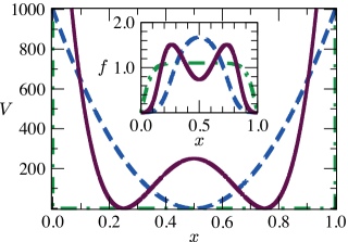
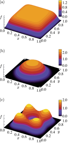
We now analyse the performance of our MGR method by computing ground states of the nonlinear Schrödinger equation in one, two, and three spatial dimensions. We consider three different external potentials: a box, a well, and a double-well. These external potentials are defined and shown for one spatial dimension in figure 14. Notice that the behavior of the solution for a double-well potential depends on the ratio between barrier height and zero-point energy of the unperturbed single-well oscillator: if the barrier is too low, then we just have a perturbed (anharmonic) single-well problem, whereas if the barrier is too high, then the problem reduces to two well-isolated single-well problems. Our double-well potential is at the cross-over between these two regimes. Our external potentials for higher spatial dimensions are constructed from the ones for one spatial dimension by taking the same potential in each dimension. E.g. the double-well potential reads in two and in three spatial dimensions, where is defined in the caption of figure 14. The corresponding matrix product operators are constructed in the same way that we used for the higher-dimensional Laplace operator in section 2.2. E.g. for the double-well potential we use in two and in three spatial dimensions, where is the matrix product operator for one spatial dimension. We choose these external potentials because the corresponding nonlinear Schrödinger equations describe Bose-Einstein condensates in laser potentials as they are currently realised in many experiments all around the world. Figures 14 and 15 illustrate how our solutions look like for one and two spatial dimensions, respectively.
We investigate the convergence of our solution function with increasing bond dimension and number of grid points in figure 16. This allows us to give precise estimates for the ground state energies in continuous space, see table 1. We observe in figure 16 that the entanglement entropy grows when the spatial dimension increases. This indicates that, to obtain a fixed accuracy for the solution, in higher spatial dimensions we need larger values of . Table 1 confirms this: For a fixed value of , the accuracy decreases with increasing spatial dimensionality. In this analysis we set the maximum to for all spatial dimensions. However, we have converged results for in one and in two spatial dimensions. For all problems considered here, we obtained machine precision of our solutions in one and two spatial dimensions. Only in three spatial dimensions, where , it is difficult to obtain converged results for because of limited computing power. Nevertheless it is remarkable that such a small value of suffices to describe grid points in three spatial dimensions and produces ground state energy accuracies that are better than one percent.

| Dimensionality | Box | Well | Double-well |
|---|---|---|---|
| 1D | 122.09942(7) | 288.05273(3) | 264.67755(3) |
| 2D | 145.0192(2) | 515.2060(2) | 444.6485(5) |
| 3D | 197.0(3) | 759.5(5) | 640(1) |
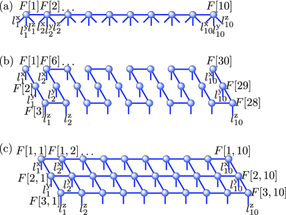
Our results in figure 16 and table 1 indicate that for higher spatial dimensions a different tensor product state ansatz might be better suited. Two alternative ansatzes are presented in figure 17. A particularly promising ansatz is the finite projected entangled pair state [45, 46] shown in figure 17 (c). This ansatz can capture much larger von Neumann entropies in higher spatial dimensions than matrix product states.
4 Conclusions and outlook
We have shown that MG methods for solving (nonlinear) partial differential equations generate functions in the form of tensor product states. Therefore these methods can alternatively be formulated as variational algorithms over tensor product states. This has the advantage that finer grids can be reached than with previous MG methods. We have constructed our MGR method as a natural combination of MG and variational renormalization group concepts. Our MGR method generalizes and extends the MG method. Moreover, our MGR method has a computational cost that scales like for grid points, whereas for the fastest previous MG methods the computational cost scales like . We have developed MGR algorithms for the linear Poisson and nonlinear Schrödinger equation. For all problems considered in this article, we have verified that the computational cost indeed scales like and, thus, our MGR method is exponentially faster than previous MG methods.
In this article, we have only used matrix product states as our tensor product state ansatz for functions in any spatial dimension. We have identified Schmidt coefficients and von Neumann entropies as useful quantifiers for the accuracy of a solution. For our ground state solutions of the nonlinear Schrödinger equation, we have often seen a significant increase of von Neumann entropies with the spatial dimension. This can be better captured by another tensor product state ansatz called projected entangled pair states [45, 46]. It would be very interesting to apply the state-of-the-art finite projected entangled pair state algorithms of references [48, 49] to partial differential equations.
In all our algorithms, we have found that the Newton method is more efficient and accurate for nonlinear tensor updates than steepest descent and conjugate gradient based approaches. This might also be the case in other tensor product state algorithms. For example, infinite projected entangled pair states [50] are composed of repeating unit cells of tensors. So far, most algorithms that use this ansatz to approximate ground states are based on imaginary time evolution. Only recently algorithms have been proposed that rely on the more efficient direct energy minimization, see e.g. references [39, 51, 52]. In this case, nonlinear tensor updates are required and we believe that the Newton method could accelerate the existing algorithms.
All problems that we have considered in this article have had relatively smooth solutions. It would be interesting to analyze the performance of our MGR method in other examples like e.g. turbulence (see e.g. reference [53] for details on how turbulence can be observed in experiments described by nonlinear Schrödinger equations). The optimal tensor product state algorithm for dynamical problems is known [54, 55]. And so it would be straightforward to analyze the performance of our MGR method for such time-dependent problems. However, there are many other interesting applications for MGR. For example, it would be exciting to apply MGR to the systematic construction of new density functionals for density functional theory, using the methods developed in reference [56]. While the scenario of reference [56] was limited to one spatial dimension and a relatively rough grid for the spatial coordinates as well as the density values, MGR can handle continuous functions in three spatial dimensions. By combining MGR with the procedure presented in reference [56], we could construct a hierarchy of successively more precise exchange-correlation energy functionals for continuous density values in three spatial dimensions: an outstanding goal in density functional theory. Another exciting future direction of research would be to address the natural question whether or not it is possible to apply our MGR method to the computation of excited states.
5 Acknowledgements
ML and DJ acknowledge funding from the NQIT (Networked Quantum Information Technologies) Hub of the UK National Quantum Technology Programme and from the EPSRC Tensor Network Theory Grant (EP/K038311/1). All tensor product algorithms of this article were programmed using the Tensor Network Theory Library [57].
References
- Brandt [1977] A. Brandt, Multi-Level Adaptive Solutions to Boundary-Value Problems, Math. Comput. 31 (1977) 333–390.
- Hackbusch [1985] W. Hackbusch, Multi-Grid Methods and Applications, Springer-Verlag (New York) (1985).
- Wilson [1975] K. G. Wilson, The renormalization group: Critical phenomena and the Kondo problem, Rev. Mod. Phys. 47 (1975) 773–840.
- Bulla et al. [2008] R. Bulla, T. A. Costi, T. Pruschke, Numerical renormalization group method for quantum impurity systems, Rev. Mod. Phys. 80 (2008) 395–450.
- White [1992] S. R. White, Density Matrix Formulation for Quantum Renormalization Groups, Phys. Rev. Lett. 69 (1992) 2863–2866.
- White [1993] S. R. White, Density-matrix algorithms for quantum renormalization groups, Phys. Rev. B 48 (1993) 10345–10356.
- Schollwöck [2005] U. Schollwöck, The density-matrix renormalization group, Rev. Mod. Phys. 77 (2005) 259–315.
- Östlund and Rommer [1995] S. Östlund, S. Rommer, Thermodynamic Limit of Density Matrix Renormalization, Phys. Rev. Lett. 75 (1995) 3537–3540.
- Verstraete et al. [2008] F. Verstraete, V. Murg, J. I. Cirac, Matrix product states, projected entangled pair states, and variational renormalization group methods for quantum spin systems, Adv. Phys. 57 (2008) 143–224.
- Cirac and Verstraete [2009] J. I. Cirac, F. Verstraete, Renormalization and tensor product states in spin chains and lattices, J. Phys. A: Math. Theor. 42 (2009) 504004.
- Schollwöck [2011] U. Schollwöck, The density-matrix renormalization group in the age of matrix product states, Ann. Phys. 326 (2011) 96–192.
- Weichselbaum et al. [2009] A. Weichselbaum, F. Verstraete, U. Schollwöck, J. I. Cirac, J. von Delft, Variational matrix-product-state approach to quantum impurity models, Phys. Rev. B 80 (2009) 165117.
- Pižorn and Verstraete [2012] I. Pižorn, F. Verstraete, Variational Numerical Renormalization Group: Bridging the Gap between NRG and Density Matrix Renormalization Group, Phys. Rev. Lett. 108 (2012) 067202.
- White and Noack [1992] S. R. White, R. M. Noack, Real-Space Quantum Renormalization Groups, Phys. Rev. Lett. 68 (1992) 3487–3490.
- Orús [2014] R. Orús, A practical introduction to tensor networks: Matrix product states and projected entangled pair states, Ann. Phys. 349 (2014) 117–158.
- Fannes et al. [1992] M. Fannes, B. Nachtergaele, R. F. Werner, Finitely correlated states on quantum spin chains, Commun. Math. Phys. 144 (1992) 443–490.
- Vidal [2003] G. Vidal, Efficient Classical Simulation of Slightly Entangled Quantum Computations, Phys. Rev. Lett. 91 (2003) 147902.
- Pérez-García et al. [2007] D. Pérez-García, F. Verstraete, M. M. Wolf, J. I. Cirac, Matrix product state representations, Quantum Inf. Comput. 7 (2007) 401–430.
- Oseledets [2011] I. V. Oseledets, Tensor-train decomposition, SIAM J. Sci. Comput. 33 (2011) 2295–2317.
- Oseledets [2010] I. V. Oseledets, Approximation of matrices using tensor decomposition, SIAM J. Matrix Anal. Appl. 31 (2010) 2130–2145.
- Khoromskij [2011] B. N. Khoromskij, -Quantics Approximation of - Tensors in High-Dimensional Numerical Modeling, Constr. Approx. 34 (2011) 257–280.
- Wiesner [1996] S. Wiesner, Simulations of Many-Body Quantum Systems by a Quantum Computer, arXiv:quant-ph/9603028v1 (1996).
- Zalka [1997] C. Zalka, Threshold Estimate for Fault Tolerant Quantum Computing, arXiv:quant-ph/9612028v2 (1997).
- Zalka [1998] C. Zalka, Simulating quantum systems on a quantum computer, Proc. R. Soc. Lond. A 454 (1998) 313–322.
- Hackbusch and Trottenberg [1982] W. Hackbusch, U. Trottenberg, Multigrid Methods, Springer-Verlag (New York) (1982).
- Verstraete et al. [2004] F. Verstraete, D. Porras, J. I. Cirac, Density Matrix Renormalization Group and Periodic Boundary Conditions: A Quantum Information Perspective, Phys. Rev. Lett. 93 (2004) 227205.
- Sandvik and Vidal [2007] A. W. Sandvik, G. Vidal, Variational Quantum Monte Carlo Simulations with Tensor-Network States, Phys. Rev. Lett. 99 (2007) 220602.
- Schuch et al. [2008] N. Schuch, M. M. Wolf, F. Verstraete, J. I. Cirac, Simulation of Quantum Many-Body Systems with Strings of Operators and Monte Carlo Tensor Contractions, Phys. Rev. Lett. 100 (2008) 040501.
- Verstraete et al. [2004] F. Verstraete, J. J. García-Ripoll, J. I. Cirac, Matrix Product Density Operators: Simulation of Finite-Temperature and Dissipative Systems, Phys. Rev. Lett. 93 (2004) 207204.
- Kazeev and Khoromskij [2012] V. A. Kazeev, B. N. Khoromskij, Low-rank explicit QTT representation of the Laplace operator and its inverse, SIAM J. Matrix Anal. Appl. 33 (2012) 742–758.
- Oseledets [2013] I. V. Oseledets, Constructive Representation of Functions in Low-Rank Tensor Formats, Constr. Approx. 37 (2013) 1–18.
- Oseledets and Dolgov [2012] I. V. Oseledets, S. V. Dolgov, Solution of linear systems and matrix inversion in the TT-format, SIAM J. Sci. Comput. 34 (2012) A2718–A2739.
- Dalfovo et al. [1999] F. Dalfovo, S. Giorgini, L. P. Pitaevskii, S. Stringari, Theory of Bose-Einstein condensation in trapped gases, Rev. Mod. Phys. 71 (1999) 463–512.
- Pitaevskii and Stringari [2003] L. Pitaevskii, S. Stringari, Bose-Einstein Condensation, Clarendon Press (Oxford) (2003).
- Scott [2005] A. Scott, Encyclopedia of Nonlinear Science, Routledge (New York) (2005).
- Al-Assam et al. [2011] S. Al-Assam, S. R. Clark, C. J. Foot, D. Jaksch, Capturing long range correlations in two-dimensional quantum lattice systems using correlator product states, Phys. Rev. B 84 (2011) 205108.
- Denny et al. [2012] S. J. Denny, J. D. Biamonte, D. Jaksch, S. R. Clark, Algebraically contractible topological tensor network states, J. Phys. A: Math. Theor. 45 (2012) 015309.
- Edwards and Burnett [1995] M. Edwards, K. Burnett, Numerical solution of the nonlinear Schrödinger equation for small samples of trapped neutral atoms, Phys. Rev. A 51 (1995) 1382.
- Vanderstraeten et al. [2016] L. Vanderstraeten, J. Haegeman, P. Corboz, F. Verstraete, Gradient methods for variational optimization of projected entangled-pair states, Phys. Rev. B 94 (2016) 155123.
- Verstraete et al. [2005] F. Verstraete, J. I. Cirac, J. I. Latorre, E. Rico, M. M. Wolf, Renormalization-Group Transformations on Quantum States, Phys. Rev. Lett. 94 (2005) 140601.
- Verstraete and Cirac [2006] F. Verstraete, J. I. Cirac, Matrix product states represent ground states faithfully, Phys. Rev. B 73 (2006) 094423.
- Schuch et al. [2008] N. Schuch, M. M. Wolf, F. Verstraete, J. I. Cirac, Entropy Scaling and Simulability by Matrix Product States, Phys. Rev. Lett. 100 (2008) 030504.
- Lieb and Yngvason [1998] E. H. Lieb, J. Yngvason, Ground State Energy of the Low Density Bose Gas, Phys. Rev. Lett. 80 (1998) 2504.
- Griva et al. [2009] I. Griva, S. G. Nash, A. Sofer, Linear and Nonlinear Optimization, 2nd edition, Soc. Indust. Appl. Math. (Philadelphia) (2009).
- Verstraete and Cirac [2004] F. Verstraete, J. I. Cirac, Renormalization algorithms for quantum many-body systems in two and higher dimensions, arXiv:cond-mat/0407066v1 (2004).
- Murg et al. [2007] V. Murg, F. Verstraete, J. I. Cirac, Variational study of hard-core bosons in a two-dimensional optical lattice using projected entangled pair states, Phys. Rev. A 75 (2007) 033605.
- Stoudenmire and White [2012] E. M. Stoudenmire, S. R. White, Studying Two-Dimensional Systems with the Density Matrix Renormalization Group, Annu. Rev. Cond. Matt. Phys. 3 (2012) 111–128.
- Lubasch et al. [2014a] M. Lubasch, J. I. Cirac, M.-C. Bañuls, Unifying projected entangled pair state contractions, New J. Phys. 16 (2014a) 033014.
- Lubasch et al. [2014b] M. Lubasch, J. I. Cirac, M.-C. Bañuls, Algorithms for finite projected entangled pair states, Phys. Rev. B 90 (2014b) 064425.
- Jordan et al. [2008] J. Jordan, R. Orús, G. Vidal, F. Verstraete, J. I. Cirac, Classical Simulation of Infinite-Size Quantum Lattice Systems in Two Spatial Dimensions, Phys. Rev. Lett. 101 (2008) 250602.
- Corboz [2016] P. Corboz, Variational optimization with infinite projected entangled-pair states, Phys. Rev. B 94 (2016) 035133.
- Liu et al. [2017] W.-Y. Liu, S.-J. Dong, Y.-J. Han, G.-C. Guo, L. He, Gradient optimization of finite projected entangled pair states, Phys. Rev. B 95 (2017) 195154.
- Navon et al. [2016] N. Navon, A. L. Gaunt, R. P. Smith, Z. Hadzibabic, Emergence of a turbulent cascade in a quantum gas, Nature 539 (2016) 72–75.
- Lubich et al. [2015] C. Lubich, I. V. Oseledets, B. Vandereycken, Time integration of tensor trains, SIAM J. Numer. Anal. 53 (2015) 917–941.
- Haegeman et al. [2016] J. Haegeman, C. Lubich, I. V. Oseledets, B. Vandereycken, F. Verstraete, Unifying time evolution and optimization with matrix product states, Phys. Rev. B 94 (2016) 165116.
- Lubasch et al. [2016] M. Lubasch, J. I. Fuks, H. Appel, A. Rubio, J. I. Cirac, M.-C. Bañuls, Systematic construction of density functionals based on matrix product state computations, New J. Phys. 18 (2016) 083039.
- Al-Assam et al. [2017] S. Al-Assam, S. R. Clark, D. Jaksch, The tensor network theory library, J. Stat. Mech.: Theor. Exp. 2017 (2017) 093102.