Distribution Matching in Variational Inference
Mihaela Rosca Balaji Lakshminarayanan Shakir Mohamed {mihaelacr,balajiln,shakir}@google.com
DeepMind
Abstract
With the increasingly widespread deployment of generative models, there is a mounting need for a deeper understanding of their behaviors and limitations. In this paper, we expose the limitations of Variational Autoencoders (VAEs), which consistently fail to learn marginal distributions in both latent and visible spaces. We show this to be a consequence of learning by matching conditional distributions, and the limitations of explicit model and posterior distributions. It is popular to consider Generative Adversarial Networks (GANs) as a means of overcoming these limitations, leading to hybrids of VAEs and GANs. We perform a large-scale evaluation of several VAE-GAN hybrids and analyze the implications of class probability estimation for learning distributions. While promising, we conclude that at present, VAE-GAN hybrids have limited applicability: they are harder to scale, evaluate, and use for inference compared to VAEs; and they do not improve over the generation quality of GANs.
1 INTRODUCTION
This paper focuses on the challenges of training Variational Autoencoders (VAEs) (Kingma and Welling, 2013, Rezende et al., 2014): the struggles of matching the marginal latent posterior distribution with the prior, the difficulties faced in explicitly specifying latent posteriors, and the lack of likelihoods that capture the semantic similarity of data. To overcome the limitations of VAEs, it has become natural to consider borrowing the strengths of another popular type of generative algorithm, Generative Adversarial networks (GANs) (Goodfellow et al., 2014), resulting in a fusion of VAEs and GANs (Mescheder et al., 2017, Srivastava et al., 2017, Makhzani et al., 2015, Larsen et al., 2016, Rosca et al., 2017, Pu et al., 2017). What are the limitations of VAEs at present? How can GANs help? Do VAE-GAN hybrids address the limitations currently being experienced? The aim of this paper is to offer an answer to these questions.
Generative models currently have a wide range of applications in dimensionality reduction, denoising, reinforcement learning, few-shot learning, data-simulation and emulation, semi-supervised learning and in-painting (Smith, 2002, Mathieu et al., 2016, Higgins et al., 2017b, Rezende et al., 2016, Kingma et al., 2014, Salimans et al., 2017, Nguyen et al., 2016), and they continue to be deployed in new domains, from drug-discovery to high-energy physics. It thus becomes vital for us to explore their strengths and shortcomings, and deepen our understanding of the performance and behavior of generative models.
We will contrast conditional distribution matching in VAEs with marginal distribution matching in VAE-GAN hybrids. We compare the performance of explicit distributions in VAEs with the use of implicit distributions in VAE-GAN hybrids. And we measure the effect of distributional assumptions on what is learned. We will make the following contributions:
-
•
We show that VAEs fail to match marginal distributions in both latent and visible space and that powerful explicit model distributions and powerful explicit posteriors do not improve marginal distribution matching in VAEs. This is prevalent across datasets, models and latent dimensionality.
-
•
We systematically evaluate existing and new VAE-GAN hybrids as promising avenues to improve variational inference, but show that since they use classifier probabilities to estimate density ratios and learn implicit distributions, they lack an accurate estimate for the likelihood bound that can be used for model evaluation and comparison.
-
•
We uncover the effect of marginal distribution matching in latent space on latent representations and learned posterior distributions, and show that VAE-GAN hybrids are harder to scale to higher latent dimensions than VAEs.
These contributions will lead us to conclude that while VAE-GAN hybrids allow for posterior inference in implicit generative models, at present, VAE-GAN hybrids have limited applicability: compared to VAEs, their use of classifier probabilities makes them harder to scale, evaluate, and use for inference; compared to GANs, they do not improve sample generation quality.
2 CHALLENGES WITH VAES
One goal of generative models is to match the unknown distribution of data to the distribution learned by a model. In latent variables models, is defined via a latent variable and the hierarchical model:
| (1) |
The integral in Equation 1 for computing is, in general, intractable, making it hard maximize the marginal likelihood of the model under the data, . To overcome this intractability, variational inference introduces a tractable lower bound on via a variational distribution :
| (2) | |||
| (3) |
The training objective is to learn the model parameters of the distribution and the variational parameters of to maximize the evidence lower bound (ELBO):
| (4) |
Distributions and can be parametrized using neural networks and trained jointly using stochastic gradient descent as in Variational Autoencoders (Kingma and Welling, 2013, Rezende et al., 2014). In this setting, we refer to as the encoder distribution, and to as the decoder distribution.
The ideal learning scenario does marginal distribution matching, in visible space: matching to the true data distribution . Variational inference, using a lower bound approximation, achieves this indirectly using conditional distribution matching in latent space: minimizing in Equation 2 and searching for a tight variational bound.
Marginal distribution matching in visible space, and conditional distribution matching in latent space, are tightly related through marginal distribution matching in latent space By doing a “surgery on the ELBO”, Hoffman and Johnson (2016) showed how variational inference methods minimize when maximizing the ELBO, since:
| (5) | ||||
The integral in (5) is a mutual information and is non-negative. Minimizing therefore minimizes a lower bound on , i.e. matching the marginal distributions.
There are two reasons to be interested in marginal distribution matching. Firstly, we can unveil a failure to match to , and to in VAEs. This failure can be associated to the use of conditional distribution matching and explicit distributions. Our goal will be to explore the solutions to overcome these failures provided by marginal distribution matching and implicit models. Secondly, the marginal divergence can be used as a metric of VAE performance since it captures simultaneously two important characteristics of performance: the ability of the learned posterior distribution to match the true posterior, and the ability of the model to learn the data distribution.
An alternative examination of VAEs as a rate-distortion analysis, achieved by using a coefficient in front of the KL term in the ELBO (e.g., Higgins et al. (2017a)), is the closest to our work. Alemi et al. (2017) show that simple decoders have a smaller KL term but have high reconstruction error, whereas complex decoders are better suited for reconstruction. Their investigation does not consider implicit distributions and alternative approaches to distribution matching, and is complementary to this effort.
3 QUANTIFYING VAE CHALLENGES
To motivate our later exploration of marginal distribution matching and implicit distribution in variational inference, we first unpack the effects of conditional distribution matching and explicit distributions. We show that VAEs are unable to match the marginal latent posterior to the prior . This will result in a failure to learn the data distribution, and manifests in a discrepancy in quality between samples and reconstructions from the model. To the best of our knowledge, no other extensive study has been performed showing the prevalence of this issue across data sets, large latent sizes, posterior and visible distributions, or leveraged this knowledge to generate low posterior-probability VAE samples. Hoffman and Johnson (2016) initially showed VAEs with Gaussian posterior distributions, Bernoulli visible distribution and a small number of latents trained on binary MNIST do not match and .
We train VAEs with different posterior and model distributions on ColorMNIST (Metz et al., 2017), CelebA (Liu et al., 2015) at 64x64 image resolution, and CIFAR-10 (Krizhevsky, 2009). Throughout this section, we estimate via Monte Carlo using (pseudocode in Appendix E).
3.1 Effect of latent posterior distribution
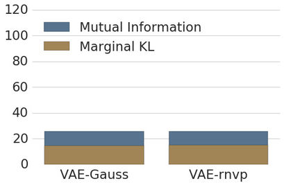
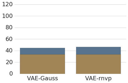
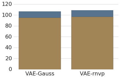
Powerful explicit posteriors given by Real Non Volume Preserving (RNVP) normalizing flows (Dinh et al., 2016) do not improve marginal distribution matching in VAEs over simple diagonal Gaussian posteriors. This result, shown in Figure 1 which reports for trained VAEs, is surprising given that RNVP posteriors are universal distribution approximators, and have the capacity to fit complex posteriors and perhaps suggests that posterior distributions are not the biggest bottleneck in VAE training.
3.2 Effect of the visible distribution
The choice of visible distribution also affects distribution matching in latent space. We trained the same VAE architecture using Bernoulli and Quantized Normal visible distributions on CIFAR-10. A Quantized Normal distribution is a normal distribution with uniform noise added to discrete pixel data (Theis et al., 2016). Since a Bernoulli distribution provides the same learning signal as a QuantizedNormal with unit variance (formal justification in Appendix G), the QuantizedNormal distribution has a higher modeling capacity, leading to better data reconstructions. However, this does not result an increased sample quality: better reconstructions force to encode more information about the data, making the KL between and the data agnostic higher, thus increasing the gap between sample and reconstruction quality. Apart from visually assessing the results (see Appendix G), we can now quantify the different behavior using , which is 44.7 for a Bernoulli model, and 256.7 for the same model with a QuantizedNormal distribution. We saw similar results when comparing Categorical and Bernoulli distributions.
3.3 Low probability posterior samples
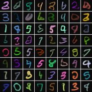
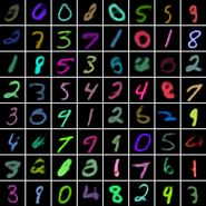
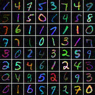
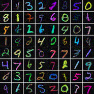
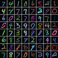
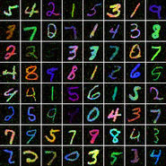
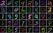
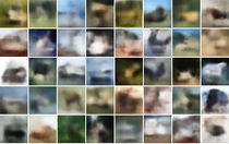
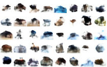
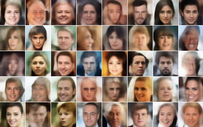
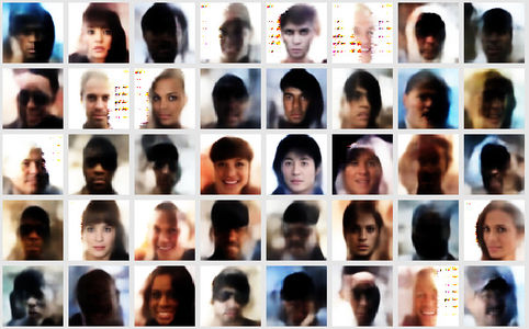
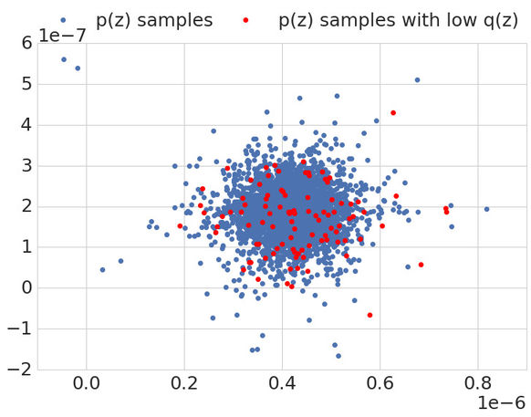
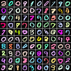
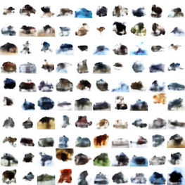
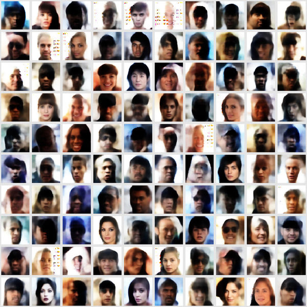
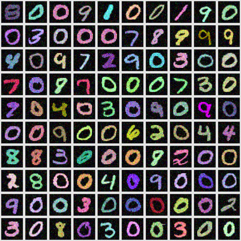
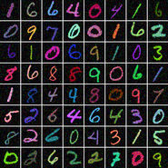
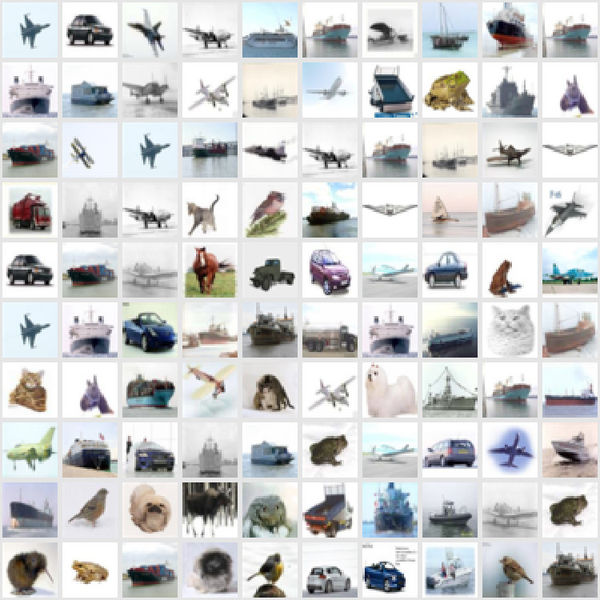
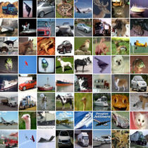
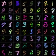
We exploit the failure of VAEs to match marginal distributions in latent space to purposefully generate ‘bad’ samples: samples obtained from prior samples that have low probability under the marginal posterior . Such bad samples, shown in Figure 2, exhibit common characteristics such as having thickened-lines for ColorMNIST and strong white backgrounds for CelebA and CIFAR-10. We can look at where in latent space the samples with low probability under the marginal are. Figure 3 (right) is a t-SNE visualisation which shows that the latents which generate the low posterior VAE samples in Figure 2 are scattered throughout the space of the prior and not isolated to any particlar regions, with large pockets of prior space which are not covered by .
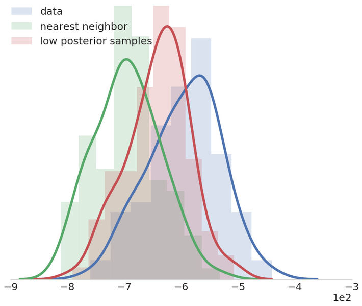
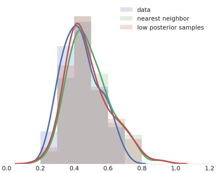
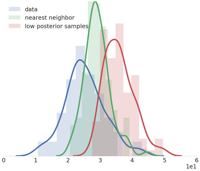
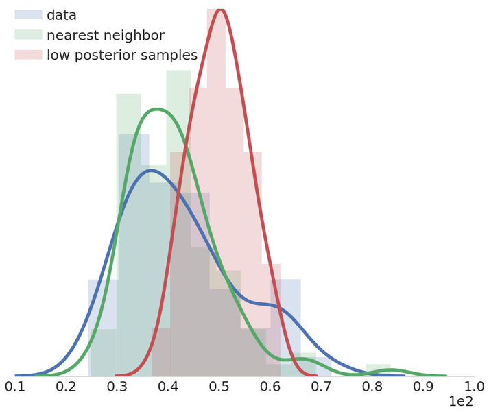
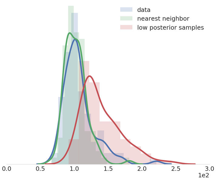
Since these ‘bad’ samples are unlikely under the true distribution, we expect a well trained model to distinguish easily, using the likelihood bound, typical images (which come from the data) from atypical samples (generated from regions of the marginal distribution with low-probability). Figure 3 (left) shows that on ColorMNIST the model recognizes that the low posterior samples and their nearest neighbors have a lower likelihood than the data, as expected. But for CIFAR-10 and CelebA the model thinks the low posterior samples are more likely than the data, despite the samples being quantitatively and qualitatively different (see Appendix A for more samples and metrics).
The latent space spread of low posterior samples, together with the inability of VAEs to learn a likelihood that reflects the data distribution, show a systematic failure of these models to match distributions in latent and visible space.

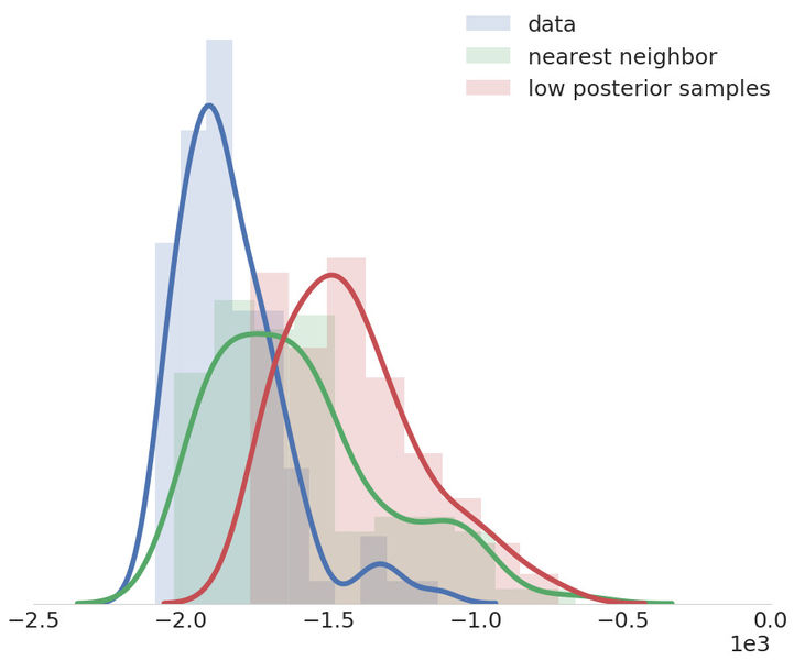
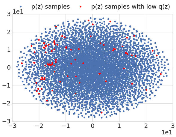
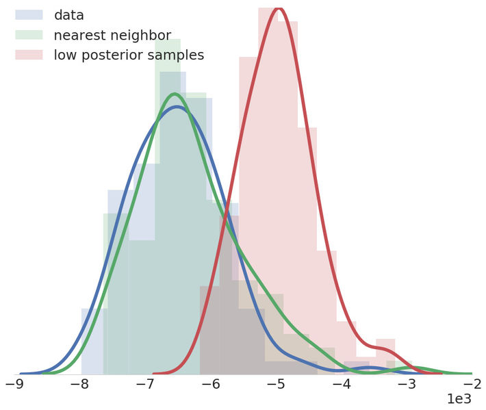
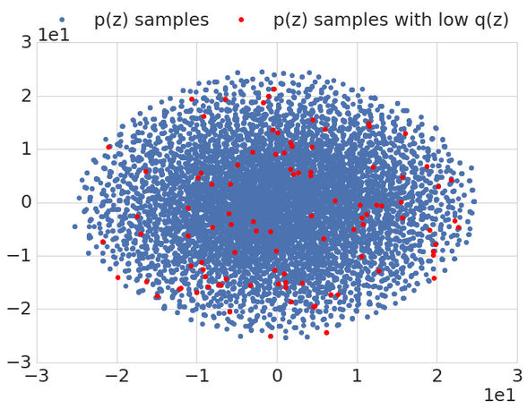
.
4 GANS IN LATENT SPACE
If it is conditional divergence minimization and explicit posteriors that result in a failure of VAEs to match marginal distributions, then we are strongly motivated to explore other approaches . We turn to another popular type of algorithm, generative adversarial networks (GANs), and explore the density ratio trick, which they use as a tool for marginal distribution matching and implicit distributions in variational inference, leading to VAE-GAN hybrids.
4.1 Distribution matching with density ratios
The density ratio trick (Sugiyama et al., 2012, Goodfellow et al., 2014, Goodfellow, 2014) leverages the power of classifiers in order to estimate density ratios. Under the assumption that we can train a perfect binary classifier to associate the label to samples from and the label to samples from , the following holds:
| (6) |
Conveniently, this approach only requires distribution samples, without the explicit forms of the two
distributions. GANs (Goodfellow et al., 2014) use the density ratio trick to directly match the data distribution
with the marginal model distribution . By making use of implicit latent variable
models (Mohamed and Lakshminarayanan, 2016) GANs do not require observation likelihoods - they define by
specifying a deterministic mapping used to generate model samples. GANs learn
via an adversarial game, using a discriminator to distinguish between generated samples and real data. In
the original formulation, the training was given by the min-max bi-level optimization with value
function111In all our experiments we use the alternative non-saturating generator loss
(Goodfellow et al., 2014).:
When the density ratio trick is used for learning - like in GANs - the ratio estimator cannot be trained to optimality for each intermediate model distribution, since this would be computationally prohibitive. In practice, the model and the estimator are trained jointly using alternating gradient descent (Goodfellow et al., 2014, Fedus et al., 2018). Since KL divergences are an expectation of density ratios, the density ratio trick opens the door to implicit posteriors and marginal distribution matching in latent space for variational inference.
Implicit variational posteriors. The choice of posterior distribution in VAEs is limited by the use of the choice of in . Since the density ratio trick only requires samples to estimate , it avoids restrictions on and opens the door to implicit posteriors. However, replacing each KL divergence in equation 4 with a density ratio estimator is not feasible, as this requires an estimator per data point. AdversarialVB (Mescheder et al., 2017) solves this issue by training one discriminator to estimate all ratios for by distinguishing between pairs and .
Marginal distribution matching. Since conditional distribution matching fails to match marginal distributions in latent and visible space, directly minimizing provides a compelling alternative. Adversarial Autoencoders (AAE) (Makhzani et al., 2015) ignore the mutual information term in Equation 5 and minimize using adversarial training. AAEs are connected to marginal distribution matching not only by the ELBO, but also via Wasserstein distance (Tolstikhin et al., 2018) (see Appendix C).
4.2 Effects of density ratios on evaluation, scalability and latent representations
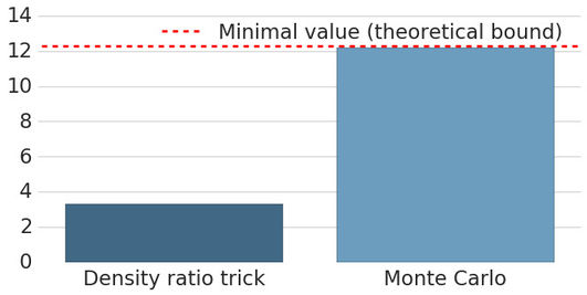
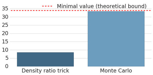
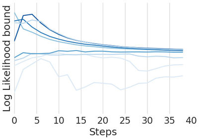
Evaluation. Using the density ratio trick in variational inference comes at a price: the loss of an estimate for the variational lower bound. Leveraging binary classifiers to estimate KL divergences results in underestimated KL values, even when the discriminator is trained to optimality (see Figure 4). This issue is exacerbated in practice, as the discriminator is updated online during training. By using density ratios, VAE-GAN hybrids lose a meaningful estimate to report and a quantity to use to assess convergence, as shown in Figure 5. While VAEs can be compared with other likelihood models, VAE-GAN hybrids can only use data quality metrics for evaluation and lack a metric that can used to track model convergence.

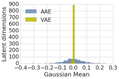
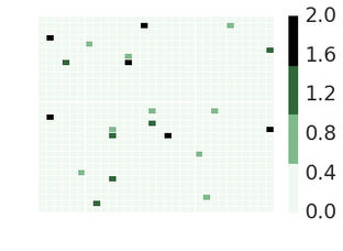
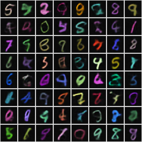
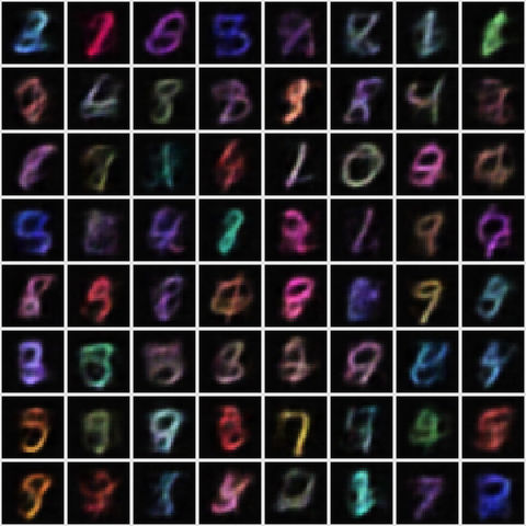
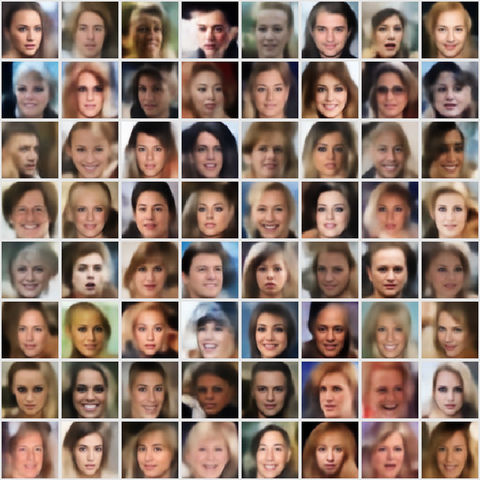
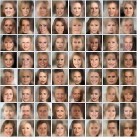
Scalability is another concern when using the density ratio trick. Using synthetic experiments where the true KL divergence is known, we show that using classifiers to provide learning signal does not scale with data dimensions (Appendix D). In practice this can be observed by training VAEs and AAEs with 1000 and 10000 latents. While VAEs learn to ignore extra latents (Figure 6) and scale with no architectural changes to extra dimensions, AAEs struggle to model ColorMNIST and completely fail on CelebA even with a bigger discriminator – see Figures 16 and 17 in Appendix B.
Latent representations learned via marginal divergence minimization have different properties than representations learned with VAEs. Figure 6 contrasts the posterior Gaussian means learned using AAEs and VAEs with 1000 latents on ColorMNIST: VAEs learn sparse representations, by using only a few latents to reconstruct the data and ignoring the rest, while AAEs learn dense representations. This is a consequence of marginal distribution matching: by not having a cost on the conditional , AAEs can use any posterior latent distribution but lose the regularizing effect of - when learning a Gaussian the variance collapses to 0 and the mean has a much wider range around the prior mean compared to VAEs. This finding suggests that for downstream applications such as semi supervised learning, using VAE representations might have a different effect compared to using representations learned by VAE-GAN hybrids.
5 GANS IN VISIBLE SPACE
The benefits and challenges of marginal distribution matching and implicit distributions in variational inference go beyond matching distributions in latent space. Using implicit models for the data avoids notorious problems with explicit likelihoods, such as blurry samples and reconstructions produced by common choices such as Gaussian or Laplacian distributions. To introduce marginal distribution matching in variational inference, we introduce a ratio in the likelihood term of (4):
| (7) |
denotes the entropy of and can be ignored for optimization purposes. This approach is a form of synthetic likelihood (Wood, 2010, Dutta et al., 2016).
Equation (7) shows the challenges of replacing the likelihood term with a density ratio:
-
1.
Naively using the density ratio trick requires an infinite number of discriminators, one for each with .
-
2.
The model no longer receives gradients, since the parametric estimator replacing is evaluated at data points, as given by the expectations in Equation 7. The model has been absorbed by the ratio estimator - by providing samples to it.
To avoid both problems and continue analyzing the effects of marginal distribution matching in variational inference, we leverage GANs to train the generative model. A previously proposed solution explores joint distribution matching (Srivastava et al., 2017, Dumoulin et al., 2017, Donahue et al., 2017, Li et al., 2017).
5.1 Marginal distribution matching
To bypass Equation (7), instead of using conditional distribution matching done when maximizing the ELBO, we use a ratio estimator to distinguish between and the marginal reconstruction distribution . The loss function for the ratio estimator becomes:
| (8) |
To produce realistic reconstructions which fool the discriminator, the encoder and decoder minimize an adversarial loss, such as . This approach to marginal distribution matching in visible space can be used in conjunction with either conditional or marginal matching in latent space and lends itself to training both implicit and explicit models.
When learning explicit models, marginal distribution matching and conditional distribution matching as done in variational inference can be combined. From the variational inference view the adversarial loss acts as a regularizer, steering reconstructions towards an area of the space that makes them realistic enough to fool the discriminator. From the adversarial perspective, the reconstruction loss can be viewed as a regularizer which avoids mode collapse, a notorious issue with GANs Srivastava et al. (2017), Arjovsky et al. (2017).
All VAE-GAN hybrids discussed so far rely on the KL term to match distributions in latent space. Adversarial training in visible space gives us another way to match and , by matching the data distribution and the model distribution, via a discriminator which minimizes:
| (9) |
The decoder now receives an adversarial loss both for reconstructions and samples, learning how to produce compelling looking samples from early on in training, like GANs. Unlike GANs, this model is able to do inference, by learning . We will later show that this loss helps improve sample quality compared to using an adversarial loss only on reconstructions, as described in equation 8.
5.2 Joint variants
Matching joint distributions matches both visible and latent space distributions. Minimizing divergences in the joint space leads to solutions for lack of gradients and challenges of density ratio estimation of Equation 7 while staying completely in the variational inference framework, by changing the goal of the model and using a different variational bound. VEEGAN Srivastava et al. (2017) changes the model objective from matching the marginals and in data space to matching marginal distributions in latent space. Using a reconstructor network to learn a posterior distribution , the goal of VEEGAN is to match to the prior . Because is intractable, is introduced as a variational distribution using the lower bound:
where is a constant. The model is trained to minimize the negative of the lower bound and a reconstruction loss in latent space. To estimate , VEEGAN uses the density ratio trick - and hence also loses an estimate for the bound – Appendix H. Since the expectation in the objective is not taken with respect to the data distribution but the joint distribution decoder gradients follow from the variational objective.
6 EVALUATION
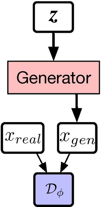
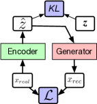
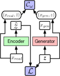
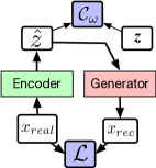
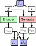
We compare marginal distribution matching using implicit distributions in variational inference provided by VAE-GAN hybrids with VAEs and GANs on image generation tasks. We perform an extensive comparison between (detailed in Figure 7):
-
•
VAEs with diagonal Gaussian posteriors – the most widespread variational inference model.
-
•
DCGAN and WGAN-GP to provide a baseline for VAE-GAN hybrids.
-
•
AAE to exhibit the effect of replacing the analytical KL in VAEs with the density ratio trick.
-
•
VEEGAN to evaluate the density ratio trick on joint distributions, and the effect of reconstruction losses in latent space rather than data space.
-
•
VGH and VGH++, two Variational GAN Hybrids we introduce inspired by the analysis in Section 5.1. Like AAEs, these models use marginal distribution matching in latent space via the density ratio trick. In visible space, VGH uses a discriminator trained on reconstructions (Equation 8), and VGH++ uses a discriminator trained on both data and samples (Equation 9). Both use an reconstruction loss in data space. Details are provided in Appendix 5. Contrasting VGH and AAEs measures the effect of explicit distribution matching in visible space, while comparing VGH and VGH++ assesses the efficacy of the density ratio trick in latent space.
We do not compare with AdversarialVB, as it underperformed in our initial experiments (Appendix J). Other approaches to VAE-GAN hybrids include replacing reconstruction losses on pixels with reconstruction losses on discriminator features (Larsen et al., 2016), but they are outside the scope of this work.
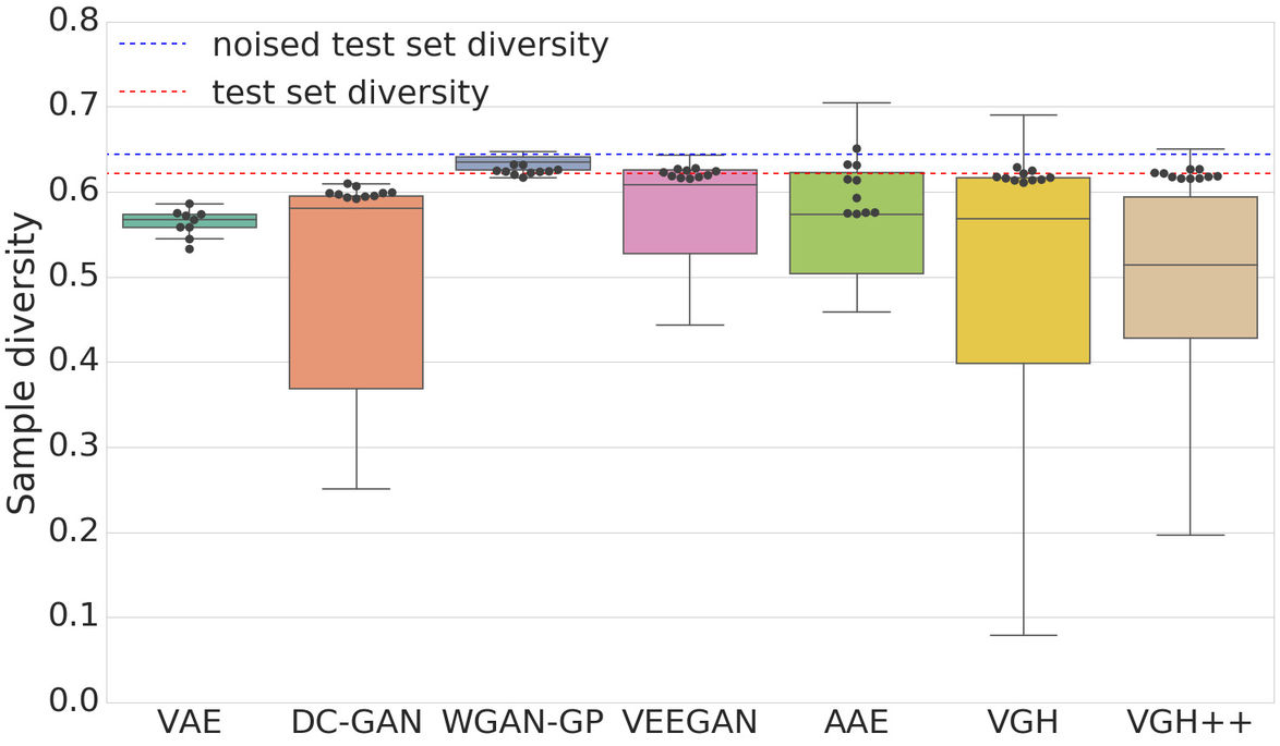
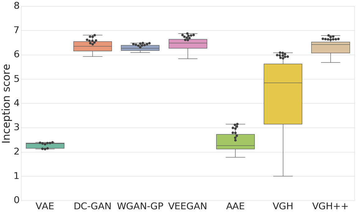
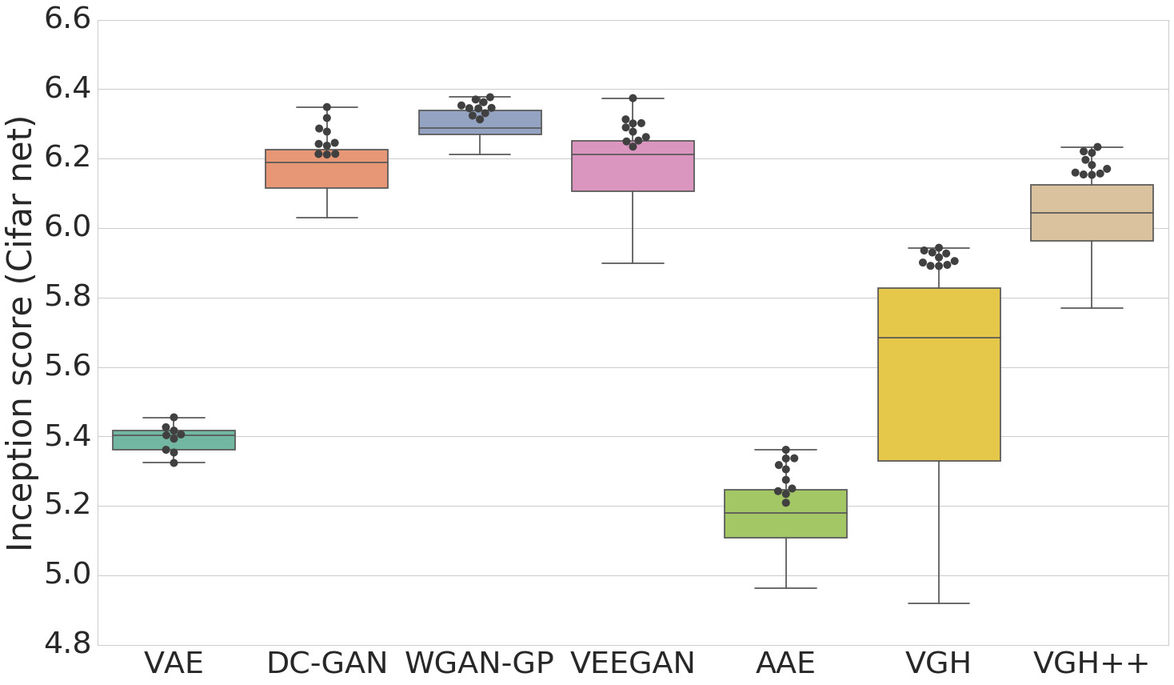
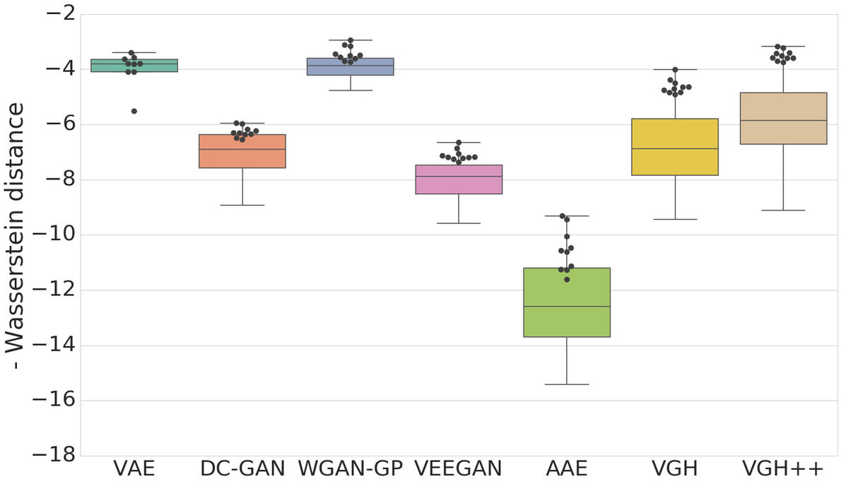
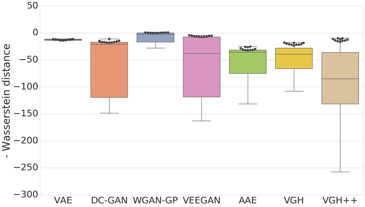
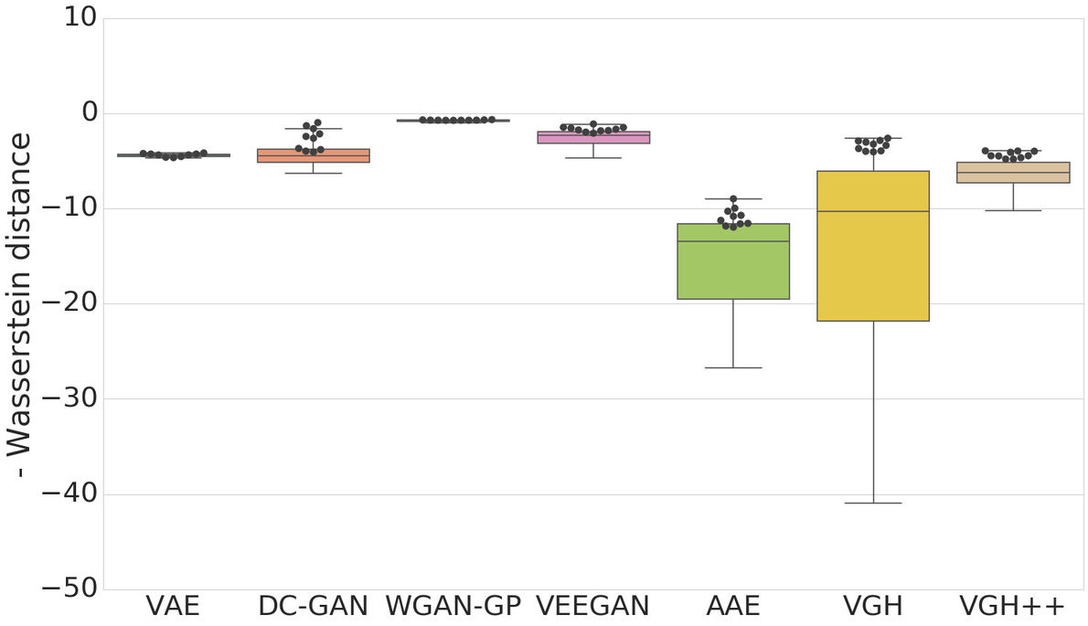
We train models on ColorMNIST, CelebA and CIFAR-10 and complement visual inspection of samples with three metrics: Inception Score, sample diversity, independent Wasserstein critic. We do not use the ELBO as an evaluation metric, since we have shown VAE-GAN hybrids cannot estimate it reliably. Descriptions of the metrics, experimental details and samples are in Appendices I, K and M.
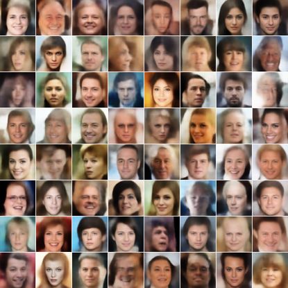
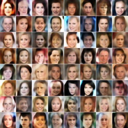
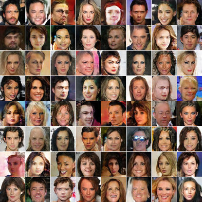
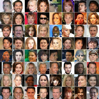
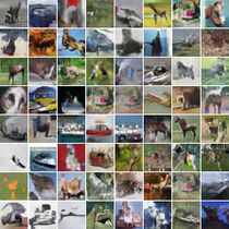
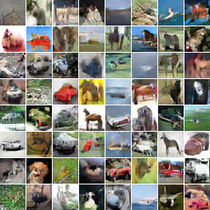
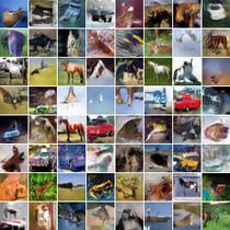
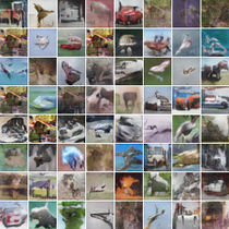
Figures 8 and 9 show that VAEs perform well on datasets that have less variability, such as ColorMNIST and CelebA, but are not able to capture the subtleties of CIFAR10. Marginal distribution matching in visible space improves generation quality, with VEEGAN, VGH++ and VGH performing better than VAEs and AAEs. However, VAE-GAN hybrids do not outperform GANs on image quality metrics and consistently exhibit a higher sensitivity to hyperparameters, caused by additional optimization components. VGH++ consistently outperforms VGH, showing that the density ratio trick has issues matching the marginal latent posterior to the prior and that matching marginal distributions in visible space explains the increased sample quality of VAE-GAN hybrids compared to VAEs.
By assessing sample quality and diversity, our experiments show that, at present, merging variational inference with implicit and marginal distribution matching does not provide a clear benefit.
7 CONCLUSION
We have shown the widespread failure to learn marginal distributions with Variational Autoencoders. We asked whether this is the effect of conditional distribution matching, and of explicit posteriors and explicit model distributions. To test this hypothesis, we explored marginal distribution matching and implicit distribution in variational inference, through existing and new VAE-GAN hybrids.
Through a wide range of experiments, we have shown that VAE-GAN hybrids do not deliver on the promise of addressing major challenges in variational inference. Problems with value estimation of divergences caused by the use of classifier probabilities, difficulties of scaling to high dimensions, hyperparameter sensitivity and the struggles to outperform GANs on sample quality metrics, limits, at present, the applicability of VAE-GAN hybrids. Since implicit models and adversarial training do not solve the obstacles of variational inference, distribution matching in latent and visible space remain important generative models research issues.
References
- Alemi et al. (2017) A. A. Alemi, B. Poole, I. Fischer, J. V. Dillon, R. A. Saurous, and K. Murphy. An information-theoretic analysis of deep latent-variable models. arXiv preprint arXiv:1711.00464, 2017.
- Arjovsky et al. (2017) M. Arjovsky, S. Chintala, and L. Bottou. Wasserstein GAN. In ICML, 2017.
- Danihelka et al. (2017) I. Danihelka, B. Lakshminarayanan, B. Uria, D. Wierstra, and P. Dayan. Comparison of Maximum Likelihood and GAN-based training of Real NVPs. arXiv preprint arXiv:1705.05263, 2017.
- Dinh et al. (2016) L. Dinh, J. Sohl-Dickstein, and S. Bengio. Density estimation using Real NVP. arXiv preprint arXiv:1605.08803, 2016.
- Donahue et al. (2017) J. Donahue, P. Krähenbühl, and T. Darrell. Adversarial feature learning. In ICLR, 2017.
- Dumoulin et al. (2017) V. Dumoulin, I. Belghazi, B. Poole, A. Lamb, M. Arjovsky, O. Mastropietro, and A. Courville. Adversarially learned inference. In ICLR, 2017.
- Dutta et al. (2016) R. Dutta, J. Corander, S. Kaski, and M. U. Gutmann. Likelihood-free inference by penalised logistic regression. arXiv preprint arXiv:1611.10242, 2016.
- Fedus et al. (2018) W. Fedus, M. Rosca, B. Lakshminarayanan, A. M. Dai, S. Mohamed, and I. Goodfellow. Many paths to equilibrium: GANs do not need to decrease a divergence at every step. In ICLR, 2018.
- Goodfellow et al. (2014) I. Goodfellow, J. Pouget-Abadie, M. Mirza, B. Xu, D. Warde-Farley, S. Ozair, A. Courville, and Y. Bengio. Generative adversarial nets. In NIPS, 2014.
- Goodfellow (2014) I. J. Goodfellow. On distinguishability criteria for estimating generative models. arXiv preprint arXiv:1412.6515, 2014.
- Gulrajani et al. (2017) I. Gulrajani, F. Ahmed, M. Arjovsky, V. Dumoulin, and A. Courville. Improved training of Wasserstein GANs. In NIPS, 2017.
- Guo et al. (2017) C. Guo, G. Pleiss, Y. Sun, and K. Q. Weinberger. On calibration of modern neural networks. In ICML, 2017.
- Higgins et al. (2017a) I. Higgins, L. Matthey, A. Pal, C. Burgess, X. Glorot, M. Botvinick, S. Mohamed, and A. Lerchner. -VAE: Learning basic visual concepts with a constrained variational framework. In ICLR, 2017a.
- Higgins et al. (2017b) I. Higgins, A. Pal, A. A. Rusu, L. Matthey, C. P. Burgess, A. Pritzel, M. Botvinick, C. Blundell, and A. Lerchner. DARLA: Improving zero-shot transfer in reinforcement learning. In ICML, 2017b.
- Hochreiter and Schmidhuber (1997) S. Hochreiter and J. Schmidhuber. Long short-term memory. Neural computation, 9(8):1735–1780, 1997.
- Hoffman and Johnson (2016) M. D. Hoffman and M. J. Johnson. ELBO surgery: yet another way to carve up the variational evidence lower bound. In Workshop in Advances in Approximate Bayesian Inference, NIPS, 2016.
- Ioffe and Szegedy (2015) S. Ioffe and C. Szegedy. Batch normalization: Accelerating deep network training by reducing internal covariate shift. In ICML, 2015.
- Jiwoong Im et al. (2018) D. Jiwoong Im, A. He Ma, G. W. Taylor, and K. Branson. Quantitatively evaluating GANs with divergences proposed for training. ICLR, 2018.
- Kingma and Ba (2015) D. Kingma and J. Ba. Adam: A method for stochastic optimization. In ICLR, 2015.
- Kingma and Welling (2013) D. P. Kingma and M. Welling. Auto-encoding variational Bayes. In ICLR, 2013.
- Kingma et al. (2014) D. P. Kingma, S. Mohamed, D. J. Rezende, and M. Welling. Semi-supervised learning with deep generative models. In NIPS, 2014.
- Kos et al. (2017) J. Kos, I. Fischer, and D. Song. Adversarial examples for generative models. arXiv preprint arXiv:1702.06832, 2017.
- Krizhevsky (2009) A. Krizhevsky. Learning multiple layers of features from tiny images. 2009.
- Larsen et al. (2016) A. B. L. Larsen, S. K. Sønderby, H. Larochelle, and O. Winther. Autoencoding beyond pixels using a learned similarity metric. In ICML, 2016.
- Li et al. (2017) C. Li, H. Liu, C. Chen, Y. Pu, L. Chen, R. Henao, and L. Carin. Alice: Towards understanding adversarial learning for joint distribution matching. In Advances in Neural Information Processing Systems, pages 5501–5509, 2017.
- Liu et al. (2015) Z. Liu, P. Luo, X. Wang, and X. Tang. Deep learning face attributes in the wild. In ICCV, 2015.
- Maas et al. (2013) A. L. Maas, A. Y. Hannun, and A. Y. Ng. Rectifier nonlinearities improve neural network acoustic models. In ICML, 2013.
- Makhzani et al. (2015) A. Makhzani, J. Shlens, N. Jaitly, I. Goodfellow, and B. Frey. Adversarial autoencoders. arXiv preprint arXiv:1511.05644, 2015.
- Mathieu et al. (2016) M. F. Mathieu, J. J. Zhao, J. Zhao, A. Ramesh, P. Sprechmann, and Y. LeCun. Disentangling factors of variation in deep representation using adversarial training. In NIPS, 2016.
- Mescheder et al. (2017) L. Mescheder, S. Nowozin, and A. Geiger. Adversarial Variational Bayes: Unifying Variational Autoencoders and Generative Adversarial Networks. In ICML, 2017.
- Metz et al. (2017) L. Metz, B. Poole, D. Pfau, and J. Sohl-Dickstein. Unrolled generative adversarial networks. In ICLR, 2017.
- Mohamed and Lakshminarayanan (2016) S. Mohamed and B. Lakshminarayanan. Learning in implicit generative models. arXiv preprint arXiv:1610.03483, 2016.
- Nguyen et al. (2016) A. Nguyen, J. Yosinski, Y. Bengio, A. Dosovitskiy, and J. Clune. Plug & play generative networks: Conditional iterative generation of images in latent space. arXiv preprint arXiv:1612.00005, 2016.
- Odena et al. (2016) A. Odena, C. Olah, and J. Shlens. Conditional image synthesis with auxiliary classifier GANs. arXiv preprint arXiv:1610.09585, 2016.
- Papamakarios et al. (2017) G. Papamakarios, I. Murray, and T. Pavlakou. Masked autoregressive flow for density estimation. In NIPS, 2017.
- Pu et al. (2017) Y. Pu, W. Wang, R. Henao, L. Chen, Z. Gan, C. Li, and L. Carin. Adversarial symmetric variational autoencoder. In NIPS, 2017.
- Rezende et al. (2016) D. Rezende, I. Danihelka, K. Gregor, D. Wierstra, et al. One-shot generalization in deep generative models. In ICML, 2016.
- Rezende et al. (2014) D. J. Rezende, S. Mohamed, and D. Wierstra. Stochastic backpropagation and approximate inference in deep generative models. In ICML, 2014.
- Rosca et al. (2017) M. Rosca, B. Lakshminarayanan, D. Warde-Farley, and S. Mohamed. Variational approaches for auto-encoding generative adversarial networks. arXiv preprint arXiv:1706.04987, 2017.
- Salimans et al. (2017) T. Salimans, I. Goodfellow, W. Zaremba, V. Cheung, A. Radford, and X. Chen. Improved techniques for training GANs. In NIPS, 2017.
- Smith (2002) L. I. Smith. A tutorial on principal components analysis. Technical report, 2002.
- Srivastava et al. (2017) A. Srivastava, L. Valkov, C. Russell, M. Gutmann, and C. Sutton. VEEGAN: Reducing mode collapse in GANs using implicit variational learning. In NIPS, 2017.
- Sugiyama et al. (2012) M. Sugiyama, T. Suzuki, and T. Kanamori. Density-ratio matching under the Bregman divergence: a unified framework of density-ratio estimation. Annals of the Institute of Statistical Mathematics, 64(5):1009–1044, 2012.
- Szegedy et al. (2016) C. Szegedy, V. Vanhoucke, S. Ioffe, J. Shlens, and Z. Wojna. Rethinking the inception architecture for computer vision. In CVPR, 2016.
- Theis et al. (2016) L. Theis, A. van den Oord, and M. Bethge. A note on the evaluation of generative models. In ICLR, 2016.
- Tolstikhin et al. (2018) I. Tolstikhin, O. Bousquet, S. Gelly, and B. Schoelkopf. Wasserstein auto-encoders. In ICLR, 2018.
- Wang et al. (2003) Z. Wang, E. P. Simoncelli, and A. C. Bovik. Multiscale structural similarity for image quality assessment. In Conference Record of the Thirty-Seventh Asilomar Conference on Signals, Systems and Computers, 2004., volume 2, pages 1398–1402. IEEE, 2003.
- Wood (2010) S. N. Wood. Statistical inference for noisy nonlinear ecological dynamic systems. Nature, 466(7310):1102–1104, 2010.
Appendix –Distribution Matching in Variational Inference
Appendix A Low posterior VAE samples
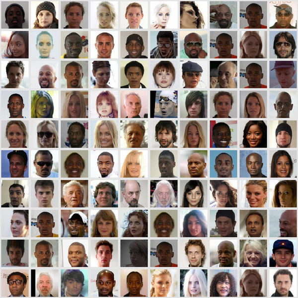
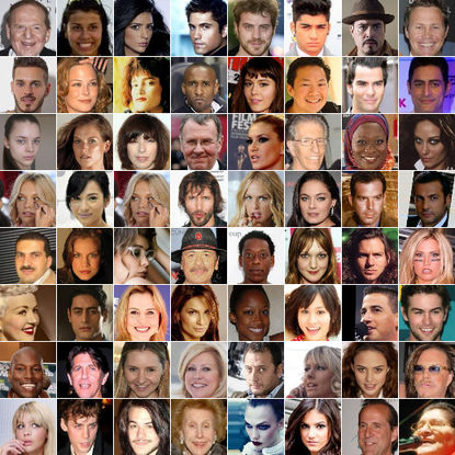
In this section we detail the experiments performed to create low posterior VAE samples. For the algorithm used to obtained the low posterior samples, see Algorithm 1. For the low posterior samples alongside standard samples from the model, see Figure 10.



A.1 Low posterior samples - model analysis
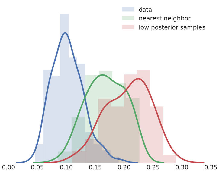
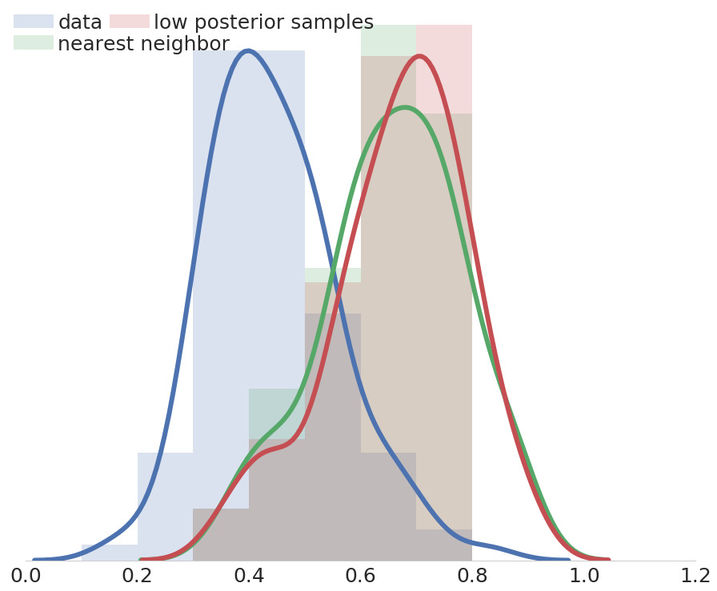
In order to understand why the low posterior samples look as shown in Figure 10, we performed an analysis to show how these samples compare to the data distribution. For ColorMNIST, we visually saw that the samples are thicker than the data or the standard samples, while for CelebA and CIFAR-10 we saw predominantly white backgrounds so we plotted the pixel histogram of the dataset against the pixel histogram of the low posterior samples (Figure 12). The histograms of pixels for data, low posterior samples and their nearest neighbors in the dataset shows that the low posterior samples differ in pixel composition compared to the uniformly sampled data, but to check whether images like this exist in the dataset we plot the nearest neighbors in distance from the dataset to the low posterior samples (see Figure 11). This analysis shows that data examples that are similar to the low posterior samples exist, but based on the histogram analysis and visual inspection we know that they have low probability under the true data distribution. A hypothesis emerges: the model is not putting mass in the marginal posterior distribution for areas of the space that encode data points which have low probability under the true data distribution. To test this hypothesis, we report the histograms of average , obtained by encoding data sampled from the dataset uniformly compared to the nearest neighbors of the low posterior samples Engineering Retreat Googl examples and the low posterior samples themselves (Figure 13). Our results show that indeed, the data points closest to the low posterior samples have a higher KL cost compared to datapoints sampled uniformly from the dataset and that these data points are unlikely under the data distribution. Knowing that these examples are unlikely under the true data distribution, we expect to see the same under the model distribution. In Figure 14 we show that for CIFAR-10 and CelebA, the model reports that the low posterior samples are more likely than the data. This demonstrated that the model is unable to capture the subtleties of the data distribution, and can be fooled into predicting high likelihoods for samples that have low probability under the true data distribution. In this work we have exploited the gap between the prior and marginal posterior distributions in VAEs trained with Gaussian posteriors, to show that the model can generate samples are far from the sample distribution and far from the data distribution. Previous work has focused on finding adversarial examples as input to the VAE by finding points in data space that the VAE is unable to reconstruct (Kos et al., 2017).






Appendix B Scaling up latent spaces in VAEs and AAEs
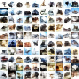
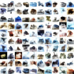
Figure 16 shows that VAEs scale better than AAEs to a high number of latent size - in this case 10000.


Appendix C Connection to Wasserstein Autoencoders
Tolstikhin et al. (2018) prove the connection between using optimal transport to minimize the distance the true data distribution and the model distribution induced by an implicit model and using autoencoders which minimize a distance between the marginal posterior and prior in latent space. Specifically, they show that:
Theorem 1
Let be a measurable cost function with values in and the set of all joint distributions with marginals and , respectively.
For a model where is a Dirac delta function, ie. is mapped to deterministically , the following holds:
| (10) |
Theorem 1 shows that for implicit models, encoder-decoder models can be introduced as a way to make the optimal transport computation tractable, as optimizing over the space of joint distributions is not feasible - another approach to make the computation tractable, when is a metric, is to use the Kantorovich-Rubinstein duality Arjovsky et al. (2017).
Similarly, when doing maximum likelihood - minimizing the KL divergence between the model and data distribution - encoder-decoder models are introduced to overcome the intractability introduced by Equation 1, using Jensen’s inequality (Equation 3).
The connections between optimal transport and maximum likelihood do not stop here - Tolstikhin et al. (2018) optimize the RHS of Equation 1 using a relaxation that adds a penalty to the objective which forces the marginal close to :
| (11) |
When setting to the or distance (corresponding to a Gaussian or Laplacian likelihood in the explicit model case), and setting to the KL divergence, we obtain the bound obtained by doing the ELBO surgery performed on the maximum likelihood objective and the training objective used to train Adversarial Autoencoders.
Hence under certain conditions, optimal transport and maximum likelihood problems lead to encoder-decoder architecture and similar optimization criteria, but allow for different modeling choices. In variational inference, the choice of in decides the reconstruction cost function, while in Wasserstein Autoencoders has to be a Dirac delta function, but the reconstruction cost is chosen by the practitioner. Like Adversarial Autoencoders, by approximating using the density ratio trick or the Wasserstein GAN objective, Wasserstein Autoencoders lose a meaningful quantity to track - which is not the case for Variational Autoencoders which use the closed form of the KL divergence.
The connection between optimal transport and maximum likelihood opens new avenues for research that we leave for future work, while the different modeling choices provide new flexibility to machine learning practitioners.
Appendix D Learning with density ratios: synthetic data experiments
We show that the density ratio trick can be used for learning, even though it cannot be used for estimating divergences. We also show the challenges of scaling the density ratio trick to higher dimensions. To do so, devise a set of synthetic experiments where the true KL divergence is known and where we can determine how this approach scales with data dimensionality.
We use Gaussian distributions, defined by passing a random normal vector through an affine transformation with :
| (12) |
To ensure is full rank, we set in all our experiments.
We first train a classifier to distinguish between two such Gaussian distributions, for varying values of . In the first setting, we are concerned with divergence estimation, keeping both distributions fixed and only learn the density ratio using the classifier. Once the classifier is trained, we report the difference between the estimated and true KL divergence values. In the second setting, we are concerned with divergence minimization and we begin with the same initialization for the two distributions, but learn the parameters of the second Gaussian ( and in Equation 12) to minimize the estimated divergence between the two distributions. This is a GAN training regime, where the generator loss is given by the reverse KL generator loss (Mohamed and Lakshminarayanan, 2016): . We track the true KL divergence during training together with the online classifier estimated divergence - we should not expect the latter to be accurate, the classifier is not trained to optimality for each update of the learned distribution, as the two models are trained jointly.
If for the same classifier that failed to approximate the true KL divergence in the estimation experiments we observe a decrease in true divergence in the learning experiments, we can conclude that while the density ratio trick might not be a useful for estimation, it can still be used as an optimization tool. To ensure our conclusions are valid, we control over hyper-parameters, classifier architectures and random seeds of the Gaussian distributions, and average results over 10 runs.
Our main findings are summarized in Figures 18, 19, and 20 and reveal that using density ratios for learning does not reliably scale with data dimensionality. For lower dimensional data (1 and 10 dimensions), the model is able to decrease the true KL divergence. However, for higher dimensional Gaussians (dimensions 100 and 1000), a classifier with 100 million parameters (4 layer MLP) is not able to provide useful gradients and learning diverges (rightmost plot in Figure 2). Regardless of data dimensionality, the estimate of the true KL divergence provided by the density ratio trick was not accurate.
The discriminator was trained with the AdamOptimizer with set to 0.5 and set to 0.9 for 1000000 iterations. Unless otherwise specified, the discriminator was a 4 layer MLP, trained with a learning rate of . The learning rate used for learning the Gaussian was . Similar results were obtained for different learning rates for the discriminator and the linear model of the Gaussian distribution.


Appendix E Estimating
E.1 Estimating using the Monte Carlo approach
Algorithm 2 describes the approach used to estimate via Monte Carlo methods. While this approach is computationally expensive, it the most accurate one. We now describe the details of this computation. For each we used samples from to estimate . To estimate for latent sample we used the entire dataset training and validation split of the dataset at hand. In all our figures and tables, this number is reported as .
E.2 Estimating using the density ratio trick
To estimate using the density ratio trick as shown in Figure 4 we used Algorithm 3. For all datasets, we noticed that this approach is highly sensitive to hyperparameters. We explain this two fold: first, this approach relies on the probabilities reported by a neural network classifier, which have been known to be inaccurate. New methods have been proposed to address this issue (Guo et al., 2017), and we leave exploring these approaches for future work. Second, as shown in Section E.3, the distribution can be very complex, making it hard for the classifier to learn to distinguish between samples from the two distributions.
We show the hyperparameter sensitivity by training different models to estimate the marginal for the same VAE and report the different values obtained. All trained density ratio estimators were MLPs with Leaky Rectified activations of slope 0.2 and were trained for steps using the AdamOptimizer with and equal to 0.9.
While analyzing these results, we observed that adding noise to the activation of the classifier resulted in a better classifier, but also a more confident one, which underestimates the probability that a sample was given by the prior, and the KL value being over estimated. We also see that the resulting KL is quite sensitive to the the architecture of the classifier, with an extra layer resulting in a substantial value increase for the Color MNIST case. Gradients penalties and dropout did not result in a big change in the estimated value.
| # layers | Gradient Penalty | Activation Noise | KL |
|---|---|---|---|
| No | No | 2.3 | |
| No | No | 3.3 | |
| No | Yes | 25812.8 | |
| Yes | No | 3.1 |
| # layers | Learning Rate | Activation Noise | Dropout | KL |
|---|---|---|---|---|
| 0.0005 | No | No | 17.7 | |
| 0.0005 | Yes | No | 720140.9 | |
| 0.0001 | No | No | 14.8 | |
| 0.0005 | No | No | 18.8 | |
| 0.0005 | No | Yes | 19.0 | |
| 0.0001 | No | No | 18.0 | |
| 0.0001 | No | No | 18.1 |
E.3 Estimating using a density model for
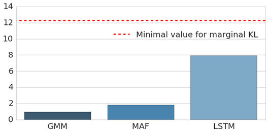
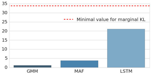
We compare the MonteCarlo and density ratio trick approach with a third way to estimate : by using a density model to learn . We use three density models: Gaussian Mixture Model, Masked Auto-regressive Flows (Papamakarios et al., 2017), and Gaussian auto-regressive models implemented using an (Hochreiter and Schmidhuber, 1997). Algorithm 4 was used to learn these models. Across models, we show a failure (see Figure 21) to reach the theoretical bound, showing that is a complex distribution.
Diagonal Gaussian Mixture Models
In this setting, we model using:
Masked Auto-regressive Flows
In this setting, the density model is given by transforming a standard Gaussian using auto-regressive models as normalizing flows:
where has to be an invertible function for which the determinant of its Jacobian is easy to compute. In practice, we leverage the fact that the composition of two functions which have these proprieties also has this property to chain a number of transforms.
Gaussian Auto-regressive models
The auto-regressivity of the recurrent neural network was used to model :
Appendix F VGH++ loss function and pseudocode
In all the equations below, refers to the data discriminator, while refers to the code discriminator. They are both trained to minimize a cross entropy loss, like in the original GAN formulation.
The loss function for VGH is:
In contrast, the loss function for VGH++ is:
The overall training procedure is summarized in Algorithm 5.
data reconstruction and code generation loss
| (13) |
data reconstruction and generation loss
treat data as real, reconstructions and samples as fake
treat as real and codes from the encoder as fake
| (14) |
Appendix G The effect of the visible distribution in VAE training
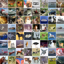
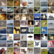
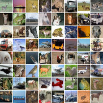
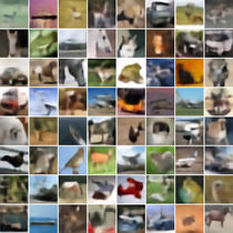
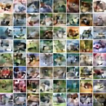
Figure 22 visually shows the trade-off seen between using a Bernoulli or a QuantizedNormal distribution as the visible pixel distribution, in VAEs.
We now unpack the mathematical justification for why the Bernoulli distribution produces worse reconstructions. We will perform the analysis for a pixel , but this straightforwardly extends to entire images. Assume a Bernoulli distribution with mean . Then the Bernoulli loss is . The gradient of the loss is , where is the sigmoid function. If we use a Gaussian distribution with mean and standard deviation , the gradient is . We can see that the gradients of the two distributions have the same form, and using a Bernoulli distribution is equivalent to using a Gaussian distribution with variance 1. By setting the variance to 1, using a Bernoulli likelihoods spreads mass around each pixel and cannot specialize to produce good reconstructions.

Appendix H Tracking the variational lower bound - VEEGAN
In this section we compare the evidence lower bound training behavior, between VAEs and VEEGAN. VEEGAN introduces a new bound,
| (15) |
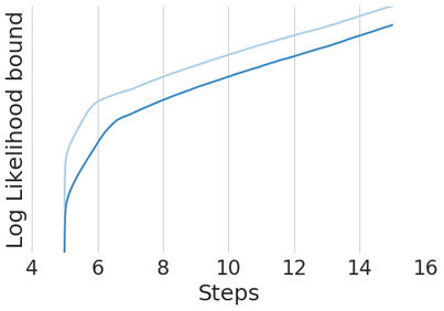
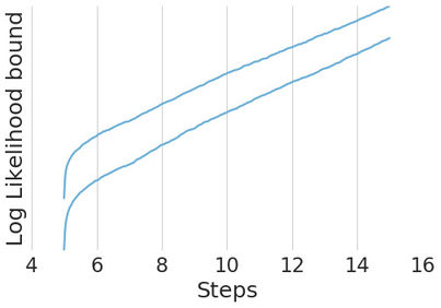
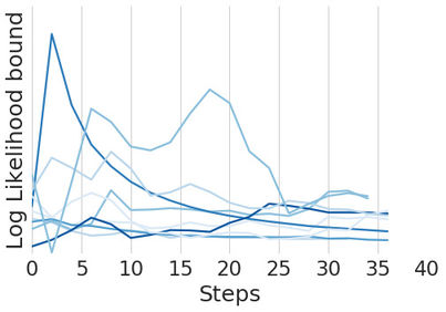
where is the reconstructor network used to build the implicit and the KL divergence is estimated using the density ratio trick. The expected and desired behavior is that the bound increases as training progresses, however, as seen in Figure 23, variational hybrids do not solve one of the fundamental problems with adversarial model training, namely introducing a quantity to use to assess convergence.
Appendix I Real data evaluation metrics
A universal metric that can assess both overfitting, sample quality and sample diversity has not been found for generative models. Instead, multiple metrics which assess different aspects of a model have been proposed. To get a better overview of model performance, we use metrics which each capture a different aspect of training.
Inception score - sample quality and between class sample diversity: The most popular evaluation metric for implicit models is the Inception Score (Salimans et al., 2017). The Inception Score correlates with human sample evaluation and measures sample quality, between class sample diversity, but cannot capture withing class mode collapse (for example, the model could generate the same horse again and again, and the Inception Score will not penalize it) or overfitting. The Inception score uses the last layer logits of a ImageNet trained Inception network (Szegedy et al., 2016) to determine how classifiable a sample is. For generative models trained on CIFAR10, we complement our reporting by using a VGG style convolutional neural network, trained on CIFAR10, which obtained 5.5% error.
Multi-scale structural similarity (MS-SSIM): sample diversity: To measure sample diversity, we use 1.0 - MS-SSIM (Wang et al., 2003), an image similarity metric ranging between 0.0 (low similarity) and 1.0 (high similarity) that has been shown to correlate well with human judgment. The use of MS-SSIM for sample diversity was introduced by Odena et al. (2016), which used it compute in class sample similarity for conditional models, as between class variability can lead to ambiguous results. For models trained on the CelebA dataset, we can use this sample diversity metric, since the dataset only contains faces.
Independent Wasserstein critic - sample quality and overfitting: Danihelka et al. (2017) and Jiwoong Im et al. (2018) proposed training an independent Wasserstein GAN critic to distinguish between real data and generated samples. This metric has been shown to correlate with human evaluations (Jiwoong Im et al., 2018), and if the independent critic is trained on validation data, it can also be used to measure overfitting (Danihelka et al., 2017). All our reported results using the Independent Wasserstein Critic use a WGAN-GP model, trained to distinguish between the data validation set and model samples.
Appendix J AdversarialVB results
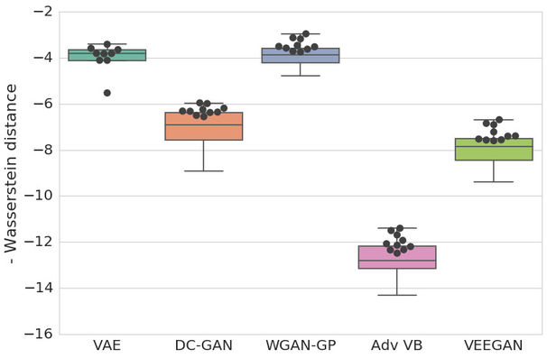
Results obtained using AdversarialVB are presented in Figure 24.
Appendix K Training details: hyperparameters and network architectures
For all our models, we kept a fixed learning rate throughout training. We note the difference with AGE, where the authors decayed the learning rate during training, and changed the loss coefficients during training222As per advice found here: https://github.com/DmitryUlyanov/AGE/.). The exact learning rate sweeps are defined in Table 3. We used the Adam optimizer (Kingma and Ba, 2015) with and and a batch size of 64 for all our experiments. We used batch normalization (Ioffe and Szegedy, 2015) for all our experiments. We trained all ColorMNIST models for 100000 iterations, and CelebA and CIFAR-10 models for 200000 iterations.
| Network | VAE |
|
AAE |
|
VEEGAN | ||||
|---|---|---|---|---|---|---|---|---|---|
| Generator/Encoder | |||||||||
| Discriminator | — | — | |||||||
| Code discriminator | — | — | — |
Scaling coefficients
We used the following sweeps for the models which have combined losses with different coefficients (for all our baselines, we took the sweep ranges from the original papers):
-
•
WGAN-GP
-
–
The gradient penalty of the discriminator loss function: 10.
-
–
-
•
VGH++ and VGH
-
–
Data reconstruction loss for the encoder: sweep over 1, 5, 10, 50.
-
–
Data reconstruction loss for the generator: sweep over 1, 5, 10, 50.
-
–
Adversarial loss for the generator (coming from the data discriminator): 1.0.
-
–
Adversarial loss for the encoder (coming from the code discriminator): 1.0.
-
–
For Adversarial Autoencoders and VEEGAN, we followed the advice from the original paper and did not weight the different loss terms using coefficients.
Choice of loss functions
For VEEGAN, we used the loss as the code reconstruction loss. For VGH and VGH++ , we used as the data reconstruction loss and the classifier GAN loss for the data and code discriminator.
Updates
For the WGAN-GP experiments, we did 5 discriminator updates for generator update. All other models used the same number updates for model component (discriminator, generator, encoder, decoder).
Choice of latent prior
We use a univariate normal prior for all models.
K.1 Network architectures
For all our baselines, we used the same discriminator and generator architectures, and we controlled the number of latents for a fair comparison. For methods which needs an encoder such as VAEs, VEEGAN, VGH and VGH++ , the encoder is always set as a convolutional network, formed by transposing the generator (we do not use any activation function after the encoder). All discriminators use leaky units (Maas et al., 2013) with a slope of 0.2, and all generators used ReLUs. In all VAE results, unless otherwise specified, we used a Bernoulli visibile distribution and a Gaussian latent posterior.
ColorMNIST
For all our models trained on ColorMNIST, we swept over the latent sizes 10, 50 and 75. Tables 4 and 5 describe the discriminator and generator architectures respectively.
CelebA and CIFAR-10
The discriminator and generator architectures used for CelebA and CIFAR-10 were the same as the ones used by Gulrajani et al. (2017) for WGAN, using code at https://github.com/martinarjovsky/WassersteinGAN/blob/master/models/dcgan.py.
Note that the WGAN-GP paper reports Inception Scores computed on a different architecture, using 101-Resnet blocks. For VEEGAN, we designed a code discriminator as defined in Table 6.
Code discriminator architectures
For a fair comparison between models, we used the same code discriminator architecture, where one is applicable. We tried both deeper convolutional architectures as well as shallow but bigger linear layers. We found the latter to work best and hence we used a 3 layer MLP with 1000 units each and leaky RELUs activations (Maas et al., 2013) with a slope of 0.2 as the code discriminator. Using 5000 units did not substantially improve results. This can be explained by the fact that too strong gradients from the code discriminator can effect the reconstruction ability of the encoder, and then more careful tuning of loss coefficient is needed. Perhaps optimization algorithms which are better suited for multi loss objective could help this issue.
| Operation | Kernel | Strides | Feature maps |
|---|---|---|---|
| Convolution | |||
| Convolution | |||
| Convolution | |||
| Convolution | |||
| Convolution | |||
| Linear adv | — | — | |
| Linear class | — | — |
| Operation | Kernel | Strides | Feature maps |
|---|---|---|---|
| Linear | — | — | |
| Transposed Convolution | |||
| Transposed Convolution | |||
| Transposed Convolution |
| Operation | Kernel | Strides | Feature maps |
|---|---|---|---|
| Convolution | |||
| Convolution | |||
| Linear adv | — | — |
Appendix L Reconstructions
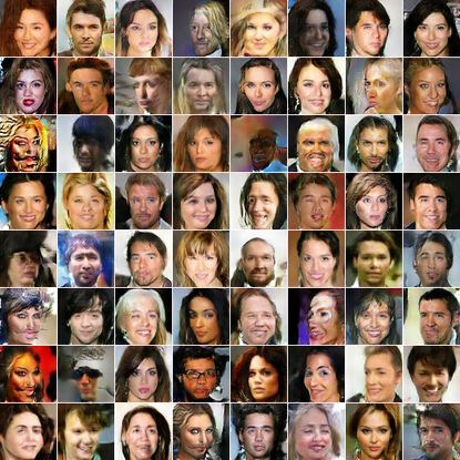
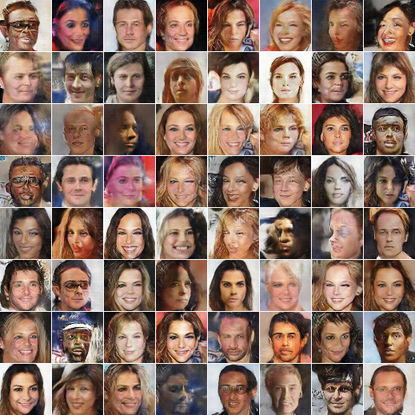
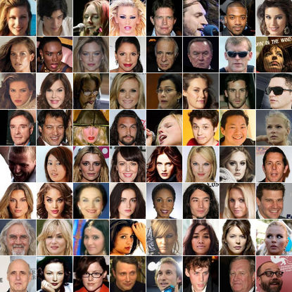
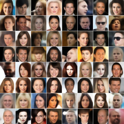
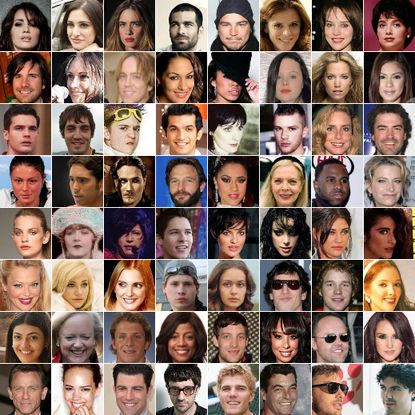
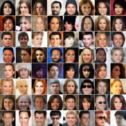
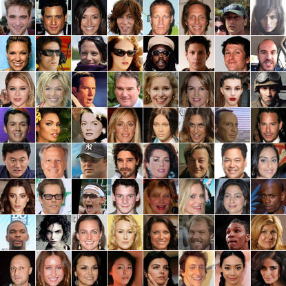
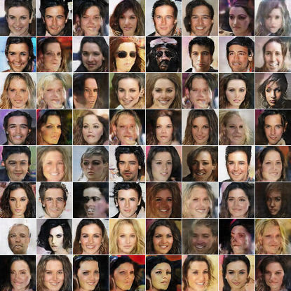
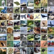
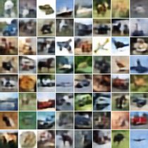
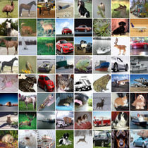
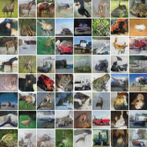
We show reconstructions obtained using VGH++ and VAEs for the CelebA dataset in Figure 25 and on CIFAR-10 in Figure 26.


Appendix M Model samples for real data experiments
