Tighter Variational Bounds are Not Necessarily Better

Abstract

We provide theoretical and empirical evidence that using tighter evidence lower bounds (elbos) can be detrimental to the process of learning an inference network by reducing the signal-to-noise ratio of the gradient estimator. Our results call into question common implicit assumptions that tighter elbos are better variational objectives for simultaneous model learning and inference amortization schemes. Based on our insights, we introduce three new algorithms: the partially importance weighted auto-encoder (piwae), the multiply importance weighted auto-encoder (miwae), and the combination importance weighted auto-encoder (ciwae), each of which includes the standard importance weighted auto-encoder (iwae) as a special case. We show that each can deliver improvements over iwae, even when performance is measured by the iwae target itself. Furthermore, our results suggest that piwae may be able to deliver simultaneous improvements in the training of both the inference and generative networks.

1 Introduction

Variational bounds provide tractable and state-of-the-art objectives for training deep generative models (Kingma & Welling, 2014; Rezende et al., 2014). Typically taking the form of a lower bound on the intractable model evidence, they provide surrogate targets that are more amenable to optimization. In general, this optimization requires the generation of approximate posterior samples during the model training and so a number of methods simultaneously learn an inference network alongside the target generative network.

As well as assisting the training process, this inference network is often also of direct interest itself. For example, variational bounds are often used to train auto-encoders (Bourlard & Kamp, 1988; Hinton & Zemel, 1994; Gregor et al., 2016; Chen et al., 2017), for which the inference network forms the encoder. Variational bounds are also used in amortized and traditional Bayesian inference contexts (Hoffman et al., 2013; Ranganath et al., 2014; Paige & Wood, 2016; Le et al., 2017), for which the generative model is fixed and the inference network is the primary target for the training.

The performance of variational approaches depends upon the choice of evidence lower bound (elbo) and the formulation of the inference network, with the two often intricately linked to one another; if the inference network formulation is not sufficiently expressive, this can have a knock-on effect on the generative network (Burda et al., 2016). In choosing the elbo, it is often implicitly assumed that using tighter elbos is universally beneficial, at least whenever this does not in turn lead to higher variance gradient estimates.

In this work we question this implicit assumption by demonstrating that, although using a tighter elbo is typically beneficial to gradient updates of the generative network, it can be detrimental to updates of the inference network. Remarkably, we find that it is possible to simultaneously tighten the bound, reduce the variance of the gradient updates, and arbitrarily deteriorate the training of the inference network.

Specifically, we present theoretical and empirical evidence that increasing the number of importance sampling particles, $K$, to tighten the bound in the importance-weighted auto-encoder (iwae) (Burda et al., 2016), degrades the signal-to-noise ratio (snr) of the gradient estimates for the inference network, inevitably deteriorating the overall learning process. In short, this behavior manifests because even though increasing $K$ decreases the standard deviation of the gradient estimates, it decreases the magnitude of the true gradient faster, such that the relative variance increases.

Our results suggest that it may be best to use distinct objectives for learning the generative and inference networks, or that when using the same target, it should take into account the needs of both networks. Namely, while tighter bounds are typically better for training the generative network, looser bounds are often preferable for training the inference network. Based on these insights, we introduce three new algorithms: the partially importance-weighted auto-encoder (piwae), the multiply importance-weighted auto-encoder (miwae), and the combination importance-weighted auto-encoder (ciwae). Each of these include iwae as a special case and are based on the same set of importance weights, but use these weights in different ways to ensure a higher SNR for the inference network.

We demonstrate that our new algorithms can produce inference networks more closely representing the true posterior than iwae, while matching the training of the generative network, or potentially even improving it in the case of piwae. Even when treating the iwae objective itself as the measure of performance, all our algorithms are able to demonstrate clear improvements over iwae.

2 Background and Notation

Let $x$ be an $\mathcal{X}$-valued random variable defined via a process involving an unobserved $\mathcal{Z}$-valued random variable $z$ with joint density $p_{\theta}(x,z)$. Direct maximum likelihood estimation of $\theta$ is generally intractable if $p_{\theta}(x,z)$ is a deep generative model due to the marginalization of $z$. A common strategy is to instead optimize a variational lower bound on $\log p_{\theta}(x)$, defined via an auxiliary inference model $q_{\phi}(z\lvert x)$:

$$\operatorname{\lx@glossaries@gls@link{acronym}{ELBO}{\leavevmode\textsc{elbo}}}_{\text{VAE}} (\theta,\phi,x)\coloneqq\int q_{\phi}(z\lvert x)\log\frac{p_{\theta}(x,z)}{q_{\phi}(z\lvert x)}\,\mathrm{d}z$$

$$=\log p_{\theta}(x)-\mathrm{KL}(q_{\phi}(z\lvert x)||p_{\theta}(z\lvert x)).$$ (1)

Typically, $q_{\phi}$ is parameterized by a neural network, for which the approach is known as the variational auto-encoder (vae) (Kingma & Welling, 2014; Rezende et al., 2014). Optimization is performed with stochastic gradient ascent (sga) using unbiased estimates of $\nabla_{\theta,\phi}\operatorname{\lx@glossaries@gls@link{acronym}{ELBO}{\leavevmode\textsc{elbo}}}_{\text{VAE}}(\theta,\phi,x)$. If $q_{\phi}$ is reparameterizable, then given a reparameterized sample $z\sim q_{\phi}(z\lvert x)$, the gradients $\nabla_{\theta,\phi}(\log p_{\theta}(x,z)-\log q_{\phi}(z\lvert x))$ can be used for the optimization.

The vae objective places a harsh penalty on mismatch between $q_{\phi}(z\lvert x)$ and $p_{\theta}(z\lvert x)$; optimizing jointly in $\theta,\phi$ can confound improvements in $\log p_{\theta}(x)$ with reductions in the KL (Turner & Sahani, 2011). Thus, research has looked to develop bounds that separate the tightness of the bound from the expressiveness of the class of $q_{\phi}$. For example, the iwae objectives (Burda et al., 2016), which we denote as $\operatorname{\lx@glossaries@gls@link{acronym}{ELBO}{\leavevmode\textsc{elbo}}}_{\text{IS}}(\theta,\phi,x)$, are a family of bounds defined by

$$Q_{\text{IS}}(z_{1:K}\lvert x) \coloneqq\prod\nolimits_{k=1}^{K}q_{\phi}(z_{k}\lvert x),$$

$$\hat{Z}_{\text{IS}}(z_{1:K},x) \coloneqq\frac{1}{K}\sum\nolimits_{k=1}^{K}\frac{p_{\theta}(x,z_{k})}{q_{\phi}(z_{k}\lvert x)},$$ (2)

$$\operatorname{\lx@glossaries@gls@link{acronym}{ELBO}{\leavevmode\textsc{elbo}}}_{\text{IS}}(\theta,\phi,x) \coloneqq\int Q_{\text{IS}}(z_{1:K}\lvert x)\log\hat{Z}_{\text{IS}}(z_{1:K},x)\,\mathrm{d}z_{1:K}$$

$\leq\log p_{\theta}(x)$. The iwae objectives generalize the vae objective ($K=1$ corresponds to the vae) and the bounds become strictly tighter as $K$ increases (Burda et al., 2016). When the family of $q_{\phi}$ contains the true posteriors, the global optimum parameters $\{\theta^{*},\phi^{*}\}$ are independent of $K$, see e.g. (Le et al., 2018). Nonetheless, except for the most trivial models, it is not usually the case that $q_{\phi}$ contains the true posteriors, and Burda et al. (2016) provide strong empirical evidence that setting $K>1$ leads to significant empirical gains over the vae in terms of learning the generative model.

Optimizing tighter bounds is usually empirically associated with better models $p_{\theta}$ in terms of marginal likelihood on held out data. Other related approaches extend this to sequential Monte Carlo (smc) (Maddison et al., 2017; Le et al., 2018; Naesseth et al., 2018) or change the lower bound that is optimized to reduce the bias (Li & Turner, 2016; Bamler et al., 2017). A second, unrelated, approach is to tighten the bound by improving the expressiveness of $q_{\phi}$ (Salimans et al., 2015; Tran et al., 2015; Rezende & Mohamed, 2015; Kingma et al., 2016; Maaløe et al., 2016; Ranganath et al., 2016). In this work, we focus on the former, algorithmic, approaches to tightening bounds.

3 Assessing the Signal-to-Noise Ratio of the Gradient Estimators

Because it is not feasible to analytically optimize any elbo in complex models, the effectiveness of any particular choice of elbo is linked to our ability to numerically solve the resulting optimization problem. This motivates us to examine the effect $K$ has on the variance and magnitude of the gradient estimates of iwae for the two networks. More generally, we study iwae gradient estimators constructed as the average of $M$ estimates, each built from $K$ independent particles. We present a result characterizing the asymptotic signal-to-noise ratio in $M$ and $K$. For the standard case of $M=1$, our result shows that the signal-to-noise ratio of the reparameterization gradients of the inference network for the iwae decreases with rate $O(1/\sqrt{K})$.

As estimating the $\operatorname{\lx@glossaries@gls@link{acronym}{ELBO}{\leavevmode\textsc{elbo}}}$ requires a Monte Carlo estimation of an expectation over $z$, we have two sample sizes to tune for the estimate: the number of samples $M$ used for Monte Carlo estimation of the elbo and the number of importance samples $K$ used in the bound construction. Here $M$ does not change the true value of $\nabla_{\theta,\phi}\operatorname{\lx@glossaries@gls@link{acronym}{ELBO}{\leavevmode\textsc{elbo}}}$, only our variance in estimating it, while changing $K$ changes the elbo itself, with larger $K$ leading to tighter bounds (Burda et al., 2016). Presuming that reparameterization is possible, we can express our gradient estimate in the general form

$$\Delta_{M,K}:= \frac{1}{M}\sum\nolimits_{m=1}^{M}\nabla_{\theta,\phi}\log\frac{1}{K}\sum\nolimits_{k=1}^{K}w_{m,k},$$ (3)

$$\text{where}\,\,w_{m,k} =\frac{p_{\theta}(z_{m,k},x)}{q_{\phi}(z_{m,k}\lvert x)}\,\,\text{and}\,\,z_{m,k}\overset{i.i.d.}{\sim}q_{\phi}(z_{m,k}\lvert x).$$

Thus, for a fixed budget of $T=MK$ samples, we have a family of estimators with the cases $K=1$ and $M=1$ corresponding respectively to the vae and iwae objectives. We will use ${\Delta}_{M,K}\left(\theta\right)$ to refer to gradient estimates with respect to $\theta$ and ${\Delta}_{M,K}\left(\phi\right)$ for those with respect to $\phi$.

Variance is not always a good barometer for the effectiveness of a gradient estimation scheme; estimators with small expected values need proportionally smaller variances to be estimated accurately. In the case of iwae, when changes in $K$ simultaneously affect both the variance and expected value, the quality of the estimator for learning can actually worsen as the variance decreases. To see why, consider the marginal likelihood estimates $\hat{Z}_{m,K}=\sum_{k=1}^{K}w_{m,k}$. Because these become exact (and thus independent of the proposal) as $K\to\infty$, it must be the case that $\lim_{K\rightarrow\infty}{\Delta}_{M,K}(\phi)=0$. Thus as $K$ becomes large, the expected value of the gradient must decrease along with its variance, such that the variance relative to the problem scaling need not actually improve.

To investigate this formally, we introduce the signal-to-noise-ratio (snr), defining it to be the absolute value of the expected estimate scaled by its standard deviation:

$$\operatorname{\lx@glossaries@gls@link{acronym}{SNR}{\leavevmode\textsc{snr}}}_{M,K}(\theta) =\left|\mathbb{E}\left[\Delta_{M,K}(\theta)\right]/\sigma\left[\Delta_{M,K}(\theta)\right]\right|$$ (4)

where $\sigma[\cdot]$ denotes the standard deviation of a random variable. The snr is defined separately on each dimension of the parameter vector and similarly for $\operatorname{\lx@glossaries@gls@link{acronym}{SNR}{\leavevmode\textsc{snr}}}_{M,K}(\phi)$. It provides a measure of the relative accuracy of the gradient estimates. Though a high snr does not always indicate a good sga scheme (as the target objective itself might be poorly chosen), a low snr is always problematic as it indicates that the gradient estimates are dominated by noise: if $\operatorname{\lx@glossaries@gls@link{acronym}{SNR}{\leavevmode\textsc{snr}}}\to 0$ then the estimates become completely random. We are now ready to state our main theoretical result: $\operatorname{\lx@glossaries@gls@link{acronym}{SNR}{\leavevmode\textsc{snr}}}_{M,K}(\theta)=O(\sqrt{MK})$ and $\operatorname{\lx@glossaries@gls@link{acronym}{SNR}{\leavevmode\textsc{snr}}}_{M,K}(\phi)=O(\sqrt{M/K})$.

Theorem 1.

Assume that when $M=K=1$, the expected gradients; the variances of the gradients; and the first four moments of $w_{1,1}$, $\nabla_{\theta}w_{1,1}$, and $\nabla_{\phi}w_{1,1}$ are all finite and the variances are also non-zero. Then the signal-to-noise ratios of the gradient estimates converge at the following rates

$$\operatorname{\lx@glossaries@gls@link{acronym}{SNR}{\leavevmode\textsc{snr}}}_{M,K}(\theta)=$$ (5)

$$\sqrt{M}\left|\frac{\sqrt{K}\;\nabla_{\theta}Z-\frac{1}{2Z\sqrt{K}}\nabla_{\theta}\left(\frac{\textnormal{Var}\left[w_{1,1}\right]}{Z^{2}}\right)+O\left(\frac{1}{K^{3/2}}\right)}{\sqrt{\mathbb{E}\left[w_{1,1}^{2}\left(\nabla_{\theta}\log w_{1,1}-\nabla_{\theta}\log Z\right)^{2}\right]}+O\left(\frac{1}{K}\right)}\right|$$

$$\operatorname{\lx@glossaries@gls@link{acronym}{SNR}{\leavevmode\textsc{snr}}}_{M,K}(\phi)=\sqrt{M}\left|\frac{\nabla_{\phi}\textnormal{Var}\left[w_{1,1}\right]+O\left(\frac{1}{K}\right)}{2Z\sqrt{K}\;\sigma\left[\nabla_{\phi}w_{1,1}\right]+O\left(\frac{1}{\sqrt{K}}\right)}\right|$$ (6)

where $Z:=p_{\theta}(x)$ is the true marginal likelihood.

Proof.

We give an intuitive demonstration of the result here and provide a formal proof in Appendix A. The effect of $M$ on the snr follows from using the law of large numbers on the random variable $\nabla_{\theta,\phi}\log\hat{Z}_{m,K}$. Namely, the overall expectation is independent of $M$ and the variance reduces at a rate $O(1/M)$. The effect of $K$ is more complicated but is perhaps most easily seen by noting that (Burda et al., 2016)

$$\nabla_{\theta,\phi}\log\hat{Z}_{m,K}=\sum_{k=1}^{K}\frac{w_{m,k}}{\sum_{\ell=1}^{K}w_{m,k}}\nabla_{\theta,\phi}\log\left(w_{m,k}\right),$$

such that $\nabla_{\theta,\phi}\log\hat{Z}_{m,K}$ can be interpreted as a self-normalized importance sampling estimate. We can, therefore, invoke the known result (see e.g. Hesterberg (1988)) that the bias of a self-normalized importance sampler converges at a rate $O(1/K)$ and the standard deviation at a rate $O(1/\sqrt{K})$. We thus see that the snr converges at a rate $O((1/K)/(1/\sqrt{K}))=O(1/\sqrt{K})$ if the asymptotic gradient is $0$ and $O((1)/(1/\sqrt{K}))=O(\sqrt{K})$ otherwise, giving the convergence rates in the $\phi$ and $\theta$ cases respectively. ∎

The implication of these rates is that increasing $M$ is monotonically beneficial to the snr for both $\theta$ and $\phi$, but that increasing $K$ is beneficial to the former and detrimental to the latter. We emphasize that this means the snr for the iwae inference network gets worse as we increase $K$: this is not just an opportunity cost from the fact that we could have increased $M$ instead, increasing the total number of samples used in the estimator actually worsens the snr!

3.1 Asymptotic Direction

An important point of note is that the dependence of the true inference network gradients becomes independent of $K$ as $K$ becomes large. Namely, because we have as an intermediary result from deriving the snrs that

$$\mathbb{E}\left[\Delta_{M,K}(\phi)\right]=-\frac{\nabla_{\phi}\text{Var}\left[w_{1,1}\right]}{2KZ^{2}}+O\left(\frac{1}{K^{2}}\right),$$ (7)

we see that expected gradient points in the direction of $-\nabla_{\phi}\text{Var}\left[w_{1,1}\right]$ as $K\to\infty$. This direction is rather interesting: it implies that as $K\to\infty$, the optimal $\phi$ is that which minimizes the variance of the weights. This is well known to be the optimal importance sampling distribution in terms of estimating the marginal likelihood (Owen, 2013). Given that the role of the inference network during training is to estimate the marginal likelihood, this is thus arguably exactly what we want to optimize for. As such, this result, which complements those of (Cremer et al., 2017), suggests that increasing $K$ provides a preferable target in terms of the direction of the true inference network gradients. We thus see that there is a trade-off with the fact that increasing $K$ also diminishes the snr, reducing the estimates to pure noise if $K$ is set too high. In the absence of other factors, there may thus be a “sweet-spot” for setting $K$.

(a) iwae inference network gradient estimates

(b) iwae generative network gradient estimates

Figure 1: Histograms of gradient estimates $\Delta_{M,K}$ for the generative network and the inference network using the iwae ($M=1$) objective with different values of $K$.

3.2 Multiple Data Points

Typically when training deep generative models, one does not optimize a single elbo but instead its average over multiple data points, i.e.

$$\mathcal{J}(\theta,\phi) :=\frac{1}{N}\sum\nolimits_{n=1}^{N}\operatorname{\lx@glossaries@gls@link{acronym}{ELBO}{\leavevmode\textsc{elbo}}}_{\text{IS}}(\theta,\phi,x^{(n)}).$$ (8)

Our results extend to this setting because the $z$ are drawn independently for each $x^{(n)}$, so

$$\mathbb{E}\left[\frac{1}{N}\sum\nolimits_{n=1}^{N}\Delta_{M,K}^{(n)}\right] =\frac{1}{N}\sum\nolimits_{n=1}^{N}\mathbb{E}\left[\Delta_{M,K}^{(n)}\right],$$ (9)

$$\text{Var}\left[\frac{1}{N}\sum\nolimits_{n=1}^{N}\Delta_{M,K}^{(n)}\right] =\frac{1}{N^{2}}\sum\nolimits_{n=1}^{N}\text{Var}\left[\Delta_{M,K}^{(n)}\right].$$ (10)

We thus also see that if we are using mini-batches such that $N$ is a chosen parameter and the $x^{(n)}$ are drawn from the empirical data distribution, then the snrs of $\bar{\Delta}_{N,M,K}:=\frac{1}{N}\sum_{n=1}^{N}\Delta_{M,K}^{(n)}$ scales as $\sqrt{N}$, i.e. $\operatorname{\lx@glossaries@gls@link{acronym}{SNR}{\leavevmode\textsc{snr}}}_{N,M,K}(\theta)=O(\sqrt{NMK})$ and $\operatorname{\lx@glossaries@gls@link{acronym}{SNR}{\leavevmode\textsc{snr}}}_{N,M,K}(\phi)=O(\sqrt{NM/K})$. Therefore increasing $N$ has the same ubiquitous benefit as increasing $M$. In the rest of the paper, we will implicitly be considering the snrs for $\bar{\Delta}_{N,M,K}$, but will omit the dependency on $N$ to simplify the notation.

4 Empirical Confirmation

Our convergence results hold exactly in relation to $M$ (and $N$) but are only asymptotic in $K$ due to the higher order terms. Therefore their applicability should be viewed with a healthy degree of skepticism in the small $K$ regime. With this in mind, we now present empirical support for our theoretical results and test how well they hold in the small $K$ regime using a simple Gaussian model, for which we can analytically calculate the ground truth.

Consider a family of generative models with $\mathbb{R}^{D}$–valued latent variables $z$ and observed variables $x$:

$$z\sim\mathcal{N}(z;\mu,I), x\lvert z\sim\mathcal{N}(x;z,I),$$ (11)

which is parameterized by $\theta:=\mu$. Let the inference network be parameterized by $\phi=(A,b),\;A\in\mathbb{R}^{D\times D},\;b\in\mathbb{R}^{D}$ where $q_{\phi}(z\lvert x)=\mathcal{N}(z;Ax+b,\frac{2}{3}I)$. Given a dataset $(x^{(n)})_{n=1}^{N}$, we can analytically calculate the optimum of our target $\mathcal{J}(\theta,\phi)$ as explained in Appendix B, giving $\theta^{*}:=\mu^{*}=\frac{1}{N}\sum_{n=1}^{N}x^{(n)}$ and $\phi^{*}:=(A^{*},b^{*})$, where $A^{*}=I/2$ and $b^{*}=\mu^{*}/2$. Though this will not be the case in general, for this particular problem, the optimal proposal is independent of $K$. However, the expected gradients for the inference network still change with $K$.

(a) Convergence of snr for inference network

(b) Convergence of snr for generative network

Figure 2: Convergence of signal-to-noise ratios of gradient estimates with increasing $M$ and $K$. Different lines correspond to different dimensions of the parameter vectors. Shown in blue is the iwae where we keep $M=1$ fixed and increase $K$. Shown in red is the vae where $K=1$ is fixed and we increase $M$. The black and green dashed lines show the expected convergence rates from our theoretical results, representing gradients of $1/2$ and $-1/2$ respectively.

To conduct our investigation, we randomly generated a synthetic dataset from the model with $D=20$ dimensions, $N=1024$ data points, and a true model parameter value $\mu_{\text{true}}$ that was itself randomly generated from a unit Gaussian, i.e. $\mu_{\text{true}}\sim\mathcal{N}(\mu_{\text{true}};0,I)$. We then considered the gradient at a random point in the parameter space close to optimum (we also consider a point far from the optimum in Appendix C.3). Namely each dimension of each parameter was randomly offset from its optimum value using a zero-mean Gaussian with standard deviation $0.01$. We then calculated empirical estimates of the elbo gradients for iwae, where $M=1$ is held fixed and we increase $K$, and for vae, where $K=1$ is held fixed and we increase $M$. In all cases we calculated $10^{4}$ such estimates and used these samples to provide empirical estimates for, amongst other things, the mean and standard deviation of the estimator, and thereby an empirical estimate for the snr.

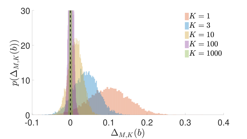
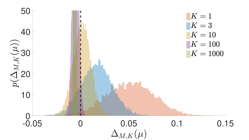
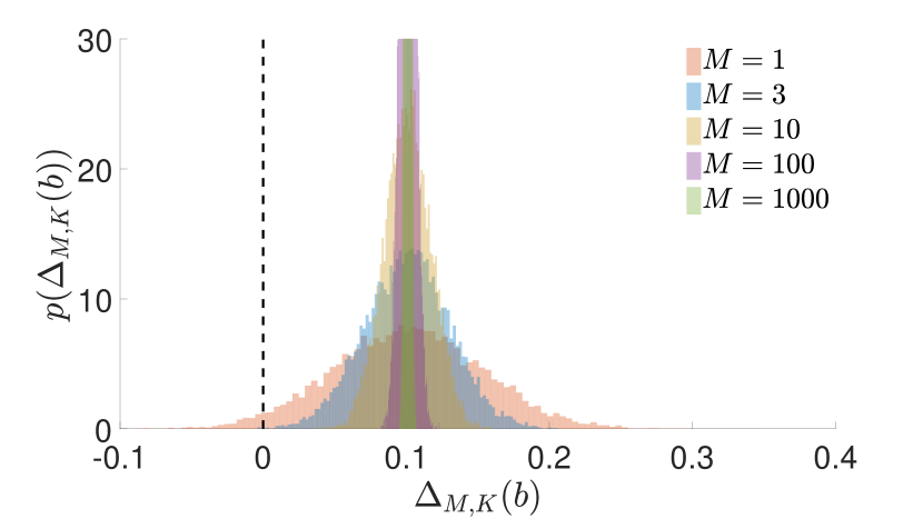
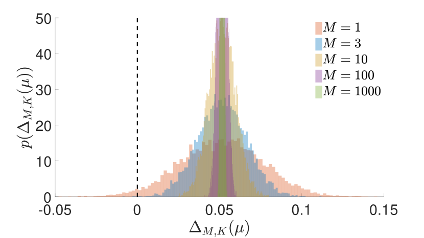
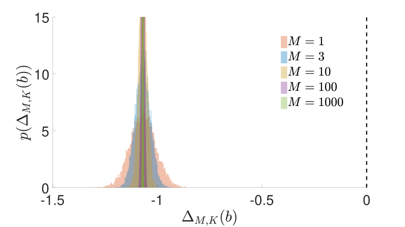
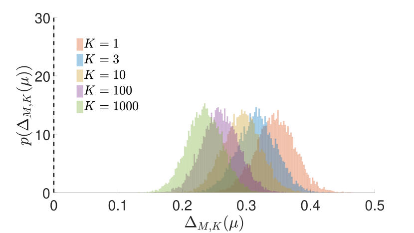
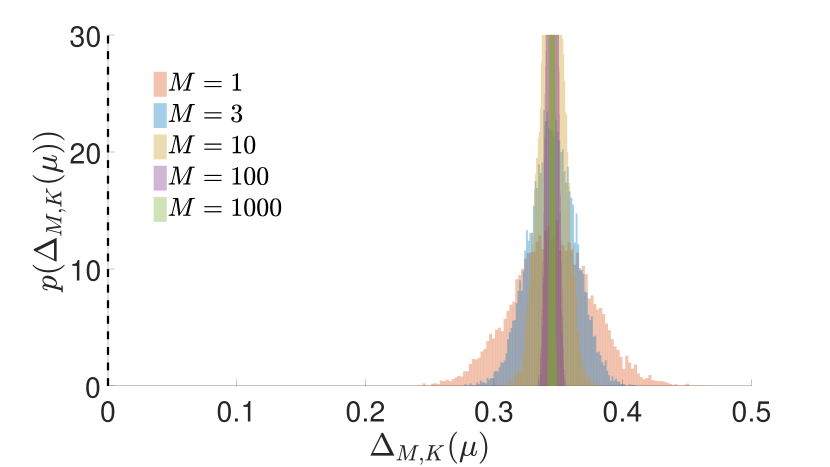
We start by examining the qualitative behavior of the different gradient estimators as $K$ increases as shown in Figure 1. This shows histograms of the iwae gradient estimators for a single parameter of the inference network (left) and generative network (right). We first see in Figure 1(a) that as $K$ increases, both the magnitude and the standard deviation of the estimator decrease for the inference network, with the former decreasing faster. This matches the qualitative behavior of our theoretical result, with the snr ratio diminishing as $K$ increases. In particular, the probability that the gradient is positive or negative becomes roughly equal for larger values of $K$, meaning the optimizer is equally likely to increase as decrease the inference network parameters at the next iteration. By contrast, for the generative network, iwae converges towards a non-zero gradient, such that, even though the snr initially decreases with $K$, it then rises again, with a very clear gradient signal for $K=1000$.

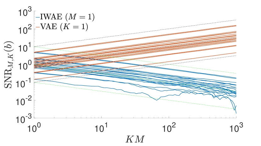
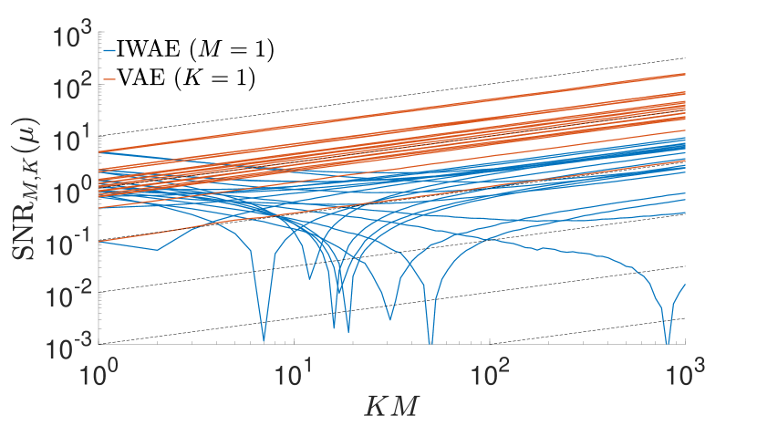
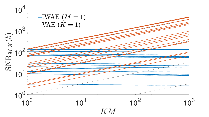
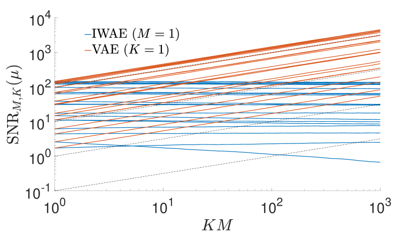
To provide a more rigorous analysis, we next directly examine the convergence of the snr. Figure 2 shows the convergence of the estimators with increasing $M$ and $K$. The observed rates for the inference network (Figure 2(a)) correspond to our theoretical results, with the suggested rates observed all the way back to $K=M=1$. As expected, we see that as $M$ increases, so does $\operatorname{\lx@glossaries@gls@link{acronym}{SNR}{\leavevmode\textsc{snr}}}_{M,K}(b)$, but as $K$ increases, $\operatorname{\lx@glossaries@gls@link{acronym}{SNR}{\leavevmode\textsc{snr}}}_{M,K}(b)$ reduces.

In Figure 2(b), we see that the theoretical convergence for $\operatorname{\lx@glossaries@gls@link{acronym}{SNR}{\leavevmode\textsc{snr}}}_{M,K}(\mu)$ is again observed exactly for variations in $M$, but a more unusual behavior is seen for variations in $K$, where the snr initially decreases before starting to increase again for large enough $K$, eventually exhibiting behavior consistent with the theoretical result for large enough $K$. The driving factor for this is that here $\mathbb{E}[\Delta_{M,\infty}(\mu)]$ has a smaller magnitude than (and opposite sign to) $\mathbb{E}[\Delta_{M,1}(\mu)]$ (see Figure 1(b)). If we think of the estimators for all values of $K$ as biased estimates for $\mathbb{E}[\Delta_{M,\infty}(\mu)]$, we see from our theoretical results that this bias decreases faster than the standard deviation. Consequently, while the magnitude of this bias remains large compared to $\mathbb{E}[\Delta_{M,\infty}(\mu)]$, it is the predominant component in the true gradient and we see similar snr behavior as in the inference network.

Note that this does not mean that the estimates are getting worse for the generative network. As we increase $K$ our bound is getting tighter and our estimates closer to the true gradient for the target that we actually want to optimize $\nabla_{\mu}\log Z$. See Appendix C.2 for more details. As we previously discussed, it is also the case that increasing $K$ could be beneficial for the inference network even if it reduces the snr by improving the direction of the expected gradient. However, as we will now show, the snr is, for this problem, the dominant effect for the inference network.

(a) Convergence of dsnr for inference network

(b) Convergence of dsnr for generative network

Figure 3: Convergence of the directional snr of gradients estimates with increasing $M$ and $K$. The solid lines show the estimated dsnr and the shaded regions the interquartile range of the individual ratios. Also shown for reference is the dsnr for a randomly generated vector where each component is drawn from a unit Gaussian.

(a) Convergence of dsnr for inference network

(b) Convergence of dsnr for generative network

Figure 4: Convergence of the dsnr when the target gradient is taken as $u=\mathbb{E}\left[\Delta_{1,1000}\right]$. Conventions as per Figure 3.

4.1 Directional Signal-to-Noise Ratio

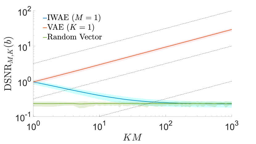
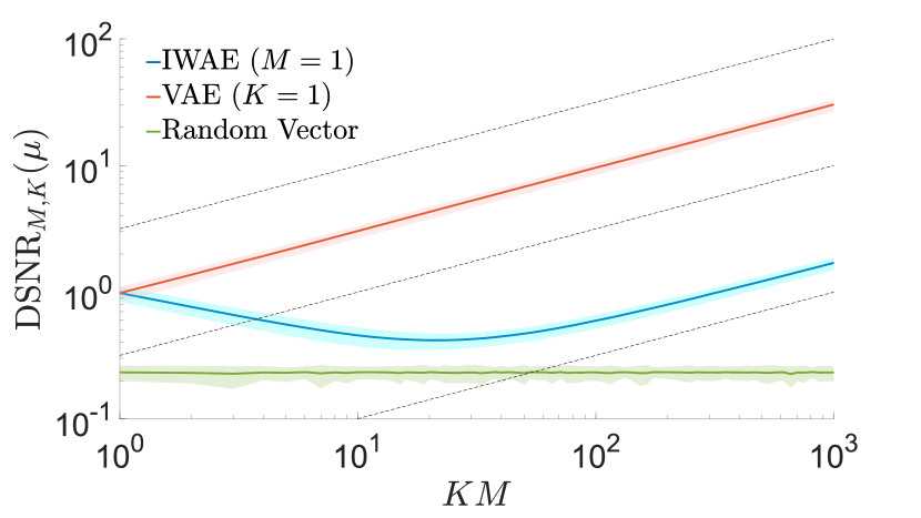
As a reassurance that our chosen definition of the snr is appropriate for the problem at hand and to examine the effect of multiple dimensions explicitly, we now also consider an alternative definition of the snr that is similar (though distinct) to that used in (Roberts & Tedrake, 2009). We refer to this as the “directional” snr (dsnr). At a high-level, we define the dsnr by splitting each gradient estimate into two component vectors, one parallel to the true gradient and one perpendicular, then taking the expectation of ratio of their magnitudes. More precisely, we define $u=\mathbb{E}\left[\Delta_{M,K}\right]/\lVert\mathbb{E}\left[\Delta_{M,K}\right]\rVert_{2}$ as being the true normalized gradient direction and then the dsnr as

$$\textsc{dsnr}_{M,K}= \,\,\mathbb{E}\left[\frac{\lVert\Delta_{\|}\rVert_{2}}{\lVert\Delta_{\bot}\rVert_{2}}\right]\quad\text{where}$$ (12)

$$\Delta_{\|}=\left(\Delta_{M,K}^{T}u\right)u \quad\text{and}\quad\Delta_{\bot}=\Delta_{M,K}-\Delta_{\|}.$$

The dsnr thus provides a measure of the expected proportion of the gradient that will point in the true direction. For perfect estimates of the gradients, then $\textsc{dsnr}\to\infty$, but unlike the snr, arbitrarily bad estimates do not have $\textsc{dsnr}=0$ because even random vectors will have a component of their gradient in the true direction.

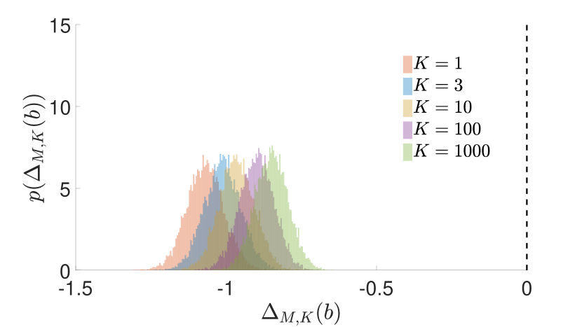
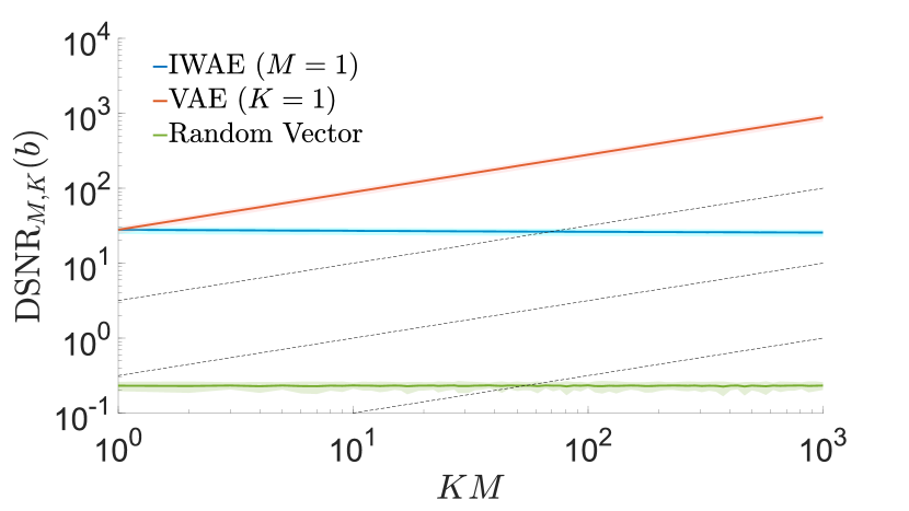
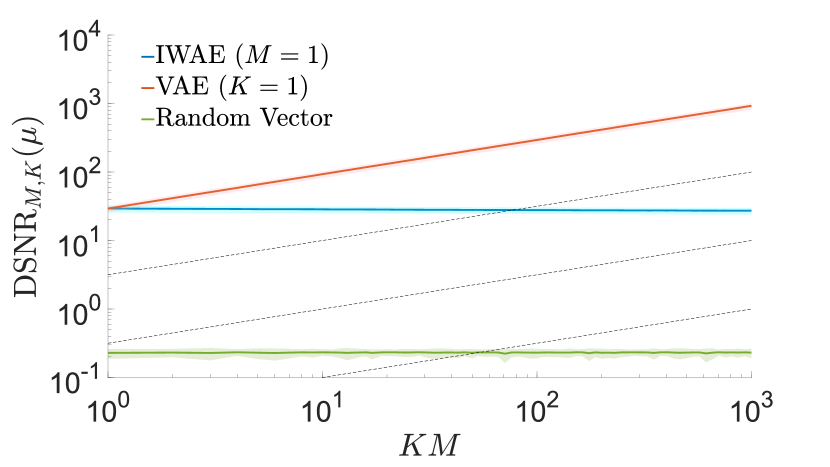
The convergence of the dsnr is shown in Figure 3, for which the true normalized gradient $u$ has been estimated empirically, noting that this varies with $K$. We see a similar qualitative behavior to the snr, with the gradients of iwae for the inference network degrading to having the same directional accuracy as drawing a random vector. Interestingly, the dsnr seems to be following the same asymptotic convergence behavior as the snr for both networks in $M$ (as shown by the dashed lines), even though we have no theoretical result to suggest this should occur.

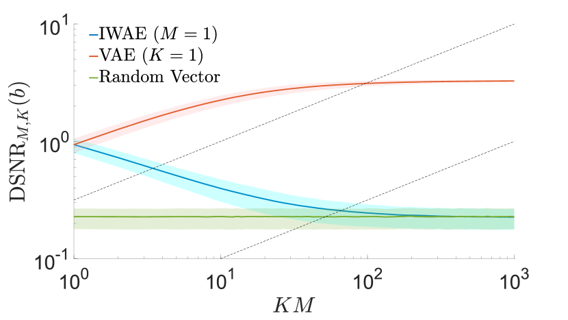
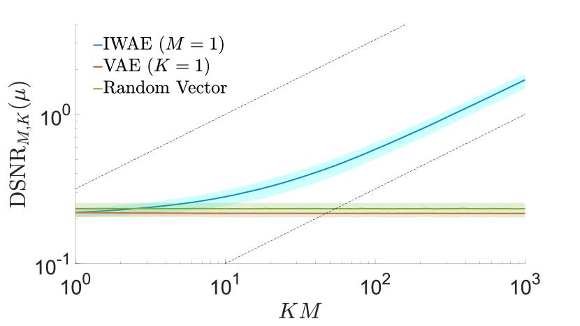
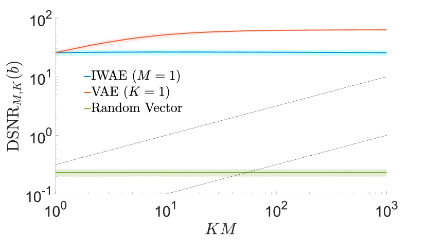
As our theoretical results suggest that the direction of the true gradients correspond to targeting an improved objective as $K$ increases, we now examine whether this or the changes in the snr is the dominant effect. To this end, we repeat our calculations for the dsnr but take $u$ as the target direction of the gradient for $K=1000$. This provides a measure of how varying $M$ and $K$ affects the quality of the gradient directions as biased estimators for $\mathbb{E}\left[\Delta_{1,1000}\right]/\lVert\mathbb{E}\left[\Delta_{1,1000}\right]\rVert_{2}$. As shown in Figure 4, increasing $K$ is still detrimental for the inference network by this metric, even though it brings the expected gradient estimate closer to the target gradient. By contrast, increasing $K$ is now monotonically beneficial for the generative network. Increasing $M$ leads to initial improvements for the inference network before plateauing due to the bias of the estimator. For the generative network, increasing $M$ has little impact, with the bias being the dominant factor throughout. Though this metric is not an absolute measure of performance of the sga scheme, e.g. because high bias may be more detrimental than high variance, it is nonetheless a powerful result in suggesting that increasing $K$ can be detrimental to learning the inference network.

5 New Estimators

Based on our theoretical results, we now introduce three new algorithms that address the issue of diminishing snr for the inference network. Our first, miwae, is exactly equivalent to the general formulation given in (3), the distinction from previous approaches coming from the fact that it takes both $M>1$ and $K>1$. The motivation for this is that because our inference network snr increases as $O(\sqrt{M/K})$, we should be able to mitigate the issues increasing $K$ has on the snr by also increasing $M$. For fairness, we will keep our overall budget $T=MK$ fixed, but we will show that given this budget, the optimal value for $M$ is often not $1$. In practice, we expect that it will often be beneficial to increase the mini-batch size $N$ rather than $M$ for miwae; as we showed in Section 3.2 this has the same effect on the snr. Nonetheless, miwae forms an interesting reference method for testing our theoretical results and, as we will show, it can offer improvements over iwae for a given $N$.

Our second algorithm, ciwae uses a convex combination of the iwae and vae bounds, namely

$$\operatorname{\lx@glossaries@gls@link{acronym}{ELBO}{\leavevmode\textsc{elbo}}}_{\text{CIWAE}}=\beta\operatorname{\lx@glossaries@gls@link{acronym}{ELBO}{\leavevmode\textsc{elbo}}}_{\text{VAE}}+(1-\beta)\operatorname{\lx@glossaries@gls@link{acronym}{ELBO}{\leavevmode\textsc{elbo}}}_{\text{IWAE}}$$ (13)

where $\beta\in[0,1]$ is a combination parameter. It is trivial to see that $\operatorname{\lx@glossaries@gls@link{acronym}{ELBO}{\leavevmode\textsc{elbo}}}_{\text{CIWAE}}$ is a lower bound on the log marginal that is tighter than the vae bound but looser than the iwae bound. We then employ the following estimator

$$\Delta_{K,\beta}^{\text{C}}=$$ (14)

$$\nabla_{\theta,\phi} \left(\beta\frac{1}{K}\sum_{k=1}^{K}\log w_{k}+(1-\beta)\log\left(\frac{1}{K}\sum_{k=1}^{K}w_{k}\right)\right)$$

where we use the same $w_{k}$ for both terms. The motivation for ciwae is that, if we set $\beta$ to a relatively small value, the objective will behave mostly like iwae, except when the expected iwae gradient becomes very small. When this happens, the vae component should “take-over” and alleviate SNR issues: the asymptotic SNR of $\Delta_{K,\beta}^{\text{C}}$ for $\phi$ is $O(\sqrt{MK})$ because the vae component has non-zero expectation in the limit $K\rightarrow\infty$.

Our results suggest that what is good for the generative network, in terms of setting $K$, is often detrimental for the inference network. It is therefore natural to question whether it is sensible to always use the same target for both the inference and generative networks. Motivated by this, our third method, piwae, uses the iwae target when training the generative network, but the miwae target for training the inference network. We thus have

$$\Delta_{K,\beta}^{\text{C}}(\theta) =\nabla_{\theta}\log\frac{1}{K}\sum\nolimits_{k=1}^{K}w_{k}$$ (15a)

$$\Delta_{M,K,\beta}^{\text{C}}(\phi) =\frac{1}{M}\sum\nolimits_{m=1}^{M}\nabla_{\phi}\log\frac{1}{L}\sum\nolimits_{\ell=1}^{L}w_{m,\ell}$$ (15b)

where we will generally set $K=ML$ so that the same weights can be used for both gradients.

(a) IWAE₆₄

(b) $\log\hat{p}(x)$

(c) $-\mathrm{KL}(Q_{\phi}(z\lvert x)||P_{\theta}(z\lvert x))$

Figure 5: Convergence of evaluation metrics on the test set with increased training time. All lines show mean $\pm$ standard deviation over 4 runs with different random initializations. Larger values are preferable for each plot.

(a) Comparing miwae and iwae

(b) Comparing ciwae and iwae

(c) Comparing piwae and iwae

Figure 6: Test set performance of miwae, ciwae, and piwae relative to iwae in terms of the iwae-64 (top), $\log\hat{p}(x)$ (middle), and $-\mathrm{KL}(Q_{\phi}(z\lvert x)||P_{\theta}(z\lvert x))$ (bottom) metrics. All dots are the difference in the metric to that of iwae. Dotted line is the iwae baseline. Note that in all cases, the far left of the plot correspond to settings equivalent to the iwae.

Table 1: Mean final test set performance $\pm$ standard deviation over $4$ runs. Numbers in brackets in indicate $(M,K)$. The best result is shown in red, while bold results are not statistically significant to best result at the 5% level of a Welch’s t-test.

Metric	iwae	piwae $(4,16)$	piwae $(8,8)$	miwae $(4,16)$	miwae $(8,8)$	ciwae $\beta=0.05$	ciwae $\beta=0.5$	vae
iwae-$64$	–$86.11\pm 0.10$	–$\mathbf{85.68\pm 0.06}$	–$\mathbf{85.74\pm 0.07}$	–$\mathbf{85.60\pm 0.07}$	–$\mathbf{85.69\pm 0.04}$	–$85.91\pm 0.11$	–$86.08\pm 0.08$	–$86.69\pm 0.08$
$\log\hat{p}(x)$	–$\mathbf{84.52\pm 0.02}$	–$\mathbf{84.40\pm 0.17}$	–$\mathbf{84.46\pm 0.06}$	–$\mathbf{84.56\pm 0.05}$	–$84.97\pm 0.10$	–$\mathbf{84.57\pm 0.09}$	–$85.24\pm 0.08$	–$86.21\pm 0.19$
$-\mathrm{KL}(Q||P)$	–$1.59\pm 0.10$	–$1.27\pm 0.18$	–$1.28\pm 0.09$	–$\mathbf{1.04\pm 0.08}$	–$\mathbf{0.72\pm 0.11}$	–$1.34\pm 0.14$	–$\mathbf{0.84\pm 0.11}$	–$\mathbf{0.47\pm 0.20}$

5.1 Experiments

We now use our new estimators to train deep generative models for the MNIST digits dataset (LeCun et al., 1998). For this, we duplicated the architecture and training schedule outlined in Burda et al. (2016). In particular, all networks were trained and evaluated using their stochastic binarization. For all methods we set a budget of $T=64$ weights in the target estimate for each datapoint in the minibatch.

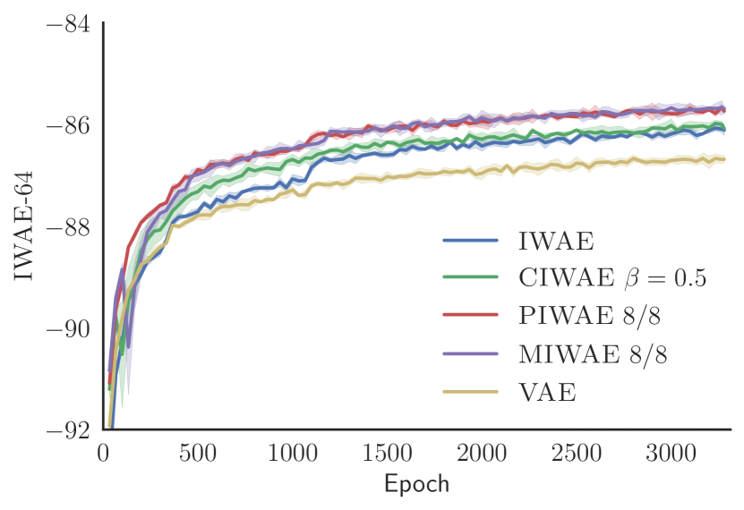
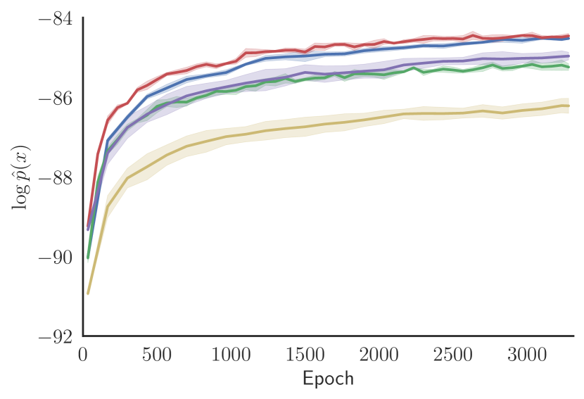
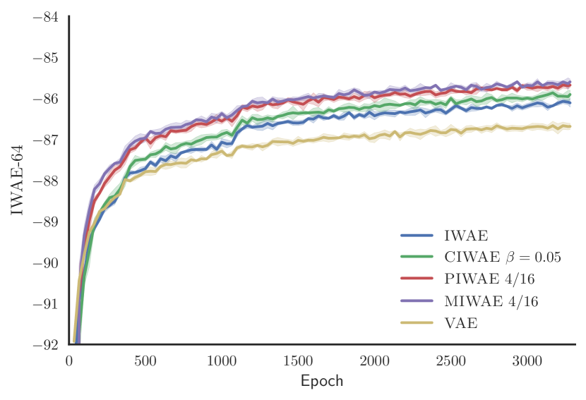
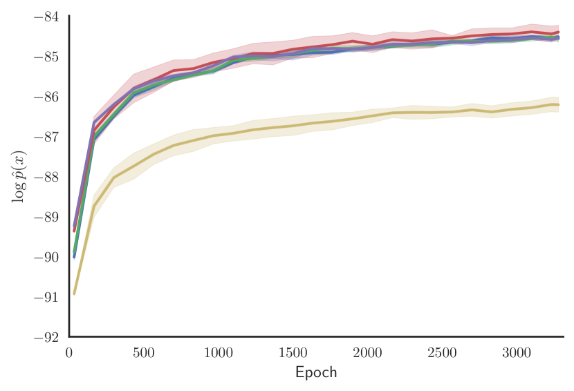
To assess different aspects of the training performance, we consider three different metrics: $\operatorname{\lx@glossaries@gls@link{acronym}{ELBO}{\leavevmode\textsc{elbo}}}_{\text{IWAE}}$ with $K=64$, $\operatorname{\lx@glossaries@gls@link{acronym}{ELBO}{\leavevmode\textsc{elbo}}}_{\text{IWAE}}$ with $K=5000$, and the latter of these minus the former. All reported metrics are evaluated on the test data.

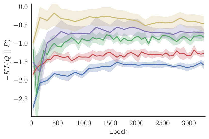
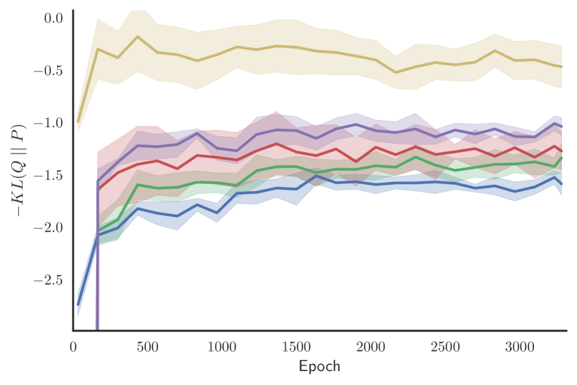
The motivation for the $\operatorname{\lx@glossaries@gls@link{acronym}{ELBO}{\leavevmode\textsc{elbo}}}_{\text{IWAE}}$ with $K=64$ metric, denoted as iwae-64, is that this is the target used for training the iwae and so if another method does better on this metric than the iwae, this is a clear indicator that snr issues of the iwae estimator have degraded its performance. In fact, this would demonstrate that, from a practical perspective, using the iwae estimator is sub-optimal, even if our explicit aim is to optimize the iwae bound. The second metric, $\operatorname{\lx@glossaries@gls@link{acronym}{ELBO}{\leavevmode\textsc{elbo}}}_{\text{IWAE}}$ with $K=5000$, denoted $\log\hat{p}(x)$, is used as a surrogate for estimating the log marginal likelihood and thus provides an indicator for fidelity of the learned generative model. The third metric is an estimator for the divergence implicitly targeted by the iwae. Namely, as shown by Le et al. (2018), the $\operatorname{\lx@glossaries@gls@link{acronym}{ELBO}{\leavevmode\textsc{elbo}}}_{\text{IWAE}}$ can be interpreted as

$$\operatorname{\lx@glossaries@gls@link{acronym}{ELBO}{\leavevmode\textsc{elbo}}}_{\text{IWAE}}=\log p_{\theta}(x)-\mathrm{KL}(Q_{\phi}(z\lvert x)||P_{\theta}(z\lvert x))$$ (16)

$$\text{where}\quad Q_{\phi}(z\lvert x):=\prod\nolimits_{k=1}^{K}q_{\phi}(z_{k}\lvert x),\quad\text{and}$$ (17)

$$P_{\theta}(z\lvert x):=\frac{1}{K}\sum\nolimits_{k=1}^{K}\frac{\prod_{\ell=1}^{K}q_{\phi}(z_{\ell}\lvert x)}{q_{\phi}(z_{k}\lvert x)}p_{\theta}(z_{k}\lvert x).$$ (18)

Thus we can estimate $\mathrm{KL}(Q_{\phi}(z\lvert x)||P_{\theta}(z\lvert x))$ using $\log\hat{p}(x)-{\text{IWAE-64}}$, to provide a metric for divergence between the inference network and the proposal network. We use this instead of $\mathrm{KL}(q_{\phi}(z\lvert x)||p_{\theta}(z\lvert x))$ because the latter can be deceptive metric for the inference network fidelity. For example, it tends to prefer $q_{\phi}(z\lvert x)$ that cover only one of the posterior modes, rather than encompassing all of them. As we showed in Section 3.1, the implied target of the true gradients for the inference network improves as $K$ increases and so $\mathrm{KL}(Q_{\phi}(z\lvert x)||P_{\theta}(z\lvert x))$ should be a more reliable metric of inference network performance.

Figure 5 shows the convergence of these metrics for each algorithm. Here we have considered the middle value for each of the parameters, namely $K=M=8$ for piwae and miwae, and $\beta=0.5$ for ciwae. We see that piwae and miwae both comfortably outperformed, and ciwae slightly outperformed, iwae in terms of iwae-64 metric, despite iwae being directly trained on this target. In terms of $\log\hat{p}(x)$, piwae gave the best performance, followed by iwae. For the KL, we see that the vae performed best followed by miwae, with iwae performing the worst. We note here that the KL is not an exact measure of the inference network performance as it also depends on the generative model. As such, the apparent superior performance of the vae may be because it produces a simpler model, as per the observations of Burda et al. (2016), which in turn is easier to learn an inference network for. Critically though, piwae improves this metric whilst also improving generative network performance, such that this reasoning no longer applies. Similar behavior is observed for miwae and ciwae for different parameter settings (see Appendix D).

Figure 7: Violin plots of ESS estimates for each image of MNIST, normalized by the number of samples drawn. A violin plot uses a kernel density plot on each side – thicker means more MNIST images whose $q_{\phi}$ achieves that ESS.

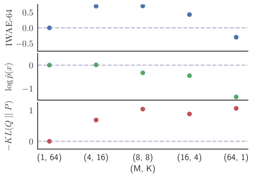
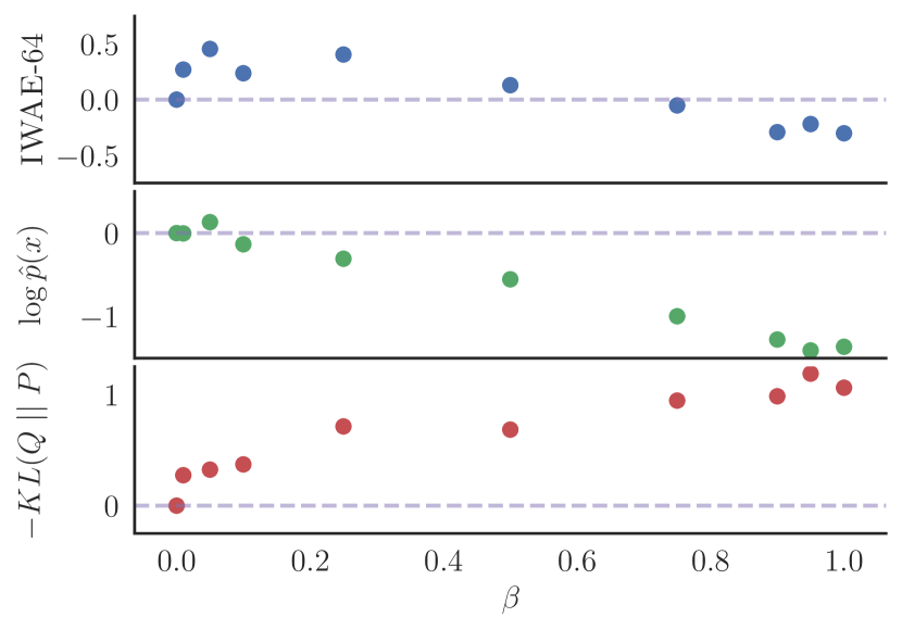
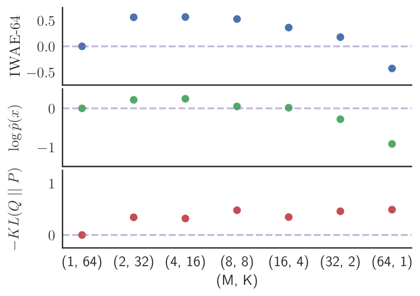
We next considered tuning the parameters for each of our algorithms as shown in Figure 6, for which we look at the final metric values after training. Table 1 further summarizes the performance for certain selected parameter settings. For miwae we see that as we increase $M$, the $\log\hat{p}(x)$ metric gets worse, while the KL gets better. The iwae-64 metric initially increases with $M$, before reducing again from $M=16$ to $M=64$, suggesting that intermediate values for $M$ (i.e. $M\neq 1$, $K\neq 1$) give a better trade-off. For piwae, similar behavior to miwae is seen for the iwae-64 and KL metrics. However, unlike for miwae, we see that $\log\hat{p}(x)$ initially increases with $M$, such that piwae provides uniform improvement over iwae for the $M=2,4,8,$ and $16$ cases. ciwae exhibits similar behavior in increasing $\beta$ as increasing $M$ for miwae, but there appears to be a larger degree of noise in the evaluations, while the optimal value of $\beta$, though non-zero, seems to be closer to iwae than for the other algorithms.

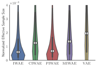
As an additional measure of the performance of the inference network that is distinct to any of the training targets, we also considered the effective sample size (ESS) (Owen, 2013) for the fully trained networks, defined as

$$\text{ESS}=(\textstyle\sum_{k=1}^{K}w_{k})^{2}/\textstyle\sum_{k=1}^{K}w_{k}^{2}.$$ (19)

The ESS is a measure of how many unweighted samples would be equivalent to the weighted sample set. A low ESS indicates that the inference network is struggling to perform effective inference for the generative network. The results, given in Figure 7, show that the ESSs for ciwae, miwae, and the vae were all significantly larger than for iwae and piwae, with iwae giving a particularly poor ESS.

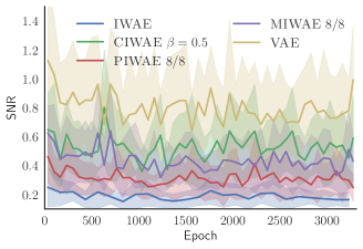
Our final experiment looks at the snr values for the inference networks during training. Here we took a number of different neural network gradient weights at different layers of the network and calculated empirical estimates for their snr s at various points during the training. We then averaged these estimates over the different network weights, the results of which are given in Figure 8. This clearly shows the low snr exhibited by the iwae inference network, suggesting that our results from the simple Gaussian experiments carry over to the more complex neural network domain.

Figure 8: snr of inference network weights during training. All lines are mean $\pm$ standard deviation over 20 randomly chosen weights per layer.

6 Conclusions

We have provided theoretical and empirical evidence that algorithmic approaches to increasing the tightness of the elbo independently to the expressiveness of the inference network can be detrimental to learning by reducing the signal-to-noise ratio of the inference network gradients. Experiments on a simple latent variable model confirmed our theoretical findings. We then exploited these insights to introduce three estimators, piwae, miwae, and ciwae and showed that each can deliver improvements over iwae, even when the metric used for this assessment is the iwae target itself. In particular, each was able to deliver improvement in the training of the inference network, without any reduction in the quality of the learned generative network.

Whereas miwae and ciwae mostly allow for balancing the requirements of the inference and generative networks, piwae appears to be able to offer simultaneous improvements to both, with the improved training of the inference network having a knock-on effect on the generative network. Key to achieving this is, is its use of separate targets for the two networks, opening up interesting avenues for future work.

 

Appendices for Tighter Variational Bounds are Not Necessarily Better

 

Tom Rainforth  Adam R. Kosiorek  Tuan Anh Le  Chris J. Maddison
Maximilian Igl  Frank Wood  Yee Whye Teh

Appendix A Proof of SNR Convergence Rates

Before proving Theorem 1, we first introduce the following lemma that will be helpful for demonstrating the result. We note that the lemma can be interpreted as a generalization on the well-known results for the third and fourth moments of Monte Carlo estimators.

Lemma 1.

Let $a_{1},\dots,a_{K}$, $b_{1},\dots,b_{K}$, and $c_{1},\dots,c_{K}$ be sets of random variables such that

• The $a_{k}$ are independent and identically distributed (i.i.d.). Similarly, the $b_{k}$ are i.i.d. and the $c_{k}$ are i.i.d.

• $\mathbb{E}[a_{k}]=\mathbb{E}[b_{k}]=\mathbb{E}[c_{k}]=0,\quad\forall k\in\{1,\dots,K\}$

• $a_{i}$, $b_{j}$, $c_{k}$ are mutually independent if $i\neq j\neq k\neq i$, but potentially dependent otherwise

Then the following results hold

$$\mathbb{E}\left[\left(\frac{1}{K}\sum_{k=1}^{K}a_{k}\right)\left(\frac{1}{K}\sum_{k=1}^{K}b_{k}\right)\left(\frac{1}{K}\sum_{k=1}^{K}c_{k}\right)\right]=\frac{1}{K^{2}}\mathbb{E}[a_{1}b_{1}c_{1}]$$ (20)

$$\textnormal{Var}\left[\left(\frac{1}{K}\sum_{k=1}^{K}a_{k}\right)\left(\frac{1}{K}\sum_{k=1}^{K}b_{k}\right)\right]=\frac{1}{K^{3}}\textnormal{Var}[a_{1}b_{1}]+\frac{K-1}{K^{3}}\mathbb{E}[a_{1}^{2}]\mathbb{E}[b_{1}^{2}]+\frac{2K-2}{K^{3}}\left(\mathbb{E}[a_{1}b_{1}]\right)^{2}.$$ (21)

Proof.

For the first result we have

$$\mathbb{E}\left[\left(\frac{1}{K}\sum_{k=1}^{K}a_{k}\right)\left(\frac{1}{K}\sum_{k=1}^{K}b_{k}\right)\left(\frac{1}{K}\sum_{k=1}^{K}c_{k}\right)\right] =\frac{1}{K^{3}}\sum_{k=1}^{K}\mathbb{E}[a_{k}b_{k}c_{k}]+\frac{1}{K^{3}}\sum_{i=1}^{K}\sum_{j=1,j\neq i}^{K}\sum_{k=1,k\neq i}^{K}\mathbb{E}[a_{i}b_{j}c_{k}]$$

$$=\frac{1}{K^{2}}\mathbb{E}[a_{1}b_{1}c_{1}]+\frac{1}{K^{3}}\sum_{i=1}^{K}\sum_{j=1,j\neq i}^{K}\sum_{k=1,k\neq i}^{K}\mathbb{E}[a_{i}]\mathbb{E}[b_{j}c_{k}]$$

$$=\frac{1}{K^{2}}\mathbb{E}[a_{1}b_{1}c_{1}]$$

as required by using the fact that $\mathbb{E}[a_{i}]=0$.

For the second result, we again use the fact that any “off-diagonal” terms for $a_{i}a_{j}b_{k}b_{\ell}$, that is terms which have the value of one index distinct to any of the others, have expectation zero to give

Var $$\left[\left(\frac{1}{K}\sum_{k=1}^{K}a_{k}\right)\left(\frac{1}{K}\sum_{k=1}^{K}b_{k}\right)\right]=\mathbb{E}\left[\left(\frac{1}{K}\sum_{k=1}^{K}a_{k}\right)^{2}\left(\frac{1}{K}\sum_{k=1}^{K}b_{k}\right)^{2}\right]-\left(\mathbb{E}\left[\left(\frac{1}{K}\sum_{k=1}^{K}a_{k}\right)\left(\frac{1}{K}\sum_{k=1}^{K}b_{k}\right)\right]\right)^{2}$$

$$=\frac{1}{K^{4}}\sum_{k=1}^{K}\mathbb{E}[a_{k}^{2}b_{k}^{2}]+\frac{1}{K^{4}}\sum_{i=1}^{K}\sum_{k=1,k\neq i}^{K}\mathbb{E}[a_{i}^{2}]\mathbb{E}[b_{k}^{2}]+\frac{2}{K^{4}}\sum_{i=1}^{K}\sum_{k=1,k\neq i}^{K}\mathbb{E}[a_{i}b_{i}]\mathbb{E}[a_{k}b_{k}]-\frac{1}{K^{3}}\left(\mathbb{E}[a_{1}b_{1}]\right)^{2}$$

$$=\frac{1}{K^{3}}\textnormal{Var}[a_{1}b_{1}]+\frac{K-1}{K^{3}}\mathbb{E}[a_{1}^{2}]\mathbb{E}[b_{1}^{2}]+\frac{2K-2}{K^{3}}\left(\mathbb{E}[a_{1}b_{1}]\right)^{2}$$

as required. ∎

Theorem 1.

Assume that when $M=K=1$, the expected gradients; the variances of the gradients; and the first four moments of $w_{1,1}$, $\nabla_{\theta}w_{1,1}$, and $\nabla_{\phi}w_{1,1}$ are all finite and the variances are also non-zero. Then the signal-to-noise ratios of the gradient estimates converge at the following rates

$$\operatorname{\lx@glossaries@gls@link{acronym}{SNR}{\leavevmode\textsc{snr}}}_{M,K}(\theta) =\sqrt{M}\left|\frac{\sqrt{K}\;\nabla_{\theta}Z-\frac{1}{2Z\sqrt{K}}\nabla_{\theta}\left(\frac{\textnormal{Var}\left[w_{1,1}\right]}{Z^{2}}\right)+O\left(\frac{1}{K^{3/2}}\right)}{\sqrt{\mathbb{E}\left[w_{1,1}^{2}\left(\nabla_{\theta}\log w_{1,1}-\nabla_{\theta}\log Z\right)^{2}\right]}+O\left(\frac{1}{K}\right)}\right|$$ (22)

$$\operatorname{\lx@glossaries@gls@link{acronym}{SNR}{\leavevmode\textsc{snr}}}_{M,K}(\phi) =\sqrt{M}\left|\frac{\nabla_{\phi}\textnormal{Var}\left[w_{1,1}\right]+O\left(\frac{1}{K}\right)}{2Z\sqrt{K}\;\sigma\left[\nabla_{\phi}w_{1,1}\right]+O\left(\frac{1}{\sqrt{K}}\right)}\right|$$ (23)

where $Z:=p_{\theta}(x)$ is the true marginal likelihood.

Proof.

We start by considering the variance of the estimators. We will first exploit the fact that each $\hat{Z}_{m,K}$ is independent and identically distributed and then apply Taylor’s theorem to $\log\hat{Z}_{m,K}$ about $Z$, using $R_{1}(\cdot)$ to indicate the remainder term, as follows.

$$M \cdot\text{Var}\left[\Delta_{M,K}\right]=\text{Var}\left[\Delta_{1,K}\right]=\text{Var}\left[\nabla_{\theta,\phi}\left(\log Z+\frac{\hat{Z}_{1,K}-Z}{Z}+R_{1}\left(\hat{Z}_{1,K}\right)\right)\right]$$

$$= \text{Var}\left[\nabla_{\theta,\phi}\left(\frac{\hat{Z}_{1,K}-Z}{Z}+R_{1}\left(\hat{Z}_{1,K}\right)\right)\right]$$

$$= \mathbb{E}\left[\left(\nabla_{\theta,\phi}\left(\frac{\hat{Z}_{1,K}-Z}{Z}+R_{1}\left(\hat{Z}_{1,K}\right)\right)\right)^{2}\right]-\left(\mathbb{E}\left[\nabla_{\theta,\phi}\left(\frac{\hat{Z}_{1,K}-Z}{Z}+R_{1}\left(\hat{Z}_{1,K}\right)\right)\right]\right)^{2}$$

$$= \mathbb{E}\left[\left(\frac{1}{K}\sum_{k=1}^{K}\frac{Z\nabla_{\theta,\phi}w_{1,k}-w_{1,k}\nabla_{\theta,\phi}Z}{Z^{2}}+\nabla_{\theta,\phi}R_{1}\left(\hat{Z}_{1,K}\right)\right)^{2}\right]-\left(\nabla_{\theta,\phi}\cancelto{0}{\mathbb{E}\left[\frac{\hat{Z}_{1,K}-Z}{Z}\right]}+\mathbb{E}\left[\nabla_{\theta,\phi}R_{1}\left(\hat{Z}_{1,K}\right)\right]\right)^{2}$$

$$\begin{split}=&\frac{1}{KZ^{4}}\mathbb{E}\left[\left(Z\nabla_{\theta,\phi}w_{1,1}-w_{1,1}\nabla_{\theta,\phi}Z\right)^{2}\right]+\text{Var}\left[\nabla_{\theta,\phi}R_{1}\left(\hat{Z}_{1,K}\right)\right]\\ &+2\mathbb{E}\left[\left(\nabla_{\theta,\phi}R_{1}\left(\hat{Z}_{1,K}\right)\right)\left(\frac{1}{K}\sum_{k=1}^{K}\frac{Z\nabla_{\theta,\phi}w_{1,k}-w_{1,k}\nabla_{\theta,\phi}Z}{Z^{2}}\right)\right]\end{split}$$ (24)

Now by the mean-value form of the remainder in Taylor’s Theorem, we have that for some $\tilde{Z}$ between $Z$ and $\hat{Z}_{1,K}$

$$R_{1}\left(\hat{Z}_{1,K}\right)=-\frac{\left(\hat{Z}_{1,K}-Z\right)^{2}}{2\tilde{Z}^{2}}$$

and therefore

$$\nabla_{\theta,\phi}R_{1}\left(\hat{Z}_{1,K}\right)=-\frac{\tilde{Z}\left(\hat{Z}_{1,K}-Z\right)\nabla_{\theta,\phi}\left(\hat{Z}_{1,K}-Z\right)-\left(\hat{Z}_{1,K}-Z\right)^{2}\nabla_{\theta,\phi}\tilde{Z}}{\tilde{Z}^{3}}.$$ (25)

By definition, $\tilde{Z}=Z+\alpha(\hat{Z}_{1,K}-Z)$ for some $0<\alpha<1$. Furthermore, the moments of $\nabla_{\theta,\phi}\alpha$ must be bounded as otherwise we would end up with non-finite moments of the overall gradients, which would, in turn, violate our assumptions. As moments of $(\hat{Z}_{1,K}-Z)$ and $\nabla_{\theta,\phi}(\hat{Z}_{1,K}-Z)$ decrease with $K$, we thus further have that $\tilde{Z}=Z+o(1)$ and $\nabla_{\theta,\phi}\tilde{Z}=\nabla_{\theta,\phi}Z+o(1)$ where $o(1)$ indicates terms that tend to zero as $K\to\infty$. By substituting these into (25) and doing a further Taylor expansion on $1/\tilde{Z}$ about $1/Z$ we now have

$$\nabla_{\theta,\phi}R_{1}\left(\hat{Z}_{1,K}\right) =-\left(\frac{1}{Z^{3}}+o(1)\right)\left(\left(Z+o(1)\right)\left(\hat{Z}_{1,K}-Z\right)\nabla_{\theta,\phi}\left(\hat{Z}_{1,K}-Z\right)-\left(\hat{Z}_{1,K}-Z\right)^{2}\left(\nabla_{\theta,\phi}Z+o(1)\right)\right)$$

$$=-\frac{1}{Z^{3}}\left(\hat{Z}_{1,K}-Z\right)\left(Z\,\nabla_{\theta,\phi}\left(\hat{Z}_{1,K}-Z\right)-\left(\hat{Z}_{1,K}-Z\right)\nabla_{\theta,\phi}Z\right)+o(\epsilon)$$

$$=\frac{1}{Z^{3}}\left(Z-\hat{Z}_{1,K}\right)\left(Z\,\nabla_{\theta,\phi}\hat{Z}_{1,K}-\hat{Z}_{1,K}\nabla_{\theta,\phi}Z\right)+o(\epsilon)$$

where $o(\epsilon)$ indicates (asymptotically dominated) higher order terms originating from the $o(1)$ terms. If we now define

$$a_{k} =\frac{Z-w_{1,k}}{Z^{3}}\quad\text{and}$$ (26)

$$b_{k} =Z\,\nabla_{\theta,\phi}w_{1,K}-w_{1,K}\nabla_{\theta,\phi}Z$$ (27)

then we have $\mathbb{E}[a_{k}]=\mathbb{E}[b_{k}]=0,\,\forall k\in\{1,\dots,K\}$ and

$$\nabla_{\theta,\phi}R_{1}\left(\hat{Z}_{1,K}\right)=\left(\frac{1}{K}\sum_{k=1}^{K}a_{k}\right)\left(\frac{1}{K}\sum_{k=1}^{K}b_{k}\right)+o(\epsilon).$$

This is in the form required by Lemma 1 and satisfies the required assumptions and so we immediately have

$$\text{Var}\left[\nabla_{\theta,\phi}R_{1}\left(\hat{Z}_{1,K}\right)\right]=\frac{1}{K^{3}}\textnormal{Var}[a_{1}b_{1}]+\frac{K-1}{K^{3}}\mathbb{E}[a_{1}^{2}]\mathbb{E}[b_{1}^{2}]+\frac{2K-2}{K^{3}}\left(\mathbb{E}[a_{1}b_{1}]\right)^{2}+o(\epsilon)=O\left(\frac{1}{K^{2}}\right)$$

by the second result in Lemma 1. If we further define

$$c_{k}=b_{k}\quad\forall k\in\{1,\dots,K\}$$ (28)

then we can also use the first result in Lemma 1 to give

$$2\mathbb{E}\left[\left(\nabla_{\theta,\phi}R_{1}\left(\hat{Z}_{1,K}\right)\right)\left(\frac{1}{K}\sum_{k=1}^{K}\frac{Z\nabla_{\theta,\phi}w_{1,k}-w_{1,k}\nabla_{\theta,\phi}Z}{Z^{2}}\right)\right]=\frac{2}{Z^{2}K^{2}}\mathbb{E}\left[a_{1}b_{1}^{2}\right]+o(\epsilon)=O\left(\frac{1}{K^{2}}\right).$$

Substituting these results back into (24) now gives

$$\text{Var}\left[\Delta_{M,K}\right]=\frac{1}{MKZ^{4}}\mathbb{E}\left[\left(Z\nabla_{\theta,\phi}w_{1,1}-w_{1,1}\nabla_{\theta,\phi}Z\right)^{2}\right]+\frac{1}{M}O\left(\frac{1}{K^{2}}\right).$$ (29)

Considering now the expected gradient estimate and again using Taylor’s theorem, this time to a higher number of terms,

$$\mathbb{E}\left[\Delta_{M,K}\right] =\mathbb{E}\left[\Delta_{1,K}\right]=\mathbb{E}\left[\Delta_{1,K}-\nabla_{\theta,\phi}\log Z\right]+\nabla_{\theta,\phi}\log Z$$

$$=\nabla_{\theta,\phi}\mathbb{E}\left[\log Z+\frac{\hat{Z}_{1,K}-Z}{Z}-\frac{\left(\hat{Z}_{1,K}-Z\right)^{2}}{2Z^{2}}+R_{2}\left(\hat{Z}_{1,K}\right)-\log Z\right]+\nabla_{\theta,\phi}\log Z$$

$$=-\frac{1}{2}\nabla_{\theta,\phi}\mathbb{E}\left[\left(\frac{\hat{Z}_{1,K}-Z}{Z}\right)^{2}\right]+\nabla_{\theta,\phi}\mathbb{E}\left[R_{2}\left(\hat{Z}_{1,K}\right)\right]+\nabla_{\theta,\phi}\log Z$$

$$=-\frac{1}{2}\nabla_{\theta,\phi}\left(\frac{\text{Var}\left[\hat{Z}_{1,K}\right]}{Z^{2}}\right)+\nabla_{\theta,\phi}\mathbb{E}\left[R_{2}\left(\hat{Z}_{1,K}\right)\right]+\nabla_{\theta,\phi}\log Z$$

$$=-\frac{1}{2K}\nabla_{\theta,\phi}\left(\frac{\text{Var}\left[w_{1,1}\right]}{Z^{2}}\right)+\nabla_{\theta,\phi}\mathbb{E}\left[R_{2}\left(\hat{Z}_{1,K}\right)\right]+\nabla_{\theta,\phi}\log Z.$$ (30)

Here we have

$$R_{2}\left(\hat{Z}_{1,K}\right)=\frac{\left(\hat{Z}_{1,K}-Z\right)^{3}}{3\check{Z}^{3}}$$

with $\check{Z}$ defined analogously to $\tilde{Z}$ but not necessarily taking on the same value. Using $\check{Z}=Z+o(1)$ and $\nabla_{\theta,\phi}\check{Z}=\nabla_{\theta,\phi}Z+o(1)$ as before and again applying a Taylor expansion about $1/Z$ now yields

$$\nabla_{\theta,\phi}\mathbb{E}\left[R_{2}\left(\hat{Z}_{1,K}\right)\right] =\nabla_{\theta,\phi}\left(\frac{1}{3Z^{3}}\mathbb{E}\left[\left(\frac{1}{K}\sum_{k=1}^{K}w_{1,k}-Z\right)^{3}\right]\right)+o(\epsilon)$$

and thus by applying Lemma 1 with $a_{k}=b_{k}=c_{k}=w_{1,k}-Z$ we have

$$\nabla_{\theta,\phi}\mathbb{E}\left[R_{2}\left(\hat{Z}_{1,K}\right)\right] =\frac{1}{K^{2}}\nabla_{\theta,\phi}\left(\frac{1}{3Z^{3}}\mathbb{E}[\left(w_{1,k}-Z\right)^{3}]\right)+o(\epsilon)=O\left(\frac{1}{K^{2}}\right).$$

Substituting this back into (30) now yields

$$\mathbb{E}\left[\Delta_{M,K}\right]=\nabla_{\theta,\phi}\log Z-\frac{1}{2K}\nabla_{\theta,\phi}\left(\frac{\text{Var}\left[w_{1,1}\right]}{Z^{2}}\right)+O\left(\frac{1}{K^{2}}\right)$$ (31)

Finally, by combing (29) and (31), and noting that $\sqrt{\frac{A}{K}+\frac{B}{K^{2}}}=\frac{A}{\sqrt{K}}+\frac{B}{2AK^{3/2}}+O\left(\frac{1}{K^{(5/2)}}\right)$, we have for $\theta$

$$\operatorname{\lx@glossaries@gls@link{acronym}{SNR}{\leavevmode\textsc{snr}}}_{M,K}(\theta) =\left|\frac{\nabla_{\theta}\log Z-\frac{1}{2K}\nabla_{\theta}\left(\frac{\text{Var}\left[w_{1,1}\right]}{Z^{2}}\right)+O\left(\frac{1}{K^{2}}\right)}{\sqrt{\frac{1}{MKZ^{4}}\mathbb{E}\left[\left(Z\nabla_{\theta}w_{1,1}-w_{1,1}\nabla_{\theta}Z\right)^{2}\right]+\frac{1}{M}O\left(\frac{1}{K^{2}}\right)}}\right|$$ (32)

$$=\sqrt{M}\left|\frac{Z^{2}\sqrt{K}\left(\nabla_{\theta}\log Z-\frac{1}{2K}\nabla_{\theta}\left(\frac{\text{Var}\left[w_{1,1}\right]}{Z^{2}}\right)\right)+O\left(\frac{1}{K^{3/2}}\right)}{\sqrt{\mathbb{E}\left[\left(Z\nabla_{\theta}w_{1,1}-w_{1,1}\nabla_{\theta}Z\right)^{2}\right]}+O\left(\frac{1}{K}\right)}\right|$$ (33)

$$=\sqrt{M}\left|\frac{\sqrt{K}\;\nabla_{\theta}Z-\frac{1}{2Z\sqrt{K}}\nabla_{\theta}\left(\frac{\text{Var}\left[w_{1,1}\right]}{Z^{2}}\right)+O\left(\frac{1}{K^{3/2}}\right)}{\sqrt{\mathbb{E}\left[w_{1,1}^{2}\left(\nabla_{\theta}\log w_{1,1}-\nabla_{\theta}\log Z\right)^{2}\right]}+O\left(\frac{1}{K}\right)}\right|=O\left(\sqrt{MK}\right).$$ (34)

For $\phi$, then because $\nabla_{\phi}Z=0$, we instead have

$$\operatorname{\lx@glossaries@gls@link{acronym}{SNR}{\leavevmode\textsc{snr}}}_{M,K}(\phi)=\sqrt{M}\left|\frac{\nabla_{\phi}\text{Var}\left[w_{1,1}\right]+O\left(\frac{1}{K}\right)}{2Z\sqrt{K}\;\sigma\left[\nabla_{\phi}w_{1,1}\right]+O\left(\frac{1}{\sqrt{K}}\right)}\right|=O\left(\sqrt{\frac{M}{K}}\right)$$ (35)

and we are done. ∎

Appendix B Derivation of Optimal Parameters for Gaussian Experiment

To derive the optimal parameters for the Gaussian experiment we first note that

$$\mathcal{J}(\theta,\phi) =\frac{1}{N}\log\prod_{n=1}^{N}p_{\theta}(x^{(n)})-\frac{1}{N}\sum_{n=1}^{N}\lx@glossaries@gls@link{acronym}{KL}{\leavevmode\textsc{kl}}\left(Q_{\phi}(z_{1:K}|x^{(n)})\middle|\middle|P_{\theta}(z_{1:K}|x^{(n)})\right)\quad\text{where}$$

$$P_{\theta}(z_{1:K}|x^{(n)}) =\frac{1}{K}\sum_{k=1}^{K}q_{\phi}(z_{1}|x^{(n)})\dots q_{\phi}(z_{k-1}|x^{(n)})p_{\theta}(z_{k}|x^{(n)})q_{\phi}(z_{k+1}|x^{(n)})\dots q_{\phi}(z_{K}|x^{(n)}),$$

$Q_{\phi}(z_{1:K}|x^{(n)})$ is as per (2) and the form of the Kullback-Leibler (kl) is taken from (Le et al., 2018). Next, we note that $\phi$ only controls the mean of the proposal so, while it is not possible to drive the KL to zero, it will be minimized for any particular $\theta$ when the means of $q_{\phi}(z|x^{(n)})$ and $p_{\theta}(z|x^{(n)})$ are the same. Furthermore, the corresponding minimum possible value of the KL is independent of $\theta$ and so we can calculate the optimum pair $(\theta^{*},\phi^{*})$ by first optimizing for $\theta$ and then choosing the matching $\phi$. The optimal $\theta$ maximizes $\log\prod_{n=1}^{N}p_{\theta}(x^{(n)})$, giving $\theta^{*}:=\mu^{*}=\frac{1}{N}\sum_{n=1}^{N}x^{(n)}$. As we straightforwardly have $p_{\theta}(z|x^{(n)})=\mathcal{N}(z;\left(x^{(n)}+\mu\right)/2,I/2)$, the KL is then minimized when $A=I/2$ and $b=\mu/2$, giving $\phi^{*}:=(A^{*},b^{*})$, where $A^{*}=I/2$ and $b^{*}=\mu^{*}/2$.

Appendix C Additional Empirical Analysis of SNR

C.1 Histograms for VAE

To complete the picture for the effect of $M$ and $K$ on the distribution of the gradients, we generated histograms for the $K=1$ (i.e. vae) gradients as $M$ is varied. As shown in Figure 9(a), we see the expected effect from the law of large numbers that the variance of the estimates decreases with $M$, but not the expected value.

(a) vae inference network gradient estimates

(b) vae generative network gradient estimates

Figure 9: Histograms of gradient estimates $\Delta_{M,K}$ for the generative network and the inference network using the vae ($K=1$) objectives with different values of $M$.

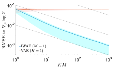
C.2 Convergence of RMSE for Generative Network

As explained in the main paper, the SNR is not an entirely appropriate metric for the generative network – a low SNR is still highly problematic, but a high SNR does not indicate good performance. It is thus perhaps better to measure the quality of the gradient estimates for the generative network by looking at the root mean squared error (rmse) to $\nabla_{\mu}\log Z$, i.e. $\sqrt{\mathbb{E}\left[\lVert\Delta_{M,K}-\nabla_{\mu}\log Z\rVert_{2}^{2}\right]}$. The convergence of this rmse is shown in Figure 10 where the solid lines are the rmse estimates using $10^{4}$ runs and the shaded regions show the interquartile range of the individual estimates. We see that increasing $M$ in the vae reduces the variance of the estimates but has negligible effect on the rmse due to the fixed bias. On the other hand, we see that increasing $K$ leads to a monotonic improvement, initially improving at a rate $O(1/K)$ (because the bias is the dominating term in this region), before settling to the standard Monte Carlo convergence rate of $O(1/\sqrt{K})$ (shown by the dashed lines).

Figure 10: RMSE in $\mu$ gradient estimate to $\nabla_{\mu}\log Z$

C.3 Experimental Results for High Variance Regime

We now present empirical results for a case where our weights are higher variance. Instead of choosing a point close to the optimum by offsetting parameters with a standard deviation of $0.01$, we instead offset using a standard deviation of $0.5$. We further increased the proposal covariance to $I$ to make it more diffuse. This is now a scenario where the model is far from its optimum and the proposal is a very poor match for the model, giving very high variance weights.

We see that the behavior is the same for variation in $M$, but somewhat distinct for variation in $K$. In particular, the snr and dsnr only decrease slowly with $K$ for the inference network, while increasing $K$ no longer has much benefit for the snr of the inference network. It is clear that, for this setup, the problem is very far from the asymptotic regime in $K$ such that our theoretical results no longer directly apply. Nonetheless, the high-level effect observed is still that the snr of the inference network deteriorates, albeit slowly, as $K$ increases.

(a) iwae inference network gradient estimates

(b) vae inference network gradient estimates

(c) iwae generative network gradient estimates

(d) vae generative network gradient estimates

Figure 11: Histograms of gradient estimates as per Figure 1.

(a) Convergence of snr for inference network

(b) Convergence of snr for generative network

Figure 12: Convergence of signal-to-noise ratios of gradient estimates as per Figure 2.

(a) Convergence of dsnr for inference network

(b) Convergence of dsnr for generative network

Figure 13: Convergence of directional signal-to-noise ratio of gradients estimates as per Figure 3.

(a) Convergence of dsnr for inference network

(b) Convergence of dsnr for generative network

Figure 14: Convergence of directional signal-to-noise ratio of gradient estimates where the true gradient is taken as $\mathbb{E}\left[\Delta_{1,1000}\right]$ as per Figure 4.

Appendix D Convergence of Deep Generative Model for Alternative Parameter Settings

Figure 15 shows the convergence of the introduced algorithms under different settings to those shown in Figure 5. Namely we consider $M=4,K=16$ for piwae and miwae and $\beta=0.05$ for ciwae. These settings all represent tighter bounds than those of the main paper. Similar behavior is seen in terms of the iwae-64 metric for all algorithms. piwae produced similar mean behavior for all metrics, though the variance was noticeably increased for $\log\hat{p}(x)$. For ciwae and miwae, we see that the parameter settings represent an explicit trade-off between the generative network and the inference network: $\log\hat{p}(x)$ was noticeably increased for both, matching that of iwae, while $-\textsc{KL}(Q_{\phi}(z\lvert x)||P_{\theta}(z\lvert x))$ was reduced. Critically, we see here that, as observed for piwae in the main paper, miwae and ciwae are able to match the generative model performance of iwae whilst improving the KL metric, indicating that they have learned better inference networks.

(a) IWAE₆₄

(b) $\log\hat{p}(x)$

(c) $-\mathrm{KL}(Q_{\phi}(z\lvert x)||P_{\theta}(z\lvert x))$

Figure 15: Convergence of different evaluation metrics for each method. Plotting conventions as per Figure 5.

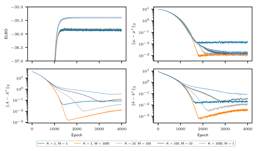
Appendix E Convergence of Toy Gaussian Problem

We finish by assessing the effect of the outlined changes in the quality of the gradient estimates on the final optimization for our toy Gaussian problem. Figure 16 shows the convergence of running Adam (Kingma & Ba, 2014) to optimize $\mu$, $A$, and $b$. This suggests that the effects observed predominantly transfer to the overall optimization problem. Interestingly, setting $K=1$ and $M=1000$ gave the best performance on learning not only the inference network parameters, but also the generative network parameters.

Figure 16: Convergence of optimization for different values of $K$ and $M$. (Top, left) $\operatorname{\lx@glossaries@gls@link{acronym}{ELBO}{\leavevmode\textsc{elbo}}}_{\text{IS}}$ during training (note this represents a different metric for different $K$). (Top, right) $L_{2}$ distance of the generative network parameters from the true maximizer. (Bottom) $L_{2}$ distance of the inference network parameters from the true maximizer. Plots show means over $3$ repeats with $\pm 1$ standard deviation. Optimization is performed using the Adam algorithm with all parameters initialized by sampling from the uniform distribution on $[1.5,2.5]$.

References

• Bamler et al. (2017) Bamler, R., Zhang, C., Opper, M., and Mandt, S. Perturbative black box variational inference. arXiv preprint arXiv:1709.07433, 2017.
• Bourlard & Kamp (1988) Bourlard, H. and Kamp, Y. Auto-association by multilayer perceptrons and singular value decomposition. Biological cybernetics, 59(4-5):291–294, 1988.
• Burda et al. (2016) Burda, Y., Grosse, R., and Salakhutdinov, R. Importance weighted autoencoders. In ICLR, 2016.
• Chen et al. (2017) Chen, X., Kingma, D. P., Salimans, T., Duan, Y., Dhariwal, P., Schulman, J., Sutskever, I., and Abbeel, P. Variational lossy autoencoder. In ICLR, 2017.
• Cremer et al. (2017) Cremer, C., Morris, Q., and Duvenaud, D. Reinterpreting importance-weighted autoencoders. arXiv preprint arXiv:1704.02916, 2017.
• Fort et al. (2017) Fort, G., Gobet, E., and Moulines, E. Mcmc design-based non-parametric regression for rare event. application to nested risk computations. Monte Carlo Methods and Applications, 23(1):21–42, 2017.
• Gregor et al. (2016) Gregor, K., Besse, F., Rezende, D. J., Danihelka, I., and Wierstra, D. Towards conceptual compression. In NIPS, 2016.
• Hesterberg (1988) Hesterberg, T. C. Advances in importance sampling. PhD thesis, Stanford University, 1988.
• Hinton & Zemel (1994) Hinton, G. E. and Zemel, R. S. Autoencoders, minimum description length and helmholtz free energy. In NIPS, 1994.
• Hoffman et al. (2013) Hoffman, M. D., Blei, D. M., Wang, C., and Paisley, J. Stochastic variational inference. The Journal of Machine Learning Research, 14(1):1303–1347, 2013.
• Kingma & Ba (2014) Kingma, D. and Ba, J. Adam: A method for stochastic optimization. arXiv preprint arXiv:1412.6980, 2014.
• Kingma & Welling (2014) Kingma, D. P. and Welling, M. Auto-encoding variational Bayes. In ICLR, 2014.
• Kingma et al. (2016) Kingma, D. P., Salimans, T., and Welling, M. Improving variational inference with inverse autoregressive flow. arXiv preprint arXiv:1606.04934, 2016.
• Le et al. (2017) Le, T. A., Baydin, A. G., and Wood, F. Inference compilation and universal probabilistic programming. In AISTATS, 2017.
• Le et al. (2018) Le, T. A., Igl, M., Rainforth, T., Jin, T., and Wood, F. Auto-encoding sequential Monte Carlo. In ICLR, 2018.
• LeCun et al. (1998) LeCun, Y., Bottou, L., Bengio, Y., and Haffner, P. Gradient-based learning applied to document recognition. Proceedings of the IEEE, 86(11):2278–2324, 1998.
• Li & Turner (2016) Li, Y. and Turner, R. E. Rényi divergence variational inference. In NIPS, 2016.
• Maaløe et al. (2016) Maaløe, L., Sønderby, C. K., Sønderby, S. K., and Winther, O. Auxiliary deep generative models. arXiv preprint arXiv:1602.05473, 2016.
• Maddison et al. (2017) Maddison, C. J., Lawson, D., Tucker, G., Heess, N., Norouzi, M., Mnih, A., Doucet, A., and Teh, Y. W. Filtering variational objectives. arXiv preprint arXiv:1705.09279, 2017.
• Naesseth et al. (2018) Naesseth, C. A., Linderman, S. W., Ranganath, R., and Blei, D. M. Variational sequential Monte Carlo. 2018.
• Owen (2013) Owen, A. B. Monte Carlo theory, methods and examples. 2013.
• Paige & Wood (2016) Paige, B. and Wood, F. Inference networks for sequential Monte Carlo in graphical models. In ICML, 2016.
• Rainforth (2017) Rainforth, T. Automating Inference, Learning, and Design using Probabilistic Programming. PhD thesis, 2017.
• Rainforth et al. (2018) Rainforth, T., Cornish, R., Yang, H., Warrington, A., and Wood, F. On nesting Monte Carlo estimators. In ICML, 2018.
• Ranganath et al. (2014) Ranganath, R., Gerrish, S., and Blei, D. Black box variational inference. In AISTATS, 2014.
• Ranganath et al. (2016) Ranganath, R., Tran, D., and Blei, D. Hierarchical variational models. In ICML, 2016.
• Rezende & Mohamed (2015) Rezende, D. and Mohamed, S. Variational inference with normalizing flows. In International Conference on Machine Learning, pp. 1530–1538, 2015.
• Rezende et al. (2014) Rezende, D. J., Mohamed, S., and Wierstra, D. Stochastic backpropagation and approximate inference in deep generative models. In ICML, 2014.
• Roberts & Tedrake (2009) Roberts, J. W. and Tedrake, R. Signal-to-noise ratio analysis of policy gradient algorithms. In NIPS, 2009.
• Salimans et al. (2015) Salimans, T., Kingma, D., and Welling, M. Markov chain Monte Carlo and variational inference: Bridging the gap. In Proceedings of the 32nd International Conference on Machine Learning (ICML-15), pp.  1218–1226, 2015.
• Tran et al. (2015) Tran, D., Ranganath, R., and Blei, D. M. The variational Gaussian process. arXiv preprint arXiv:1511.06499, 2015.
• Turner & Sahani (2011) Turner, R. E. and Sahani, M. Two problems with variational expectation maximisation for time-series models. Bayesian Time series models, pp.  115–138, 2011.