Classification from Pairwise Similarity and Unlabeled Data

Abstract

Supervised learning needs a huge amount of labeled data, which can be a big bottleneck under the situation where there is a privacy concern or labeling cost is high. To overcome this problem, we propose a new weakly-supervised learning setting where only similar (S) data pairs (two examples belong to the same class) and unlabeled (U) data points are needed instead of fully labeled data, which is called SU classification. We show that an unbiased estimator of the classification risk can be obtained only from SU data, and the estimation error of its empirical risk minimizer achieves the optimal parametric convergence rate. Finally, we demonstrate the effectiveness of the proposed method through experiments.

1 Introduction

In supervised classification, we need a vast amount of labeled data in the training phase. However, in many real-world problems, it is time-consuming and laborious to label a huge amount of unlabeled data. To deal with this problem, weakly-supervised classification (Zhou, 2018) has been explored in various setups, including semi-supervised classification (Chapelle & Zien, 2005; Belkin et al., 2006; Chapelle et al., 2010; Miyato et al., 2016; Laine & Aila, 2017; Sakai et al., 2017; Tarvainen & Valpola, 2017; Luo et al., 2018), multiple instance classification (Li & Vasconcelos, 2015; Miech et al., 2017; Bao et al., 2018), and positive-unlabeled (PU) classification (Elkan & Noto, 2008; du Plessis et al., 2014, 2015; Niu et al., 2016; Kiryo et al., 2017).

Another line of research from the clustering viewpoint is semi-supervised clustering, where pairwise similarity and dissimilarity data (a.k.a. must-link and cannot-link constraints) are utilized to guide unsupervised clustering to a desired solution. The common approaches are (i) constrained clustering (Wagstaff et al., 2001; Basu et al., 2002, 2004; Li & Liu, 2009), which utilize pairwise links as constraints on clustering. (ii) metric learning (Xing et al., 2002; Bilenko et al., 2004; Weinberger et al., 2005; Davis et al., 2007; Li et al., 2008; Niu et al., 2012), which perform ($k$-means) clustering on learned metrics (iii) matrix completion (Yi et al., 2013; Chiang et al., 2015), which recover unknown entries in a similarity matrix.

Table 1: Explanations of classification and clustering.

Problem	Explanation
Classification	The goal is to minimize the true risk (given the zero-one loss) of an inductive classifier. To this end, an empirical risk (given a surrogate loss) on the training data is minimized for training the classifier. The training and testing phases can be clearly distinguished. Classification requires the existence of the underlying joint density.
Clustering	The goal is to partition the data at hand into clusters. To this end, density-/margin-/information-based measures are optimized for implementing the low-density separation based on the cluster assumption. Most of the clustering methods are designed for in-sample inference. Clustering does not need the underlying joint density.

Semi-supervised clustering and weakly-supervised classification are similar in that they do not use fully-supervised data. However, they are different from the learning theoretic viewpoint—weakly-supervised classification methods are justified as supervised learning methods, while semi-supervised clustering methods are still evaluated as unsupervised learning (see Table 1). Indeed, weakly-supervised learning methods based on empirical risk minimization (du Plessis et al., 2014, 2015; Niu et al., 2016; Sakai et al., 2017) were shown that their estimation errors achieve the optimal parametric convergence rate, while such generalization guarantee is not available for semi-supervised clustering methods.

The goal of this paper is to propose a novel weakly-supervised learning method called SU classification, where only similar (S) data pairs (two examples belong to the same class) and unlabeled (U) data points are employed, in order to bridge these two different paradigms. In SU classification, the information available for training a classifier is similar to semi-supervised clustering. However, our proposed method gives an inductive model, which learns decision functions from training data and can be applied for out-of-sample prediction (i.e., prediction of unseen test data). Furthermore, the proposed method can not only separate two classes but also identify which class is positive (class identification) under certain conditions.

SU classification is particularly useful to predict people’s sensitive matters such as religion, politics, and opinions on racial issues—people often hesitate to give explicit answers to these matters, instead indirect questions might be easier to answer: “Which person do you have the same belief as?”

For this SU classification problem, our contributions in this paper are three-fold:

1. We propose an empirical risk minimization method for SU classification (Section 2). This enables us to obtain an inductive classifier. Under certain loss conditions together with the linear-in-parameter model, its objective function becomes even convex in the parameters.

2. We theoretically establish an estimation error bound for our SU classification method (Section 4), showing that the proposed method achieves the optimal parametric convergence rate.

3. We experimentally demonstrate the practical usefulness of the proposed SU classification method (Section 5).

Related problem settings are summarized in Figure 1.

Figure 1: Illustrations of SU classification and other related problem settings.

2 Classification from Pairwise Similarity and Unlabeled Data

In this section, we propose a learning method to train a classifier from pairwise similarity and unlabeled data.

2.1 Preliminaries

We formulate the standard binary classification problem briefly. Let $\mathcal{X}\subset\mathbb{R}^{d}$ be a $d$-dimensional example space and $\mathcal{Y}=\{+1,-1\}$ be a binary label space. We assume that labeled data $(\bm{x},y)\in\mathcal{X}\times\mathcal{Y}$ is drawn from the joint probability distribution with density $p(\bm{x},y)$. The goal of binary classification is to obtain a classifier $f:\mathcal{X}\rightarrow\mathbb{R}$ which minimizes the classification risk defined as

$$R(f)\triangleq\mathop{\mathbb{E}}_{(X,Y)\sim p}\left[\ell(f(X),Y)\right],$$ (1)

where $\mathbb{E}_{(X,Y)\sim p}[\cdot]$ denotes the expectation over the joint distribution $p(X,Y)$ and $\ell:\mathbb{R}\times\mathcal{Y}\rightarrow\mathbb{R}_{+}$ is a loss function. The loss function $\ell(z,t)$ measures how well the true class label $t\in\mathcal{Y}$ is estimated by an output of a classifier $z\in\mathbb{R}$, generally yielding a small/large value if $t$ is well/poorly estimated by $z$.

In standard supervised classification scenarios, we are given positive and negative training data independently following $p(\bm{x},y)$. Then, based on these training data, the classification risk (1) is empirically approximated and the empirical risk minimizer is obtained. However, in many real-world problems, collecting labeled training data is costly. The goal of this paper is to train a binary classifier only from pairwise similarity and unlabeled data, which are cheaper to collect than fully labeled data.

2.2 Pairwise Similarity and Unlabeled Data

First, we discuss underlying distributions of similar data pairs and unlabeled data points, in order to perform the empirical risk minimization.

Pairwise Similarity: If $\bm{x}$ and $\bm{x}^{\prime}$ belong to the same class, they are said to be pairwise similar (S). We assume that similar data pairs are drawn following

$$p_{\mathrm{S}}(\bm{x},\bm{x}^{\prime}) =p(\bm{x},\bm{x}^{\prime}|y=y^{\prime}=+1\vee y=y^{\prime}=-1)$$

$$=\frac{\pi_{+}^{2}p_{+}(\bm{x})p_{+}(\bm{x}^{\prime})+\pi_{-}^{2}p_{-}(\bm{x})p_{-}(\bm{x}^{\prime})}{\pi_{+}^{2}+\pi_{-}^{2}},$$ (2)

where $\pi_{+}\triangleq p(y=+1)$ and $\pi_{-}\triangleq p(y=-1)$ are the class-prior probabilities satisfying $\pi_{+}+\pi_{-}=1$, and $p_{+}(\bm{x})\triangleq p(\bm{x}|y=+1)$ and $p_{-}(\bm{x})\triangleq p(\bm{x}|y=-1)$ are the class-conditional densities. Eq. (2) means that we draw two labeled data independently following $p(\bm{x},y)$, and we accept/reject them if they belong to the same class/different classes.

Unlabeled Data: We assume that unlabeled (U) data points are drawn following the marginal density $p(\bm{x})$, which can be decomposed into the sum of the class-conditional densities as

$$p(\bm{x}) =\pi_{+}p_{+}(\bm{x})+\pi_{-}p_{-}(\bm{x}).$$ (3)

Our goal is to train a classifier only from SU data, which we call SU classification. We assume that we have similar pairs $\mathcal{D}_{\mathrm{S}}$ and an unlabeled dataset $\mathcal{D}_{\mathrm{U}}$ as

$$\mathcal{D}_{\mathrm{S}} \triangleq\{(\bm{x}_{\mathrm{S},i},\bm{x}_{\mathrm{S},i}^{\prime})\}_{i=1}^{n_{\mathrm{S}}} \stackrel{{\scriptstyle\text{i.i.d.}}}{{\sim}}p_{\mathrm{S}}(\bm{x},\bm{x}^{\prime}),$$

$$\mathcal{D}_{\mathrm{U}} \triangleq\{\bm{x}_{\mathrm{U},i}\}_{i=1}^{n_{\mathrm{U}}} \stackrel{{\scriptstyle\text{i.i.d.}}}{{\sim}}p(\bm{x}).$$

We also use a notation $\widetilde{\mathcal{D}}_{\mathrm{S}}\triangleq\{\widetilde{\bm{x}}_{\mathrm{S},i}\}_{i=1}^{2n_{\mathrm{S}}}$ to denote pointwise similar data obtained by ignoring pairwise relations in $\mathcal{D}_{\mathrm{S}}$.

Lemma 1.

$\widetilde{\mathcal{D}}_{\mathrm{S}}=\{\widetilde{\bm{x}}_{\mathrm{S},i}\}_{i=1}^{2n_{\mathrm{S}}}$ are independently drawn following

$$\widetilde{p}_{\mathrm{S}}(\bm{x})=\frac{\pi_{+}^{2}p_{+}(\bm{x})+\pi_{-}^{2}p_{-}(\bm{x})}{\pi_{\mathrm{S}}},$$ (4)

where $\pi_{\mathrm{S}}\triangleq\pi_{+}^{2}+\pi_{-}^{2}$.

A proof is given in Appendix A.

Lemma 1 states that a similar data pair $(\bm{x}_{\mathrm{S}},\bm{x}_{\mathrm{S}}^{\prime})$ is essentially symmetric, and $\bm{x}_{\mathrm{S}},\bm{x}_{\mathrm{S}}^{\prime}$ can be regarded as being independently drawn following $\widetilde{p}_{\mathrm{S}}$, if we assume the pair $(\bm{x}_{\mathrm{S}},\bm{x}_{\mathrm{S}}^{\prime})$ is drawn following $p_{\mathrm{S}}$. This perspective is important when we analyze the variance of the risk estimator (Section 2.4), and estimate the class-prior (Section 3.2).

2.3 Risk Expression with SU Data

Below, we attempt to express the classification risk (1) only in terms of SU data. Assume $\pi_{+}\neq\frac{1}{2}$, and let $\widetilde{\ell}(z)$, $\mathcal{L}_{\mathrm{S},\ell}(z)$ and $\mathcal{L}_{\mathrm{U},\ell}(z)$ be

$$\widetilde{\ell}(z) \triangleq\ell(z,+1)-\ell(z,-1),$$

$$\mathcal{L}_{\mathrm{S},\ell}(z) \triangleq\frac{1}{2\pi_{+}-1}\widetilde{\ell}(z),$$

$$\mathcal{L}_{\mathrm{U},\ell}(z) \triangleq-\frac{\pi_{-}}{2\pi_{+}-1}\ell(z,+1)+\frac{\pi_{+}}{2\pi_{+}-1}\ell(z,-1).$$

Then we have the following theorem.

Theorem 1.

The classification risk (1) can be equivalently expressed as

$$R_{\mathrm{SU},\ell}(f) =\pi_{\mathrm{S}}\mathop{\mathbb{E}}_{(X,X^{\prime})\sim p_{\mathrm{S}}}\left[\frac{\mathcal{L}_{\mathrm{S},\ell}(f(X))+\mathcal{L}_{\mathrm{S},\ell}(f(X^{\prime}))}{2}\right]$$

$$\quad+\mathop{\mathbb{E}}_{X\sim p}\left[\mathcal{L}_{\mathrm{U},\ell}(f(X))\right].$$

A proof is given in Appendix B.

(a) Squared Loss, $\pi_{+}=\frac{3}{4}$

(b) Logistic Loss, $\pi_{+}=\frac{3}{4}$

(c) Squared Loss, $\pi_{+}=\frac{1}{4}$

(d) Logistic Loss, $\pi_{+}=\frac{1}{4}$

Figure 2: $\mathcal{L}_{\mathrm{S},\ell}$ and $\mathcal{L}_{\mathrm{U},\ell}$ appearing in Eq. (5) are illustrated with different loss functions and class-priors.

According to Theorem 1, the following is a natural candidate for an unbiased estimator of the classification risk (1):

$$\widehat{R} {}_{\mathrm{SU},\ell}(f)$$

$$=\frac{\pi_{\mathrm{S}}}{n_{\mathrm{S}}}\sum_{i=1}^{n_{\mathrm{S}}}\frac{\mathcal{L}_{\mathrm{S},\ell}(f(\bm{x}_{\mathrm{S},i}))+\mathcal{L}_{\mathrm{S},\ell}(f(\bm{x}_{\mathrm{S},i}^{\prime}))}{2}$$

$$\qquad+\frac{1}{n_{\mathrm{U}}}\sum_{i=1}^{n_{\mathrm{U}}}\mathcal{L}_{\mathrm{U},\ell}(f(\bm{x}_{\mathrm{U},i}))$$

$$=\frac{\pi_{\mathrm{S}}}{2n_{\mathrm{S}}}\sum_{i=1}^{2n_{\mathrm{S}}}\mathcal{L}_{\mathrm{S},\ell}(f(\widetilde{\bm{x}}_{\mathrm{S},i}))+\frac{1}{n_{\mathrm{U}}}\sum_{i=1}^{n_{\mathrm{U}}}\mathcal{L}_{\mathrm{U},\ell}(f(\bm{x}_{\mathrm{U},i})),$$ (5)

where in the last line we use the decomposed version of similar pairs $\widetilde{\mathcal{D}}_{\mathrm{S}}$ instead of $\mathcal{D}_{\mathrm{S}}$, since the loss form is symmetric.

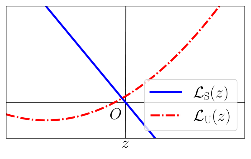
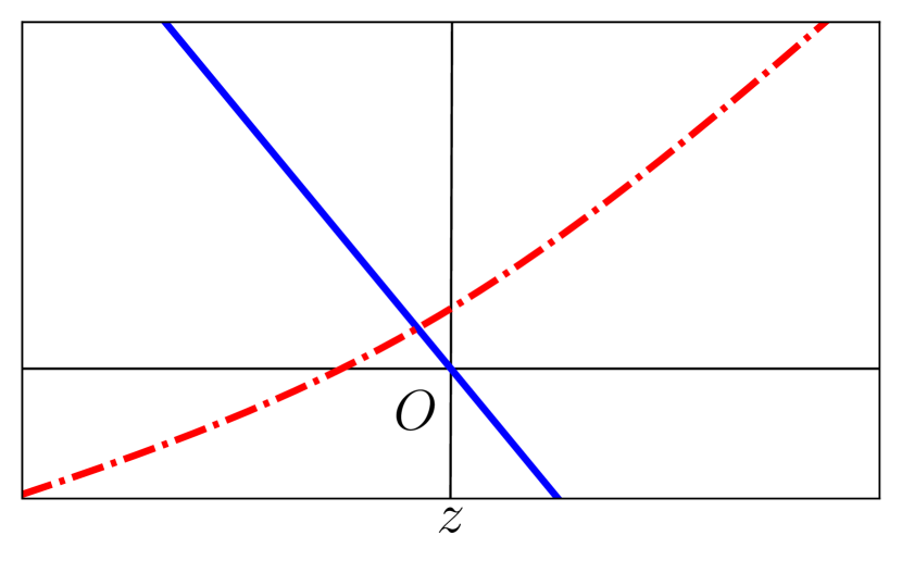
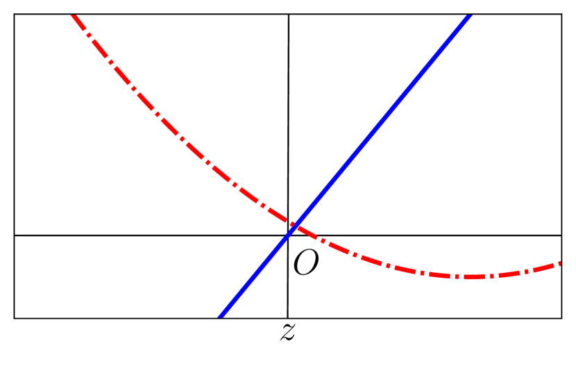
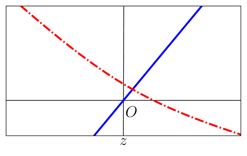
$\mathcal{L}_{\mathrm{S},\ell}$ and $\mathcal{L}_{\mathrm{U},\ell}$ are illustrated in Figure 2.

2.4 Minimum-Variance Risk Estimator

Eq. (5) is one of the candidates of an unbiased SU risk estimator. Indeed, due to the symmetry of $(\bm{x},\bm{x}^{\prime})\sim p_{\mathrm{S}}(\bm{x},\bm{x}^{\prime})$, we have the following lemma.

Lemma 2.

The first term of $R_{\mathrm{SU},\ell}(f)$, i.e.,

$$\pi_{\mathrm{S}}\mathop{\mathbb{E}}_{(X,X^{\prime})\sim p_{\mathrm{S}}}\left[\frac{\mathcal{L}_{\mathrm{S},\ell}(f(X))+\mathcal{L}_{\mathrm{S},\ell}(f(X^{\prime}))}{2}\right],$$ (6)

can be equivalently expressed as

$$\pi_{\mathrm{S}}\mathop{\mathbb{E}}_{(X,X^{\prime})\sim p_{\mathrm{S}}}\left[\alpha\mathcal{L}_{\mathrm{S},\ell}(f(X))+(1-\alpha)\mathcal{L}_{\mathrm{S},\ell}(f(X^{\prime}))\right],$$

where $\alpha\in[0,1]$ is an arbitrary weight.

A proof is given in Appendix C.1. By Lemma 2,

$$\frac{\pi_{\mathrm{S}}}{n_{\mathrm{S}}}\sum_{i=1}^{n_{\mathrm{S}}}\left\{\alpha\mathcal{L}_{\mathrm{S},\ell}(f(\bm{x}_{\mathrm{S},i}))+(1-\alpha)\mathcal{L}_{\mathrm{S},\ell}(f(\bm{x}_{\mathrm{S},i}^{\prime}))\right\}$$ (7)

is also an unbiased estimator of Eq. (6). Then, a natural question arises: is the risk estimator (5) best among all $\alpha$? We answer this question by the following theorem.

Theorem 2.

The estimator

$$\frac{\pi_{\mathrm{S}}}{n_{\mathrm{S}}}\sum_{i=1}^{n_{\mathrm{S}}}\frac{\mathcal{L}_{\mathrm{S},\ell}(f(\bm{x}_{\mathrm{S},i}))+\mathcal{L}_{\mathrm{S},\ell}(f(\bm{x}_{\mathrm{S},i}^{\prime}))}{2}$$ (8)

has the minimum variance among estimators in the form Eq. (7) with respect to $\alpha\in[0,1]$.

A proof is given in Appendix C.2.

Thus, the variance minimality (with respect to $\alpha$ in Eq. (7)) of the risk estimator (5) is guaranteed by Theorem 2. We use this risk estimator in the following sections.

2.5 Practical Implementation

Here, we investigate the objective function when the linear-in-parameter model $f(\bm{x})=\bm{w}^{\top}\bm{\phi}(\bm{x})+w_{0}$ is employed as a classifier, where $\bm{w}\in\mathbb{R}^{d}$ and $w_{0}\in\mathbb{R}$ are parameters and $\bm{\phi}:\mathbb{R}^{d}\rightarrow\mathbb{R}^{b}$ is basis functions. In general, the bias parameter $w_{0}$ can be ignored . We formulate SU classification as the following empirical risk minimization problem using Eq. (5) together with the $\ell_{2}$ regularization:

$$\widehat{\bm{w}}=\min_{\bm{w}}\widehat{J}_{\ell}(\bm{w}),$$ (9)

where

$$\widehat{J}_{\ell}(\bm{w}) \triangleq\frac{\pi_{\mathrm{S}}}{2n_{\mathrm{S}}}\sum_{i=1}^{2n_{\mathrm{S}}}\mathcal{L}_{\mathrm{S},\ell}(\bm{w}^{\top}\bm{\phi}(\widetilde{\bm{x}}_{\mathrm{S},i}))$$

$$\phantom{(\pi_{+}}+\frac{1}{n_{\mathrm{U}}}\sum_{i=1}^{n_{\mathrm{U}}}\mathcal{L}_{\mathrm{U},\ell}(\bm{w}^{\top}\bm{\phi}(\bm{x}_{\mathrm{U},i}))+\frac{\lambda}{2}\|\bm{w}\|^{2},$$ (10)

and $\lambda>0$ is the regularization parameter. We need the class-prior $\pi_{+}$ (included in $\pi_{\mathrm{S}}$) to solve this optimization problem. We discuss how to estimate $\pi_{+}$ in Section 3.2.

Next, we will investigate appropriate choices of the loss function $\ell$. From now on, we focus on margin loss functions (Mohri et al., 2012): $\ell$ is said to be a margin loss function if there exists $\psi:\mathbb{R}\rightarrow\mathbb{R}_{+}$ such that $\ell(z,t)=\psi(tz)$.

In general, our objective function (10) is non-convex even if a convex loss function is used for $\ell$ . However, the next theorem, inspired by Natarajan et al. (2013) and du Plessis et al. (2015), states that a certain loss function will result in a convex objective function.

Theorem 3.

If the loss function $\ell(z,t)$ is a convex margin loss, twice differentiable in $z$ almost everywhere (for every fixed $t\in\{\pm 1\}$), and satisfies the condition

$$\ell(z,+1)-\ell(z,-1)=-z,$$

then $\widehat{J}_{\ell}(\bm{w})$ is convex.

A proof of Theorem 3 is given in Appendix D.

Table 2: A selected list of margin loss functions satisfying the conditions in Theorem 3.

Loss name	$\psi(m)$
Squared loss	$\frac{1}{4}(m-1)^{2}$
Logistic loss	$\log(1+\exp(-m))$
Double hinge loss	$\max(-m,\max(0,\frac{1}{2}-\frac{1}{2}m))$

Examples of margin loss functions satisfying the conditions in Theorem 3 are shown in Table 2 (also illustrated in Figure 3). Below, as special cases, we show the objective functions for the squared and the double-hinge losses. The detailed derivations are given in Appendix E.

Figure 3: Comparison of loss functions.

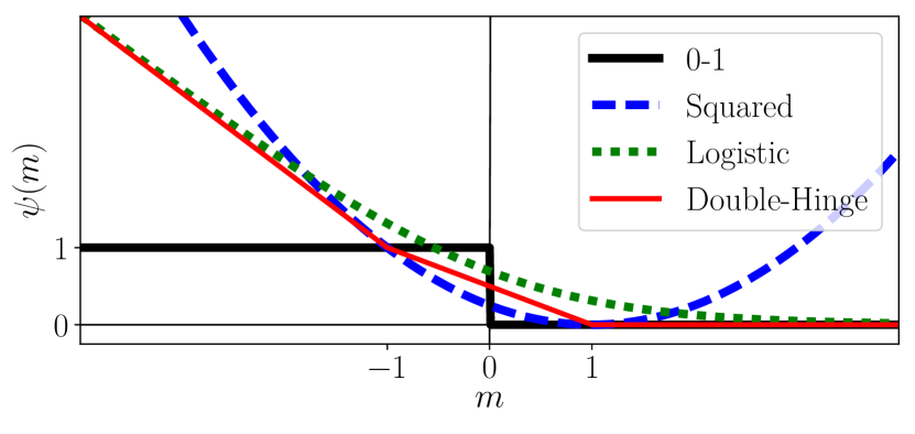
Squared Loss: The squared loss is $\ell_{\mathrm{SQ}}(z,t)=\frac{1}{4}(tz-1)^{2}$. Substituting $\ell_{\mathrm{SQ}}$ into Eq. (10), the objective function is

$$\widehat{J}_{\mathrm{SQ}}(\bm{w}) =\bm{w}^{\top}\left(\frac{1}{4n_{\mathrm{U}}}X_{\mathrm{U}}^{\top}X_{\mathrm{U}}+\frac{\lambda}{2}I\right)\bm{w}$$

$$\quad+\frac{1}{2\pi_{+}-1}\left(-\frac{\pi_{\mathrm{S}}}{2n_{\mathrm{S}}}\bm{1}^{\top}X_{\mathrm{S}}+\frac{1}{2n_{\mathrm{U}}}\bm{1}^{\top}X_{\mathrm{U}}\right)\bm{w},$$

where $\bm{1}$ is the vector whose elements are all ones, $I$ is the identity matrix, $X_{\mathrm{S}}\triangleq[\bm{\phi}(\widetilde{\bm{x}}_{\mathrm{S},1})\;\cdots\;\bm{\phi}(\widetilde{\bm{x}}_{\mathrm{S},2n_{\mathrm{S}}})]^{\top}$, and $X_{\mathrm{U}}\triangleq[\bm{\phi}(\bm{x}_{\mathrm{U},1})\;\cdots\;\bm{\phi}(\bm{x}_{\mathrm{U},n_{\mathrm{U}}})]^{\top}$. The minimizer of this objective function can be obtained analytically as

$$\bm{w} =\frac{n_{\mathrm{U}}}{2\pi_{+}-1}$$

$$\cdot\left(X_{\mathrm{U}}^{\top}X_{\mathrm{U}}+2\lambda n_{\mathrm{U}}I\right)^{-1}\left(\frac{\pi_{\mathrm{S}}}{n_{\mathrm{S}}}X_{\mathrm{S}}^{\top}\bm{1}-\frac{1}{n_{\mathrm{U}}}X_{\mathrm{U}}^{\top}\bm{1}\right).$$

Thus the optimization problem can be easily implemented and solved highly efficiently if the number of basis functions is not so large.

Double-Hinge Loss: Since the hinge loss $\ell_{\mathrm{H}}(z,t)=\max(0,1-tz)$ does not satisfy the conditions in Theorem 3, the double-hinge loss $\ell_{\mathrm{DH}}(z,t)=\max(-tz,\max(0,\frac{1}{2}-\frac{1}{2}tz))$ is proposed by du Plessis et al. (2015) as an alternative. Substituting $\ell_{\mathrm{DH}}$ into Eq. (10), we can reformulate the optimization problem as follows:

$$\min_{\bm{w},\bm{\xi},\bm{\eta}} -\frac{\pi_{\mathrm{S}}}{2n_{\mathrm{S}}(2\pi_{+}-1)}\bm{1}^{\top}X_{\mathrm{S}}\bm{w}-\frac{\pi_{-}}{n_{\mathrm{S}}(2\pi_{+}-1)}\bm{1}^{\top}\bm{\xi}$$

$$+\frac{\pi_{+}}{n_{\mathrm{U}}(2\pi_{+}-1)}\bm{1}^{\top}\bm{\eta}+\frac{\lambda}{2}\bm{w}^{\top}\bm{w}$$

s.t. $$\bm{\xi}\geq\bm{0},\quad\bm{\xi}\geq\frac{1}{2}\bm{1}+\frac{1}{2}X_{\mathrm{U}}\bm{w},\quad\bm{\xi}\geq X_{\mathrm{U}}\bm{w},$$

$$\bm{\eta}\geq\bm{0},\quad\bm{\eta}\geq\frac{1}{2}\bm{1}-\frac{1}{2}X_{\mathrm{U}}\bm{w},\quad\bm{\eta}\geq-X_{\mathrm{U}}\bm{w},$$

where $\geq$ for vectors denotes the element-wise inequality. This optimization problem is a quadratic program (QP). The transformation into the standard QP form is given in Appendix E.

3 Relation between Class-Prior and SU Classification

In Section 2, we assume that the class-prior $\pi_{+}$ is given in advance. In this section, we first clarify the relation between behaviors of the proposed method and $\pi_{+}$, then we propose an algorithm to estimate $\pi_{+}$ in case we do not have $\pi_{+}$ in advance.

3.1 Class-Prior-Dependent Behaviors of Proposed Method

We discuss the following three different cases on prior knowledge of $\pi_{+}$ (summarized in Table 3).

Table 3: Behaviors of the proposed method on class identification and class separation, depending on prior knowledge of the class-prior.

Case	Prior knowledge	Identification	Separation
1	exact $\pi_{+}$	✓	✓
2	nothing	✗	✓
3	$\mathrm{sign}(\pi_{+}-\pi_{-})$	✓	✓

(Case 1) The class-prior is given: In this case, we can directly solve the optimization problem (9). The solution does not only separate data but also identifies classes, i.e., determine which class is positive.

(Case 2) No prior knowledge on the class-prior is given: In this case, we need to estimate $\pi_{+}$ before solving (9). If we assume $\pi_{+}>\pi_{-}$, the estimation method in Section 3.2 gives an estimator of $\pi_{+}$. Thus, we can regard the larger cluster as positive class and solve the optimization problem (9). This time the solution just separates data because we have no prior information for class identifiability.

(Case 3) Magnitude relation of the class-prior is given: Finally, consider the case where we know which class has a larger class-prior. In this case, we also need to estimate $\pi_{+}$, but surprisingly, we can identify classes. For example, if the negative class has a larger class-prior, first we estimate the class-prior (let $\widehat{\pi}$ be an estimated value). Since Algorithm 1 given in Sec. 3.2 always gives an estimate of the class-prior of the larger class, the positive class-prior is given as $\pi_{+}=1-\widehat{\pi}$. After that, it reduces to Case 1.

Remark: In all of the three cases above, our proposed method gives an inductive model, which is applicable to out-of-sample prediction without any modification. On the other hand, most of the unsupervised/semi-supervised clustering methods are designed for in-sample prediction, which can only give predictions for data at hand given in advance.

3.2 Class-Prior Estimation from Pairwise Similarity and Unlabeled Data

We propose a class-prior estimation algorithm only from SU data. First, let us begin with connecting the pairwise marginal distribution $p(\bm{x},\bm{x}^{\prime})$ and $p_{\mathrm{S}}(\bm{x},\bm{x}^{\prime})$ when two examples $\bm{x}$ and $\bm{x}^{\prime}$ are drawn independently:

$$p (\bm{x},\bm{x}^{\prime})=p(\bm{x})p(\bm{x}^{\prime})$$

$$=\pi_{+}^{2}p_{+}(\bm{x})p_{+}(\bm{x}^{\prime})+\pi_{-}^{2}p_{-}(\bm{x})p_{-}(\bm{x}^{\prime})$$

$$\qquad\pi_{+}\pi_{-}p_{+}(\bm{x})p_{-}(\bm{x}^{\prime})+\pi_{+}\pi_{-}p_{-}(\bm{x})p_{+}(\bm{x}^{\prime})$$

$$=\pi_{\mathrm{S}}p_{\mathrm{S}}(\bm{x},\bm{x}^{\prime})+\pi_{\mathrm{D}}p_{\mathrm{D}}(\bm{x},\bm{x}^{\prime}),$$ (11)

where Eq. (2) was used to derive the last line, $\pi_{\mathrm{D}}\triangleq 2\pi_{+}\pi_{-}$, and

$$p {}_{\mathrm{D}}(\bm{x},\bm{x}^{\prime})$$

$$=p(\bm{x},\bm{x}^{\prime}|(y=+1\wedge y^{\prime}=-1)\vee(y=-1\wedge y^{\prime}=+1))$$

$$=\frac{\pi_{+}\pi_{-}p_{+}(\bm{x})p_{-}(\bm{x}^{\prime})+\pi_{+}\pi_{-}p_{-}(\bm{x})p_{+}(\bm{x}^{\prime})}{2\pi_{+}\pi_{-}}.$$ (12)

Marginalizing out $\bm{x}^{\prime}$ in Eq. (11) as Lemma 1, we obtain

$$p(\bm{x})=\pi_{\mathrm{S}}\widetilde{p}_{\mathrm{S}}(\bm{x})+\pi_{\mathrm{D}}\widetilde{p}_{\mathrm{D}}(\bm{x}),$$

where $\widetilde{p}_{\mathrm{S}}$ is defined in Eq. (4) and $\widetilde{p}_{\mathrm{D}}(\bm{x})\triangleq(p_{+}(\bm{x})+p_{-}(\bm{x}))/2$. Since we have samples $\mathcal{D}_{\mathrm{U}}$ and $\widetilde{\mathcal{D}}_{\mathrm{S}}$ drawn from $p$ and $\widetilde{p}_{\mathrm{S}}$ respectively (see Eqs. (3) and (4)), we can estimate $\pi_{\mathrm{S}}$ by mixture proportion estimation methods (Scott, 2015; Ramaswamy et al., 2016; du Plessis et al., 2017).

After estimating $\pi_{\mathrm{S}}$, we can calculate $\pi_{+}$. By the discussion in Section 3.1, we assume $\pi_{+}>\pi_{-}$. Then, following $2\pi_{\mathrm{S}}-1=\pi_{\mathrm{S}}-\pi_{\mathrm{D}}=(\pi_{+}-\pi_{-})^{2}=(2\pi_{+}-1)^{2}\geq 0$, we obtain $\pi_{+}=\frac{\sqrt{2\pi_{\mathrm{S}}-1}+1}{2}$. We summarize a wrapper of mixture proportion estimation in Algorithm 1.

Algorithm 1 Prior estimation from SU data. CPE is a class-prior estimation algorithm.

0:  $\mathcal{D}_{\mathrm{U}}=\{\bm{x}_{\mathrm{U},i}\}_{i=1}^{n_{\mathrm{U}}}$ (samples from $p$), $\widetilde{\mathcal{D}}_{\mathrm{S}}=\{\widetilde{\bm{x}}_{\mathrm{S},i}\}_{i=1}^{2n_{\mathrm{S}}}$ (samples from $\widetilde{p}_{\mathrm{S}}$)

0:  class-prior $\pi_{+}$

  $\pi_{\mathrm{S}}\leftarrow\texttt{CPE}(\mathcal{D}_{\mathrm{U}},\widetilde{\mathcal{D}}_{\mathrm{S}})$

  $\pi_{+}\leftarrow\frac{\sqrt{2\pi_{\mathrm{S}}-1}+1}{2}$

4 Estimation Error Bound

In this section, we establish an estimation error bound for the proposed method. Hereafter, let $\mathcal{F}\subset\mathbb{R}^{\mathcal{X}}$ be a function class of a specified model.

Definition 1.

Let $n$ be a positive integer, $Z_{1},\dots,Z_{n}$ be i.i.d. random variables drawn from a probability distribution with density $\mu$, $\mathcal{H}=\{h:\mathcal{Z}\rightarrow\mathbb{R}\}$ be a class of measurable functions, and $\bm{\sigma}=(\sigma_{1},\dots,\sigma_{n})$ be Rademacher variables, i.e., random variables taking $+1$ and $-1$ with even probabilities. Then (expected) Rademacher complexity of $\mathcal{H}$ is defined as

$$\mathfrak{R}(\mathcal{H};n,\mu)\triangleq\mathop{\mathbb{E}}_{Z_{1},\dots,Z_{n}\sim\mu}\mathop{\mathbb{E}}_{\bm{\sigma}}\left[\sup_{h\in\mathcal{H}}\frac{1}{n}\sum_{i=1}^{n}\sigma_{i}h(Z_{i})\right].$$

In this section, we assume for any probability density $\mu$, our model class $\mathcal{F}$ satisfies

$$\mathfrak{R}(\mathcal{F};n,\mu)\leq\frac{C_{\mathcal{F}}}{\sqrt{n}}$$ (13)

for some constant $C_{\mathcal{F}}>0$. This assumption is reasonable because many model classes such as the linear-in-parameter model class $\mathcal{F}=\{f(\bm{x})=\bm{w}^{\top}\bm{\phi}(\bm{x})\mid\|\bm{w}\|\leq C_{\bm{w}},\|\bm{\phi}\|_{\infty}\leq C_{\bm{\phi}}\}$ ($C_{\bm{w}}$ and $C_{\bm{\phi}}$ are positive constants) satisfy it (Mohri et al., 2012).

Subsequently, let $f^{*}\triangleq\mathop{\rm arg~{}min}\limits_{f\in\mathcal{F}}R(f)$ be the true risk minimizer, and $\widehat{f}\triangleq\mathop{\rm arg~{}min}\limits_{f\in\mathcal{F}}\widehat{R}_{\mathrm{SU},\ell}(f)$ be the empirical risk minimizer.

Theorem 4.

Assume the loss function $\ell$ is $\rho$-Lipschitz with respect to the first argument ($0<\rho<\infty$), and all functions in the model class $\mathcal{F}$ are bounded, i.e., there exists a constant $C_{b}$ such that $\|f\|_{\infty}\leq C_{b}$ for any $f\in\mathcal{F}$. Let $C_{\ell}\triangleq\sup_{t\in\{\pm 1\}}\ell(C_{b},t)$. For any $\delta>0$, with probability at least $1-\delta$,

$$R(\widehat{f})-R(f^{*})\leq C_{\mathcal{F},\ell,\delta}\left(\frac{2\pi_{\mathrm{S}}}{\sqrt{2n_{\mathrm{S}}}}+\frac{1}{\sqrt{n_{\mathrm{U}}}}\right),$$ (14)

where

$$C_{\mathcal{F},\ell,\delta} =\frac{4\rho C_{\mathcal{F}}+\sqrt{2C_{\ell}^{2}\log\frac{4}{\delta}}}{|2\pi_{+}-1|}.$$

A proof is given in Appendix F.

Theorem 4 shows that if we have $\pi_{+}$ in advance, our proposed method is consistent, i.e., $R(\widehat{f})\rightarrow R(f^{*})$ as $n_{\mathrm{S}}\rightarrow\infty$ and $n_{\mathrm{U}}\rightarrow\infty$. The convergence rate is $\mathcal{O}_{p}(1/\sqrt{n_{\mathrm{S}}}+1/\sqrt{n_{\mathrm{U}}})$, where $\mathcal{O}_{p}$ denotes the order in probability. This order is the optimal parametric rate for the empirical risk minimization without additional assumptions (Mendelson, 2008).

5 Experiments

In this section, we empirically investigate the performance of class-prior estimation and the proposed method for SU classification.

Datasets: Datasets are obtained from the UCI Machine Learning Repository (Lichman, 2013), the LIBSVM (Chang & Lin, 2011), and the ELENA project . We randomly subsample the original datasets, to maintain that similar pairs consist of positive and negative pairs with the ratio of $\pi_{+}^{2}$ to $\pi_{-}^{2}$ (see Eq. (2)), while the ratios of unlabeled and test data are $\pi_{+}$ to $\pi_{-}$ (see Eq. (3)).

5.1 Class-Prior Estimation

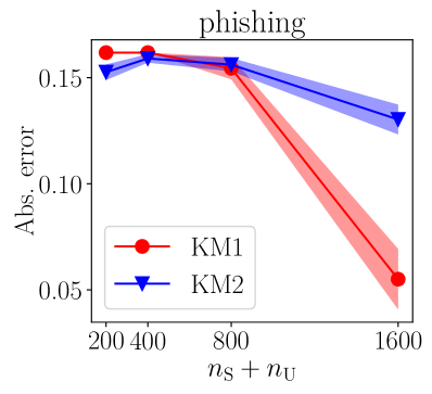
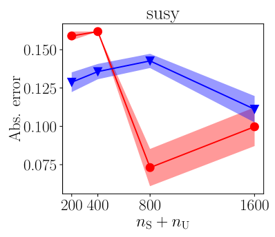
First, we study empirical performance of class-prior estimation. We conduct experiments on benchmark datasets. Different dataset sizes $\{200,400,800,1600\}$ are tested, where half of the data are S pairs and the other half are U data.

In Figure 4, KM1 and KM2 are plotted, which are proposed by Ramaswamy et al. (2016). We used them as CPE in Algorithm 1 . Since $\pi_{\mathrm{S}}=\pi_{+}^{2}+\pi_{-}^{2}=2(\pi_{+}-\frac{1}{2})^{2}+\frac{1}{2}\geq\frac{1}{2}$, we use additional heuristic to set $\lambda_{\mathrm{left}}=2$ in Algorithm 1 of Ramaswamy et al. (2016).

Figure 4: Estimation errors of the class-prior (absolute value of difference between true class-prior and estimated class-prior) from SU data over 100 trials are plotted in the vertical axes. For all experiments, true class-prior $\pi_{+}$ is set to $0.7$.

5.2 Classification Complexity

Figure 5: Average classification error (vertical axes) and standard error (shaded areas) over 50 trials. Different $n_{\mathrm{U}}\in\{200,400,800,1600\}$ are tested, while $n_{\mathrm{S}}$ is fixed to $200$. For each dataset, results with different class-priors ($\pi_{+}\in\{0.1,0.4,0.7\}$) are plotted, which is assumed to be known in advance. Dataset “phoneme” does not have a plot for $\pi_{+}=0.1$ because the number of data in the original dataset is insufficient to subsample SU dataset with $\pi_{+}=0.1$.

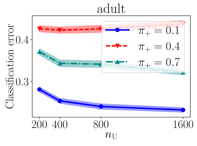
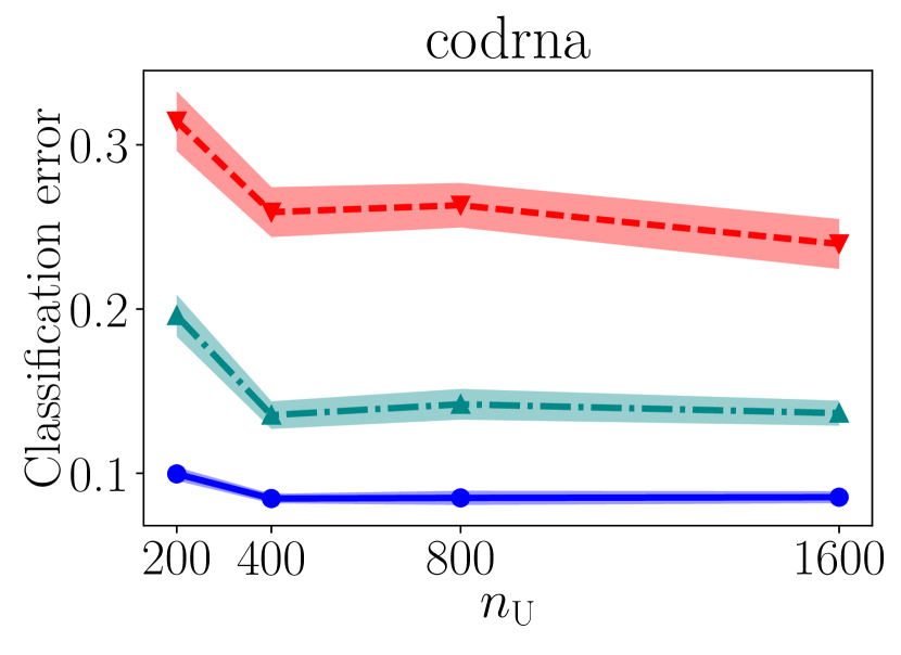
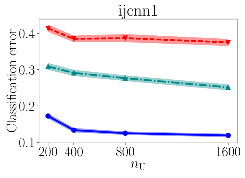
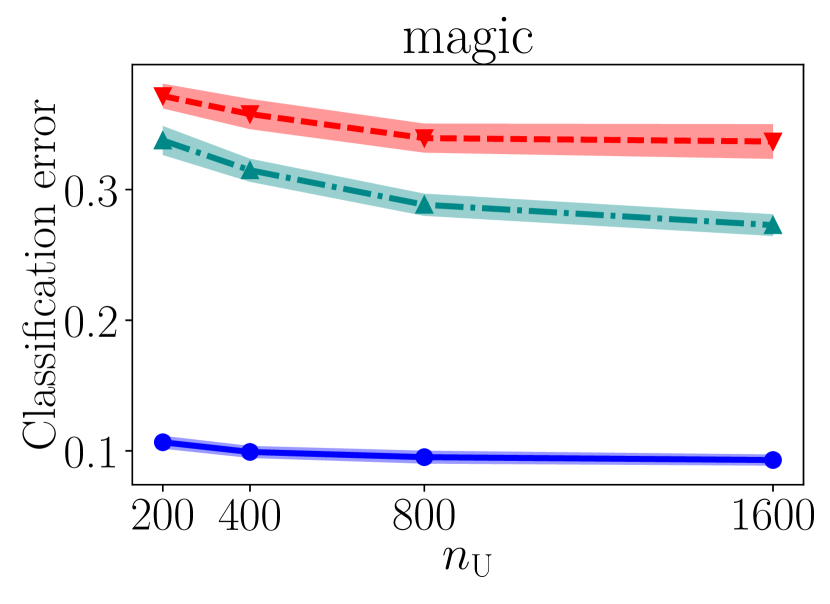
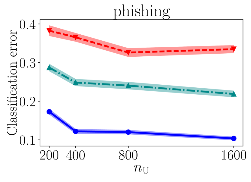
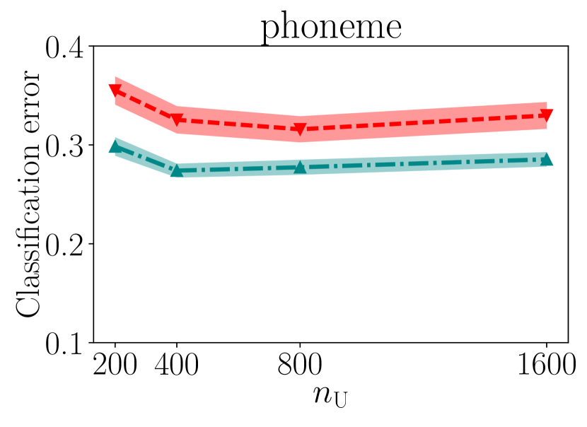
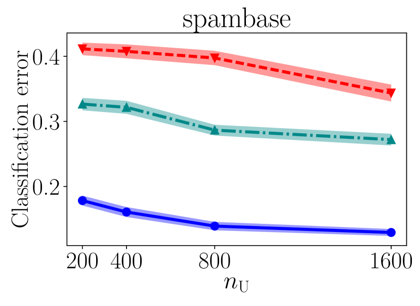
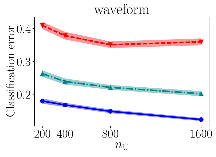
We empirically investigate our proposed method in terms of the relationship between classification performance and the number of training data. We conduct experiments on benchmark datasets with the fixed number of S pairs (fixed to 200), and the different numbers of U data $\{200,400,800,1600\}$.

The experimental results are shown in Figure 5. It indicates that the classification error decreases as $n_{\mathrm{U}}$ grows, which well agree with our theoretical analysis in Theorem 4. Furthermore, we observe a tendency that classification error becomes smaller as the class-prior becomes farther from $\tfrac{1}{2}$. This is because $C_{\mathcal{F},\ell,\delta}$ in Eq. (14) has the term $|2\pi_{+}-1|$ in the denominator, which will make the upper bound looser when $\pi_{+}$ is close to $\tfrac{1}{2}$.

The detailed setting about the proposed method is described below. Our implementation is available at https://github.com/levelfour/SU_Classification.

Proposed Method (SU): We use the linear-in-input model $f(\bm{x})=\bm{w}^{\top}\bm{x}+b$. In Section 5.2, the squared loss is used, and $\pi_{+}$ is given (Case 1 in Table 3). In Section 5.3, the squared loss and the double-hinge loss are used, and the class-prior is estimated by Algorithm 1 with KM2 (Ramaswamy et al., 2016) (Case 2 in Table 3). The regularization parameter $\lambda$ is chosen from $\{10^{-1},10^{-4},10^{-7}\}$.

To choose hyperparameters, 5-fold cross-validation is used. Since we do not have any labeled data in the training phase, the validation error cannot be computed directly. Instead, Eq. (5) equipped with the zero-one loss $\ell_{01}(\cdot)=\frac{1}{2}(1-\mathop{\rm sign}(\cdot))$ is used as a proxy to estimate the validation error. In each experimental trial, the model with minimum validation error is chosen.

5.3 Benchmark Comparison with Baseline Methods

Table 4: Mean accuracy and standard error of SU classification on different benchmark datasets over 20 trials. For all experiments, class-prior $\pi_{+}$ is set to $0.7$. The proposed method does not have oracle $\pi_{+}$ in advance, instead estimating it. Performances are measured by the clustering accuracy $1-\min(r,1-r)$, where $r$ is error rate. Bold-faces indicate outperforming methods, chosen by one-sided t-test with the significance level $5\%$. The result of SERAPH with “w8a” is unavailable due to high-dimensionality and memory constraints.

		SU(proposed)		Baselines
Dataset	Dim	Squared	Double-hinge	KM	ITML	SERAPH	3SMIC	DIMC	IMSAT(linear)
adult	123	64.5 (1.2)	84.5 (0.8)	58.1 (1.1)	57.9 (1.1)	66.5 (1.7)	58.5 (1.3)	63.7 (1.2)	69.8 (0.9)
banana	2	67.5 (1.2)	68.2 (1.2)	54.3 (0.7)	54.8 (0.7)	55.0 (1.1)	61.9 (1.2)	64.3 (1.0)	69.8 (0.9)
cod-rna	8	82.8 (1.3)	71.0 (0.9)	63.1 (1.1)	62.8 (1.0)	62.5 (1.4)	56.6 (1.2)	63.8 (1.1)	69.1 (0.9)
higgs	28	55.1 (1.1)	69.3 (0.9)	66.4 (1.6)	66.6 (1.3)	63.4 (1.1)	57.0 (0.9)	65.0 (1.1)	69.7 (1.4)
ijcnn1	22	65.5 (1.3)	73.6 (0.9)	54.6 (0.9)	55.8 (0.7)	59.8 (1.2)	58.9 (1.3)	66.2 (2.2)	68.5 (1.1)
magic	10	66.0 (2.0)	69.0 (1.3)	53.9 (0.6)	54.5 (0.7)	55.0 (0.9)	59.1 (1.4)	63.1 (1.1)	70.0 (1.1)
phishing	68	75.0 (1.4)	91.3 (0.6)	64.4 (1.0)	61.9 (1.1)	62.4 (1.1)	60.1 (1.3)	64.8 (1.4)	69.4 (0.8)
phoneme	5	67.8 (1.5)	70.8 (1.0)	65.2 (0.9)	66.7 (1.4)	69.1 (1.4)	61.3 (1.1)	64.5 (1.2)	69.2 (1.1)
spambase	57	69.7 (1.4)	85.5 (0.5)	60.1 (1.8)	54.4 (1.1)	65.4 (1.8)	61.5 (1.3)	63.6 (1.3)	70.5 (1.1)
susy	18	59.8 (1.3)	74.8 (1.2)	55.6 (0.7)	55.4 (0.9)	58.0 (1.0)	57.1 (1.2)	65.2 (1.0)	70.4 (1.2)
w8a	300	62.1 (1.5)	86.5 (0.6)	71.0 (0.8)	69.5 (1.5)	0.0 (0.0)	60.5 (1.5)	65.0 (2.0)	70.2 (1.2)
waveform	21	77.8 (1.3)	87.0 (0.5)	56.1 (0.8)	54.8 (0.7)	56.5 (0.9)	56.5 (0.9)	65.0 (0.9)	69.7 (1.1)

We compare our proposed method with baseline methods on benchmark datasets. We conduct experiments on each dataset with 500 similar data pairs, 500 unlabeled data, and 100 test data. As can be seen from Table 4, our proposed method outperforms baselines for many datasets. The details about the baseline methods are described below.

Baseline 1 (KM): As a simple baseline, we consider $k$-means clustering (MacQueen, 1967). We ignore pair information of S data and apply $k$-means clustering with $k=2$ to U data.

Baseline 2 (ITML): Information-theoretic metric learning (Davis et al., 2007) is a metric learning method by regularizing the covariance matrix based on prior knowledge, with pairwise constraints. We use the identity matrix as prior knowledge, and the slack variable parameter is fixed to $\gamma=1$, since we cannot employ the cross-validation without any class label information. Using the obtained metric, $k$-means clustering is applied on test data.

Baseline 3 (SERAPH): Semi-supervised metric learning paradigm with hyper sparsity (Niu et al., 2012) is another metric learning method based on entropy regularization. Hyperparameter choice follows $\textsc{Seraph}_{\mathrm{hyper}}$. Using the obtained metric, $k$-means clustering is applied on test data.

Baseline 4 (3SMIC): Semi-supervised SMI-based clustering (Calandriello et al., 2014) models class-posteriors and maximizes mutual information between unlabeled data at hand and their cluster labels. The penalty parameter $\gamma$ and the kernel parameter $t$ are chosen from $\{10^{-2},10^{0},10^{2}\}$ and $\{4,7,10\}$, respectively, via 5-fold cross-validation.

Baseline 5 (DIMC): DirtyIMC (Chiang et al., 2015) is a noisy version of inductive matrix completion, where the similarity matrix is recovered from a low-rank feature matrix. Similarity matrix $S$ is assumed to be expressed as $UU^{\top}$, where $U$ is low-rank feature representations of input data. After obtaining $U$, $k$-means clustering is conducted on $U$. Two hyperparameters $\lambda_{M},\lambda_{N}$ in Eq. (2) in (Chiang et al., 2015) are set to $\lambda_{M}=\lambda_{N}=10^{-2}$.

Baseline 6 (IMSAT): Information maximizing self-augmented training (Hu et al., 2017) is an unsupervised learning method to make a probabilistic classifier that maps similar data to similar representations, combining information maximization clustering with self-augmented training, which make the predictions of perturbed data close to the predictions of the original ones. Instead of data perturbation, self-augmented training can be applied on S data to make each pair of data similar. Here the logistic regressor $p_{\bm{\theta}}(y|\bm{x})=(1+\exp(-\bm{\theta}^{\top}\bm{x}))^{-1}$ is used as a classification model, where $\bm{\theta}$ is parameters to learn. Trade-off parameter $\lambda$ is set to $1$.

Remark: KM, ITML, and SERAPH rely on $k$-means, which is trained by using only training data. Test prediction is based on the metric between test data and learned cluster centers. Among the baselines, DIMC can only handle in-sample prediction, so it is trained by using both training and test data at the same time.

6 Conclusion

In this paper, we proposed a novel weakly-supervised learning problem named SU classification, where only similar pairs and unlabeled data are needed. SU classification even becomes class-identifiable under a certain condition on the class-prior (see Table 3). Its optimization problem with the linear-in-parameter model becomes convex if we choose certain loss functions such as the squared loss and the double-hinge loss. We established an estimation error bound for the proposed method, and confirmed that the estimation error decreases with the parametric optimal order, as the number of similar data and unlabeled data becomes larger. We also investigated the empirical performance and confirmed that our proposed method performs better than baseline methods.

Appendix A Proof of Lemma 1

From the assumption (2), $\mathcal{D}_{\mathrm{S}}=\{(\bm{x}_{\mathrm{S},i},\bm{x}_{\mathrm{S},i}^{\prime})\}_{i=1}^{n_{\mathrm{S}}}\sim p_{\mathrm{S}}(\bm{x},\bm{x}^{\prime})$. In order to decompose pairwise data into pointwise, marginalize $p_{\mathrm{S}}(\bm{x},\bm{x}^{\prime})$ with respect to $\bm{x}^{\prime}$:

$$\int p_{\mathrm{S}}(\bm{x},\bm{x}^{\prime})d\bm{x}^{\prime} =\frac{\pi_{+}^{2}}{\pi_{+}^{2}+\pi_{-}^{2}}p_{+}(\bm{x})\int p_{+}(\bm{x}^{\prime})d\bm{x}^{\prime}+\frac{\pi_{-}^{2}}{\pi_{+}^{2}+\pi_{-}^{2}}p_{-}(\bm{x})\int p_{-}(\bm{x}^{\prime})d\bm{x}^{\prime}$$

$$=\frac{\pi_{+}^{2}}{\pi_{+}^{2}+\pi_{-}^{2}}p_{+}(\bm{x})\int\frac{p(\bm{x}^{\prime},y=+1)}{p(y=+1)}d\bm{x}^{\prime}+\frac{\pi_{-}^{2}}{\pi_{+}^{2}+\pi_{-}^{2}}p_{-}(\bm{x})\int\frac{p(\bm{x}^{\prime},y=-1)}{p(y=-1)}d\bm{x}^{\prime}$$

$$=\frac{\pi_{+}^{2}}{\pi_{+}^{2}+\pi_{-}^{2}}p_{+}(\bm{x})\frac{p(y=+1)}{p(y=+1)}+\frac{\pi_{-}^{2}}{\pi_{+}^{2}+\pi_{-}^{2}}p_{-}(\bm{x})\frac{p(y=-1)}{p(y=-1)}$$

$$=\frac{\pi_{+}^{2}}{\pi_{+}^{2}+\pi_{-}^{2}}p_{+}(\bm{x})+\frac{\pi_{-}^{2}}{\pi_{+}^{2}+\pi_{-}^{2}}p_{-}(\bm{x})$$

$$=\widetilde{p}_{\mathrm{S}}(\bm{x}).$$

Since a pair $(\bm{x}_{\mathrm{S},i},\bm{x}_{\mathrm{S},i}^{\prime})\in\mathcal{D}_{\mathrm{S}}$ is independently and identically drawn, both $\bm{x}_{\mathrm{S},i}$ and $\bm{x}_{\mathrm{S},i}^{\prime}$ are drawn following $\widetilde{p}_{\mathrm{S}}$. ∎

Appendix B Proof of Theorem 1

To prove Theorem 1, it is convenient to begin with the following Lemma 3.

Lemma 3.

The classification risk (1) can be equivalently expressed as

$$R {}_{\mathrm{PSD},\ell}(f)=\frac{\pi_{+}}{2\pi_{-}}\mathop{\mathbb{E}}_{X\sim p_{+}}\left[\widetilde{\ell}(f(X))\right]$$

$$+\pi_{\mathrm{S}}\mathop{\mathbb{E}}_{(X,X^{\prime})\sim p_{\mathrm{S}}}\left[-\frac{\pi_{+}}{2\pi_{-}}\frac{\ell(f(X),+1)+\ell(f(X^{\prime}),+1)}{2}+\frac{1+\pi_{-}}{2\pi_{-}}\frac{\ell(f(X),-1)+\ell(f(X^{\prime}),-1)}{2}\right]$$

$$+\pi_{\mathrm{D}}\mathop{\mathbb{E}}_{(X,X^{\prime})\sim p_{\mathrm{D}}}\left[\frac{\ell(f(X),-1)+\ell(f(X^{\prime}),+1)}{2}\right],$$ (B.1)

where $\mathbb{E}_{X\sim p_{+}}[\cdot]$, $\mathbb{E}_{(X,X^{\prime})\sim p_{\mathrm{S}}}[\cdot]$, and $\mathbb{E}_{(X,X^{\prime})\sim p_{\mathrm{D}}}[\cdot]$ denote expectations over $p_{+}(X)$, $p_{\mathrm{S}}(X,X^{\prime})$, and $p_{\mathrm{D}}(X,X^{\prime})$, respectively.

Note that the definitions of $p_{\mathrm{D}}$ and $\pi_{\mathrm{D}}$ are first given in Eq. (12).

Proof.

Eq. (1) can be transformed into pairwise fashion:

$$\mathop{\mathbb{E}}_{(X,Y)\sim p}[\ell(f(X),Y)] =\mathop{\mathbb{E}}_{(X,Y)\sim p}\left[\frac{\ell(f(X),Y)}{2}\right]+\mathop{\mathbb{E}}_{(X^{\prime},Y^{\prime})\sim p}\left[\frac{\ell(f(X^{\prime}),Y^{\prime})}{2}\right]$$

$$=\mathop{\mathbb{E}}_{(X,Y),(X^{\prime},Y^{\prime})\sim p}\left[\frac{\ell(f(X),Y)+\ell(f(X^{\prime}),Y^{\prime})}{2}\right].$$ (B.2)

Both pairs $(X,Y)$ and $(X^{\prime},Y^{\prime})$ are independently and identically distributed from the joint distribution $p(\bm{x},y)$. Thus, Eq. (B.2) can be further decomposed:

$$\mathop{\mathbb{E}}_{(X,Y),(X^{\prime},Y^{\prime})\sim p} \left[\frac{\ell(f(X),Y)+\ell(f(X^{\prime}),Y^{\prime})}{2}\right]$$

$$=\sum_{y,y^{\prime}}\int\frac{\ell(f(\bm{x}),y)+\ell(f(\bm{x}^{\prime}),y^{\prime})}{2}p(\bm{x},y)p(\bm{x}^{\prime},y^{\prime})d\bm{x}d\bm{x}^{\prime}$$

$$=\pi_{+}^{2}\int\frac{\ell(f(\bm{x}),+1)+\ell(f(\bm{x}^{\prime}),+1)}{2}p_{+}(\bm{x})p_{+}(\bm{x}^{\prime})d\bm{x}d\bm{x}^{\prime}$$

$$\quad+\pi_{-}^{2}\int\frac{\ell(f(\bm{x}),-1)+\ell(f(\bm{x}^{\prime}),-1)}{2}p_{-}(\bm{x})p_{-}(\bm{x}^{\prime})d\bm{x}d\bm{x}^{\prime}$$

$$\quad+\pi_{+}\pi_{-}\int\frac{\ell(f(\bm{x}),+1)+\ell(f(\bm{x}^{\prime}),-1)}{2}p_{+}(\bm{x})p_{-}(\bm{x}^{\prime})d\bm{x}d\bm{x}^{\prime}$$

$$\quad+\pi_{+}\pi_{-}\int\frac{\ell(f(\bm{x}),-1)+\ell(f(\bm{x}^{\prime}),+1)}{2}p_{-}(\bm{x})p_{+}(\bm{x}^{\prime})d\bm{x}d\bm{x}^{\prime}$$

$$=\pi_{+}^{2}\mathop{\mathbb{E}}_{X,X^{\prime}\sim p_{+}}\left[\frac{\ell(f(X),+1)+\ell(f(X^{\prime}),+1)}{2}\right]$$

$$\qquad+\pi_{-}^{2}\mathop{\mathbb{E}}_{X,X^{\prime}\sim p_{-}}\left[\frac{\ell(f(X),-1)+\ell(f(X^{\prime}),-1)}{2}\right]$$

$$\qquad+\pi_{+}\pi_{-}\mathop{\mathbb{E}}_{X\sim p_{+},X^{\prime}\sim p_{-}}\left[\frac{\ell(f(X),+1)+\ell(f(X^{\prime}),-1)}{2}\right]$$

$$\qquad+\pi_{+}\pi_{-}\mathop{\mathbb{E}}_{X\sim p_{-},X^{\prime}\sim p_{+}}\left[\frac{\ell(f(X),-1)+\ell(f(X^{\prime}),+1)}{2}\right].$$ (B.3)

Using Eq. (2), the following equation is obtained:

$$\pi_{\mathrm{S}} \mathop{\mathbb{E}}_{(X,X^{\prime})\sim p_{\mathrm{S}}}\left[\frac{\ell(f(X),-1)+\ell(f(X^{\prime}),-1)}{2}\right]$$

$$=\pi_{+}^{2}\mathop{\mathbb{E}}_{X,X^{\prime}\sim p_{+}}\left[\frac{\ell(f(X),-1)+\ell(f(X^{\prime}),-1)}{2}\right]+\pi_{-}^{2}\mathop{\mathbb{E}}_{X,X^{\prime}\sim p_{-}}\left[\frac{\ell(f(X),-1)+\ell(f(X^{\prime}),-1)}{2}\right].$$ (B.4)

Similarly, the following equation is obtained from Eq. (12):

$$2 \pi_{-}\pi_{+}\mathop{\mathbb{E}}_{(X,X^{\prime})\sim p_{\mathrm{D}}}\left[\frac{\ell(f(X),-1)+\ell(f(X^{\prime}),+1)}{2}\right]$$

$$=\pi_{+}\pi_{-}\mathop{\mathbb{E}}_{X\sim p_{+},X^{\prime}\sim p_{-}}\left[\frac{\ell(f(X),-1)+\ell(f(X^{\prime}),+1)}{2}\right]+\pi_{+}\pi_{-}\mathop{\mathbb{E}}_{X\sim p_{-},X\sim p_{+}}\left[\frac{\ell(f(X),-1)+\ell(f(X^{\prime}),+1)}{2}\right].$$ (B.5)

Combining Eqs. (B.3), (B.4) and (B.5), the expected risk $R(f)$ is written as

$$R(f) =\pi_{\mathrm{S}}\mathop{\mathbb{E}}_{(X,X^{\prime})\sim p_{\mathrm{S}}}\left[\frac{\ell(f(X),-1)+\ell(f(X^{\prime}),-1)}{2}\right]+\pi_{\mathrm{D}}\mathop{\mathbb{E}}_{(X,X^{\prime})\sim p_{\mathrm{D}}}\left[\frac{\ell(f(X),-1)+\ell(f(X^{\prime}),+1)}{2}\right]$$

$$\quad+\pi_{+}^{2}\mathop{\mathbb{E}}_{X,X^{\prime}\sim p_{+}}\left[\frac{\widetilde{\ell}(f(X))+\widetilde{\ell}(f(X^{\prime}))}{2}\right]+\pi_{+}\pi_{-}\mathop{\mathbb{E}}_{X\sim p_{+},X^{\prime}\sim p_{-}}\left[\frac{\widetilde{\ell}(f(X))-\widetilde{\ell}(f(X^{\prime}))}{2}\right].$$ (B.6)

Here

• the second term on the RHS of Eq. (B.4) is substituted into the second term in the last line of Eq. (B.3).

• the second term on the RHS of Eq. (B.5) is substituted into the fourth term in the last line of Eq. (B.3).

On the third and fourth term on the RHS of Eq. (B.6),

$$\pi_{+}^{2} \mathop{\mathbb{E}}_{X,X^{\prime}\sim p_{+}}\left[\frac{\widetilde{\ell}(f(X))+\widetilde{\ell}(f(X^{\prime}))}{2}\right]+\pi_{+}\pi_{-}\mathop{\mathbb{E}}_{X\sim p_{+},X^{\prime}\sim p_{-}}\left[\frac{\widetilde{\ell}(f(X))-\widetilde{\ell}(f(X^{\prime}))}{2}\right]$$

$$=\pi_{+}^{2}\left\{\frac{1}{2}\mathop{\mathbb{E}}_{X\sim p_{+}}\left[\widetilde{\ell}(f(X))\right]+\frac{1}{2}\mathop{\mathbb{E}}_{X^{\prime}\sim p_{+}}\left[\widetilde{\ell}(f(X^{\prime}))\right]\right\}+\pi_{+}\pi_{-}\left\{\frac{1}{2}\mathop{\mathbb{E}}_{X\sim p_{+}}\left[\widetilde{\ell}(f(X))\right]-\frac{1}{2}\mathop{\mathbb{E}}_{X^{\prime}\sim p_{-}}\left[\widetilde{\ell}(f(X^{\prime}))\right]\right\}$$

$$=\pi_{+}^{2}\mathop{\mathbb{E}}_{X\sim p_{+}}\left[\widetilde{\ell}(f(X))\right]+\frac{1}{2}\pi_{+}\pi_{-}\mathop{\mathbb{E}}_{X\sim p_{+}}\left[\widetilde{\ell}(f(X))\right]-\frac{1}{2}\pi_{+}\pi_{-}\mathop{\mathbb{E}}_{X\sim p_{-}}\left[\widetilde{\ell}(f(X))\right]$$

$$=\frac{\pi_{+}(1+\pi_{+})}{2}\mathop{\mathbb{E}}_{X\sim p_{+}}\left[\widetilde{\ell}(f(X))\right]-\frac{\pi_{+}(1-\pi_{+})}{2}\mathop{\mathbb{E}}_{X\sim p_{-}}\left[\widetilde{\ell}(f(X))\right]$$

$$=(\ast).$$ (B.7)

Here similarly to derivation of Eq. (B.4),

$$\pi_{\mathrm{S}} \mathop{\mathbb{E}}_{(X,X^{\prime})\sim p_{\mathrm{S}}}\left[\frac{\widetilde{\ell}(f(X))+\widetilde{\ell}(f(X^{\prime}))}{2}\right]$$

$$=\pi_{+}^{2}\mathop{\mathbb{E}}_{X,X^{\prime}\sim p_{+}}\left[\frac{\widetilde{\ell}(f(X))+\widetilde{\ell}(f(X^{\prime}))}{2}\right]+\pi_{-}^{2}\mathop{\mathbb{E}}_{X,X^{\prime}\sim p_{-}}\left[\frac{\widetilde{\ell}(f(X))+\widetilde{\ell}(f(X^{\prime}))}{2}\right]$$

$$=\pi_{+}^{2}\mathop{\mathbb{E}}_{X\sim p_{+}}\left[\widetilde{\ell}(f(X))\right]+\pi_{-}^{2}\mathop{\mathbb{E}}_{X\sim p_{-}}\left[\widetilde{\ell}(f(X))\right].$$ (B.8)

Combining Eqs. (B.7) and (B.8),

$$(\ast) =\frac{\pi_{+}(1+\pi_{+})}{2}\mathop{\mathbb{E}}_{X\sim p_{+}}\left[\widetilde{\ell}(f(X))\right]-\frac{\pi_{+}(1-\pi_{+})}{2\pi_{-}^{2}}\left\{-\pi_{+}^{2}\mathop{\mathbb{E}}_{X\sim p_{+}}\left[\widetilde{\ell}(f(X))\right]+\pi_{\mathrm{S}}\mathop{\mathbb{E}}_{(X,X^{\prime})\sim p_{\mathrm{S}}}\left[\frac{\widetilde{\ell}(f(X))+\widetilde{\ell}(f(X^{\prime}))}{2}\right]\right\}$$

$$=\frac{\pi_{+}}{2\pi_{-}}\mathop{\mathbb{E}}_{X\sim p_{+}}\left[\widetilde{\ell}(f(X))\right]-\frac{\pi_{+}\pi_{\mathrm{S}}}{2\pi_{-}}\mathop{\mathbb{E}}_{(X,X^{\prime})\sim p_{\mathrm{S}}}\left[\frac{\widetilde{\ell}(f(X))+\widetilde{\ell}(f(X^{\prime}))}{2}\right].$$ (B.9)

Finally from Eqs. (B.6) and (B.9), the expected risk $R(f)$ is written as

$$R(f) =\pi_{\mathrm{S}}\mathop{\mathbb{E}}_{(X,X^{\prime})\sim p_{\mathrm{S}}}\left[\frac{\ell(f(X),-1)+\ell(f(X^{\prime}),-1)}{2}\right]+\pi_{\mathrm{D}}\mathop{\mathbb{E}}_{(X,X^{\prime})\sim p_{\mathrm{D}}}\left[\frac{\ell(f(X),-1)+\ell(f(X^{\prime}),+1)}{2}\right]$$

$$\quad+\frac{\pi_{+}}{2\pi_{-}}\mathop{\mathbb{E}}_{X\sim p_{+}}\left[\widetilde{\ell}(f(X))\right]-\frac{\pi_{+}\pi_{\mathrm{S}}}{2\pi_{-}}\mathop{\mathbb{E}}_{(X,X^{\prime})\sim p_{\mathrm{S}}}\left[\frac{\widetilde{\ell}(f(X))+\widetilde{\ell}(f(X^{\prime}))}{2}\right]$$

$$=R_{\mathrm{PSD},\ell}(f).$$ (B.10)

∎

Now we give a proof for Theorem 1.

Proof of Theorem 1.

By Lemma 3, it is enough to show $R_{\mathrm{SU},\ell}(f)=R_{\mathrm{PSD},\ell}(f)$.

From Eq. (11),

$$\mathop{\mathbb{E}}_{X\sim p} \left[\frac{\ell(f(X),-1)+\ell(f(X),+1)}{2}\right]$$

$$=\mathop{\mathbb{E}}_{X\sim p}\left[\frac{\ell(f(X),-1)}{2}\right]+\mathop{\mathbb{E}}_{X\sim p}\left[\frac{\ell(f(X)),+1}{2}\right]\qquad\qquad\text{($\because$ linearity of the expectation)}$$

$$=\mathop{\mathbb{E}}_{X\sim p}\left[\frac{\ell(f(X),-1)}{2}\right]+\mathop{\mathbb{E}}_{X^{\prime}\sim p}\left[\frac{\ell(f(X^{\prime})),+1}{2}\right]$$

$$=\mathop{\mathbb{E}}_{X,X^{\prime}\sim p}\left[\frac{\ell(f(X),-1)+\ell(f(X^{\prime}),+1)}{2}\right]$$

$$=\pi_{\mathrm{S}}\mathop{\mathbb{E}}_{(X,X^{\prime})\sim p_{\mathrm{S}}}\left[\frac{\ell(f(X),-1)+\ell(f(X^{\prime}),+1)}{2}\right]+\pi_{\mathrm{D}}\mathop{\mathbb{E}}_{(X,X^{\prime})\sim p_{\mathrm{D}}}\left[\frac{\ell(f(X),-1)+\ell(f(X^{\prime}),+1)}{2}\right],$$ (B.11)

where $\mathbb{E}_{X\sim p}[\cdot]$ denotes the expectation over the marginal distribution $p(X)$ and the last equality is obtained from Eq. (11). Eq. (B.11) produces an alternative expression of the expectation over $p_{\mathrm{D}}$ (the third term on the RHS of Eq. (B.1)):

$$\pi_{\mathrm{D}} \mathop{\mathbb{E}}_{(X,X^{\prime})\sim p_{\mathrm{D}}}\left[\frac{\ell(f(X),-1)+\ell(f(X^{\prime}),+1)}{2}\right]$$

$$=\mathop{\mathbb{E}}_{X\sim p}\left[\frac{\ell(f(X),-1)+\ell(f(X),+1)}{2}\right]-\pi_{\mathrm{S}}\mathop{\mathbb{E}}_{(X,X^{\prime})\sim p_{\mathrm{S}}}\left[\frac{\ell(f(X),-1)+\ell(f(X^{\prime}),+1)}{2}\right].$$ (B.12)

Next, we obtain an alternative expression of the expectation over positive data (the first term in RHS of Eq. (B.1)). The following two equations (B.13) and (B.14) are useful:

$$\mathop{\mathbb{E}}_{X\sim p} \left[\widetilde{\ell}(f(X))\right]=\pi_{+}\mathop{\mathbb{E}}_{X\sim p_{+}}\left[\widetilde{\ell}(f(X))\right]+\pi_{-}\mathop{\mathbb{E}}_{X\sim p_{-}}\left[\widetilde{\ell}(f(X))\right],$$ (B.13)

which can simply be obtained from Eq. (3).

$$\pi_{\mathrm{S}}\mathop{\mathbb{E}}_{(X,X^{\prime})\sim p_{\mathrm{S}}}\left[\frac{\widetilde{\ell}(f(X))+\widetilde{\ell}(f(X^{\prime}))}{2}\right] =\pi_{+}^{2}\mathop{\mathbb{E}}_{X,X^{\prime}\sim p_{+}}\left[\frac{\widetilde{\ell}(f(X))+\widetilde{\ell}(f(X^{\prime}))}{2}\right]+\pi_{-}^{2}\mathop{\mathbb{E}}_{X,X^{\prime}\sim p_{-}}\left[\frac{\widetilde{\ell}(f(X))+\widetilde{\ell}(f(X^{\prime}))}{2}\right]$$

$$=\pi_{+}^{2}\left\{\frac{1}{2}\mathop{\mathbb{E}}_{X\sim p_{+}}\left[\widetilde{\ell}(f(X))\right]+\frac{1}{2}\mathop{\mathbb{E}}_{X^{\prime}\sim p_{+}}\left[\widetilde{\ell}(f(X^{\prime}))\right]\right\}$$

$$\qquad+\pi_{-}^{2}\left\{\frac{1}{2}\mathop{\mathbb{E}}_{X\sim p_{-}}\left[\widetilde{\ell}(f(X))\right]+\frac{1}{2}\mathop{\mathbb{E}}_{X^{\prime}\sim p_{-}}\left[\widetilde{\ell}(f(X^{\prime}))\right]\right\}$$

$$=\pi_{+}^{2}\mathop{\mathbb{E}}_{X\sim p_{+}}\left[\widetilde{\ell}(f(X))\right]+\pi_{-}^{2}\mathop{\mathbb{E}}_{X\sim p_{-}}\left[\widetilde{\ell}(f(X))\right],$$ (B.14)

which is obtained from Eq. (2). By calculating $\text{\eqref{eq:expectation-of-positive-alt-sub2}}-\pi_{-}\times\text{\eqref{eq:expectation-of-positive-alt-sub1}}$ and organizing, we obtain

$$\frac{\pi_{+}}{2\pi_{-}} \mathop{\mathbb{E}}_{X\sim p_{+}}\left[\widetilde{\ell}(f(X))\right]=\frac{\pi_{\mathrm{S}}}{2\pi_{-}(2\pi_{+}-1)}\mathop{\mathbb{E}}_{(X,X^{\prime})\sim p_{\mathrm{S}}}\left[\frac{\widetilde{\ell}(f(X))+\widetilde{\ell}(f(X^{\prime}))}{2}\right]-\frac{1}{2(2\pi_{+}-1)}\mathop{\mathbb{E}}_{X\sim p}\left[\widetilde{\ell}(f(X))\right].$$ (B.15)

Substituting Eqs. (B.12) and (B.15) into Eq. (B.1),

$$R_{\mathrm{PSD},\ell}(f) =\frac{\pi_{\mathrm{S}}}{2\pi_{-}(2\pi_{+}-1)}\mathop{\mathbb{E}}_{(X,X^{\prime})\sim p_{\mathrm{S}}}\left[\frac{\widetilde{\ell}(f(X))+\widetilde{\ell}(f(X^{\prime}))}{2}\right]-\frac{1}{2(2\pi_{+}-1)}\mathop{\mathbb{E}}_{X\sim p}\left[\widetilde{\ell}(f(X))\right]$$

$$\quad+\pi_{\mathrm{S}}\mathop{\mathbb{E}}_{(X,X^{\prime})\sim p_{\mathrm{S}}}\left[-\frac{\pi_{+}}{2\pi_{-}}\frac{\ell(f(X),+1)+\ell(f(X^{\prime}),+1)}{2}+\frac{1+\pi_{-}}{2\pi_{-}}\frac{\ell(f(X),-1)+\ell(f(X^{\prime}),-1)}{2}\right]$$

$$\quad+\mathop{\mathbb{E}}_{X\sim p}\left[\frac{\ell(f(X),-1)+\ell(f(X),+1)}{2}\right]-\pi_{\mathrm{S}}\mathop{\mathbb{E}}_{(X,X^{\prime})\sim p_{\mathrm{S}}}\left[\frac{\ell(f(X),-1)+\ell(f(X^{\prime}),+1)}{2}\right]$$

$$=\pi_{\mathrm{S}}\mathop{\mathbb{E}}_{(X,X^{\prime})\sim p_{\mathrm{S}}}\left[\frac{1+2\pi_{+}}{4(2\pi_{+}-1)}\widetilde{\ell}(f(X))+\frac{1+2\pi_{-}}{4(2\pi_{+}-1)}\widetilde{\ell}(f(X^{\prime}))\right]$$

$$\quad+\mathop{\mathbb{E}}_{X\sim p}\left[-\frac{\pi_{-}}{2\pi_{+}-1}\ell(f(X),+1)+\frac{\pi_{+}}{2\pi_{+}-1}\ell(f(X),-1)\right]$$

$$=\pi_{\mathrm{S}}\mathop{\mathbb{E}}_{(X,X^{\prime})\sim p_{\mathrm{S}}}\left[\frac{\frac{1}{2\pi_{+}-1}\widetilde{\ell}(f(X))+\frac{1}{2\pi_{+}-1}\widetilde{\ell}(f(X^{\prime}))}{2}\right]$$

$$\qquad+\mathop{\mathbb{E}}_{X\sim p}\left[-\frac{\pi_{-}}{2\pi_{+}-1}\ell(f(X),+1)+\frac{\pi_{+}}{2\pi_{+}-1}\ell(f(X),-1)\right]$$ (B.16)

$$=R_{\mathrm{SU},\ell}(f),$$

which concludes the proof. The third equality of Eq. (B.16) holds because $X$ and $X^{\prime}$ are symmetric and

$$\frac{1+2\pi_{+}}{4(2\pi_{+}-1)}\widetilde{\ell}(\cdot)+\frac{1+2\pi_{-}}{4(2\pi_{+}-1)}\widetilde{\ell}(\cdot)=\frac{1}{2\pi_{+}-1}\widetilde{\ell}(\cdot)=\frac{\frac{1}{2\pi_{+}-1}\widetilde{\ell}(\cdot)+\frac{1}{2\pi_{+}-1}\widetilde{\ell}(\cdot)}{2}.$$

∎

Appendix C Discussion on Variance of Risk Estimator

C.1 Proof of Lemma 2

The statement can be simply confirmed as follows:

$$\mathop{\mathbb{E}}_{(X,X^{\prime})\sim p_{\mathrm{S}}}\left[\frac{\mathcal{L}_{\mathrm{S},\ell}(f(X))+\mathcal{L}_{\mathrm{S},\ell}(f(X^{\prime}))}{2}\right] =\mathop{\mathbb{E}}_{X\sim\widetilde{p}_{\mathrm{S}}}\left[\frac{\mathcal{L}_{\mathrm{S},\ell}(f(X))}{2}\right]+\mathop{\mathbb{E}}_{X^{\prime}\sim\widetilde{p}_{\mathrm{S}}}\left[\frac{\mathcal{L}_{\mathrm{S},\ell}(f(X^{\prime}))}{2}\right]$$

$$=\mathop{\mathbb{E}}_{X\sim\widetilde{p}_{\mathrm{S}}}\left[\mathcal{L}_{\mathrm{S},\ell}(f(X))\right]$$

$$=\mathop{\mathbb{E}}_{X\sim\widetilde{p}_{\mathrm{S}}}\left[\alpha\mathcal{L}_{\mathrm{S},\ell}(f(X))+(1-\alpha)\mathcal{L}_{\mathrm{S},\ell}(f(X))\right]$$

$$=\mathop{\mathbb{E}}_{X\sim\widetilde{p}_{\mathrm{S}}}\left[\alpha\mathcal{L}_{\mathrm{S},\ell}(f(X))\right]+\mathop{\mathbb{E}}_{X^{\prime}\sim\widetilde{p}_{\mathrm{S}}}\left[(1-\alpha)\mathcal{L}_{\mathrm{S},\ell}(f(X^{\prime}))\right]$$

$$=\mathop{\mathbb{E}}_{(X,X^{\prime})\sim p_{\mathrm{S}}}\left[\alpha\mathcal{L}_{\mathrm{S},\ell}(f(X))+(1-\alpha)\mathcal{L}_{\mathrm{S},\ell}(f(X^{\prime}))\right].$$

∎

C.2 Proof of Theorem 2

We show Eq. (8) is the variance minimizer of

$$S(f;\alpha)\triangleq\frac{1}{n_{\mathrm{S}}}\sum_{i=1}^{n_{\mathrm{S}}}\left\{\alpha\mathcal{L}_{\mathrm{S},\ell}(f(\bm{x}_{\mathrm{S},i}))+(1-\alpha)\mathcal{L}_{\mathrm{S},\ell}(f(\bm{x}_{\mathrm{S},i}^{\prime}))\right\},$$

with respect to $\alpha\in\mathbb{R}$. Let $\mu_{1}\triangleq\mathop{\mathbb{E}}_{\{(\bm{x}_{\mathrm{S},i},\bm{x}_{\mathrm{S},i}^{\prime})\}\sim p_{\mathrm{S}}}[S(f;\alpha)]$ and

$$\widetilde{\mu}_{1} \triangleq\mathop{\mathbb{E}}_{\{\bm{x}_{\mathrm{S},i}\}\sim\widetilde{p}_{\mathrm{S}}}\left[\frac{1}{n_{\mathrm{S}}}\sum_{i=1}^{n_{\mathrm{S}}}\mathcal{L}_{\mathrm{S},\ell}(f(\bm{x}_{\mathrm{S},i}))\right]=\mathop{\mathbb{E}}_{\{\bm{x}_{\mathrm{S},i}^{\prime}\}\sim\widetilde{p}_{\mathrm{S}}}\left[\frac{1}{n_{\mathrm{S}}}\sum_{i=1}^{n_{\mathrm{S}}}\mathcal{L}_{\mathrm{S},\ell}(f(\bm{x}_{\mathrm{S},i}^{\prime}))\right],$$

$$\widetilde{\mu}_{2} \triangleq\mathop{\mathbb{E}}_{\{\bm{x}_{\mathrm{S},i}\}\sim\widetilde{p}_{\mathrm{S}}}\left[\left(\frac{1}{n_{\mathrm{S}}}\sum_{i=1}^{n_{\mathrm{S}}}\mathcal{L}_{\mathrm{S},\ell}(f(\bm{x}_{\mathrm{S},i}))\right)^{2}\right]=\mathop{\mathbb{E}}_{\{\bm{x}_{\mathrm{S},i}^{\prime}\}\sim\widetilde{p}_{\mathrm{S}}}\left[\left(\frac{1}{n_{\mathrm{S}}}\sum_{i=1}^{n_{\mathrm{S}}}\mathcal{L}_{\mathrm{S},\ell}(f(\bm{x}_{\mathrm{S},i}^{\prime}))\right)^{2}\right].$$

Then,

$$\mathrm{Var}(S(f;\alpha)) =\mathop{\mathbb{E}}_{\{(\bm{x}_{\mathrm{S},i},\bm{x}_{\mathrm{S},i}^{\prime})\}\sim p_{\mathrm{S}}}\left[\left(S(f;\alpha)-\mu_{1}\right)^{2}\right]$$

$$=\mathop{\mathbb{E}}_{\{(\bm{x}_{\mathrm{S},i},\bm{x}_{\mathrm{S},i}^{\prime})\}\sim p_{\mathrm{S}}}\left[S(f;\alpha)^{2}\right]-\mu_{1}^{2}$$

$$=\alpha^{2}\mathop{\mathbb{E}}_{\{\bm{x}_{\mathrm{S},i}\}\sim\widetilde{p}_{\mathrm{S}}}\left[\left(\frac{1}{n_{\mathrm{S}}}\sum_{i=1}^{n_{\mathrm{S}}}\mathcal{L}_{\mathrm{S},\ell}(f(\bm{x}_{\mathrm{S},i}))\right)^{2}\right]$$

$$\qquad+2\alpha(1-\alpha)\mathop{\mathbb{E}}_{\{\bm{x}_{\mathrm{S},i}\}\sim\widetilde{p}_{\mathrm{S}}}\left[\frac{1}{n_{\mathrm{S}}}\sum_{i=1}^{n_{\mathrm{S}}}\mathcal{L}_{\mathrm{S},\ell}(f(\bm{x}_{\mathrm{S},i}))\right]\mathop{\mathbb{E}}_{\{\bm{x}_{\mathrm{S},i}^{\prime}\}\sim\widetilde{p}_{\mathrm{S}}}\left[\frac{1}{n_{\mathrm{S}}}\sum_{i=1}^{n_{\mathrm{S}}}\mathcal{L}_{\mathrm{S},\ell}(f(\bm{x}_{\mathrm{S},i}^{\prime}))\right]$$

$$\qquad+(1-\alpha)^{2}\mathop{\mathbb{E}}_{\{\bm{x}_{\mathrm{S},i}^{\prime}\}\sim\widetilde{p}_{\mathrm{S}}}\left[\left(\frac{1}{n_{\mathrm{S}}}\sum_{i=1}^{n_{\mathrm{S}}}\mathcal{L}_{\mathrm{S},\ell}(f(\bm{x}_{\mathrm{S},i}^{\prime}))\right)^{2}\right]-\mu_{1}^{2}$$

$$=\widetilde{\mu}_{2}\alpha^{2}+2\widetilde{\mu}_{1}^{2}\alpha(1-\alpha)+\widetilde{\mu}_{2}(1-\alpha)^{2}-\mu_{1}^{2}$$

$$=2(\widetilde{\mu}_{2}-\widetilde{\mu}_{1}^{2})\left\{\left(\alpha-\frac{1}{2}\right)^{2}-\frac{1}{4}\right\}+\widetilde{\mu}_{2}-\mu_{1}^{2}.$$

Since $\widetilde{\mu}_{2}-\widetilde{\mu}_{1}^{2}$ is the variance of $\frac{1}{n_{\mathrm{S}}}\sum_{i}\mathcal{L}_{\mathrm{S},\ell}(f(\bm{x}_{\mathrm{S},i}))$, $\widetilde{\mu}_{2}-\widetilde{\mu}_{1}^{2}\geq 0$. Thus, $\mathrm{Var}(S(f;\alpha))$ is minimized when $\alpha=\frac{1}{2}$. ∎

Appendix D Proof of Theorem 3

Since $\ell$ is a twice differentiable margin loss, there is a twice differentiable function $\psi:\mathbb{R}\rightarrow\mathbb{R}_{+}$ such that $\ell(z,t)=\psi(tz)$. Taking the derivative of

$$\widehat{J}_{\ell}(\bm{w}) =\frac{\lambda}{2}\bm{w}^{\top}\bm{w}-\frac{\pi_{\mathrm{S}}}{2n_{\mathrm{S}}(2\pi_{+}-1)}\sum_{i=1}^{2n_{\mathrm{S}}}\bm{w}^{\top}\bm{\phi}(\widetilde{\bm{x}}_{\mathrm{S},i})$$

$$\qquad+\frac{1}{n_{\mathrm{U}}(2\pi_{+}-1)}\sum_{i=1}^{n_{\mathrm{U}}}\left\{-\pi_{-}\ell(\bm{w}^{\top}\bm{\phi}(\bm{x}_{\mathrm{U},i}),+1)+\pi_{+}\ell(\bm{w}^{\top}\bm{\phi}(\bm{x}_{\mathrm{U},i}),-1)\right\}$$

with respect to $\bm{w}$,

$$\frac{\partial}{\partial\bm{w}}\widehat{J}_{\ell}(\bm{w}) =\lambda\bm{w}-\frac{\pi_{\mathrm{S}}}{2n_{\mathrm{S}}(2\pi_{+}-1)}\sum_{i=1}^{2n_{\mathrm{S}}}\bm{\phi}(\widetilde{\bm{x}}_{\mathrm{S},i})+\frac{1}{n_{\mathrm{U}}(2\pi_{+}-1)}\sum_{i=1}^{n_{\mathrm{U}}}\left\{-\pi_{-}\frac{\partial\ell(\xi_{i},+1)}{\partial\xi_{i}}+\pi_{+}\frac{\partial\ell(\xi_{i},-1)}{\partial\xi_{i}}\right\}\bm{\phi}(\bm{x}_{\mathrm{U},i}),$$

where $\xi_{i}\triangleq\bm{w}^{\top}\bm{\phi}(\bm{x}_{\mathrm{U},i})$. Here, the second-order derivative of $\ell(z,t)$ with respect to $z$ is

$$\frac{\partial^{2}\ell(z,t)}{\partial z^{2}}=\frac{\partial^{2}\psi(tz)}{\partial z^{2}}=\frac{\partial}{\partial z}\left(t\frac{\partial\psi(\xi)}{\partial\xi}\right)=t^{2}\frac{\partial^{2}\psi(\xi)}{\partial\xi^{2}}=\frac{\partial^{2}\psi(\xi)}{\partial\xi^{2}},$$

where $\xi=tz$ is employed in the second equality and $t\in\{+1,-1\}$ is employed in the last equality. Thus the Hessian of $\widehat{J}_{\ell}$ is

$$\bm{H}\widehat{J}_{\ell}(\bm{w}) =\lambda I+\frac{1}{n_{\mathrm{U}}(2\pi_{+}-1)}\sum_{i=1}^{n_{\mathrm{U}}}\left\{-\pi_{-}\frac{\partial}{\partial\bm{w}}\frac{\partial\ell(\xi_{i},+1)}{\partial\xi_{i}}+\pi_{+}\frac{\partial}{\partial\bm{w}}\frac{\partial\ell(\xi_{i},-1)}{\partial\xi_{i}}\right\}\bm{\phi}(\bm{x}_{\mathrm{U},i})^{\top}$$

$$=\lambda I+\frac{1}{n_{\mathrm{U}}(2\pi_{+}-1)}\sum_{i=1}^{n_{\mathrm{U}}}\left\{-\pi_{-}\frac{\partial^{2}\ell(\xi_{i},+1)}{\partial\xi_{i}^{2}}\frac{\partial\xi_{i}}{\partial\bm{w}}+\pi_{+}\frac{\partial^{2}\ell(\xi_{i},-1)}{\partial\xi_{i}^{2}}\frac{\partial\xi_{i}}{\partial\bm{w}}\right\}\bm{\phi}(\bm{x}_{\mathrm{U},i})^{\top}$$

$$=\lambda I+\frac{1}{n_{\mathrm{U}}(2\pi_{+}-1)}\sum_{i=1}^{n_{\mathrm{U}}}\left\{-\pi_{-}\frac{\partial^{2}\ell(\xi_{i},+1)}{\partial\xi_{i}^{2}}+\pi_{+}\frac{\partial^{2}\ell(\xi_{i},-1)}{\partial\xi_{i}^{2}}\right\}\bm{\phi}(\bm{x}_{\mathrm{U},i})\bm{\phi}(\bm{x}_{\mathrm{U},i})^{\top}$$

$$=\lambda I+\frac{1}{n_{\mathrm{U}}(2\pi_{+}-1)}\sum_{i=1}^{n_{\mathrm{U}}}(\pi_{+}-\pi_{-})\frac{\partial^{2}\psi(\xi)}{\partial\xi^{2}}\bm{\phi}(\bm{x}_{\mathrm{U},i})\bm{\phi}(\bm{x}_{\mathrm{U},i})^{\top}$$

$$=\lambda I+\frac{1}{n_{\mathrm{U}}}\frac{\partial^{2}\psi(\xi)}{\partial\xi^{2}}\sum_{i=1}^{n_{\mathrm{U}}}\bm{\phi}(\bm{x}_{\mathrm{U},i})\bm{\phi}(\bm{x}_{\mathrm{U},i})^{\top}$$

$$\succeq 0,$$

where $A\succeq 0$ means that a matrix $A$ is positive semidefinite. Positive semidefiniteness of $\bm{H}\widehat{J}_{\ell}(\bm{w})$ follows from $\frac{\partial^{2}\psi(\xi)}{\partial\xi^{2}}\geq 0$ ($\because$ $\ell$ is convex) and $\bm{\phi}(\bm{x}_{\mathrm{U},i})\bm{\phi}(\bm{x}_{\mathrm{U},i})^{\top}\succeq 0$. Thus $\widehat{J}_{\ell}(\bm{w})$ is convex. ∎

Appendix E Derivation of Optimization Problems

E.1 Squared Loss

First, substituting the linear-in-parameter model $f(\bm{x})=\bm{w}^{\top}\bm{\phi}(\bm{x})$ and the squared loss $\ell_{\mathrm{SQ}}(z,t)=\frac{1}{4}(tz-1)^{2}$ into Eq. (10), we obtain the following objective function:

$$\widehat{J}_{\mathrm{SQ}}(\bm{w}) =\frac{\pi_{\mathrm{S}}}{2(2\pi_{+}-1)n_{\mathrm{S}}}\sum_{i=1}^{2n_{\mathrm{S}}}\frac{(\bm{w}^{\top}\bm{\phi}(\widetilde{\bm{x}}_{\mathrm{S},i})-1)^{2}-(\bm{w}^{\top}\bm{\phi}(\widetilde{\bm{x}}_{\mathrm{S},i})+1)^{2}}{4}$$

$$\quad+\frac{1}{n_{\mathrm{U}}}\sum_{i=1}^{n_{\mathrm{U}}}\frac{-\pi_{-}\cdot\tfrac{1}{4}(\bm{w}^{\top}\bm{\phi}(\bm{x}_{\mathrm{U},i})-1)^{2}+\pi_{+}\cdot\tfrac{1}{4}(\bm{w}^{\top}\bm{\phi}(\bm{x}_{\mathrm{U},i})+1)^{2}}{2\pi_{+}-1}$$

$$\quad+\frac{\lambda}{2}\|\bm{w}\|^{2}$$

$$=\frac{1}{2\pi_{+}-1}\left\{-\frac{\pi_{\mathrm{S}}}{2n_{\mathrm{S}}}\sum_{i=1}^{2n_{\mathrm{S}}}\bm{w}^{\top}\bm{\phi}(\widetilde{\bm{x}}_{\mathrm{S},i})+\frac{1}{4n_{\mathrm{U}}}\sum_{i=1}^{n_{\mathrm{U}}}\left\{(2\pi_{+}-1)(\bm{w}^{\top}\bm{\phi}(\bm{x}_{\mathrm{U},i})\bm{\phi}(\bm{x}_{\mathrm{U},i})^{\top}\bm{w}+1)+2\bm{\phi}(\bm{x}_{\mathrm{U},i})^{\top}\bm{w}\right\}\right\}$$

$$\quad+\frac{\lambda}{2}\|\bm{w}\|^{2}$$

$$=\bm{w}^{\top}\left(\frac{1}{4n_{\mathrm{U}}}X_{\mathrm{U}}^{\top}X_{\mathrm{U}}+\frac{\lambda}{2}I\right)\bm{w}+\frac{1}{2\pi_{+}-1}\left(-\frac{\pi_{\mathrm{S}}}{2n_{\mathrm{S}}}\bm{1}^{\top}X_{\mathrm{S}}+\frac{1}{2n_{\mathrm{U}}}\bm{1}^{\top}X_{\mathrm{U}}\right)\bm{w}.$$

Taking the derivative with respect to $\bm{w}$,

$$\frac{\partial}{\partial\bm{w}}\widehat{J}_{\mathrm{SQ}}(\bm{w}) =\frac{1}{2n_{\mathrm{U}}}\left(X_{\mathrm{U}}^{\top}X_{\mathrm{U}}+2n_{\mathrm{U}}\lambda I\right)\bm{w}-\frac{1}{2\pi_{+}-1}\left(\frac{\pi_{\mathrm{S}}}{2n_{\mathrm{S}}}X_{\mathrm{S}}^{\top}\bm{1}-\frac{1}{2n_{\mathrm{U}}}X_{\mathrm{U}}^{\top}\bm{1}\right).$$

Solving $\frac{\partial}{\partial\bm{w}}\widehat{J}_{\mathrm{SQ}}(\bm{w})=0$, we obtain the analytical solution:

$$\bm{w}=\frac{n_{\mathrm{U}}}{2\pi_{+}-1}(X_{\mathrm{U}}^{\top}X_{\mathrm{U}}+2n_{\mathrm{U}}\lambda I)^{-1}\left(\frac{\pi_{\mathrm{S}}}{n_{\mathrm{S}}}X_{\mathrm{S}}^{\top}\bm{1}-\frac{1}{n_{\mathrm{U}}}X_{\mathrm{U}}^{\top}\bm{1}\right).$$

E.2 Double-Hinge Loss

Using the double-hinge loss $\ell_{\mathrm{DH}}(z,t)=\max(-tz,\max(0,\frac{1}{2}-\frac{1}{2}tz))$, we obtain the following objective function:

$$\widehat{J}_{\mathrm{DH}}(\bm{w}) =-\frac{\pi_{\mathrm{S}}}{2n_{\mathrm{S}}(2\pi_{+}-1)}\sum_{i=1}^{2n_{\mathrm{S}}}\bm{w}^{\top}\bm{\phi}(\widetilde{\bm{x}}_{\mathrm{S},i})$$

$$\qquad+\frac{1}{n_{\mathrm{U}}(2\pi_{+}-1)}\sum_{i=1}^{n_{\mathrm{U}}}\left\{-\pi_{-}\ell_{\mathrm{DH}}(\bm{w}^{\top}\bm{\phi}(\bm{x}_{\mathrm{U},i}))+\pi_{+}\ell_{\mathrm{DH}}(-\bm{w}^{\top}\bm{\phi}(\bm{x}_{\mathrm{U},i}))\right\}$$

$$\qquad+\frac{\lambda}{2}\bm{w}^{\top}\bm{w}.$$

Using slack variables $\bm{\xi},\bm{\eta}\in\mathbb{R}^{n_{\mathrm{U}}}$, the objective function can be rewritten into the following optimization problem:

$$\min_{\bm{w},\bm{\xi},\bm{\eta}} -\frac{\pi_{\mathrm{S}}}{2n_{\mathrm{S}}(2\pi_{+}-1)}\bm{1}^{\top}X_{\mathrm{S}}\bm{w}-\frac{\pi_{-}}{n_{\mathrm{S}}(2\pi_{+}-1)}\bm{1}^{\top}\bm{\xi}+\frac{\pi_{+}}{n_{\mathrm{U}}(2\pi_{+}-1)}\bm{1}^{\top}\bm{\eta}+\frac{\lambda}{2}\bm{w}^{\top}\bm{w}$$

s.t. $$\bm{\xi}\geq\bm{0},\quad \bm{\xi}\geq\frac{1}{2}\bm{1}+\frac{1}{2}X_{\mathrm{U}}\bm{w},\quad \bm{\xi}\geq X_{\mathrm{U}}\bm{w},$$

$$\bm{\eta}\geq\bm{0},\quad \bm{\eta}\geq\frac{1}{2}\bm{1}-\frac{1}{2}X_{\mathrm{U}}\bm{w},\quad \bm{\eta}\geq-X_{\mathrm{U}}\bm{w},$$

where $\geq$ for vectors denotes the element-wise inequality.

Below, we rewrite the optimization problem into the standard QP form. Let $\bm{\gamma}\triangleq[\bm{w}^{\top}\;\bm{\xi}^{\top}\;\bm{\eta}^{\top}]^{\top}\in\mathbb{R}^{d+2n_{\mathrm{U}}}$ be a objective variable and

$$P \triangleq\left[\begin{array}[]{ccc}\lambda I_{d}&O_{d,n_{\mathrm{U}}}&O_{d,n_{\mathrm{U}}}\\ O_{n_{\mathrm{U}},d}&O_{n_{\mathrm{U}},n_{\mathrm{U}}}&O_{n_{\mathrm{U}},n_{\mathrm{U}}}\\ O_{n_{\mathrm{U}},d}&O_{n_{\mathrm{U}},n_{\mathrm{U}}}&O_{n_{\mathrm{U}},n_{\mathrm{U}}}\end{array}\right],\qquad \bm{q} \triangleq\left[\begin{array}[]{c}-\frac{\pi_{\mathrm{S}}}{2n_{\mathrm{S}}(2\pi_{+}-1)}X_{\mathrm{S}}^{\top}\bm{1}_{d}\\ -\frac{\pi_{-}}{n_{\mathrm{U}}(2\pi_{+}-1)}\bm{1}_{n_{\mathrm{U}}}\\ \frac{\pi_{+}}{n_{\mathrm{U}}(2\pi_{+}-1)}\bm{1}_{n_{\mathrm{U}}}\end{array}\right]$$

$$G \triangleq\left[\begin{array}[]{ccc}O_{n_{\mathrm{U}},d}&-I_{n_{\mathrm{U}}}&O_{n_{\mathrm{U}},n_{\mathrm{U}}}\\ \frac{1}{2}X_{\mathrm{U}}&-I_{n_{\mathrm{U}}}&O_{n_{\mathrm{U}},n_{\mathrm{U}}}\\ X_{\mathrm{U}}&-I_{n_{\mathrm{U}}}&O_{n_{\mathrm{U}},n_{\mathrm{U}}}\\ O_{n_{\mathrm{U}},d}&O_{n_{\mathrm{U}},n_{\mathrm{U}}}&-I_{n_{\mathrm{U}}}\\ -\frac{1}{2}X_{\mathrm{U}}&O_{n_{\mathrm{U}},n_{\mathrm{U}}}&-I_{n_{\mathrm{U}}}\\ -X_{\mathrm{U}}&O_{n_{\mathrm{U}},n_{\mathrm{U}}}&-I_{n_{\mathrm{U}}}\end{array}\right],\qquad \bm{h} \triangleq\left[\begin{array}[]{c}\bm{0}_{n_{\mathrm{U}}}\\ -\frac{1}{2}\bm{1}_{n_{\mathrm{U}}}\\ \bm{0}_{n_{\mathrm{U}}}\\ \bm{0}_{n_{\mathrm{U}}}\\ -\frac{1}{2}\bm{1}_{n_{\mathrm{U}}}\\ \bm{0}_{n_{\mathrm{U}}}\end{array}\right],$$

where $I_{k}$ means $k\times k$ identity matrix, $O_{k,l}$ means $k\times l$ all-zero matrix, $\bm{1}_{k}$ is $k$-dimensional all-one vector, and $\bm{0}_{k}$ is $k$-dimensional all-zero vector. Then the optimization problem is

$$\min_{\bm{\gamma}}\frac{1}{2}\bm{\gamma}^{\top}P\bm{\gamma}+\bm{q}^{\top}\bm{\gamma}\qquad\text{s.t.}\quad G\bm{\gamma}\leq\bm{h},$$

which is the standard form of QP.

Appendix F Proof of Theorem 4

First, we derive the next risk expression for convenience.

Lemma 4.

Given any function $f:\mathcal{X}\rightarrow\mathbb{R}$, let $R_{\widetilde{\mathrm{S}}\mathrm{U},\ell}(f)$ be

$$R_{\widetilde{\mathrm{S}}\mathrm{U},\ell}(f)=\pi_{\mathrm{S}}\mathop{\mathbb{E}}_{X\sim\widetilde{p}_{\mathrm{S}}}\left[\mathcal{L}_{\mathrm{S},\ell}(f(X))\right]+\mathop{\mathbb{E}}_{X\sim p}\left[\mathcal{L}_{\mathrm{U},\ell}(f(X))\right],$$

then $R_{\mathrm{SU},\ell}(f)=R_{\widetilde{\mathrm{S}}\mathrm{U},\ell}(f)$.

Proof.

The first term on the RHS of Eq. (5) can be transformed as follows:

$$\pi_{\mathrm{S}}\mathop{\mathbb{E}}_{(X,X^{\prime})\sim p_{\mathrm{S}}}\left[\frac{\mathcal{L}_{\mathrm{S},\ell}(f(X))+\mathcal{L}_{\mathrm{S},\ell}(f(X^{\prime}))}{2}\right] =\pi_{\mathrm{S}}\left\{\frac{1}{2}\mathop{\mathbb{E}}_{X\sim\widetilde{p}_{\mathrm{S}}}\left[\mathcal{L}_{\mathrm{S},\ell}(f(X))\right]+\frac{1}{2}\mathop{\mathbb{E}}_{X^{\prime}\sim\widetilde{p}_{\mathrm{S}}}\left[\mathcal{L}_{\mathrm{S},\ell}(f(X^{\prime}))\right]\right\}$$

$$=\pi_{\mathrm{S}}\mathop{\mathbb{E}}_{X\sim\widetilde{p}_{\mathrm{S}}}\left[\mathcal{L}_{\mathrm{S},\ell}(f(X))\right].$$

∎

Next, we show the uniform deviation bound, which is useful to derive estimation error bounds. The proof can be found in the textbooks such as Mohri et al. (2012) (Theorem 3.1).

Lemma 5.

Let $Z$ be a random variable drawn from a probability distribution with density $\mu$, $\mathcal{H}=\{h:\mathcal{Z}\rightarrow[0,M]\}$ ($M>0$) be a class of measurable functions, $\{z_{i}\}_{i=1}^{n}$ be i.i.d. samples drawn from the distribution with density $\mu$. Then, with probability at least $1-\delta$,

$$\sup_{h\in\mathcal{H}}\left|\mathop{\mathbb{E}}_{Z\sim\mu}[h(Z)]-\frac{1}{n}\sum_{i=1}^{n}h(z_{i})\right|\leq 2\mathfrak{R}(\mathcal{H};n,\mu)+\sqrt{\frac{M^{2}\log\frac{2}{\delta}}{2n}}.$$

Let us begin with the estimation error $R(\widehat{f})-R(f^{*})$. For convenience, let

$$R_{\widetilde{\mathrm{S}},\ell}(f) \triangleq\mathop{\mathbb{E}}_{X\sim\widetilde{p}_{\mathrm{S}}}\left[\mathcal{L}_{\mathrm{S},\ell}(f(X))\right],\qquad\widehat{R}_{\widetilde{\mathrm{S}},\ell}(f) \triangleq\frac{1}{2n_{\mathrm{S}}}\sum_{i=1}^{2n_{\mathrm{S}}}\mathcal{L}_{\mathrm{S},\ell}(f(\widetilde{\bm{x}}_{\mathrm{S},i})),$$

$$R_{\mathrm{U},\ell}(f) \triangleq\mathop{\mathbb{E}}_{X\sim p}\left[\mathcal{L}_{\mathrm{U},\ell}(f(X))\right],\qquad\widehat{R}_{\mathrm{U},\ell}(f) \triangleq\frac{1}{n_{\mathrm{U}}}\sum_{i=1}^{n_{\mathrm{U}}}\mathcal{L}_{\mathrm{U},\ell}(f(\bm{x}_{\mathrm{U},i})),$$

$$\widehat{R}_{\widetilde{\mathrm{S}}\mathrm{U},\ell}(f) \triangleq\pi_{\mathrm{S}}\widehat{R}_{\widetilde{\mathrm{S}},\ell}(f)+\widehat{R}_{\mathrm{U},\ell}(f).$$

Note that

$$\widehat{R}_{\mathrm{S}\mathrm{U},\ell}(f)=\widehat{R}_{\widetilde{\mathrm{S}}\mathrm{U},\ell}(f)$$ (F.1)

by Eq. (5). Then,

$$R(\widehat{f})-R(f^{*}) =R_{\mathrm{S}\mathrm{U},\ell}(\widehat{f})-R_{\mathrm{S}\mathrm{U},\ell}(f^{*}) \because$$ ( Theorem 1)

$$=(R_{\mathrm{S}\mathrm{U},\ell}(\widehat{f})-\widehat{R}_{\mathrm{S}\mathrm{U},\ell}(\widehat{f}))+(\widehat{R}_{\mathrm{S}\mathrm{U},\ell}(\widehat{f})-\widehat{R}_{\mathrm{S}\mathrm{U},\ell}(f^{*}))$$

$$\qquad+(\widehat{R}_{\mathrm{S}\mathrm{U},\ell}(f^{*})-R_{\mathrm{S}\mathrm{U},\ell}(f^{*}))$$

$$\leq(R_{\mathrm{S}\mathrm{U},\ell}(\widehat{f})-\widehat{R}_{\mathrm{S}\mathrm{U},\ell}(\widehat{f}))+0+(\widehat{R}_{\mathrm{S}\mathrm{U},\ell}(f^{*})-R_{\mathrm{S}\mathrm{U},\ell}(f^{*})) \because f^{*} \widehat{f}$$ ( by the definition of and )

$$\leq 2\sup_{f\in\mathcal{F}}\left|R_{\mathrm{S}\mathrm{U},\ell}(f)-\widehat{R}_{\mathrm{S}\mathrm{U},\ell}(f)\right|$$

$$=2\sup_{f\in\mathcal{F}}\left|R_{\widetilde{\mathrm{S}}\mathrm{U},\ell}(f)-\widehat{R}_{\widetilde{\mathrm{S}}\mathrm{U},\ell}(f)\right| \because$$ ( Lemma 4 and Eq. (F.1))

$$\leq 2\pi_{\mathrm{S}}\sup_{f\in\mathcal{F}}\left|R_{\widetilde{\mathrm{S}},\ell}(f)-\widehat{R}_{\widetilde{\mathrm{S}},\ell}(f)\right|+2\sup_{f\in\mathcal{F}}\left|R_{\mathrm{U},\ell}(f)-\widehat{R}_{\mathrm{U},\ell}(f)\right| \text{($\because$ subaditivity of $\sup$)}.$$ (F.2)

Each term in the last line is bounded in next two lemmas with probability at least $1-\frac{\delta}{2}$.

Lemma 6.

Assume the loss function $\ell$ is $\rho$-Lipschitz with respect to the first argument ($0<\rho<\infty$), and all functions in the model class $\mathcal{F}$ are bounded, i.e., there exists a constant $C_{b}$ such that $\|f\|_{\infty}\leq C_{b}$ for any $f\in\mathcal{F}$. Let $C_{\ell}\triangleq\sup_{t\in\{\pm 1\}}\ell(C_{b},t)$. For any $\delta>0$, with probability at least $1-\frac{\delta}{2}$,

$$\sup_{f\in\mathcal{F}}\left|R_{\widetilde{\mathrm{S}},\ell}(f)-\widehat{R}_{\widetilde{\mathrm{S}},\ell}(f)\right|\leq\frac{4\rho C_{\mathcal{F}}+\sqrt{2C_{\ell}^{2}\log\frac{4}{\delta}}}{|2\pi_{+}-1|\sqrt{2n_{\mathrm{S}}}}$$

Proof.

By Lemma 5,

$$\sup_{f\in\mathcal{F}}\left|R_{\widetilde{\mathrm{S}},\ell}(f)-\widehat{R}_{\widetilde{\mathrm{S}},\ell}(f)\right| =\frac{1}{|2\pi_{+}-1|}\sup_{f\in\mathcal{F}}\left|\mathop{\mathbb{E}}_{X\sim\widetilde{p}_{\mathrm{S}}}\left[\widetilde{\ell}(f(X))\right]-\frac{1}{2n_{\mathrm{S}}}\sum_{i=1}^{2n_{\mathrm{S}}}\widetilde{\ell}(f(\widetilde{\bm{x}}_{\mathrm{S},i}))\right|$$

$$\leq\frac{1}{|2\pi_{+}-1|}\left\{\sup_{f\in\mathcal{F}}\left|\mathop{\mathbb{E}}_{X\sim\widetilde{p}_{\mathrm{S}}}\left[\ell(f(X),+1)\right]-\frac{1}{2n_{\mathrm{S}}}\sum_{i=1}^{2n_{\mathrm{S}}}\ell(f(\widetilde{\bm{x}}_{\mathrm{S},i}),+1)\right|\right.$$

$$\quad\left.+\sup_{f\in\mathcal{F}}\left|\mathop{\mathbb{E}}_{X\sim\widetilde{p}_{\mathrm{S}}}\left[\ell(f(X),-1)\right]-\frac{1}{2n_{\mathrm{S}}}\sum_{i=1}^{2n_{\mathrm{S}}}\ell(f(\widetilde{\bm{x}}_{\mathrm{S},i}),-1)\right|\right\}$$

$$\leq\frac{1}{|2\pi_{+}-1|}\left\{4\mathfrak{R}(\ell\circ\mathcal{F};2n_{\mathrm{S}},p_{\mathrm{S}})+\sqrt{\frac{2C_{\ell}^{2}\log\frac{4}{\delta}}{2n_{\mathrm{S}}}}\right\},$$

where $\ell\circ\mathcal{F}$ in the last line means $\{\ell\circ f\mid f\in\mathcal{F}\}$. The last inequality holds from Lemma 5. By Talagrand’s lemma (Lemma 4.2 in Mohri et al. (2012)),

$$\mathfrak{R}(\ell\circ\mathcal{F};2n_{\mathrm{S}},p_{\mathrm{S}})\leq\rho\mathfrak{R}(\mathcal{F};2n_{\mathrm{S}},p_{\mathrm{S}}).$$

Together with Eq. (13), we obtain

$$\sup_{f\in\mathcal{F}}\left|R_{\widetilde{\mathrm{S}},\ell}(f)-\widehat{R}_{\widetilde{\mathrm{S}},\ell}(f)\right| \leq\frac{1}{|2\pi_{+}-1|}\left\{4\rho\frac{C_{\mathcal{F}}}{\sqrt{2n_{\mathrm{S}}}}+\sqrt{\frac{2C_{\ell}^{2}\log\frac{4}{\delta}}{2n_{\mathrm{S}}}}\right\}$$

$$=\frac{4\rho C_{\mathcal{F}}+\sqrt{2C_{\ell}^{2}\log\frac{4}{\delta}}}{|2\pi_{+}-1|\sqrt{2n_{\mathrm{S}}}}.$$

∎

Lemma 7.

Assume the loss function $\ell$ is $\rho$-Lipschitz with respect to the first argument ($0<\rho<\infty$), and all functions in the model class $\mathcal{F}$ are bounded, i.e., there exists a constant $C_{b}$ such that $\|f\|_{\infty}\leq C_{b}$ for any $f\in\mathcal{F}$. Let $C_{\ell}\triangleq\sup_{t\in\{\pm 1\}}\ell(C_{b},t)$. For any $\delta>0$, with probability at least $1-\frac{\delta}{2}$,

$$\sup_{f\in\mathcal{F}}\left|R_{\mathrm{U},\ell}(f)-\widehat{R}_{\mathrm{U},\ell}(f)\right|\leq\frac{2\rho C_{\mathcal{F}}+\sqrt{\frac{1}{2}C_{\ell}^{2}\log\frac{4}{\delta}}}{|2\pi_{+}-1|\sqrt{n_{\mathrm{U}}}}$$

Proof.

This lemma can be proven similarly to Lemma 6. ∎

Combining Lemma 6, Lemma 7 and Eq. (F.2), Theorem 4 is proven. ∎

References

- Bao et al. (2018) Bao, H., Sakai, T., Sato, I., and Sugiyama, M. Convex formulation of multiple instance learning from positive and unlabeled bags. Neural Networks, 105:132–141, 2018.
- Basu et al. (2002) Basu, S., Banerjee, A., and Mooney, R. J. Semi-supervised clustering by seeding. In ICML, pp. 27–34, 2002.
- Basu et al. (2004) Basu, S., Bilenko, M., and Mooney, R. J. A probabilistic framework for semi-supervised clustering. In SIGKDD, pp. 59–68, 2004.
- Belkin et al. (2006) Belkin, M., Niyogi, P., and Sindhwani, V. Manifold regularization: A geometric framework for learning from labeled and unlabeled examples. The Journal of Machine Learning Research, 7:2399–2434, 2006.
- Bilenko et al. (2004) Bilenko, M., Basu, S., and Mooney, R. J. Integrating constraints and metric learning in semi-supervised clustering. In ICML, pp. 839–846, 2004.
- Calandriello et al. (2014) Calandriello, D., Niu, G., and Sugiyama, M. Semi-supervised information-maximization clustering. Neural Networks, 57:103–111, 2014.
- Chang & Lin (2011) Chang, C.-C. and Lin, C.-J. LIBSVM: A library for support vector machines. ACM Transactions on Intelligent Systems and Technology, 2011. Software available at http://www.csie.ntu.edu.tw/~cjlin/libsvm.
- Chapelle & Zien (2005) Chapelle, O. and Zien, A. Semi-supervised classification by low density separation. In AISTATS 2005, pp. 57–64, 2005.
- Chapelle et al. (2010) Chapelle, O., Schlkopf, B., and Zien, A. Semi-Supervised Learning. MIT Press, 1st edition, 2010.
- Chiang et al. (2015) Chiang, K.-Y., Hsieh, C.-J., and Dhillon, I. S. Matrix completion with noisy side information. In NIPS, pp. 3447–3455, 2015.
- Davis et al. (2007) Davis, J. V., Kulis, B., Jain, P., Sra, S., and Dhillon, I. S. Information-theoretic metric learning. In ICML, pp. 209–216, 2007.
- du Plessis et al. (2014) du Plessis, M. C., Niu, G., and Sugiyama, M. Analysis of learning from positive and unlabeled data. In NIPS, pp. 703–711, 2014.
- du Plessis et al. (2015) du Plessis, M. C., Niu, G., and Sugiyama, M. Convex formulation for learning from positive and unlabeled data. In ICML, pp. 1386–1394, 2015.
- du Plessis et al. (2017) du Plessis, M. C., Niu, G., and Sugiyama, M. Class-prior estimation for learning from positive and unlabeled data. Machine Learning, 106(4):463–492, 2017.
- Elkan & Noto (2008) Elkan, C. and Noto, K. Learning classifiers from only positive and unlabeled data. In SIGKDD, pp. 213–220, 2008.
- Fisher (1993) Fisher, R. Social desirability bias and the validity of indirect questioning. Journal of Consumer Research, 20(2):303–315, 1993.
- Hu et al. (2017) Hu, W., Miyato, T., Tokui, S., Matsumoto, E., and Sugiyama, M. Learning discrete representations via information maximizing self-augmented training. In ICML, pp. 1558–1567, 2017.
- Kiryo et al. (2017) Kiryo, R., Niu, G., du Plessis, M. C., and Sugiyama, M. Positive-unlabeled learning with non-negative risk estimator. In NIPS, pp. 1674–1684, 2017.
- Krause et al. (2010) Krause, A., Perona, P., and Gomes, R. Discriminative clustering by regularized information maximization. In NIPS, pp. 775–783, 2010.
- Laine & Aila (2017) Laine, S. and Aila, T. Temporal ensembling for semi-supervised learning. In ICLR, 2017.
- Li & Vasconcelos (2015) Li, W. and Vasconcelos, N. Multiple instance learning for soft bags via top instances. In CVPR, pp. 4277–4285, 2015.
- Li & Liu (2009) Li, Z. and Liu, J. Constrained clustering by spectral kernel learning. In ICCV, pp. 421–427, 2009.
- Li et al. (2008) Li, Z., Liu, J., and Tang, X. Pairwise constraint propagation by semidefinite programming for semi-supervised classification. In ICML, pp. 576–583, 2008.
- Lichman (2013) Lichman, M. UCI machine learning repository, 2013. URL http://archive.ics.uci.edu/ml.
- Luo et al. (2018) Luo, Y., Zhu, J., Li, M., Ren, Y., and Zhang, B. Smooth neighbors on teacher graphs for semi-supervised learning. In CVPR, 2018.
- MacQueen (1967) MacQueen, J. Some methods for classification and analysis of multivariate observations. In Proceedings of the Fifth Berkeley Symposium on Mathematical Statistics and Probability, Volume 1: Statistics, pp. 281–297, Berkeley, Calif., 1967. University of California Press.
- Mendelson (2008) Mendelson, S. Lower bounds for the empirical minimization algorithm. IEEE Transactions on Information Theory, 54(8):3797–3803, 2008.
- Miech et al. (2017) Miech, A., Alayrac, J., Bojanowski, P., Laptev, I., and Sivic, J. Learning from video and text via large-scale discriminative clustering. In ICCV, pp. 5267–5276, 2017.
- Miyato et al. (2016) Miyato, T., Maeda, S., Koyama, M., Nakae, K., and Ishii, S. Distributional smoothing with virtual adversarial training. In ICLR, 2016.
- Mohri et al. (2012) Mohri, M., Rostamizadeh, A., and Talwalkar, A. Foundations of Machine Learning. MIT Press, 2012.
- Natarajan et al. (2013) Natarajan, N., Dhillon, I. S., Ravikumar, P. K., and Tewari, A. Learning with noisy labels. In NIPS, pp. 1196–1204, 2013.
- Niu et al. (2012) Niu, G., Dai, B., Yamada, M., and Sugiyama, M. Information-theoretic semi-supervised metric learning via entropy regularization. In ICML, pp. 1717–1762, 2012.
- Niu et al. (2016) Niu, G., du Plessis, M. C., Sakai, T., Ma, Y., and Sugiyama, M. Theoretical comparisons of positive-unlabeled learning against positive-negative learning. In NIPS, pp. 1199–1207, 2016.
- Ramaswamy et al. (2016) Ramaswamy, H. G., Scott, C., and Tewari, A. Mixture proportion estimation via kernel embedding of distributions. In ICML, pp. 2052–2060, 2016.
- Sakai et al. (2017) Sakai, T., du Plessis, M. C., Niu, G., and Sugiyama, M. Semi-supervised classification based on classification from positive and unlabeled data. In ICML, pp. 2998–3006, 2017.
- Scott (2015) Scott, C. A rate of convergence for mixture proportion estimation, with application to learning from noisy labels. In AISTATS, pp. 838–846, 2015.
- Sugiyama et al. (2011) Sugiyama, M., Yamada, M., Kimura, M., and Hachiya, H. On information-maximization clustering: Tuning parameter selection and analytic solution. In ICML, pp. 65–72, 2011.
- Tarvainen & Valpola (2017) Tarvainen, A. and Valpola, H. Mean teachers are better role models: Weight-averaged consistency targets improve semi-supervised deep learning results. In NIPS, pp. 1195–1204, 2017.
- Wagstaff et al. (2001) Wagstaff, K., Cardie, C., Rogers, S., and Schrödl, S. Constrained k-means clustering with background knowledge. In ICML, pp. 577–584, 2001.
- Warner (1965) Warner, S. Randomized response: A survey technique for eliminating evasive answer bias. Journal of the American Statistical Association, 60(309):63–69, 1965.
- Weinberger et al. (2005) Weinberger, K. Q., Blitzer, J., and Saul, L. K. Distance metric learning for large margin nearest neighbor classification. In NIPS, pp. 1473–1480, 2005.
- Xing et al. (2002) Xing, E. P., Ng, A. Y., Jordan, M. I., and Russell, S. Distance metric learning, with application to clustering with side-information. In NIPS, pp. 521–528, 2002.
- Xu et al. (2005) Xu, L., Neufeld, J., Larson, B., and Schuurmans, D. Maximum margin clustering. In NIPS, pp. 1537–1544, 2005.
- Yi et al. (2013) Yi, J., Zhang, L., Jin, R., Qian, Q., and Jain, A. Semi-supervised clustering by input pattern assisted pairwise similarity matrix completion. In ICML, pp. 1400–1408, 2013.
- Zhou (2018) Zhou, Z.-H. A brief introduction to weakly supervised learning. National Science Review, 5(1):44–53, 2018.