Network community detection via iterative edge removal in a flocking-like system

Abstract

We present a network community-detection technique based on properties that emerge from a nature-inspired system of aligning particles. Initially, each vertex is assigned a random-direction unit vector. A nonlinear dynamic law is established so that neighboring vertices try to become aligned with each other. After some time, the system stops and edges that connect the least-aligned pairs of vertices are removed. Then the evolution starts over without the removed edges, and after enough number of removal rounds, each community becomes a connected component. The proposed approach is evaluated using widely-accepted benchmarks and real-world networks. Experimental results reveal that the method is robust and excels on a wide variety of networks. Moreover, for large sparse networks, the edge-removal process runs in quasilinear time, which enables application in large-scale networks.

I Introduction

The study of complex networks attracts many researches from different areas. Networks are graphs that represent the relationships among individuals in many real-world complex systems. Each vertex is an object of study, and an edge exists if its endpoints interact somehow [1, 2].

A community structure is commonly found in many real networks, such as social networks [3, 4], oil-water flow structure [5], human mobility networks [6], spatial structure of urban movement in large cities [7], corporate elite networks in the fields of politics and economy [8], and many more. Formally, communities are groups of densely connected vertices [9, 10, 11], while connections between different communities are sparser.

The problem of community detection is related to the graph partition problem in graph theory. Finding the optimal partition is an NP-hard problem in most cases [12], thus making room for many researches to find out sub-optimal solutions in feasible time. As a result, various approaches for community detection have been developed, including spectral properties of graph matrices [13, 14], particle walking and competition in networks [11, 1], and many evolutionary or bio-inspired processes [2].

Newman and Girvan [15] have proposed a metric called modularity, whose purpose is to quantify how a network is likely to display community structure [16]. It does not make any assumption on a-priori knowledge of the network, e.g., vertex labels. One of the algorithms employed in this paper, both for comparison and for complementary stage, is called “Cluster Fast Greed”, or just CFG, and it is based on a greedy optimization of modularity [9, 17]. It performs really fast, in time $O(md\,\text{log}\,n)$, where $d$ is the depth of the dendrogram describing the network’s hierarchical community structure returned by the algorithm. In cases where $m\sim n$ and $d\sim\text{log}\,n$, it runs in quasilinear time: $O(n\,\text{log}^{2}n)$. Another algorithm employed here is the so-called “Louvain”, which is based on the optimization of modularity too [18, 17]. The authors advocate in favour of the computation time, which makes the algorithm applicable on huge networks.

In this paper, we propose a bio-inspired community-detection method that is divided in two alternating stages. The first one is a nonlinear collective complex system that takes inspiration from the flocking formation in nature [19]. In the second stage, we measure the misalignment of each pair of vertices that are directly connected and remove a fraction of edges that result the highest misalignments. Flocks are groups of individuals that move in a coordinated fashion. This coordinated motion emerges even in the absence of any leader, what makes it a self-organizing phenomenon. In our model, each vertex is an aligning particle. Therefore, each vertex carries a velocity vector, pointing to a random direction at the beginning and, as the process evolves, progressively turns itself toward the same direction of its neighboring vertices. As a simplification of the process, the vertices actually do not move, so the term “velocity” is just an analogy to the direction of motion in flocking systems. The dynamical process is suspended after a certain number of iterations, then the second stage takes place. The edge that connects the least aligned pair of vertices is supposed to link distinct communities. After enough number of removal cycles, most of the inter-community edges are expected to be removed, thus the network becomes partitioned into disconnected components.

Our model is evaluated using widely-accepted benchmarks and real-world networks. It not only excels on many different scenarios but also has very low computational cost. As a result, the research shows potential for a broad range of applications, including big data.

The rest of this paper is organized as follows. Sections II and III describe the proposed model and present analytical results of the system. In Section IV, computer simulations illustrate the process and assess its performance. Finally, Section V discusses and concludes this paper.

II Model description

Here we present the iterative edge-removal approach in detail. As mentioned before, the process is divided in two alternating stages: the particle-alignment dynamical process and the edge-removal stage itself.

II-A The particle-alignment dynamical model

Given an undirected network, free of self-loops and multiple edges, we let each vertex $i\in\{1,2,\dots,N\}$ be a particle in the collective dynamical system. Therefore, each vertex carries a velocity vector $\mathbf{v}_{i}(t)\in\mathbb{R}^{D}$, which points to some direction in a multi-dimensional space. The vertices actually do not move at all, so the term “velocity” is just an analogy to the direction of motion in flocking systems, whose moving particles try to align themselves to their neighbors, i.e., try to take the same direction of motion.

Edges of the network define the neighborhood of each particle $i$, i.e., those particles to which $i$ can directly interact. We denote $\gamma_{ij}=1$ if vertices $i$ and $j$ interact, and $\gamma_{ij}=0$ otherwise. The neighborhood is unchangeable throughout the dynamical process, thus the interaction network is the same all the time.

Initially, each particle $i$ is assigned a random initial velocity $\mathbf{v}_{i}(0)$, which is a unit vector pointing to a random direction. A three-dimensional space ($D=3$) is employed for all the experiments presented in this paper. However, how dimensionality impact on the final results has to be investigated.

The nonlinear dynamical system is governed by the expression

$$\vec{v}_{i}(t+1)=\frac{\vec{v}_{i}(t)}{\left\lVert\vec{v}_{i}(t)\right\rVert}+\\ \alpha\frac{1}{k_{i}}\sum_{j=1}^{N}{\gamma_{ij}\left(\frac{\vec{v}_{j}(t)}{\left\lVert\vec{v}_{j}(t)\right\rVert}-\frac{\vec{v}_{i}(j)}{\left\lVert\vec{v}_{i}(j)\right\rVert}\right)}\text{,}$$ (1)

where $\left\lVert\cdot\right\rVert$ denotes the Euclidean norm. The nonlinearity of the dynamical system is introduced by the velocity normalization. Parameter $t$ is the iteration index (time), which starts from zero. Parameter $\alpha>0$ defines how fast the velocities are updated. The value $k_{i}$ is the degree of vertex $i$, i.e., the number of neighbors it has,

$$k_{i}=\sum_{j=1}^{N}{\gamma_{ij}}\text{.}$$ (2)

Although the particles do not move – there is even no position defined to them –, by using the unit vector we enforce something analogous to the “constant-speed motion” that each particle would perform. In addition, it enforces that at any given time-step $t$, all the particles would move at the same speed. Constant-speed motion is a property commonly modelled in studies of self-propelled particles [20, 19]. It is also responsible for the rotational symmetry breaking that makes the set of particles agree on the same velocity direction. By not enforcing such normalization, all velocities would vanish to zero – or close to zero – due to their random initial distribution, making opposite vectors neutralize each other. We show in Section III that particles in the same connected component are most likely to align. As a result, velocity vectors of particles from different communities will converge to the same value. However, as presented in Section IV-A, particles in the same community tend to align from different direction, which motivates the removal of edges some time before the convergence.

II-B The iterative edge-removal process

We define the misalignment coefficient $H_{ij}(t)$ as the level of disorder in terms of velocity-vectors’ misalignment between nodes $i$ and $j$. Such index is mathematically expressed by

$$H_{ij}(t)=d_{1}\!\left(\frac{\vec{v}_{i}(t)}{\left\lVert\vec{v}_{i}(t)\right\rVert},\frac{\vec{v}_{j}(t)}{\left\lVert\vec{v}_{j}(t)\right\rVert}\right)$$ (3)

where $d_{1}(\cdot,\cdot)$ is the $L_{1}$ distance between vectors. In other words, $H_{ij}(t)$ is just the city-block distance between the normalized velocity vectors of the vertices $i$ and $j$.

As we will see through the experiments presented in the next section, misalignment coefficients of edges that connect distinct communities decrease slower than those connecting vertices inside the same community. It builds the basis of our iterative edge-removal approach: removing the edges with highest misalignment coefficients is likely to remove inter-community edges, thus making the distinction between different communities clearer and clearer over removal cycles. So the overall edge-removal process consists of the following steps:

1. After assigning random initial velocity vectors to every vertex, run the dynamical particle-aligning model, as described in the previous section, up to some number of time-steps. (Number of steps is discussed in Section IV-B.)

2. Once the dynamics is interrupted, collect the misalignment coefficient of each pair of interacting vertices. It is possible to run the dynamical model (Step 1) multiple times, using different random assignments to the set of initial velocities. In this case, the final coefficient of each edge can be just the summation of individual coefficients collected after each run.

3. Remove the edges with the highest misalignment coefficients, then go to Step 1 and run the dynamical model again, but this time using the new network without the removed edges.

Steps 1, 2, and 3, together, form what we call “cycle” or “round”. In this paper, we study the influence of running the dynamical model multiple times per cycle. We also study the influence of removing different numbers of edges per cycle.

III Theoretical results on flocking alignment

We also present analytical and argumentative study of the dynamics given by Equation 1.

III-A Domain of the velocity vectors

A state at time $t+1$ in which $\left\lVert\vec{v}_{i}(t)\right\rVert=0$ for any $i$ is a singularity. In order to deal with this problem, we need to restrict the parameter $\alpha$. Once $\alpha>0$ by definition, we show that, if $\alpha<0.5$ and $\left\lVert\vec{v}_{i}(0)\right\rVert=1$ for all $i$, then $0<\left\lVert\vec{v}_{i}(t)\right\rVert\leq 1$ for all $i$ and $t>0$. Thus, for any reasonable $\alpha$ and the initial conditions proposed in this paper, the velocity vectors are nonzero vector with norm less than or equal to $1$.

Given the restrictions of the parameters and initial conditions, the following lemmas prove that $\left\lVert\vec{v}_{i}(t)\right\rVert\in(0,1]$ for all $i$ at any time $t$, guaranteeing the expected behavior of the model.

Lemma 1.

Given that $\left\lVert\vec{v}_{i}(0)\right\rVert\leq 1$, for all particle $i$, the norm of the velocity of every particle will not surpass $1$.

Proof.

For $t=0$, $\left\lVert\vec{v}_{i}(0)\right\rVert\leq 1$ from the statement.

Assume $\left\lVert\vec{v}_{i}(t)\right\rVert\leq 1$ for some $t$. Then,

$$\left\lVert\vec{v}_{i}(t+1)\right\rVert=\left\lVert\left(1-\alpha\right)\frac{\vec{v}_{i}(t)}{\left\lVert\vec{v}_{i}(t)\right\rVert}+\alpha\frac{1}{k_{i}}\sum_{j}{\gamma_{ij}\frac{\vec{v}_{j}(t)}{\left\lVert\vec{v}_{j}(t)\right\rVert}}\right\rVert\leq{}\\ \left(1-\alpha\right)\left\lVert\frac{\vec{v}_{i}(t)}{\left\lVert\vec{v}_{i}(t)\right\rVert}\right\rVert+\alpha\frac{1}{k_{i}}\sum_{j}{\gamma_{ij}\left\lVert\frac{\vec{v}_{j}(t)}{\left\lVert\vec{v}_{j}(t)\right\rVert}\right\rVert}=\\ \left(1-\alpha\right)+\alpha=1\implies\left\lVert\vec{v}_{i}(t+1)\right\rVert\leq 1$$ (4)

Thus, by induction, $\left\lVert\vec{v}_{i}(t)\right\rVert\leq 1$ for all $i$, $t$. ∎

Lemma 2.

Given that $\left\lVert\vec{v}_{i}(0)\right\rVert>0$, for all particle $i$, the norm of the velocity of every particle is strictly greater than $0$ for any time $t>0$.

Proof.

For $t=0$, $\left\lVert\vec{v}_{i}(0)\right\rVert>0$ from the statement.

Assume that $\left\lVert\vec{v}_{i}(t)\right\rVert>0$ for some $t$. We show by contradiction that $\left\lVert\vec{v}_{i}(t+1)\right\rVert>0$.

If there exists $\alpha=\alpha_{0}$, $0<\alpha_{0}<\frac{1}{2}$, such that $\left\lVert\vec{v}_{i}(t+1)\right\rVert=0$, then

$$\vec{0}=\left(1-\alpha_{0}\right)\frac{\vec{v}_{i}(t)}{\left\lVert\vec{v}_{i}(t)\right\rVert}+\alpha_{0}\frac{1}{k_{i}}\sum_{j}{\gamma_{ij}\frac{\vec{v}_{j}(t)}{\left\lVert\vec{v}_{j}(t)\right\rVert}}\implies{}\\ -\frac{\vec{v}_{i}(t)}{\left\lVert\vec{v}_{i}(t)\right\rVert}=\alpha_{0}\left(-\frac{\vec{v}_{i}(t)}{\left\lVert\vec{v}_{i}(t)\right\rVert}+\frac{1}{k_{i}}\sum_{j}{\gamma_{ij}\frac{\vec{v}_{j}(t)}{\left\lVert\vec{v}_{j}(t)\right\rVert}}\right)\implies{}\\ \left\lVert-\frac{\vec{v}_{i}(t)}{\left\lVert\vec{v}_{i}(t)\right\rVert}\right\rVert=\alpha_{0}\left\lVert-\frac{\vec{v}_{i}(t)}{\left\lVert\vec{v}_{i}(t)\right\rVert}+\frac{1}{k_{i}}\sum_{j}{\gamma_{ij}\frac{\vec{v}_{j}(t)}{\left\lVert\vec{v}_{j}(t)\right\rVert}}\right\rVert\implies{}\\ 1\leq\alpha_{0}\left(\left\lVert-\frac{\vec{v}_{i}(t)}{\left\lVert\vec{v}_{i}(t)\right\rVert}\right\rVert+\frac{1}{k_{i}}\sum_{j}{\gamma_{ij}\left\lVert\frac{\vec{v}_{j}(t)}{\left\lVert\vec{v}_{j}(t)\right\rVert}\right\rVert}\right)=\\ 2\alpha_{0}<1\implies{}1<1\text{.}$$ (5)

By contradiction, such $\alpha_{0}$ does not exist.

Thus, by induction, $\left\lVert\vec{v}_{i}(t)\right\rVert>0$ for all $i$, $t$. ∎

III-B Alignment of the velocity vectors

The core mechanism in our method is measuring small misalignments between connected particles and deciding which edge will be removed. A question that rises is whether the velocity vectors converge to a single point or not, that is, if the particles align or not. We show that perfect alignment of particles in the same connected component is most likely to happen. The system would also be in equilibrium if vectors are in perfect opposition to each other. Such condition would need not only very specific initial velocity vectors but also specific network configuration, thus this case is extremely unlikely.

To perform the particle-alignment study, we use a continuous approximation of the evolution equations,

$$\frac{d}{dt}\vec{v}_{i}(t)=\frac{1-\left\lVert\vec{v}_{i}(t)\right\rVert}{\left\lVert\vec{v}_{i}(t)\right\rVert}\vec{v}_{i}(t)+\\ \alpha\frac{1}{k_{i}}\sum_{j}{\gamma_{ij}\left(\frac{\vec{v}_{j}(t)}{\left\lVert\vec{v}_{j}(t)\right\rVert}-\frac{\vec{v}_{i}(t)}{\left\lVert\vec{v}_{i}(t)\right\rVert}\right)}\text{.}$$ (6)

We are not interested in the evolution of the unnormalized velocities but in their normalized forms. To improve readability, we set

$$\vec{x}_{i}(t)=\frac{\vec{v}_{i}(t)}{\left\lVert\vec{v}_{i}(t)\right\rVert}\text{ and }$$ (7)

$$z_{i}(t)=\left\lVert\vec{v}_{i}(t)\right\rVert\text{.}$$ (8)

Thus, the governing equations of the normalized velocities $\vec{x}_{i}(t)$ are

$$\begin{dcases}\frac{d}{dt}\vec{x}_{i}(t)&=\alpha\frac{1}{k_{i}z_{i}(t)}\sum_{q}{\gamma_{iq}\Big{(}\vec{x}_{q}(t)-\big{(}\vec{x}_{i}(t)\cdot\vec{x}_{q}(t)\big{)}\vec{x}_{i}(t)\Big{)}}\\ \frac{d}{dt}z_{i}(t)&=1-z_{i}(t)-\alpha\sum_{q}{\gamma_{iq}\Big{(}1-\vec{x}_{i}(t)\cdot\vec{x}_{q}(t)\Big{)}}\end{dcases}$$ (9)

where $\cdot$ stands for the dot product operator.

Theorem 1.

The aligned state $\vec{x}_{i}(t)=\vec{x}_{j}(t)$, for all particle $i$ that interacts with particle $j$, is stable in the sense of Lyapunov.

Proof.

We define the energy function $E$ that reaches zero only when the aligned state is reached, and it increases as the velocities misalign,

$$E=\frac{1}{4}\sum_{i}{\sum_{j}{\gamma_{ij}\big{(}\vec{x}_{j}-\vec{x}_{i}\big{)}\cdot\big{(}\vec{x}_{j}-\vec{x}_{i}\big{)}}}\text{.}$$ (10)

Its derivative is

$$\frac{d}{dt}E=\frac{1}{2}\sum_{i}\sum_{j}{\gamma_{ij}\big{(}\vec{x}_{j}-\vec{x}_{i}\big{)}\cdot\left(\frac{d}{dt}\vec{x}_{j}-\frac{d}{dt}\vec{x}_{i}\right)}\text{,}$$ (11)

but

$$\vec{x}_{i}\cdot\frac{d}{dt}\vec{x}_{i}=\alpha\frac{1}{k_{i}z_{i}}\sum_{q}{\gamma_{iq}\left(\vec{x}_{i}\cdot\vec{x}_{q}-\vec{x}_{i}\cdot\vec{x}_{q}\right)}=0\text{,}$$ (12)

then

$$\frac{d}{dt}E=-\sum_{i}\sum_{j}{\gamma_{ij}\vec{x}_{j}\cdot\frac{d}{dt}\vec{x}_{i}}=\\ -\sum_{i}\sum_{j}\sum_{q}{\alpha\gamma_{ij}\gamma_{iq}\frac{1}{k_{i}z_{i}}\Big{(}\vec{x}_{j}\cdot\vec{x}_{q}-\big{(}\vec{x}_{i}\cdot\vec{x}_{q}\big{)}\big{(}\vec{x}_{i}\cdot\vec{x}_{j}\big{)}\Big{)}}={}\\ \sum_{i}\sum_{j}\sum_{q}{\alpha\gamma_{ij}\gamma_{iq}\frac{1}{k_{i}z_{i}}\big{(}\vec{x}_{i}\cdot\vec{x}_{q}\big{)}\big{(}\vec{x}_{i}\cdot\vec{x}_{j}\big{)}}-{}\\ \sum_{i}\sum_{j}\sum_{q}{\alpha\gamma_{ij}\gamma_{iq}\frac{1}{k_{i}z_{i}}\vec{x}_{j}\cdot\vec{x}_{q}}={}\\ \alpha\sum_{i}\frac{1}{k_{i}z_{i}}\sum_{j}{\gamma_{ij}\big{(}\vec{x}_{i}\cdot\vec{x}_{j}\big{)}\sum_{q}\gamma_{iq}\big{(}\vec{x}_{i}\cdot\vec{x}_{q}\big{)}}-{}\\ \alpha\sum_{i}\frac{1}{k_{i}z_{i}}\sum_{j}{\gamma_{ij}\sum_{q}\gamma_{iq}\big{(}\vec{x}_{j}\cdot\vec{x}_{q}\big{)}}={}\\ \alpha\sum_{i}\frac{1}{k_{i}z_{i}}\sum_{j}{\gamma_{ij}\big{(}\vec{x}_{i}\cdot\vec{x}_{j}\big{)}\vec{x}_{i}\cdot\sum_{q}\gamma_{iq}\vec{x}_{q}}-{}\\ \alpha\sum_{i}\frac{1}{k_{i}z_{i}}\sum_{j}{\gamma_{ij}\vec{x}_{j}\cdot\sum_{q}\gamma_{iq}\vec{x}_{q}}\text{.}$$ (13)

Let $\vec{x}_{\mathcal{N}_{i}}=\sum_{q}\gamma_{iq}\vec{x}_{q}$ be the summation over all the velocities of the neighbors of particle $i$, then

$$\frac{d}{dt}E=\alpha\sum_{i}\frac{1}{k_{i}z_{i}}\sum_{j}{\gamma_{ij}\big{(}\vec{x}_{i}\cdot\vec{x}_{j}\big{)}\big{(}\vec{x}_{i}\cdot\vec{x}_{\mathcal{N}_{i}}\big{)}}-\\ \alpha\sum_{i}\frac{1}{k_{i}z_{i}}\sum_{j}{\gamma_{ij}\big{(}\vec{x}_{j}\cdot\vec{x}_{\mathcal{N}_{i}}\big{)}}={}\\ \alpha\sum_{i}\frac{1}{k_{i}z_{i}}\big{(}\vec{x}_{i}\cdot\vec{x}_{\mathcal{N}_{i}}\big{)}\vec{x}_{i}\cdot\sum_{j}{\gamma_{ij}\vec{x}_{j}}-\alpha\sum_{i}\frac{1}{k_{i}z_{i}}\vec{x}_{\mathcal{N}_{i}}\cdot\sum_{j}{\gamma_{ij}\vec{x}_{j}}={}\\ \alpha\sum_{i}\frac{1}{k_{i}z_{i}}\big{(}\vec{x}_{i}\cdot\vec{x}_{\mathcal{N}_{i}}\big{)}\big{(}\vec{x}_{i}\cdot\vec{x}_{\mathcal{N}_{i}}\big{)}-\alpha\sum_{i}\frac{1}{k_{i}z_{i}}\big{(}\vec{x}_{\mathcal{N}_{i}}\cdot\vec{x}_{\mathcal{N}_{i}}\big{)}\text{.}$$ (14)

But, given any vectors $\vec{a},\vec{c}\in\mathcal{R}^{D}$, we have $\vec{a}\cdot\vec{c}\leq\left\lVert\vec{a}\right\rVert\left\lVert\vec{c}\right\rVert$ and $\vec{a}\cdot\vec{a}=\left\lVert\vec{a}\right\rVert^{2}$,

$$\frac{d}{dt}E=\alpha\sum_{i}\frac{1}{k_{i}z_{i}}\big{(}\vec{x}_{i}\cdot\vec{x}_{\mathcal{N}_{i}}\big{)}^{2}-\alpha\sum_{i}\frac{1}{k_{i}z_{i}}\big{(}\vec{x}_{\mathcal{N}_{i}}\cdot\vec{x}_{\mathcal{N}_{i}}\big{)}\leq{}\\ \alpha\sum_{i}\frac{1}{k_{i}z_{i}}\big{(}\cancelto{1}{\left\lVert\vec{x}_{i}\right\rVert}\left\lVert\vec{x}_{\mathcal{N}_{i}}\right\rVert\big{)}^{2}-\alpha\sum_{i}\frac{1}{k_{i}z_{i}}\left\lVert\vec{x}_{\mathcal{N}_{i}}\right\rVert^{2}\leq 0$$ (15)

∎

Remark 1.

Perfect alignment most likely happens since $\frac{d}{dt}E$ is zero only if $x_{i}$ and $\vec{x}_{\mathcal{N}_{i}}$ are codirectional, that is, when all neighbors are either aligned or opposed to each other. While this condition does not hold, $\frac{d}{dt}E<0$, and every particle keeps trying to align with its neighbors.

IV Experimental results

In this section, we present an extensive set of experimental results conducted on different classes of computer-generated and real-world networks.

IV-A Illustrative example

In this subsection, we present illustrative examples of the application of our method. Input networks are built by employing the following methodology:

1. Given a desired average vertex degree $\langle k\rangle_{\mathrm{des}}$, each vertex $i$ randomly chooses $\langle k\rangle_{\mathrm{des}}/2$ vertices $j$ to connect to. For each $j$ to be selected, $j$ is taken from the same community of $i$ with a probability $p_{\text{in}}$, or accordingly taken from a different community with a probability $p_{\text{out}}=1-p_{\text{in}}$. The selection of the same vertex $j$ twice or more is allowed, as it is also allowed for $i$ to connect to itself. Also, $j$ being selected by $i$ does not prevent $i$ being also selected by $j$.

2. After establishing all the connections, the network is simplified, in the sense that loops (self-connections) are removed and multiple edges that connect the same pair of vertices become a single, undirected edge. As a result, the actual average degree $\langle k\rangle$ may be reduced, but for large networks, it remains very close to the desired degree $\langle k\rangle_{\mathrm{des}}$.

Figure 1: Overview of the community-detection results. The input network has 4 communities, each one made of 200 vertices, $\langle k\rangle\approx 10$, and $p_{\text{in}}=0.66$. The results of applying CFG (a) and Louvain (b) algorithms on the original network are shown. Communities are represented by different colors. In the last figure (c), we display the results after applying 1766 rounds of the proposed iterative edge-removal process. In this case, communities are just different connected components. In each cycle, 10 independent runs are performed and the most misaligned edge is removed. Only the remaining edges are shown in (c). We set $\alpha=0.1$.

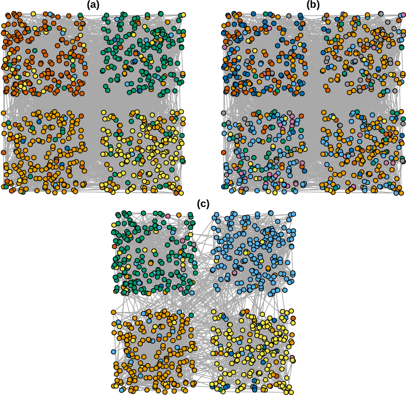
For comparison purpose, in Figure 1, we also show the results of applying CFG and Louvain algorithms on a network with 4 communities, average degree $\langle k\rangle\approx 10$ and $p_{\text{in}}=0.66$. In this case, CFG achieves modularity $Q=0.33$ and Louvain, $Q=0.31$. We apply our method in this network, setting $\alpha=0.1$. In each round, we run the dynamical system until $t=100$ with $10$ independent initial configurations. The most misaligned edge per round is removed until there is no more edges to remove. We choose the partition that yields the best modularity. The results of the iterative edge-removal process are better than those of CFG and Louvain, reaching $Q=0.38$.

Figure 2: Evolution of the modularity $Q$ over the rounds of the proposed iteration edge-removal process. The input network and learning configuration are the same presented in Figure 1. Solid and dashed horizontal lines correspond to the modularity achieved by CFG and Louvain, respectively.

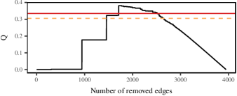
Figure 2 shows the modularity evolution over different rounds. Since communities are defined by connected components, the first edge-removal rounds just result in a single community, making the modularity score be very low. Those abrupt transitions reveal different components becoming completely disconnected from each other, i.e., they reveal those rounds in which the last edge that links two large components is removed. After achieving four major communities — and consequently the highest score —, further removal starts destroying them. Such a local optimum partition is the one that should be returned by the proposed iterative edge-removal method.

Figure 3: Evolution of the dynamics governed by Equation 1 in a network with $800$ nodes, average degree $\langle k\rangle=10$, $4$ communities, and $p_{\text{in}}=0.9$. For better visualization, even though the system has been simulated with $D=3$ dimensions and $800$ particles, only $200$ random-selected normalized velocity vectors are shown projected in two dimensions. $1000$ system iterations are run in each plot and the path of the velocity vectors are more opaque in the last iterations. Path colors match the four different communities. In plot (a), no edge was removed. In the remaining plots, 200 (b), 400 (c) and 600 (d) edges have been removed iteratively.

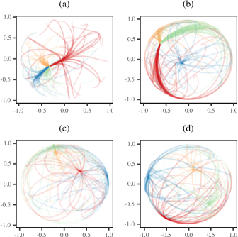
To further illustrate our method, we provide another simulation. We show (in Section III) that all the vertices in a connected component will align as time tends to infinity. As a result, one might wonder how our edge-removal strategy works in practice. To demonstrate its effectiveness, the method is applied on a simpler community detection problem: detecting the $4$ communities with the same size in a random clustered network that comprises $800$ nodes with average degree $\langle k\rangle=10$. Connections are randomly assigned such that every node has probability $p_{\text{in}}=0.9$ of connecting to another node in its community. We run our method with $3$-dimensional velocity vectors and $\alpha=0.05$. For the sake of visualization, Figure 3 depicts the evolution of the normalized velocity vectors (projected in two dimensions) in different situations. Line colors represent communities, and the transparency decreases in function of time $t$. Plot (a) depicts $1000$ iterations of our dynamical system in the original network. One can notice that all particles are aligned, but the velocity vectors of particles in different communities converge from different directions. This phenomenon is utterly important, since it enables us to distinguish the communities. It also explains the difference between our method and Kuramoto-based ones[21, 22]. In the synchronization-based techniques, each element usually is a fixed low dimensional dynamical system. In the Kuramoto oscillator model, only a single real value is associated to each node, which corresponds to the phase. Thus, nodes can only synchronize “from two different directions”. Using three or more dimensions in our method, we bring an infinitude of possible directions. In the same figure, we also show three snapshots of the edge-removal process. After running up to $t=1000$, we remove the $10$ edges with highest values of misalignment coefficient. We repeat this process until $600$ edges have been removed. The evolution of the normalized velocity vectors at $t=1,2,\dots,1000$ after removing $200$, $400$, and $600$ edges are illustrated in subplots (a), (b), and (c), respectively. After the removal of $200$ edges, we observe that one of the communities disconnects from the others, becoming a single connected component, and thus, the velocity vectors converge to a different point. With $400$ edges removed, another community detaches. And finally, after $600$ removals, each community becomes a connected component of the network, achieving our goal.

IV-B Analysis of the evolution of misalignment coefficient

Figure 4: Misalignment coefficient of the network presented in Figure 1: 4 communities, each one made of 200 vertices, $\langle k\rangle\approx 10$, and $p_{\text{in}}=0.66$. The population of coefficients is obtained from 10 independent runs. Parameter $\alpha=0.1$. Measurements are taken from a single round. Top plot: average misalignment coefficient evolution separated between intra- (dashed line) and inter-community (solid line) edges. Bottom plot: ratio between the misalignment coefficient of inter- and intra-community edges.

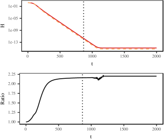
In the previous section, we claimed that the misalignment coefficients of edges connecting distinct communities become usually higher than those connecting vertices inside the same community. Let us now present, in Figure 4, how misalignment coefficients change over time.

In order to reduce the dependence on the initial condition – random assignment of velocities –, the population of misalignment coefficient values is obtained from 10 independent runs. The input network is the same for all of these runs. The network has 800 vertices and $\langle k\rangle\approx 10$, what gives a total of approximately 4000 edges.

In the top plot of Figure 4, we plot the average misalignment coefficient $H$ grouped by intra- and inter-edges. As we can see, coefficients fall down quickly. Intra-edges, however, align faster than the inter-edges. In the bottom plot, we show the ratio between intra- and inter-edges. As expected, a greater proportion of intra-edges have lower misalignment coefficient. Moreover, after many iterations, the velocity vectors become almost identical for every pair of connected vertices. At this point, the finest machine representation of real numbers is reached. The vertical dotted line indicates the iteration $t$ in which the average misalignment is lower than $10^{-12}$. Any result beyond this point might be meaningless. Consequently, we should always stop the system earlier.

IV-C Analysis of the number of removed edges

Results of removing a different number of edges per round are presented in this section. An evaluation index is used in order to objectively quantify the accuracy of the set of obtained communities. Specifically, we selected the adjusted Rand index (ARI), which is the corrected-for-chance version of the Rand index [23]. It measures the similarity between the partition obtained from some algorithm and a reference partition. ARI generates values between $-1$ and $1$. If two partitions match perfectly each other, it results in a value $1$. On the other hand, it ensures a value close to $0$ for a randomly-labelled partition or a partition that assigns all the elements into a single group, given that the reference partition has more than one group, of course. Negative values stand for some anti-correlation between the pair of partitions.

Real-world applications, however, do not provide such a reference partition, so we also employ the modularity score. Unlike ARI, the modularity score does not make any assumption on a-priori knowledge of the network, e.g., vertex labels. By placing the ARI score against the modularity score, we can check for any relationship between them, i.e., check for a relationship between an information available in a real application (modularity) and a robust measure based on reference partitions (ARI).

Figure 5: ARI (solid lines) and modularity (dashed line) scores along different rounds. The input network is exactly the same one depicted in Figure 1: 4 communities, each one made of 200 vertices, $\langle k\rangle\approx 10$, and $p_{\text{in}}=0.66$. Plots are arranged according to the amount of edges removed per round: 1, 20, and 80. For all runs, we set $\alpha=0.1$ and the system runs until $t=100$. The solid horizontal line indicates the ARI score obtained by the CFG method.

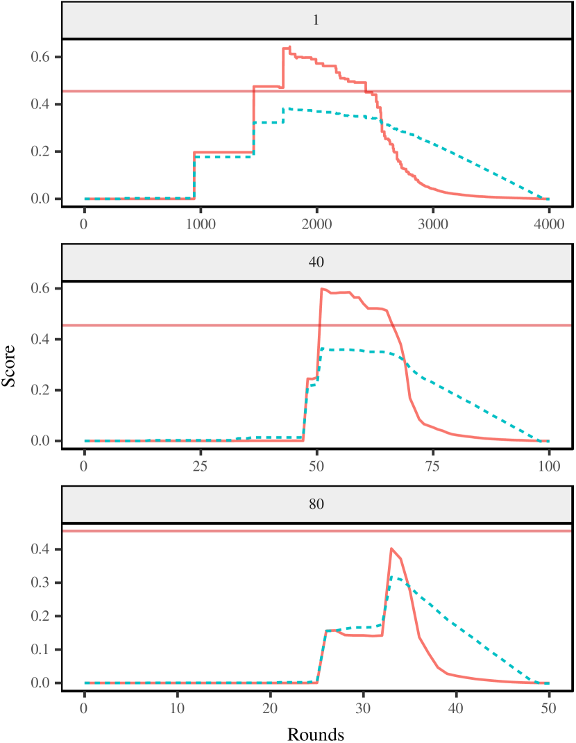
Firstly, let us consider the same network presented in Figure 1, with $p_{\text{in}}=0.66$. ARI and modularity scores along different rounds are presented in Figure 5, arranged according to the number of edges removed per round.

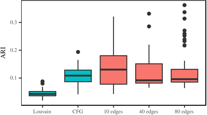
Even when 40 edges ($\approx 1\%$ of the total number of edges) are removed per round, our method achieves higher ARI score than the CFG method: $0.64$ (1 edge) and $0.60$ (40 edges) against $0.45$. Removing fewer edges per round is slightly better. Removing a larger fraction of the edges is less expensive though, for it demands fewer rounds to complete. However, we experience a significantly drop in the score if the fraction of removed edges per round is too big (around 2%.)

Moreover, a desirable relationship is noticeable here: the highest modularity matches relatively high ARI scores. This result is useful for establishing when we should stop the edge-removal process and where the optimal round is, i.e., the round after which we are likely to find a good partition: stopping the process just before the modularity starts decreasing and taking such highest-modularity’s network, using the connected components as the final set of communities. Although the results of Figure 5 come from just one network instance, the same overall pattern is still present in other instances, even using different network parameters, as we are going to see in the remaining results presented in this paper.

Figure 6: Results of removing 1, 40 and 80 edges per round on a population of 50 different networks. Each network has 4 communities, each one made of 200 vertices, $\langle k\rangle\approx 10$, and $p_{\text{in}}=0.66$. Boxes in blue are the results of applying CFG and Louvain on the network. The remaining boxes (in red) are obtained by applying the proposed technique removing different amounts of edges. The partition that yields the best modularity is chosen. 10 runs per round are performed, and parameter $\alpha=0.1$ for all simulations. We stop the system at $t=100.$

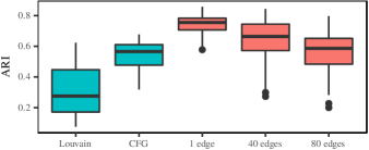
In Figure 6, we present a comparison between removing 1, 40, and 80 edges per round on a population of 50 different networks. In fact, removing a smaller fraction of the edges yields better results. In addition, the variability of results is reduced when removing less edges per round. However, the proposed edge-removal process leads to considerably better results compared to the application of CFG or Louvain on the original network.

IV-D Computational complexity

The edge-removal approach presented here is somewhat similar to the edge-betweenness-based algorithm proposed by Newman and Girvan [15]. The misalignment coefficient of an edge measures how different the incident vertices are in terms of their velocity vector. Edge betweenness, in turn, measures the relevance of an edge in terms of the number of shortest paths that include such an edge. Both concepts ultimately try to identify edges that connect distinct communities. An important drawback of the edge-betweenness approach is, however, its cubic time complexity. Precisely, for a network of $m$ edges and $n$ vertices, the time complexity is $O(m^{2}n)$, or $O(n^{3})$ for sparse networks, in which case $m\sim n$ [9, 15, 17, 12]. Therefore, it is necessary to have a discussion about the complexity of the approach proposed here.

Four variables are relevant to our time-complexity analysis: the number $n$ of vertices; the number $m$ of edges; the total amount of time-steps $t_{\text{total}}$ per run; and the number of edge-removal rounds $n_{\text{rounds}}$ required to obtain an appropriate partition of the network. The dimensionality of the velocity vectors is constant, three dimensions are employed in our experiments, so it is not relevant to this analysis. Our hypothesis is that both $t_{\text{total}}$ and $n_{\text{rounds}}$ can be invariant no matter how big the network is.

In the case of removing just a single edge per round, $n_{\text{rounds}}$ gets the order of $m$. However, the experiments presented in the previous section indicate that it is still possible to obtain satisfactory results by removing a fraction of all the edges per round, in which case $n_{\text{rounds}}$ becomes constant. For instance, removing approximately 1% of the edges per round requires around 50 rounds to achieve good results. Also, concerning the number of runs per round, if one decides to perform a set of runs per round in order to reduce the influence of the initial random configuration, the number is still relatively small and does not scale with neither $n$ nor $m$.

In order to provide evidence that supports our hypothesis – neither $t_{\text{total}}$ nor $n_{\text{rounds}}$ scales with the network size –, we present some results on bigger and denser networks. Particularly, a network that has 10 times more vertices than those studied in the previous section and a network that has twice more edges while keeping the same number of vertices.

Figure 7: Misalignment coefficient of a big and a dense network: both of them with 4 communities and $p_{\text{in}}=0.66$. The big network has 2000 vertices in each community, while the dense has 200. The average degree in the big network is $\langle k\rangle\approx 10$, while in the dense one, $\langle k\rangle\approx 20$. The population of coefficients is obtained from 10 independent runs. Parameter $\alpha=0.1$. Measurements are taken from a single round. Top plots: average misalignment coefficient evolution separated between intra- (dashed line) and inter-community (solid line) edges. Bottom plots: ratio between the misalignment coefficient of inter- and intra-community edges.

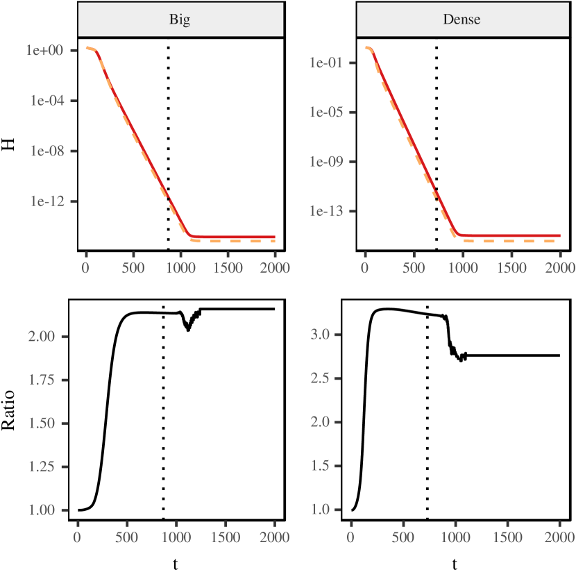
In Figure 7, we present the evolution of the coefficients in the first round. We notice that increasing the network size or the density has small effects on the amount of time-steps needed to obtain satisfactory separation. Interestingly, the bigger network requires a little more iterations while the denser one, a little less. Therefore we can estimate that, for an arbitrarily large network, $t_{\text{total}}$ remains almost the same, or at least do not scale linearly with the network size.

Figure 8: ARI (solid lines) and modularity (dashed line) scores along different rounds. Input networks are exactly the same ones depicted in Figure 7. Plots are arranged according to the amount of edges removed per round: $\approx 0.025\%$ and $1\%$. The exact number of edges removed per round is indicated between parentheses. For all runs, we set $\alpha=0.1$ and the system runs until $t=80$ for the dense network and $t=250$ for the big network. The solid horizontal line indicates the ARI score obtained by the CFG method.

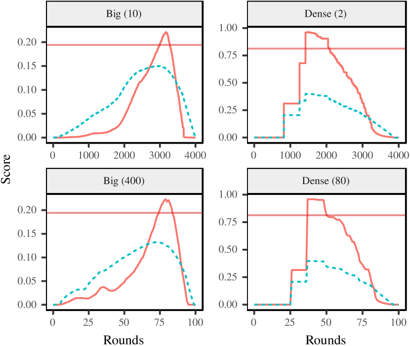
Furthermore, we analyse the scores along different rounds by running up to the iteration $t=80$ for the dense network and $t=250$ for the big network. Results are plotted in Figure 8. Both the misalignment coefficient evolution and the ARI score follow similar shapes compared with the results of smaller networks presented in the previous sections.

Since the summation in Equation 1 takes place on the set of edges, the time complexity for a single dynamical iteration $t$ is $O(m)$. Seeing that $t_{\text{total}}$ does not scale with the network size, the entire run still takes $O(m)$. In addition, at the end of each round (a single run or a small set of runs), we need to target the highest-misaligned edges, what requires sorting the set of edges and usually takes $O(m\,\text{log}\,m)$. Since $n_{\text{rounds}}$ does not scale with the network size either, then all the edge-removal process has a quasilinear time complexity: $O(m\,\text{log}\,m)$ if $m\gg n$, or just $O(n\,\text{log}\,n)$ for sparse networks.

However, it is important to emphasize that the cost $O(m\,\text{log}\,m)$ holds only from the asymptotic point of view, when networks become very large. For small- or medium-sized networks, the cost caused by $t_{\text{total}}$ and $n_{\text{rounds}}$ may become noticeable.

IV-E Experiments on unbalanced-communities networks

Figure 9: Results of removing 10, 40 and 80 edges per round on a population of 50 different networks. Each network has 4 communities, containing 800, 400, 200, and 100 vertices, $\langle k\rangle\approx 10$, and $p_{\text{in}}=0.66$. Boxes in blue are the results of applying CFG and Louvain on the network. The remaining boxes (in red) are obtained by applying the proposed technique removing different amounts of edges. The partition that yields the best modularity is chosen. 10 runs per round are performed, and parameter $\alpha=0.1$ for all simulations. We stop the system at $t=250$.

All the experiments presented so far are performed on a class of balanced networks, whose communities have the same size. In order to provide more-realistic examples, let us introduce now some results on networks whose communities have different number of vertices. These results are shown in Figure 9.

We notice now a considerable drop in the quality of the partitions. Still, compared to traditional algorithms like CFG or Louvain applied to the original network, the proposed edge-removal process performs well. The performance of the proposed method, however, varies greatly. One possible explanation is that the fixed number of iterations $t=250$ is not ideal. The study of heuristics for the system’s stop condition are left for future works.

IV-F Experiments on Lancichinetti benchmark

Since real-world networks usually have heterogeneous degree distribution, we also apply our technique on the benchmark of Lancichinetti et al.[24]. Such benchmark produces networks in which both degree and community size distributions follow power law functions with arbitrary exponents. Motivated by typical values found in natural systems, we choose exponent $2$ for the degree distribution and $1$ for the size of communities. The generated networks have a mixing parameter $\mu$ that controls the fraction of links between nodes of different communities. To assess our method, we use networks with $1000$ nodes and average degree $10$, varying the mixing parameter $\mu$ between $0.1$ and $0.6$.

We compare our method against CFG and Louvain in $30$ independent trials. The performance is measured in terms of the normalized mutual information index, which measures the similarly of the predicted partition against the expected one. Moreover, such index is suggested by the authors of the benchmark. CFG and Louvain have no parameter, while in our technique we set $\alpha=0.05$. For stopping criterion, we run the system until the maximum change in each projection $\hat{v}_{i,d}$ is less than $10^{-3}$ and remove the edge with higher misalignment coefficient. We interpret each connected component as a community. We repeat the edge-removal process until the modularity of the partitioning starts decreasing.

Figure 10: Comparison of the normalized mutual information index obtained by three community detection algorithms—our proposed method, CFG and Louvain—in the Lancichinetti et al. benchmark[24]. Results are taken from 30 independent trials for each value of the mixing parameter $\mu$. Networks contain $1000$ nodes, average degree $10$. Degree and community size distribution follow power law functions with exponents $2$ and $1$, respectively.

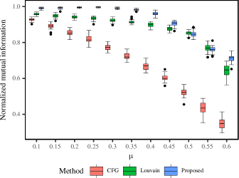
Figure 10 reveals that our method performs significantly better than CFG and Louvain. Beyond the mark $\mu=0.5$, communities are no longer defined in a strong sense since each node has more neighbors in other communities than in its own.

IV-G Experiments on real-world datasets

We apply our algorithm to four well-known real-world networks: Zachary’s karate club [25], the bottlenose dolphins social network [26], the American College Football [27], and the Krebs’ books on US politics.

TABLE I: Modularity score of community detection methods in 4 classic real-world datasets. Optimal modularity is shown for comparison.

Method	Dolphin	Football	Karate	Political Books
Proposed	0.529	0.605	0.419	0.527
Amiri [28]	0.515	0.597	0.417	0.518
Honghao [29]	0.529	0.605	0.420	0.527
Song [30]	-	0.531	0.362	0.463
Optimal	0.529	0.605	0.420	-

Table I presents the best modularity scores obtained by our method. We set $\alpha=0.1$, $30$ independent runs, and vary the fraction of removed edges in $1\%$, $2\%$, …, $10\%$. Also, we vary the number of iterations $t\in[30,70]$. We compare our results against three other bio-inspired optimization methods. (Missing results have not been measured by the authors of the original paper.) Also, the optimal value of modularity is calculated using an exhaustive search in all possible partitions. Modularity optimization is an NP-complete problem, and known algorithms have exponential time complexity [15]. (We were not able to find out the optimal partition of the political books network.)

We observe that our method reached either optimal or nearly-optimal modularity scores. Although the ant-colony-based technique [29] had similar performance, our algorithm has lower computational cost because it explores the solution space in a greedy manner.

V Conclusions

Throughout an extensive set of experiments presented in this paper, we see that the proposed flocking-like dynamical system and the iterative edge-removal process performs well in many scenarios. The decentralized, self-organizing dynamical model is robust, thus applicable on a wide variety of networks.

The concept of misalignment coefficient defined here is, in some sense, similar to the concept of edge betweenness. High-misaligned edges are supposed to link distinct communities. However, the cost $O(n^{3})$ (on sparse networks) of the method proposed by Newman and Girvan [15] can be prohibitive for its application in large networks. On the other hand, we claim that our edge-removal process is asymptotically quasilinear: $O(n\,\text{log}\,n)$, which is quite attractive for large-network community detection.

In further works, we will study heuristics to find out good values of the number of iterations and removed edges per round.

References

- [1] F. A. N. Verri, P. R. Urio, and L. Zhao, “Network unfolding map by vertex-edge dynamics modeling,” IEEE Transactions on Neural Networks and Learning Systems, vol. PP, no. 99, 2016.
- [2] C. Pizzuti, “Evolutionary Computation for Community Detection in Networks: a Review,” IEEE Transactions on Evolutionary Computation, vol. X, no. X, pp. 1–1, 2017.
- [3] Q. Cai, M. Gong, S. Ruan, Q. Miao, and H. Du, “Network structural balance based on evolutionary multiobjective optimization: A two-step approach,” IEEE Transactions on Evolutionary Computation, vol. 19, no. 6, pp. 903–916, 2015.
- [4] P. Lv, J. Zhang, and H. Zhang, “A social network graphics segmentation algorithm based on community-detection,” in 2016 2nd IEEE International Conference on Computer and Communications (ICCC), 2016, pp. 619–623.
- [5] Z.-K. Gao, Y.-X. Yang, P.-C. Fang, N.-D. Jin, C.-Y. Xia, and L.-D. Hu, “Multi-frequency complex network from time series for uncovering oil-water flow structure,” Scientific Reports, vol. 5, 2015.
- [6] C. Thiemann, F. Theis, D. Grady, R. Brune, and D. Brockmann, “The structure of borders in a small world,” PLoS ONE, vol. 5, no. 11, 2010.
- [7] C. Zhong, S. M. Arisona, X. Huang, M. Batty, and G. Schmitt, “Detecting the dynamics of urban structure through spatial network analysis,” International Journal of Geographical Information Science, vol. 28, no. 11, pp. 2178–2199, 2014.
- [8] E. M. Heemskerk and F. W. Takes, “The corporate elite community structure of global capitalism,” New Political Economy, vol. 21, no. 1, pp. 90–118, 2016.
- [9] A. Clauset, M. E. J. Newman, and C. Moore, “Finding community structure in very large networks,” Physical Review E, vol. 70, no. 6, 2004.
- [10] M. G. Quiles, E. E. N. Macau, and N. Rubido, “Dynamical detection of network communities,” Scientific Reports, vol. 6, 2016.
- [11] T. C. Silva and L. Zhao, Machine learning in complex networks. Springer International Publishing, 2016.
- [12] S. Fortunato, “Community detection in graphs,” Physics Reports, vol. 486, no. 3–5, pp. 75–174, 2010.
- [13] M. Mitrović and B. Tadić, “Spectral and dynamical properties in classes of sparse networks with mesoscopic inhomogeneities,” Physical Review E, vol. 80, no. 2, 2009.
- [14] E. Agliari and F. Tavani, “The exact Laplacian spectrum for the Dyson hierarchical network,” Scientific Reports, vol. 7, p. 39962, 2017.
- [15] M. E. J. Newman and M. Girvan, “Finding and evaluating community structure in networks,” Physical Review E, vol. 69, no. 2, 2004.
- [16] A. Lancichinetti and S. Fortunato, “Limits of modularity maximization in community detection,” Physical Review E, vol. 84, no. 6, 2011.
- [17] ——, “Community detection algorithms: a comparative analysis,” Physical Review E, vol. 80, no. 5, 2009.
- [18] V. D. Blondel, J.-L. Guillaume, R. Lambiotte, and E. Lefebvre, “Fast unfolding of communities in large networks,” Journal of Statistical Mechanics: Theory and Experiment, vol. 2008, no. 10, 2008.
- [19] K. H. Nagai, Y. Sumino, R. Montagne, I. S. Aranson, and H. Chaté, “Collective motion of self-propelled particles with memory,” Physical Review Letters, vol. 114, no. 16, 2015.
- [20] T. Vicsek and A. Zafeiris, “Collective motion,” Physics Reports, vol. 517, pp. 71–140, 2012.
- [21] E. Oh, K. Rho, H. Hong, and B. Kahng, “Modular synchronization in complex networks,” Physical Review E, vol. 72, no. 4, p. 047101, 2005.
- [22] A. Arenas, A. Díaz-Guilera, J. Kurths, Y. Moreno, and C. Zhou, “Synchronization in complex networks,” Physics Reports, vol. 469, no. 3, pp. 93–153, 2008.
- [23] L. Hubert and P. Arabie, “Comparing partitions,” Journal of Classification, vol. 2, no. 1, pp. 193–218, 1985.
- [24] A. Lancichinetti, S. Fortunato, and F. Radicchi, “Benchmark graphs for testing community detection algorithms,” Physical Review E, vol. 78, no. 4, p. 046110, 2008.
- [25] W. Zachary, “An information flow model for conflict and fission in small groups,” Journal of Anthropological Research, vol. 33, no. 4, pp. 452–473, 1977.
- [26] O. B. P. H. E. S. D. Lusseau, K. Schneider and S. Dawson, “The bottlenose dolphin community of doubtful sound features a large proportion of long-lasting associations,” Behavioral Ecology and Sociobiology, vol. 54, no. 4, pp. 396–405, 2003.
- [27] M. Girvan and M. E. J. Newman, “Community structure in social and biological networks,” Proceedings of the National Academy of Sciences, vol. 99, no. 12, pp. 7821–7826, 2002.
- [28] B. Amiri, L. Hossain, J. W. Crawford, and R. T. Wigand, “Community detection in complex networks: Multi–objective enhanced firefly algorithm,” Knowledge-Based Systems, vol. 46, no. Supplement C, pp. 1 – 11, 2013.
- [29] C. Honghao, F. Zuren, and R. Zhigang, “Community detection using ant colony optimization,” in 2013 IEEE Congress on Evolutionary Computation, 2013, pp. 3072–3078.
- [30] A. Song, M. Li, X. Ding, W. Cao, and K. Pu, International Journal of Computer Science, no. 1, pp. 37–44.