Technical report

Probabilistic modelling and reconstruction of strain

Carl Jidling, Johannes Hendriks, Niklas Wahlström, Alexander Gregg, Thomas B. Schön, Christopher Wensrich and Adrian Wills

  • \bullet

    Please cite this version:
    Carl Jidling, Johannes Hendriks, Niklas Wahlström, Alexander Gregg, Thomas B. Schön, Christopher Wensrich and Adrian Wills. Probabilistic modelling and reconstruction of strain. Nuclear instruments and methods in physics research section B, 436:141-155, 2018.

This paper deals with modelling and reconstruction of strain fields, relying upon data generated from neutron Bragg-edge measurements. We propose a probabilistic approach in which the strain field is modelled as a Gaussian process, assigned a covariance structure customised by incorporation of the so-called equilibrium constraints. The computational complexity is significantly reduced by utilising an approximation scheme well suited for the problem. We illustrate the method on simulations and real data. The results indicate a high potential and can hopefully inspire the concept of probabilistic modelling to be used within other tomographic applications as well.

Abstract

This paper deals with modelling and reconstruction of strain fields, relying upon data generated from neutron Bragg-edge measurements. We propose a probabilistic approach in which the strain field is modelled as a Gaussian process, assigned a covariance structure customised by incorporation of the so-called equilibrium constraints. The computational complexity is significantly reduced by utilising an approximation scheme well suited for the problem. We illustrate the method on simulations and real data. The results indicate a high potential and can hopefully inspire the concept of probabilistic modelling to be used within other tomographic applications as well.

1 Introduction

The goal of tomographic reconstruction is to build a map of an unknown quantity within an object using information gained from irradiation experiments. A well known example of this is X-ray imaging, where the unknown quantity might be, for instance, the bone density inside a human body.

Each measurement provides information about the amount of intensity that the ray has lost when passing through the material. Of course, a single measurement does not uniquely define the interior. However, processing a large number of measurements taken from many different angles allows for an accurate reconstruction of the internal structure.

While techniques such as X-ray imaging and MRI are concerned with scalar fields, we are in this work considering the reconstruction of the strain field – a second order tensor – within a deformed material. This is a significantly harder problem as it is a multidimensional quantity at each point. For simplicity, we are restricting the analysis to a planar problem, but the extension to three dimensions follows the same procedure.

The development of accurate strain measuring techniques is motivated by applications within several fields. One field with perhaps especially exciting application potential is additive manufacturing, which involves printing of three-dimensional metal structures. For instance, this is of interest for developers of fuel nozzles (Tremsin et al.,, 2016) and turbine blades (Watkins et al.,, 2013) within the aerospace industry.

Several techniques enabling high-precision measurement of residual strain have been proposed in previous work. These are characterised as destructive, semi-destructive or non-destructive, where examples from each category includes slitting (Prime,, 2001), ring-coring (Standard, ASTM and others,, 2002) and diffraction (Fitzpatrick and Lodini,, 2003; Noyan and Cohen,, 2013), respectively.

Bragg-edge analysis (Santisteban et al., 2002a, ; Santisteban et al., 2002b, ) is an alternative transmission-based approach aiming at reconstructing the entire three-dimensional strain-field. This is an important difference to the established techniques outlined above, including the diffraction-based strain tomography such as synchrotron X-ray measurements (Korsunsky et al.,, 2011, 2008). The term Bragg-edge refers to rapid changes in the relative transmission rate, which are determined from Bragg’s law and hence directly related to the wavelength (Santisteban et al., 2002b, ).

Methods relying on the Bragg-edge idea have seen a significant progress during recent years, and provides an essential foundation for generation of high-resolution strain-images within polycrystalline materials (Santisteban et al., 2002a, ; Tremsin et al.,, 2012, 2011; Woracek et al.,, 2018).

A practical method based on the Brag-edge technique has been proposed by Wensrich et al., 2016b . This relies upon the assumption that the strain field is compatible (see Section D), which allows the measurement equation to be expressed in terms of the boundary displacements. The reconstruction is obtained by solving a least squares problem and providing the result as a boundary condition to a finite element solver. An extension of this method is given by Wensrich et al., 2016a with application to a real-world problem presented in (Hendriks et al.,, 2017).

The solution technique presented in this work relies upon the concept of probabilistic modelling (Ghahramani,, 2015). Probabilistic modelling refers to methods that are employing probability theory to encode uncertainties present in the problem and where the solution is obtained through statistical inference. The idea is based on the assumption that uncertainties are always present, mainly due to a limited amount of data and the presence of measurement noise. A natural way of encoding these uncertainties in the model is therefore to assign a probabilistic measure to the unknown quantities themselves.

The contribution of this paper is a new way of modelling and reconstructing strain fields from data generated by neutron Bragg-edge measurements. We are using a tailored Gaussian process (GP)(Rasmussen and Williams,, 2006) to model the strain field, and by utilising the fact that GPs are closed under linear transformations, the reconstruction of the strain field is obtained through GP regression. The model is customised by designing the associated covariance function with respect to the so-called equilibrium constraints, which guarantees a physical solution.

2 Problem formulation

Given a set of measurements generated from a neutron Bragg-edge experiment, the problem faced in this work is to reconstruct the strain at various positions within a sample. The sample is an object, in which we want to reconstruct strain. The sample is considered to be two-dimensional. The strain in such a sample can be represented using a symmetric 2×2222\times 2-matrix ϵbold-italic-ϵ\mathbf{\boldsymbol{\mathrm{\epsilon}}} called the strain tensor. Any point in the sample has an assigned strain tensor. This assignment is described by the strain field ϵ(𝐱)bold-italic-ϵ𝐱\mathbf{\boldsymbol{\mathrm{\epsilon}}}(\mathbf{\boldsymbol{\mathrm{x}}}), which is a function mapping any point in space 𝐱=[x,y]𝖳2𝐱superscript𝑥𝑦𝖳superscript2\mathbf{\boldsymbol{\mathrm{x}}}=[x,\,\,y]^{\mathsf{T}}\in\mathbb{R}^{2} to a strain tensor ϵbold-italic-ϵ\mathbf{\boldsymbol{\mathrm{\epsilon}}}. The strain field can be construed as

ϵ(𝐱)=[ϵxx(𝐱)ϵxy(𝐱)ϵyx(𝐱)ϵyy(𝐱)]2×2,bold-italic-ϵ𝐱matrixsubscriptitalic-ϵ𝑥𝑥𝐱subscriptitalic-ϵ𝑥𝑦𝐱subscriptitalic-ϵ𝑦𝑥𝐱subscriptitalic-ϵ𝑦𝑦𝐱superscript22\mathbf{\boldsymbol{\mathrm{\epsilon}}}(\mathbf{\boldsymbol{\mathrm{x}}})=\begin{bmatrix}\epsilon_{xx}(\mathbf{\boldsymbol{\mathrm{x}}})&\epsilon_{xy}(\mathbf{\boldsymbol{\mathrm{x}}})\\ \epsilon_{yx}(\mathbf{\boldsymbol{\mathrm{x}}})&\epsilon_{yy}(\mathbf{\boldsymbol{\mathrm{x}}})\end{bmatrix}\in\mathbb{R}^{2\times 2}, (1)

where ϵxy(𝐱)=ϵyx(𝐱)subscriptitalic-ϵ𝑥𝑦𝐱subscriptitalic-ϵ𝑦𝑥𝐱\epsilon_{xy}(\mathbf{\boldsymbol{\mathrm{x}}})=\epsilon_{yx}(\mathbf{\boldsymbol{\mathrm{x}}}) since strain tensors are symmetric.

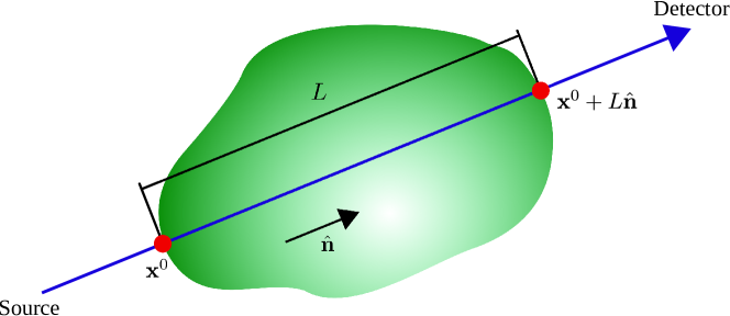
The experiments rely upon high resolution time-of-flight neutron detectors. Neutron beams are generated at a source, transmitted through the sample, and recorded at a detector located at the opposite side of the sample. Considering a single measurement, assume that the neutrons enters the sample at a point 𝐱0superscript𝐱0\mathbf{\boldsymbol{\mathrm{x}}}^{0}, propagates along the direction defined by the unit vector 𝐧^^𝐧\hat{\mathbf{n}} and exits at 𝐱0+L𝐧^superscript𝐱0𝐿^𝐧\mathbf{\boldsymbol{\mathrm{x}}}^{0}+L\hat{\mathbf{n}}, where L𝐿L is the illuminated distance in the sample. This is illustrated in Fig. 1. An ideal measurement obtained from the neutron Bragg-edge method can be expressed in terms of the Longitudinal Ray Transform (LRT)

I(𝜼)=1L0L𝐧^𝖳ϵ(𝐱0+s𝐧^)𝐧^𝑑s,I𝜼1𝐿superscriptsubscript0𝐿superscript^𝐧𝖳bold-italic-ϵsuperscript𝐱0𝑠^𝐧^𝐧differential-d𝑠\mathrm{I}(\mathbf{\boldsymbol{\mathrm{\eta}}})=\frac{1}{L}\int_{0}^{L}\hat{\mathbf{n}}^{\mathsf{T}}\mathbf{\boldsymbol{\mathrm{\epsilon}}}(\mathbf{\boldsymbol{\mathrm{x}}}^{0}+s\hat{\mathbf{n}})\hat{\mathbf{n}}ds, (2)

where 𝜼={𝐱0,L,𝐧^}𝜼superscript𝐱0𝐿^𝐧\mathbf{\boldsymbol{\mathrm{\eta}}}=\{\mathbf{\boldsymbol{\mathrm{x}}}^{0},L,\hat{\mathbf{n}}\} specifies the argument of the LRT and where s𝑠s is a coordinate used to specify the position on the line between the entry and exit points. We can interpret (2) as the average strain along the propagated path, so the LRT plays an important role in defining an adequate measurement model within this framework (Lionheart and Withers,, 2015). See A for some more details on the Bragg-edge experiment.
Refer to caption
Figure 1: Experimental setup. The neutrons are transmitted from a source through the sample along the line starting at 𝐱0superscript𝐱0\mathbf{\boldsymbol{\mathrm{x}}}^{0} and ending at 𝐱0+𝐧^Lsuperscript𝐱0^𝐧𝐿\mathbf{\boldsymbol{\mathrm{x}}}^{0}+\hat{\mathbf{\mathbf{\boldsymbol{\mathrm{n}}}}}L and finally measured by a detector.

In a real-world application, we will have access to a data set 𝒟={(𝜼i,yi)}i=1N𝒟superscriptsubscriptsubscript𝜼𝑖subscript𝑦𝑖𝑖1𝑁\mathcal{D}=\{(\mathbf{\boldsymbol{\mathrm{\eta}}}_{i},y_{i})\}_{i=1}^{N} with

yi=I(𝜼i)+εi,subscript𝑦𝑖Isubscript𝜼𝑖subscript𝜀𝑖y_{i}=\mathrm{I}(\mathbf{\boldsymbol{\mathrm{\eta}}}_{i})+\varepsilon_{i}, (3)

where εisubscript𝜀𝑖\varepsilon_{i} denotes the measurement noise. Hence, the problem to be solved is this: Given the measurements {yi}i=1Nsuperscriptsubscriptsubscript𝑦𝑖𝑖1𝑁\{y_{i}\}_{i=1}^{N} in (3) and the relation (2), reconstruct the strain tensor (1) in any arbitrary test point 𝐱subscript𝐱\mathbf{\boldsymbol{\mathrm{x}}}_{*} along with an uncertainty measure of the accuracy for this reconstruction.

3 Strain field reconstruction using Gaussian processes

In this work, the problem is solved by making use of the framework known as probabilistic modelling, with the somehow abstract idea of assigning a probability distribution to the strain field. This does not mean that we should think of the strain field as a random object, but the distribution provides a way for us to encode the uncertainty of the reconstruction. The presence of the uncertainty is mainly due to the fact that we have a finite number of measurements and that each of these measurements by construction are contaminated with noise.

More specifically, to reconstruct the strain field based on LRT measurements (2), we need a probabilistic model describing (i) the strain field, and (ii) the relation between the strain field and the measurements. The model should be able to reason about the uncertainties present in the measurements and take known physical constraints into consideration. In this work we choose to model the strain field with a Gaussian process.

3.1 Gaussian processes

A GP is a stochastic process suitable for modelling spatially correlated measurements. GPs can be seen as a distribution over functions

𝐟(𝐱)𝐟𝐱\displaystyle\mathbf{\boldsymbol{\mathrm{f}}}(\mathbf{\boldsymbol{\mathrm{x}}}) 𝒢𝒫(𝐦(𝐱),𝐊(𝐱,𝐱)),similar-toabsent𝒢𝒫𝐦𝐱𝐊𝐱superscript𝐱\displaystyle\sim\mathcal{GP}\big{(}\mathbf{\boldsymbol{\mathrm{m}}}(\mathbf{\boldsymbol{\mathrm{x}}}),\mathbf{\boldsymbol{\mathrm{K}}}(\mathbf{\boldsymbol{\mathrm{x}}},\mathbf{\boldsymbol{\mathrm{x}}}^{\prime})\big{)}, (4)

where the process is uniquely defined with its mean function 𝐦(𝐱)=𝔼[𝐟(𝐱)]𝐦𝐱𝔼delimited-[]𝐟𝐱\mathbf{\boldsymbol{\mathrm{m}}}(\mathbf{\boldsymbol{\mathrm{x}}})=\mathbb{E}[\mathbf{\boldsymbol{\mathrm{f}}}(\mathbf{\boldsymbol{\mathrm{x}}})] and covariance function 𝐊(𝐱,𝐱)=𝔼[(𝐟(𝐱)𝐦(𝐱))(𝐟(𝐱)𝐦(𝐱))𝖳]𝐊𝐱superscript𝐱𝔼delimited-[]𝐟𝐱𝐦𝐱superscript𝐟superscript𝐱𝐦superscript𝐱𝖳\mathbf{\boldsymbol{\mathrm{K}}}(\mathbf{\boldsymbol{\mathrm{x}}},\mathbf{\boldsymbol{\mathrm{x}}}^{\prime})=\mathbb{E}\big{[}(\mathbf{\boldsymbol{\mathrm{f}}}(\mathbf{\boldsymbol{\mathrm{x}}})-\mathbf{\boldsymbol{\mathrm{m}}}(\mathbf{\boldsymbol{\mathrm{x}}}))(\mathbf{\boldsymbol{\mathrm{f}}}(\mathbf{\boldsymbol{\mathrm{x}}}^{\prime})-\mathbf{\boldsymbol{\mathrm{m}}}(\mathbf{\boldsymbol{\mathrm{x}}}^{\prime}))^{\mathsf{T}}\big{]}. The GP is a generalisation of the multivariate Gaussian probability distribution in the sense that the function values evaluated for a finite number of inputs 𝐱1,,𝐱Nsubscript𝐱1subscript𝐱𝑁\mathbf{\boldsymbol{\mathrm{x}}}_{1},\dots,\mathbf{\boldsymbol{\mathrm{x}}}_{N} are Gaussian distributed

[𝐟(𝐱1)𝐟(𝐱N)]matrix𝐟subscript𝐱1𝐟subscript𝐱𝑁\displaystyle\begin{bmatrix}\mathbf{\boldsymbol{\mathrm{f}}}(\mathbf{\boldsymbol{\mathrm{x}}}_{1})\\ \vdots\\ \mathbf{\boldsymbol{\mathrm{f}}}(\mathbf{\boldsymbol{\mathrm{x}}}_{N})\end{bmatrix} 𝒩(𝝁,𝐊),where𝝁=[𝐦(𝐱1)𝐦(𝐱N)],formulae-sequencesimilar-toabsent𝒩𝝁𝐊where𝝁matrix𝐦subscript𝐱1𝐦subscript𝐱𝑁\displaystyle\sim{\mathcal{N}}(\mathbf{\boldsymbol{\mathrm{\mu}}},\mathbf{\boldsymbol{\mathrm{K}}}),\quad\text{where}\quad\mathbf{\boldsymbol{\mathrm{\mu}}}=\begin{bmatrix}\mathbf{\boldsymbol{\mathrm{m}}}(\mathbf{\boldsymbol{\mathrm{x}}}_{1})\\ \vdots\\ \mathbf{\boldsymbol{\mathrm{m}}}(\mathbf{\boldsymbol{\mathrm{x}}}_{N})\end{bmatrix}, (5a)
and
𝐊𝐊\displaystyle\mathbf{\boldsymbol{\mathrm{K}}} =[𝐊(𝐱1,𝐱1)𝐊(𝐱1,𝐱N)𝐊(𝐱N,𝐱1)𝐊(𝐱N,𝐱N)].absentmatrix𝐊subscript𝐱1subscript𝐱1𝐊subscript𝐱1subscript𝐱𝑁missing-subexpression𝐊subscript𝐱𝑁subscript𝐱1𝐊subscript𝐱𝑁subscript𝐱𝑁\displaystyle=\begin{bmatrix}\mathbf{\boldsymbol{\mathrm{K}}}(\mathbf{\boldsymbol{\mathrm{x}}}_{1},\mathbf{\boldsymbol{\mathrm{x}}}_{1})&\cdots&\mathbf{\boldsymbol{\mathrm{K}}}(\mathbf{\boldsymbol{\mathrm{x}}}_{1},\mathbf{\boldsymbol{\mathrm{x}}}_{N})\\ \vdots&&\vdots\\ \mathbf{\boldsymbol{\mathrm{K}}}(\mathbf{\boldsymbol{\mathrm{x}}}_{N},\mathbf{\boldsymbol{\mathrm{x}}}_{1})&\cdots&\mathbf{\boldsymbol{\mathrm{K}}}(\mathbf{\boldsymbol{\mathrm{x}}}_{N},\mathbf{\boldsymbol{\mathrm{x}}}_{N})\end{bmatrix}. (5b)

In this work we will only consider zero-mean GPs, i.e., where 𝐦(𝐱)=𝟎𝐦𝐱0\mathbf{\boldsymbol{\mathrm{m}}}(\mathbf{\boldsymbol{\mathrm{x}}})=\mathbf{\boldsymbol{\mathrm{0}}}. This is the natural choice in absence of more specific prior knowledge. It shall not be interpreted as if we believe that 𝐟(𝐱)=𝟎𝐟𝐱0\mathbf{\boldsymbol{\mathrm{f}}}(\mathbf{\boldsymbol{\mathrm{x}}})=\mathbf{\boldsymbol{\mathrm{0}}}, it simply represents the fact that we do not have any better initial guess.

Since ϵ(𝐱)bold-italic-ϵ𝐱\mathbf{\boldsymbol{\mathrm{\epsilon}}}(\mathbf{\boldsymbol{\mathrm{x}}}) is a symmetric 2×2222\times 2 tensor, it consists of three unknown components, ϵxx(𝐱)subscriptitalic-ϵ𝑥𝑥𝐱\epsilon_{xx}(\mathbf{\boldsymbol{\mathrm{x}}}), ϵxy(𝐱)subscriptitalic-ϵ𝑥𝑦𝐱\epsilon_{xy}(\mathbf{\boldsymbol{\mathrm{x}}}) and ϵyy(𝐱)subscriptitalic-ϵ𝑦𝑦𝐱\epsilon_{yy}(\mathbf{\boldsymbol{\mathrm{x}}}). We therefore choose to model the strain tensor with a function 𝐟(𝐱):23:𝐟𝐱maps-tosuperscript2superscript3\mathbf{\boldsymbol{\mathrm{f}}}(\mathbf{\boldsymbol{\mathrm{x}}}):\mathbb{R}^{2}\mapsto\mathbb{R}^{3}, here called the strain function, where

𝐟(𝐱)=[fxx(𝐱)fxy(𝐱)fyy(𝐱)]=[ϵxx(𝐱)ϵxy(𝐱)ϵyy(𝐱)]and𝐱=[xy].formulae-sequence𝐟𝐱matrixsubscript𝑓𝑥𝑥𝐱subscript𝑓𝑥𝑦𝐱subscript𝑓𝑦𝑦𝐱matrixsubscriptitalic-ϵ𝑥𝑥𝐱subscriptitalic-ϵ𝑥𝑦𝐱subscriptitalic-ϵ𝑦𝑦𝐱and𝐱matrix𝑥𝑦\displaystyle\mathbf{\boldsymbol{\mathrm{f}}}(\mathbf{\boldsymbol{\mathrm{x}}})=\begin{bmatrix}f_{xx}(\mathbf{\boldsymbol{\mathrm{x}}})\\ f_{xy}(\mathbf{\boldsymbol{\mathrm{x}}})\\ f_{yy}(\mathbf{\boldsymbol{\mathrm{x}}})\\ \end{bmatrix}=\begin{bmatrix}\epsilon_{xx}(\mathbf{\boldsymbol{\mathrm{x}}})\\ \epsilon_{xy}(\mathbf{\boldsymbol{\mathrm{x}}})\\ \epsilon_{yy}(\mathbf{\boldsymbol{\mathrm{x}}})\\ \end{bmatrix}\qquad\text{and}\qquad\mathbf{\boldsymbol{\mathrm{x}}}=\begin{bmatrix}x\\ y\end{bmatrix}. (6)

We then put a GP prior on 𝐟(𝐱)𝐟𝐱\mathbf{\boldsymbol{\mathrm{f}}}(\mathbf{\boldsymbol{\mathrm{x}}}) according to (4). The model now consist of two parts:

  1. 1.

    The GP prior (4) of the strain field, i.e., our choice of 𝐊(𝐱,𝐱)𝐊𝐱superscript𝐱\mathbf{\boldsymbol{\mathrm{K}}}(\mathbf{\boldsymbol{\mathrm{x}}},\mathbf{\boldsymbol{\mathrm{x}}}^{\prime}). This GP prior is described in Section 3.2.

  2. 2.

    The joint distribution between the measurements 𝐲=[y1,y2,,yN]𝖳𝐲superscriptsubscript𝑦1subscript𝑦2subscript𝑦𝑁𝖳\mathbf{\boldsymbol{\mathrm{y}}}=[y_{1},\,y_{2},\,\dots,y_{N}]^{\mathsf{T}} and the strain function 𝐟=𝐟(𝐱)subscript𝐟𝐟subscript𝐱\mathbf{\boldsymbol{\mathrm{f}}}_{*}=\mathbf{\boldsymbol{\mathrm{f}}}(\mathbf{\boldsymbol{\mathrm{x}}}_{*}) at a point 𝐱subscript𝐱\mathbf{\boldsymbol{\mathrm{x}}}_{*} where we want to make a reconstruction. This distribution allows us to infer the measurements and it is described in Section 3.3 and Section 3.4.

3.2 The covariance function

The strain function cannot be any arbitrary function mapping 2superscript2\mathbb{R}^{2} to 3superscript3\mathbb{R}^{3}. It needs to obey some physical laws. Therefore, we want to model the covariance function 𝐊(𝐱,𝐱)𝐊𝐱superscript𝐱\mathbf{\boldsymbol{\mathrm{K}}}(\mathbf{\boldsymbol{\mathrm{x}}},\mathbf{\boldsymbol{\mathrm{x}}}^{\prime}) such that any sample we draw from the GP prior (4) is a valid strain function. More specifically we need to fulfil the equilibrium constraints, which for isotropic linearly elastic (i.e. in the absence of strong grain texture) solid materials under the assumption of plane stress, read as

fxx(𝐱)x+(1ν)fxy(𝐱)y+νfyy(𝐱)x=0,subscript𝑓𝑥𝑥𝐱𝑥1𝜈subscript𝑓𝑥𝑦𝐱𝑦𝜈subscript𝑓𝑦𝑦𝐱𝑥0\displaystyle\frac{\partial f_{xx}(\mathbf{\boldsymbol{\mathrm{x}}})}{\partial x}+(1-\nu)\frac{\partial f_{xy}(\mathbf{\boldsymbol{\mathrm{x}}})}{\partial y}+\nu\frac{\partial f_{yy}(\mathbf{\boldsymbol{\mathrm{x}}})}{\partial x}=0, (7a)
νfxx(𝐱)y+(1ν)fxy(𝐱)x+fyy(𝐱)y=0,𝜈subscript𝑓𝑥𝑥𝐱𝑦1𝜈subscript𝑓𝑥𝑦𝐱𝑥subscript𝑓𝑦𝑦𝐱𝑦0\displaystyle\nu\frac{\partial f_{xx}(\mathbf{\boldsymbol{\mathrm{x}}})}{\partial y}+(1-\nu)\frac{\partial f_{xy}(\mathbf{\boldsymbol{\mathrm{x}}})}{\partial x}+\frac{\partial f_{yy}(\mathbf{\boldsymbol{\mathrm{x}}})}{\partial y}=0, (7b)

where ν𝜈\nu denotes Poisson’s ratio. For 𝐟(𝐱)𝐟𝐱\mathbf{\boldsymbol{\mathrm{f}}}(\mathbf{\boldsymbol{\mathrm{x}}}) to fulfill these constraints we can describe it as a transformation of another scalar function φ(𝐱):3:𝜑𝐱maps-tosuperscript3\varphi(\mathbf{\boldsymbol{\mathrm{x}}}):\,\mathbb{R}^{3}\mapsto\mathbb{R} via the transfomation according to

𝐟(𝐱)=[2y2ν2x2(1+ν)2xy2x2ν2y2]φ(𝐱)=𝐱φ.𝐟𝐱matrixsuperscript2superscript𝑦2𝜈superscript2superscript𝑥21𝜈superscript2𝑥𝑦superscript2superscript𝑥2𝜈superscript2superscript𝑦2𝜑𝐱subscript𝐱𝜑\mathbf{\boldsymbol{\mathrm{f}}}(\mathbf{\boldsymbol{\mathrm{x}}})=\begin{bmatrix}\frac{\partial^{2}}{\partial y^{2}}-\nu\frac{\partial^{2}}{\partial x^{2}}\\[2.84526pt] (1+\nu)\frac{\partial^{2}}{\partial x\partial y}\\[2.84526pt] \frac{\partial^{2}}{\partial x^{2}}-\nu\frac{\partial^{2}}{\partial y^{2}}\end{bmatrix}\varphi(\mathbf{\boldsymbol{\mathrm{x}}})=\mathcal{L}_{\mathbf{\boldsymbol{\mathrm{x}}}}\varphi. (8)

Here, 𝐱subscript𝐱\mathcal{L}_{\mathbf{\boldsymbol{\mathrm{x}}}} is an operator mapping scalar potential functions φ(𝐱)𝜑𝐱\varphi(\mathbf{\boldsymbol{\mathrm{x}}}) to vector-valued strain functions 𝐟(𝐱)𝐟𝐱\mathbf{\boldsymbol{\mathrm{f}}}(\mathbf{\boldsymbol{\mathrm{x}}}), i.e., in this case we have 𝐱:(2)(23):subscript𝐱maps-tomaps-tosuperscript2maps-tosuperscript2superscript3\mathcal{L}_{\mathbf{\boldsymbol{\mathrm{x}}}}:(\mathbb{R}^{2}\mapsto\mathbb{R})\mapsto(\mathbb{R}^{2}\mapsto\mathbb{R}^{3}). One can easily verify that the strain function in (8) fulfils the constraints in (7). This transformation is derived from the underlying physics where φ(𝐱)𝜑𝐱\varphi(\mathbf{\boldsymbol{\mathrm{x}}}) is a known physical potential called the Airy stress function, for details, see C. We can also derive the transformation 𝐟(𝐱)=𝐱φ𝐟𝐱subscript𝐱𝜑\mathbf{\boldsymbol{\mathrm{f}}}(\mathbf{\boldsymbol{\mathrm{x}}})=\mathcal{L}_{\mathbf{\boldsymbol{\mathrm{x}}}}\varphi from any set of linear constraints, for example those presented in (7), following the procedure described by Jidling et al., (2017).

Instead of designing a covariance function for the strain function 𝐟(𝐱)𝐟𝐱\mathbf{\boldsymbol{\mathrm{f}}}(\mathbf{\boldsymbol{\mathrm{x}}}), we design a GP prior for the scalar potential function φ(𝐱)𝜑𝐱\varphi(\mathbf{\boldsymbol{\mathrm{x}}})

φ(𝐱)𝜑𝐱\displaystyle\varphi(\mathbf{\boldsymbol{\mathrm{x}}}) 𝒢𝒫(0,kφ(𝐱,𝐱)).similar-toabsent𝒢𝒫0subscript𝑘𝜑𝐱superscript𝐱\displaystyle\sim\mathcal{GP}\big{(}0,k_{\varphi}(\mathbf{\boldsymbol{\mathrm{x}}},\mathbf{\boldsymbol{\mathrm{x}}}^{\prime})\big{)}. (9)

It can be easily verified in (8) that the operator 𝐱subscript𝐱\mathcal{L}_{\mathbf{\boldsymbol{\mathrm{x}}}} is linear

𝐱[γ1φ1(𝐱)+γ2φ2(𝐱)]=γ1𝐱[φ1(𝐱)]+γ2𝐱[φ2(𝐱)].subscript𝐱delimited-[]subscript𝛾1subscript𝜑1𝐱subscript𝛾2subscript𝜑2𝐱subscript𝛾1subscript𝐱delimited-[]subscript𝜑1𝐱subscript𝛾2subscript𝐱delimited-[]subscript𝜑2𝐱\mathcal{L}_{\mathbf{\boldsymbol{\mathrm{x}}}}[\gamma_{1}\varphi_{1}(\mathbf{\boldsymbol{\mathrm{x}}})+\gamma_{2}\varphi_{2}(\mathbf{\boldsymbol{\mathrm{x}}})]=\gamma_{1}\mathcal{L}_{\mathbf{\boldsymbol{\mathrm{x}}}}[\varphi_{1}(\mathbf{\boldsymbol{\mathrm{x}}})]+\gamma_{2}\mathcal{L}_{\mathbf{\boldsymbol{\mathrm{x}}}}[\varphi_{2}(\mathbf{\boldsymbol{\mathrm{x}}})].

Since the GP φ(𝐱)𝜑𝐱\varphi(\mathbf{\boldsymbol{\mathrm{x}}}) is mapped through this linear operator, it follows from B that 𝐟(𝐱)𝐟𝐱\mathbf{\boldsymbol{\mathrm{f}}}(\mathbf{\boldsymbol{\mathrm{x}}}) is also a GP

𝐟(𝐱)𝒢𝒫(𝟎,𝐊(𝐱,𝐱)),similar-to𝐟𝐱𝒢𝒫0𝐊𝐱superscript𝐱\displaystyle\mathbf{\boldsymbol{\mathrm{f}}}(\mathbf{\boldsymbol{\mathrm{x}}})\sim\mathcal{GP}(\boldsymbol{0},\mathbf{\boldsymbol{\mathrm{K}}}(\mathbf{\boldsymbol{\mathrm{x}}},\mathbf{\boldsymbol{\mathrm{x}}}^{\prime})), (10)
where
𝐊(𝐱,𝐱)=𝐱kφ(𝐱,𝐱)𝐱𝖳.𝐊𝐱superscript𝐱subscript𝐱subscript𝑘𝜑𝐱superscript𝐱superscriptsubscriptsuperscript𝐱𝖳\displaystyle\mathbf{\boldsymbol{\mathrm{K}}}(\mathbf{\boldsymbol{\mathrm{x}}},\mathbf{\boldsymbol{\mathrm{x}}}^{\prime})=\mathcal{L}_{\mathbf{\boldsymbol{\mathrm{x}}}}k_{\varphi}(\mathbf{\boldsymbol{\mathrm{x}}},\mathbf{\boldsymbol{\mathrm{x}}}^{\prime})\mathcal{L}_{\mathbf{\boldsymbol{\mathrm{x}}}^{\prime}}^{\mathsf{T}}. (11)

Any sample drawn from the GP prior (10) will by this design obey the equilibrium constraints (7) and hence represent a valid strain field. There are a variety of options for the scalar covariance function kφsubscript𝑘𝜑k_{\varphi}. The most common one is the so-called squared exponential covariance function

kφ(𝐱,𝐱)=σf2exp[12(lx2rx2+ly2ry2)],subscript𝑘𝜑𝐱superscript𝐱bold-′superscriptsubscript𝜎𝑓212superscriptsubscript𝑙𝑥2superscriptsubscript𝑟𝑥2superscriptsubscript𝑙𝑦2superscriptsubscript𝑟𝑦2\displaystyle k_{\varphi}(\mathbf{\boldsymbol{\mathrm{x,x^{\prime}}}})=\sigma_{f}^{2}\exp\left[{-\frac{1}{2}(l_{x}^{-2}r_{x}^{2}+l_{y}^{-2}r_{y}^{2})}\right], (12)

where rx=xxsubscript𝑟𝑥𝑥superscript𝑥r_{x}=x-x^{\prime} and ry=yysubscript𝑟𝑦𝑦superscript𝑦r_{y}=y-y^{\prime}. Here, σfsubscript𝜎𝑓\sigma_{f} is a magnitude parameter while lxsubscript𝑙𝑥l_{x} and lysubscript𝑙𝑦l_{y} determine the rate at which the covariance decays in direction x𝑥x and y𝑦y, respectively. These so-called hyperparameters are learnt from data, more on this in Section 4.2.

Note that we can write

𝐊(𝐱,𝐱)=𝐱kφ(𝐱,𝐱)𝐱𝖳=𝐱𝐱𝖳kφ(𝐱,𝐱)=𝚿kφ(𝐱,𝐱),𝐊𝐱superscript𝐱subscript𝐱subscript𝑘𝜑𝐱superscript𝐱superscriptsubscriptsuperscript𝐱𝖳subscript𝐱superscriptsubscriptsuperscript𝐱𝖳subscript𝑘𝜑𝐱superscript𝐱𝚿subscript𝑘𝜑𝐱superscript𝐱\mathbf{\boldsymbol{\mathrm{K}}}(\mathbf{\boldsymbol{\mathrm{x}}},\mathbf{\boldsymbol{\mathrm{x}}}^{\prime})=\mathcal{L}_{\mathbf{\boldsymbol{\mathrm{x}}}}k_{\varphi}(\mathbf{\boldsymbol{\mathrm{x}}},\mathbf{\boldsymbol{\mathrm{x}}}^{\prime})\mathcal{L}_{\mathbf{\boldsymbol{\mathrm{x}}}^{\prime}}^{\mathsf{T}}=\mathcal{L}_{\mathbf{\boldsymbol{\mathrm{x}}}}\mathcal{L}_{\mathbf{\boldsymbol{\mathrm{x}}}^{\prime}}^{\mathsf{T}}k_{\varphi}(\mathbf{\boldsymbol{\mathrm{x}}},\mathbf{\boldsymbol{\mathrm{x}}}^{\prime})=\boldsymbol{\Psi}k_{\varphi}(\mathbf{\boldsymbol{\mathrm{x}}},\mathbf{\boldsymbol{\mathrm{x}}}^{\prime}),

where 𝚿𝚿\boldsymbol{\Psi} is a matrix of operators. Specifically,

𝚿11subscript𝚿11\displaystyle\boldsymbol{\Psi}_{11} =ν24x2x22ν4x2y2+4y2y2,absentsuperscript𝜈2superscript4superscript𝑥2superscript𝑥22𝜈superscript4superscript𝑥2superscript𝑦2superscript4superscript𝑦2superscript𝑦2\displaystyle=\nu^{2}\frac{\partial^{4}}{\partial x^{2}\partial x^{\prime 2}}-2\nu\frac{\partial^{4}}{\partial x^{2}\partial y^{\prime 2}}+\frac{\partial^{4}}{\partial y^{2}\partial y^{\prime 2}}, (13a)
𝚿22subscript𝚿22\displaystyle\boldsymbol{\Psi}_{22} =(ν+1)24xyxy,absentsuperscript𝜈12superscript4𝑥𝑦superscript𝑥superscript𝑦\displaystyle=(\nu+1)^{2}\frac{\partial^{4}}{\partial x\partial y\partial x^{\prime}\partial y^{\prime}}, (13b)
𝚿33subscript𝚿33\displaystyle\boldsymbol{\Psi}_{33} =4x2x22ν4x2y2+ν24y2y2,absentsuperscript4superscript𝑥2superscript𝑥22𝜈superscript4superscript𝑥2superscript𝑦2superscript𝜈2superscript4superscript𝑦2superscript𝑦2\displaystyle=\frac{\partial^{4}}{\partial x^{2}\partial x^{\prime 2}}-2\nu\frac{\partial^{4}}{\partial x^{2}\partial y^{\prime 2}}+\nu^{2}\frac{\partial^{4}}{\partial y^{2}\partial y^{\prime 2}}, (13c)
𝚿12subscript𝚿12\displaystyle\boldsymbol{\Psi}_{12} =𝚿21=ν(ν+1)4xyx2+(ν+1)4xyy2,absentsubscript𝚿21𝜈𝜈1superscript4𝑥𝑦superscript𝑥2𝜈1superscript4𝑥𝑦superscript𝑦2\displaystyle=\boldsymbol{\Psi}_{21}=-\nu(\nu+1)\frac{\partial^{4}}{\partial x\partial y\partial x^{\prime 2}}+(\nu+1)\frac{\partial^{4}}{\partial x\partial y\partial y^{\prime 2}}, (13d)
𝚿13subscript𝚿13\displaystyle\boldsymbol{\Psi}_{13} =𝚿31=ν4x2x2+(ν2+1)4x2y2νab4y2y2,absentsubscript𝚿31𝜈superscript4superscript𝑥2superscript𝑥2superscript𝜈21superscript4superscript𝑥2superscript𝑦2𝜈𝑎𝑏superscript4superscript𝑦2superscript𝑦2\displaystyle=\boldsymbol{\Psi}_{31}=-\nu\frac{\partial^{4}}{\partial x^{2}\partial x^{\prime 2}}+(\nu^{2}+1)\frac{\partial^{4}}{\partial x^{2}\partial y^{\prime 2}}-\nu\frac{a}{b}\frac{\partial^{4}}{\partial y^{2}\partial y^{\prime 2}}, (13e)
𝚿23subscript𝚿23\displaystyle\boldsymbol{\Psi}_{23} =𝚿32=ν(ν+1)4xyy2+(ν+1)4xyx2.absentsubscript𝚿32𝜈𝜈1superscript4𝑥𝑦superscript𝑦2𝜈1superscript4𝑥𝑦superscript𝑥2\displaystyle=\boldsymbol{\Psi}_{32}=-\nu(\nu+1)\frac{\partial^{4}}{\partial x\partial y\partial y^{\prime 2}}+(\nu+1)\frac{\partial^{4}}{\partial x\partial y\partial x^{\prime 2}}. (13f)

For example, if we let kφ(𝐱,𝐱)subscript𝑘𝜑𝐱superscript𝐱k_{\varphi}(\mathbf{\boldsymbol{\mathrm{x}}},\mathbf{\boldsymbol{\mathrm{x}}}^{\prime}) be the squared exponential covariance function (12) we get

4x2x2kφsuperscript4superscript𝑥2superscript𝑥2subscript𝑘𝜑\displaystyle\frac{\partial^{4}}{\partial x^{2}\partial x^{\prime 2}}k_{\varphi} =lx4(lx4rx46lx2rx2+3)kφ,absentsuperscriptsubscript𝑙𝑥4superscriptsubscript𝑙𝑥4superscriptsubscript𝑟𝑥46superscriptsubscript𝑙𝑥2superscriptsubscript𝑟𝑥23subscript𝑘𝜑\displaystyle=l_{x}^{-4}(l_{x}^{-4}r_{x}^{4}-6l_{x}^{-2}r_{x}^{2}+3)k_{\varphi}, (14a)
4x2y2kφsuperscript4superscript𝑥2superscript𝑦2subscript𝑘𝜑\displaystyle\frac{\partial^{4}}{\partial x^{2}\partial y^{\prime 2}}k_{\varphi} =4xyxykφlx2ly2(1lx2rx2)(1ly2ry2)kφ,absentsuperscript4𝑥𝑦superscript𝑥superscript𝑦subscript𝑘𝜑superscriptsubscript𝑙𝑥2superscriptsubscript𝑙𝑦21superscriptsubscript𝑙𝑥2superscriptsubscript𝑟𝑥21superscriptsubscript𝑙𝑦2superscriptsubscript𝑟𝑦2subscript𝑘𝜑\displaystyle=\frac{\partial^{4}}{\partial x\partial y\partial x^{\prime}\partial y^{\prime}}k_{\varphi}l_{x}^{-2}l_{y}^{-2}(1-l_{x}^{-2}r_{x}^{2})(1-l_{y}^{-2}r_{y}^{2})k_{\varphi}, (14b)
4xyy2kφsuperscript4𝑥𝑦superscript𝑦2subscript𝑘𝜑\displaystyle\frac{\partial^{4}}{\partial x\partial y\partial y^{\prime 2}}k_{\varphi} =lx2ly4rxry(lx2ry23)kφ,absentsuperscriptsubscript𝑙𝑥2superscriptsubscript𝑙𝑦4subscript𝑟𝑥subscript𝑟𝑦superscriptsubscript𝑙𝑥2superscriptsubscript𝑟𝑦23subscript𝑘𝜑\displaystyle=l_{x}^{-2}l_{y}^{-4}r_{x}r_{y}(l_{x}^{-2}r_{y}^{2}-3)k_{\varphi}, (14c)

with the remaining expressions obtained by exchanging xy𝑥𝑦x\leftrightarrow y.

3.3 The measurement model

In the previous subsection we presented a GP model for the strain function stipulating that the strain tensors at any two points will be jointly Gaussian distributed. Further, the measurement model (2) defines a relationship between the strain function and the measurements. We will use this relation to define a joint distribution between the two, which later will be used to do the inference.

First we reformulate the integrator of (2) as

𝐧^𝖳ϵ(𝐱)𝐧^=[nxny][ϵxx(𝐱)ϵxy(𝐱)ϵyx(𝐱)ϵyy(𝐱)][nxny]=[nx22nxnyny2]𝐧𝖳[ϵxx(𝐱)ϵxy(𝐱)ϵyy(𝐱)]=𝐧𝖳𝐟(𝐱),superscript^𝐧𝖳bold-italic-ϵ𝐱^𝐧matrixsubscript𝑛𝑥subscript𝑛𝑦matrixsubscriptitalic-ϵ𝑥𝑥𝐱subscriptitalic-ϵ𝑥𝑦𝐱subscriptitalic-ϵ𝑦𝑥𝐱subscriptitalic-ϵ𝑦𝑦𝐱matrixsubscript𝑛𝑥subscript𝑛𝑦subscriptmatrixsuperscriptsubscript𝑛𝑥22subscript𝑛𝑥subscript𝑛𝑦superscriptsubscript𝑛𝑦2absentsuperscript𝐧𝖳matrixsubscriptitalic-ϵ𝑥𝑥𝐱subscriptitalic-ϵ𝑥𝑦𝐱subscriptitalic-ϵ𝑦𝑦𝐱superscript𝐧𝖳𝐟𝐱\displaystyle\hat{\mathbf{\mathbf{\boldsymbol{\mathrm{n}}}}}^{\mathsf{T}}\mathbf{\boldsymbol{\mathrm{\epsilon}}}(\mathbf{\boldsymbol{\mathrm{x}}})\hat{\mathbf{\mathbf{\boldsymbol{\mathrm{n}}}}}=\begin{bmatrix}n_{x}&n_{y}\end{bmatrix}\begin{bmatrix}\epsilon_{xx}(\mathbf{\boldsymbol{\mathrm{x}}})&\epsilon_{xy}(\mathbf{\boldsymbol{\mathrm{x}}})\\ \epsilon_{yx}(\mathbf{\boldsymbol{\mathrm{x}}})&\epsilon_{yy}(\mathbf{\boldsymbol{\mathrm{x}}})\end{bmatrix}\begin{bmatrix}n_{x}\\ n_{y}\end{bmatrix}=\underbrace{\begin{bmatrix}n_{x}^{2}&2n_{x}n_{y}&n_{y}^{2}\end{bmatrix}}_{\triangleq\vec{\mathbf{\boldsymbol{\mathrm{n}}}}^{\mathsf{T}}}\begin{bmatrix}\epsilon_{xx}(\mathbf{\boldsymbol{\mathrm{x}}})\\ \epsilon_{xy}(\mathbf{\boldsymbol{\mathrm{x}}})\\ \epsilon_{yy}(\mathbf{\boldsymbol{\mathrm{x}}})\end{bmatrix}=\vec{\mathbf{\boldsymbol{\mathrm{n}}}}^{\mathsf{T}}\mathbf{\boldsymbol{\mathrm{f}}}(\mathbf{\boldsymbol{\mathrm{x}}}), (15)

such that

I(𝜼)=ϑ𝜼[𝐟]=1L0L𝐧𝖳𝐟(𝐱0+s𝐧^)𝑑s.I𝜼subscriptbold-italic-ϑ𝜼delimited-[]𝐟1𝐿superscriptsubscript0𝐿superscript𝐧𝖳𝐟superscript𝐱0𝑠^𝐧differential-d𝑠\mathrm{I}(\mathbf{\boldsymbol{\mathrm{\eta}}})=\mathbf{\boldsymbol{\mathrm{\vartheta}}}_{\mathbf{\boldsymbol{\mathrm{\eta}}}}[\mathbf{\boldsymbol{\mathrm{f}}}]=\frac{1}{L}\int_{0}^{L}\vec{\mathbf{\boldsymbol{\mathrm{n}}}}^{\mathsf{T}}\mathbf{\boldsymbol{\mathrm{f}}}(\mathbf{\boldsymbol{\mathrm{x}}}^{0}+s\hat{\mathbf{n}})ds. (16)

Here, ϑ𝜼subscriptbold-italic-ϑ𝜼\mathbf{\boldsymbol{\mathrm{\vartheta}}}_{\mathbf{\boldsymbol{\mathrm{\eta}}}} is also considered to be an operator that maps strain functions 𝐟(𝐱)𝐟𝐱\mathbf{\boldsymbol{\mathrm{f}}}(\mathbf{\boldsymbol{\mathrm{x}}}) into LRT functions I(𝜼)I𝜼\mathrm{I}(\mathbf{\boldsymbol{\mathrm{\eta}}}). This operator is also linear and as a consequence, the Gaussianity will be preserved also for the joint distribution of 𝐟=𝐟(𝐱)subscript𝐟𝐟subscript𝐱\mathbf{\boldsymbol{\mathrm{f}}}_{*}=\mathbf{\boldsymbol{\mathrm{f}}}(\mathbf{\boldsymbol{\mathrm{x}}}_{*}) and 𝐲=[y1,y2,yN]𝖳𝐲superscriptsubscript𝑦1subscript𝑦2subscript𝑦𝑁𝖳\mathbf{\boldsymbol{\mathrm{y}}}=[y_{1},y_{2}\dots,y_{N}]^{\mathsf{T}}. We denote this joint Gaussian distribution as

[𝐲𝐟]𝒩([𝟎𝟎],[𝐊I+σ2I𝐊𝐊𝖳𝐊]),similar-tomatrix𝐲subscript𝐟𝒩matrix00matrixsubscript𝐊Isuperscript𝜎2𝐼subscript𝐊superscriptsubscript𝐊𝖳subscript𝐊absent\begin{bmatrix}\mathbf{\boldsymbol{\mathrm{y}}}\\ \mathbf{\boldsymbol{\mathrm{f}}}_{*}\end{bmatrix}\sim\mathcal{N}\Bigg{(}\begin{bmatrix}\mathbf{\boldsymbol{\mathrm{0}}}\\ \mathbf{\boldsymbol{\mathrm{0}}}\end{bmatrix},\begin{bmatrix}\mathbf{\boldsymbol{\mathrm{K}}}_{\mathrm{I}}+\sigma^{2}I&\mathbf{\boldsymbol{\mathrm{K}}}_{*}\\ \mathbf{\boldsymbol{\mathrm{K}}}_{*}^{\mathsf{T}}&\mathbf{\boldsymbol{\mathrm{K}}}_{**}\end{bmatrix}\Bigg{)}, (17)

where 𝐊subscript𝐊absent\mathbf{\boldsymbol{\mathrm{K}}}_{**} denotes the covariance of 𝐟subscript𝐟\mathbf{\boldsymbol{\mathrm{f}}}_{*}, 𝐊I+σ2Isubscript𝐊Isuperscript𝜎2𝐼\mathbf{\boldsymbol{\mathrm{K}}}_{\mathrm{I}}+\sigma^{2}I denotes the covariance of 𝐲𝐲\mathbf{\boldsymbol{\mathrm{y}}} and 𝐊subscript𝐊\mathbf{\boldsymbol{\mathrm{K}}}_{*} denotes the cross-covariance between 𝐲𝐲\mathbf{\boldsymbol{\mathrm{y}}} and 𝐟subscript𝐟\mathbf{\boldsymbol{\mathrm{f}}}_{*}. The covariance of 𝐟subscript𝐟\mathbf{\boldsymbol{\mathrm{f}}}_{*} is provided by the covariance function from the GP prior

𝐊=𝔼[𝐟(𝐱)𝐟(𝐱)𝖳]=𝐊(𝐱,𝐱),subscript𝐊absent𝔼delimited-[]𝐟subscript𝐱𝐟superscriptsubscript𝐱𝖳𝐊subscript𝐱subscript𝐱\displaystyle\mathbf{\boldsymbol{\mathrm{K}}}_{**}=\mathbb{E}\left[\mathbf{\boldsymbol{\mathrm{f}}}(\mathbf{\boldsymbol{\mathrm{x}}}_{*})\mathbf{\boldsymbol{\mathrm{f}}}(\mathbf{\boldsymbol{\mathrm{x}}}_{*})^{\mathsf{T}}\right]=\mathbf{\boldsymbol{\mathrm{K}}}(\mathbf{\boldsymbol{\mathrm{x}}}_{*},\mathbf{\boldsymbol{\mathrm{x}}}_{*}), (18)

where we use the fact that 𝔼[𝐟(𝐱)]=0𝔼delimited-[]𝐟𝐱0\mathbb{E}[\mathbf{\boldsymbol{\mathrm{f}}}(\mathbf{\boldsymbol{\mathrm{x}}})]=0. The cross-covariance between an LRT measurement yisubscript𝑦𝑖y_{i} and the strain function 𝐟subscript𝐟\mathbf{\boldsymbol{\mathrm{f}}}_{*} can be computed based on (16) as

(𝐊)i=𝔼[I(𝜼i)𝐟(𝐱)𝖳]=1Li0Li𝐧i𝖳𝔼[𝐟(𝐱i0+s𝐧^i)𝐟(𝐱)𝖳]𝑑s=1Li0Li𝐧i𝖳𝐊(𝐱i0+s𝐧^i,𝐱)𝑑s,subscriptsubscript𝐊𝑖𝔼delimited-[]Isubscript𝜼𝑖𝐟superscriptsubscript𝐱𝖳1subscript𝐿𝑖superscriptsubscript0subscript𝐿𝑖superscriptsubscript𝐧𝑖𝖳𝔼delimited-[]𝐟subscriptsuperscript𝐱0𝑖𝑠subscript^𝐧𝑖𝐟superscriptsubscript𝐱𝖳differential-d𝑠1subscript𝐿𝑖superscriptsubscript0subscript𝐿𝑖superscriptsubscript𝐧𝑖𝖳𝐊subscriptsuperscript𝐱0𝑖𝑠subscript^𝐧𝑖subscript𝐱differential-d𝑠\displaystyle(\mathbf{\boldsymbol{\mathrm{K}}}_{*})_{i}=\mathbb{E}\left[\mathrm{I}(\mathbf{\boldsymbol{\mathrm{\eta}}}_{i})\mathbf{\boldsymbol{\mathrm{f}}}(\mathbf{\boldsymbol{\mathrm{x}}}_{*})^{\mathsf{T}}\right]=\frac{1}{L_{i}}\int_{0}^{L_{i}}\vec{\mathbf{\boldsymbol{\mathrm{n}}}}_{i}^{\mathsf{T}}\mathbb{E}\left[\mathbf{\boldsymbol{\mathrm{f}}}(\mathbf{\boldsymbol{\mathrm{x}}}^{0}_{i}+s\hat{\mathbf{n}}_{i})\mathbf{\boldsymbol{\mathrm{f}}}(\mathbf{\boldsymbol{\mathrm{x}}}_{*})^{\mathsf{T}}\right]ds=\frac{1}{L_{i}}\int_{0}^{L_{i}}\vec{\mathbf{\boldsymbol{\mathrm{n}}}}_{i}^{\mathsf{T}}\mathbf{\boldsymbol{\mathrm{K}}}(\mathbf{\boldsymbol{\mathrm{x}}}^{0}_{i}+s\hat{\mathbf{n}}_{i},\mathbf{\boldsymbol{\mathrm{x}}}_{*})ds, (19a)
where (𝐊)isubscriptsubscript𝐊𝑖(\mathbf{\boldsymbol{\mathrm{K}}}_{*})_{i} denotes the i𝑖ith row in the matrix 𝐊subscript𝐊\mathbf{\boldsymbol{\mathrm{K}}}_{*} and where we also use the fact that 𝔼[yi]=𝔼[I(𝜼i)]+𝔼[εi]=0𝔼delimited-[]subscript𝑦𝑖𝔼delimited-[]Isubscript𝜼𝑖𝔼delimited-[]subscript𝜀𝑖0\mathbb{E}[y_{i}]=\mathbb{E}[\mathrm{I}(\mathbf{\boldsymbol{\mathrm{\eta}}}_{i})]+\mathbb{E}[\varepsilon_{i}]=0. In a similar manner, we can also compute the covariance of the measurements 𝔼[yiyj]=(𝐊I)ij+σ2δij𝔼delimited-[]subscript𝑦𝑖subscript𝑦𝑗subscriptsubscript𝐊I𝑖𝑗superscript𝜎2subscript𝛿𝑖𝑗\mathbb{E}[y_{i}y_{j}]=(\mathbf{\boldsymbol{\mathrm{K}}}_{\mathrm{I}})_{ij}+\sigma^{2}\delta_{ij}, where
(𝐊I)ij=𝔼[I(𝜼i)I(𝜼j)]=1LiLj0Lj0Li𝐧i𝖳𝐊(𝐱i0+si𝐧^i,𝐱j0+sj𝐧^j)𝐧j𝑑si𝑑sj.subscriptsubscript𝐊I𝑖𝑗𝔼delimited-[]Isubscript𝜼𝑖Isubscript𝜼𝑗1subscript𝐿𝑖subscript𝐿𝑗superscriptsubscript0subscript𝐿𝑗superscriptsubscript0subscript𝐿𝑖superscriptsubscript𝐧𝑖𝖳𝐊subscriptsuperscript𝐱0𝑖subscript𝑠𝑖subscript^𝐧𝑖subscriptsuperscript𝐱0𝑗subscript𝑠𝑗subscript^𝐧𝑗subscript𝐧𝑗differential-dsubscript𝑠𝑖differential-dsubscript𝑠𝑗(\mathbf{\boldsymbol{\mathrm{K}}}_{\mathrm{I}})_{ij}=\mathbb{E}[\mathrm{I}(\mathbf{\boldsymbol{\mathrm{\eta}}}_{i})\mathrm{I}(\mathbf{\boldsymbol{\mathrm{\eta}}}_{j})]=\frac{1}{L_{i}L_{j}}\int_{0}^{L_{j}}\int_{0}^{L_{i}}\vec{\mathbf{\boldsymbol{\mathrm{n}}}}_{i}^{\mathsf{T}}\mathbf{\boldsymbol{\mathrm{K}}}(\mathbf{\boldsymbol{\mathrm{x}}}^{0}_{i}+s_{i}\hat{\mathbf{n}}_{i},\mathbf{\boldsymbol{\mathrm{x}}}^{0}_{j}+s_{j}\hat{\mathbf{n}}_{j})\vec{\mathbf{\boldsymbol{\mathrm{n}}}}_{j}ds_{i}ds_{j}. (19b)

To specify the full joint covariance in (17), the integrals in (19) can not be expected to have an analytical solution. However, numerical integration can be avoided for instance by making use of the approximation technique described in Section 4.1.

Based on the joint distribution (17) we can condition the strain function 𝐟=𝐟(𝐱)subscript𝐟𝐟subscript𝐱\mathbf{\boldsymbol{\mathrm{f}}}_{*}=\mathbf{\boldsymbol{\mathrm{f}}}(\mathbf{\boldsymbol{\mathrm{x}}}_{*}) on the measurements 𝐲𝐲\mathbf{\boldsymbol{\mathrm{y}}} to get a posterior. Due to the Gaussianity and the linear operation of conditioning, also this posterior will be Gaussian distributed according to

𝐟|𝐲𝒩(𝝁𝐟|𝐲,𝐊𝐟|𝐲),similar-toconditionalsubscript𝐟𝐲𝒩subscript𝝁conditionalsubscript𝐟𝐲subscript𝐊conditionalsubscript𝐟𝐲\displaystyle\mathbf{\boldsymbol{\mathrm{f}}}_{*}|\mathbf{\boldsymbol{\mathrm{y}}}\sim\mathcal{N}\Big{(}\mathbf{\boldsymbol{\mathrm{\mu}}}_{\mathbf{\boldsymbol{\mathrm{f}}}_{*}|\mathbf{\boldsymbol{\mathrm{y}}}},\mathbf{\boldsymbol{\mathrm{K}}}_{\mathbf{\boldsymbol{\mathrm{f}}}_{*}|\mathbf{\boldsymbol{\mathrm{y}}}}\Big{)}, (20a)
where
𝝁𝐟|𝐲subscript𝝁conditionalsubscript𝐟𝐲\displaystyle\mathbf{\boldsymbol{\mathrm{\mu}}}_{\mathbf{\boldsymbol{\mathrm{f}}}_{*}|\mathbf{\boldsymbol{\mathrm{y}}}} =𝐊𝖳(𝐊I+σ2𝐈)1𝐲,absentsuperscriptsubscript𝐊𝖳superscriptsubscript𝐊Isuperscript𝜎2𝐈1𝐲\displaystyle=\mathbf{\boldsymbol{\mathrm{K}}}_{*}^{\mathsf{T}}(\mathbf{\boldsymbol{\mathrm{K}}}_{\mathrm{I}}+\sigma^{2}\mathbf{\boldsymbol{\mathrm{I}}})^{-1}\mathbf{\boldsymbol{\mathrm{y}}}, (20b)
𝐊𝐟|𝐲subscript𝐊conditionalsubscript𝐟𝐲\displaystyle\mathbf{\boldsymbol{\mathrm{K}}}_{\mathbf{\boldsymbol{\mathrm{f}}}_{*}|\mathbf{\boldsymbol{\mathrm{y}}}} =𝐊𝐊𝖳(𝐊I+σ2𝐈)1𝐊.absentsubscript𝐊absentsuperscriptsubscript𝐊𝖳superscriptsubscript𝐊Isuperscript𝜎2𝐈1subscript𝐊\displaystyle=\mathbf{\boldsymbol{\mathrm{K}}}_{**}-\mathbf{\boldsymbol{\mathrm{K}}}_{*}^{\mathsf{T}}(\mathbf{\boldsymbol{\mathrm{K}}}_{\mathrm{I}}+\sigma^{2}\mathbf{\boldsymbol{\mathrm{I}}})^{-1}\mathbf{\boldsymbol{\mathrm{K}}}_{*}. (20c)

The mean 𝝁𝐟|𝐲subscript𝝁conditionalsubscript𝐟𝐲\mathbf{\boldsymbol{\mathrm{\mu}}}_{\mathbf{\boldsymbol{\mathrm{f}}}_{*}|\mathbf{\boldsymbol{\mathrm{y}}}} is the reconstructed strain function at position 𝐱subscript𝐱\mathbf{\boldsymbol{\mathrm{x}}}_{*} and its associated covariance matrix 𝐊𝐟|𝐲subscript𝐊conditionalsubscript𝐟𝐲\mathbf{\boldsymbol{\mathrm{K}}}_{\mathbf{\boldsymbol{\mathrm{f}}}_{*}|\mathbf{\boldsymbol{\mathrm{y}}}} encodes the uncertainty of this reconstruction.

The extension to multiple test points is straightforward. We then need to modify the matrices 𝐊subscript𝐊\mathbf{\boldsymbol{\mathrm{K}}}_{*} and 𝐊subscript𝐊absent\mathbf{\boldsymbol{\mathrm{K}}}_{**}. Consider the set of M𝑀M test points {𝐱j}j=1Msuperscriptsubscriptsuperscriptsubscript𝐱𝑗𝑗1𝑀\{\mathbf{\boldsymbol{\mathrm{x}}}_{*}^{j}\}_{j=1}^{M}. The dimension of 𝐊subscript𝐊\mathbf{\boldsymbol{\mathrm{K}}}_{*} will change from N×3𝑁3N\times 3 to N×3M𝑁3𝑀N\times 3M, where the columns 3j23𝑗23j-2 to 3j3𝑗3j is built up according to (19a) with 𝐱=𝐱jsubscript𝐱superscriptsubscript𝐱𝑗\mathbf{\boldsymbol{\mathrm{x}}}_{*}=\mathbf{\boldsymbol{\mathrm{x}}}_{*}^{j}. As for 𝐊subscript𝐊absent\mathbf{\boldsymbol{\mathrm{K}}}_{**}, this matrix dimension will change from 3×3333\times 3 to 3M×3M3𝑀3𝑀3M\times 3M, encoding the covariance between all test points. Hence, it will be built up by M×M𝑀𝑀M\times M blocks each of size 3×3333\times 3, with block (i,j)𝑖𝑗(i,j) being 𝐊(𝐱i,𝐱j)𝐊superscriptsubscript𝐱𝑖superscriptsubscript𝐱𝑗\mathbf{\boldsymbol{\mathrm{K}}}(\mathbf{\boldsymbol{\mathrm{x}}}_{*}^{i},\mathbf{\boldsymbol{\mathrm{x}}}_{*}^{j}). The conditioning (20) is then performed in the same way. This set of test points can for example be a fairly dense grid covering the whole region of interest where we want to do the reconstruction.

3.4 Extension of measurement model

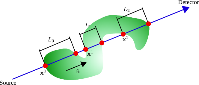
So far we have restricted the model to the case where each neutron beam passes through the sample only once on its way from the source to the detector. In the general case, however, we must allow the beam to pass through several segments of the sample. We denote the starting points of the P𝑃P different segments with 𝐱ksuperscript𝐱𝑘\mathbf{\boldsymbol{\mathrm{x}}}^{k} and the corresponding end points with 𝐱k+Lk𝐧^superscript𝐱𝑘superscript𝐿𝑘^𝐧\mathbf{\boldsymbol{\mathrm{x}}}^{k}+L^{k}\hat{\mathbf{\mathbf{\boldsymbol{\mathrm{n}}}}} as illustrated in Fig. 2. The measurement is still to be interpreted as the average strain tensor along these line segments. Therefore, we have to integrate along all of these line segments and normalise with the total length k=0P1Lksuperscriptsubscript𝑘0𝑃1superscript𝐿𝑘\sum\nolimits_{k=0}^{P-1}L^{k} travelled though the sample. The measurement equation (16) then turns into

I(𝜼)I𝜼\displaystyle\mathrm{I}(\mathbf{\boldsymbol{\mathrm{\eta}}}) =ϑ𝜼[𝐟]=1k=0P1Lkk=0P10Lk𝐧𝖳𝐟(𝐱k+s𝐧^)𝑑s.absentsubscriptbold-italic-ϑ𝜼delimited-[]𝐟1superscriptsubscript𝑘0𝑃1superscript𝐿𝑘superscriptsubscript𝑘0𝑃1superscriptsubscript0superscript𝐿𝑘superscript𝐧𝖳𝐟superscript𝐱𝑘𝑠^𝐧differential-d𝑠\displaystyle=\mathbf{\boldsymbol{\mathrm{\vartheta}}}_{\mathbf{\boldsymbol{\mathrm{\eta}}}}[\mathbf{\boldsymbol{\mathrm{f}}}]=\frac{1}{\sum_{k=0}^{P-1}L^{k}}\sum_{k=0}^{P-1}\int_{0}^{L^{k}}\vec{\mathbf{\boldsymbol{\mathrm{n}}}}^{\mathsf{T}}\mathbf{\boldsymbol{\mathrm{f}}}(\mathbf{\boldsymbol{\mathrm{x}}}^{k}+s\hat{\mathbf{n}})ds. (21)

Here, 𝜼𝜼\mathbf{\boldsymbol{\mathrm{\eta}}} consists of all arguments for all segments 𝜼={𝐱0,L0,,𝐱P1,LP1,𝐧^}𝜼superscript𝐱0superscript𝐿0superscript𝐱𝑃1superscript𝐿𝑃1^𝐧\mathbf{\boldsymbol{\mathrm{\eta}}}=\{\mathbf{\boldsymbol{\mathrm{x}}}^{0},L^{0},\dots,\mathbf{\boldsymbol{\mathrm{x}}}^{P-1},L^{P-1},\hat{\mathbf{\mathbf{\boldsymbol{\mathrm{n}}}}}\}. Note that the direction 𝐧^^𝐧\hat{\mathbf{\mathbf{\boldsymbol{\mathrm{n}}}}} is the same for all segments.

Refer to caption
Figure 2: Illustration of the case where the neutron beam passes through P=3𝑃3P=3 segments of the sample.

Although this modification requires some care in the implementation, there is no conceptual challenge added. The covariance matrices in (19) will change accordingly

(𝐊)isubscriptsubscript𝐊𝑖\displaystyle(\mathbf{\boldsymbol{\mathrm{K}}}_{*})_{i} =1k=0Pi1Likk=0Pi10Lik𝐧i𝖳𝐊(𝐱ik+s𝐧^i,𝐱)𝑑s,absent1superscriptsubscript𝑘0subscript𝑃𝑖1subscriptsuperscript𝐿𝑘𝑖superscriptsubscript𝑘0subscript𝑃𝑖1superscriptsubscript0subscriptsuperscript𝐿𝑘𝑖superscriptsubscript𝐧𝑖𝖳𝐊subscriptsuperscript𝐱𝑘𝑖𝑠subscript^𝐧𝑖subscript𝐱differential-d𝑠\displaystyle=\frac{1}{\sum_{k=0}^{P_{i}-1}L^{k}_{i}}\sum_{k=0}^{P_{i}-1}\int_{0}^{L^{k}_{i}}\vec{\mathbf{\boldsymbol{\mathrm{n}}}}_{i}^{\mathsf{T}}\mathbf{\boldsymbol{\mathrm{K}}}(\mathbf{\boldsymbol{\mathrm{x}}}^{k}_{i}+s\hat{\mathbf{n}}_{i},\mathbf{\boldsymbol{\mathrm{x}}}_{*})ds, (22a)
(𝐊I)ijsubscriptsubscript𝐊I𝑖𝑗\displaystyle(\mathbf{\boldsymbol{\mathrm{K}}}_{\mathrm{I}})_{ij} =1(k=0Pi1Lik)(l=0Pj1Ljl)k=0Pi1l=0Pj1[0Ljl0Lik𝐧i𝖳𝐊(𝐱ik+si𝐧^i,𝐱jl+sj𝐧^j)𝐧j𝑑si𝑑sj].absent1superscriptsubscript𝑘0subscript𝑃𝑖1subscriptsuperscript𝐿𝑘𝑖superscriptsubscript𝑙0subscript𝑃𝑗1subscriptsuperscript𝐿𝑙𝑗superscriptsubscript𝑘0subscript𝑃𝑖1superscriptsubscript𝑙0subscript𝑃𝑗1delimited-[]superscriptsubscript0superscriptsubscript𝐿𝑗𝑙superscriptsubscript0superscriptsubscript𝐿𝑖𝑘superscriptsubscript𝐧𝑖𝖳𝐊subscriptsuperscript𝐱𝑘𝑖subscript𝑠𝑖subscript^𝐧𝑖subscriptsuperscript𝐱𝑙𝑗subscript𝑠𝑗subscript^𝐧𝑗subscript𝐧𝑗differential-dsubscript𝑠𝑖differential-dsubscript𝑠𝑗\displaystyle=\frac{1}{\left(\sum_{k=0}^{P_{i}-1}L^{k}_{i}\right)\left(\sum_{l=0}^{P_{j}-1}L^{l}_{j}\right)}\sum_{k=0}^{P_{i}-1}\sum_{l=0}^{P_{j}-1}\bigg{[}\int_{0}^{L_{j}^{l}}\int_{0}^{L_{i}^{k}}\vec{\mathbf{\boldsymbol{\mathrm{n}}}}_{i}^{\mathsf{T}}\mathbf{\boldsymbol{\mathrm{K}}}(\mathbf{\boldsymbol{\mathrm{x}}}^{k}_{i}+s_{i}\hat{\mathbf{n}}_{i},\mathbf{\boldsymbol{\mathrm{x}}}^{l}_{j}+s_{j}\hat{\mathbf{n}}_{j})\vec{\mathbf{\boldsymbol{\mathrm{n}}}}_{j}ds_{i}ds_{j}\bigg{]}. (22b)

The reconstruction procedure described in (20) remains the same with these new covariance matrices in place.

4 The model in practice

Before presenting the numerical results, we discuss a couple of important practical aspects concerning the computational complexity and the hyperparameter selection. The approach as described below is summarised in Algorithm 1.

4.1 Reducing the computational complexity

A bottleneck in GP regression is the storage and inversion of the matrix 𝐊I+σ2𝐈subscript𝐊Isuperscript𝜎2𝐈\mathbf{\boldsymbol{\mathrm{K}}}_{\mathrm{I}}+\sigma^{2}\mathbf{\boldsymbol{\mathrm{I}}} in (20), which scales as 𝒪(N2)𝒪superscript𝑁2\mathcal{O}(N^{2}) and 𝒪(N3)𝒪superscript𝑁3\mathcal{O}(N^{3}) in memory and time, respectively. For large data sets, approximate methods are motivated by the need to decrease the problem size, making memory requirements manageable and reducing the runtime. There are a variety of methods described in the literature, and we refer to (Quiñonero Candela et al.,, 2007) for a useful review. Here we make use of the approximation method proposed by Solin and Särkkä, (2014), which turns out to fit our model very well. A drawback with this method is that it requires the covariance function to be stationary, which means that it is dependent only on the difference between the input locations. However, that is true for some of the most common ones, including the squared exponential (12).

The key idea is to estimate the covariance function as a truncated sum of m𝑚m basis functions

kφ(𝐱,𝐱)i=1mS(𝝀i)ϕi(𝐱)ϕi(𝐱),subscript𝑘𝜑𝐱superscript𝐱bold-′superscriptsubscript𝑖1𝑚𝑆subscript𝝀𝑖subscriptitalic-ϕ𝑖𝐱subscriptitalic-ϕ𝑖superscript𝐱k_{\varphi}(\mathbf{\boldsymbol{\mathrm{x,x^{\prime}}}})\approx\sum_{i=1}^{m}S(\boldsymbol{\lambda}_{i})\phi_{i}(\mathbf{\boldsymbol{\mathrm{x}}})\phi_{i}(\mathbf{\boldsymbol{\mathrm{x}}}^{\prime}), (23)

where S𝑆S is the spectral density of the covariance function. For a stationary covariance function kφ=kφ(𝒓)subscript𝑘𝜑subscript𝑘𝜑𝒓k_{\varphi}=k_{\varphi}(\boldsymbol{r}) where 𝒓=𝐱𝐱𝒓𝐱superscript𝐱\boldsymbol{r}=\mathbf{\boldsymbol{\mathrm{x}}}-\mathbf{\boldsymbol{\mathrm{x}}}^{\prime}, the spectral density is given by

S(𝝎)=k(𝒓)ei𝝎𝖳𝒓𝑑𝒓.𝑆𝝎𝑘𝒓superscript𝑒isuperscript𝝎𝖳𝒓differential-d𝒓S(\boldsymbol{\omega})=\int k(\boldsymbol{r})e^{-\text{i}\boldsymbol{\omega}^{\mathsf{T}}\boldsymbol{r}}d\boldsymbol{r}. (24)

The basis functions ϕi(𝐱)subscriptitalic-ϕ𝑖𝐱\phi_{i}(\mathbf{\boldsymbol{\mathrm{x}}}) and eigenvalues 𝝀isubscript𝝀𝑖\boldsymbol{\lambda}_{i} are obtained from the solution to the Laplace eigenvalue problem on the domain ΩΩ\Omega

{Δϕi(𝐱)=𝝀i2ϕi(𝐱),ϕi(𝐱)=0,𝐱Ω,𝐱Ω.casesformulae-sequenceΔsubscriptitalic-ϕ𝑖𝐱superscriptdelimited-∥∥subscript𝝀𝑖2subscriptitalic-ϕ𝑖𝐱subscriptitalic-ϕ𝑖𝐱0formulae-sequence𝐱Ω𝐱Ω\displaystyle\begin{cases}\begin{split}-\Delta\phi_{i}(\mathbf{\boldsymbol{\mathrm{x}}})&=\|\boldsymbol{\lambda}_{i}\|^{2}\phi_{i}(\mathbf{\boldsymbol{\mathrm{x}}}),\\ \phi_{i}(\mathbf{\boldsymbol{\mathrm{x}}})&=0,\end{split}\end{cases}\quad\begin{split}\mathbf{\boldsymbol{\mathrm{x}}}&\in\Omega,\\ \mathbf{\boldsymbol{\mathrm{x}}}&\in\partial\Omega.\end{split} (25)

The Dirichlet boundary condition is the most natural choice, although any boundary condition could be chosen. For a two-dimensional domain Ω=[ρx,ρx]×[ρy,ρy]Ωsubscript𝜌𝑥subscript𝜌𝑥subscript𝜌𝑦subscript𝜌𝑦\Omega=[-\rho_{x},\rho_{x}]\times[-\rho_{y},\rho_{y}], the solution of (25) reads

ϕi(𝐱)subscriptitalic-ϕ𝑖𝐱\displaystyle\phi_{i}(\mathbf{\boldsymbol{\mathrm{x}}}) =1ρxρysin(λix(x+ρx))sin(λiy(y+ρy)),absent1subscript𝜌𝑥subscript𝜌𝑦subscript𝜆subscript𝑖𝑥𝑥subscript𝜌𝑥subscript𝜆subscript𝑖𝑦𝑦subscript𝜌𝑦\displaystyle=\frac{1}{\sqrt{\rho_{x}\rho_{y}}}\sin\big{(}\lambda_{i_{x}}(x+\rho_{x})\big{)}\sin\big{(}\lambda_{i_{y}}(y+\rho_{y})\big{)}, (26a)
λixsubscript𝜆subscript𝑖𝑥\displaystyle\lambda_{i_{x}} =πix2ρx,λiy=πiy2ρy,formulae-sequenceabsent𝜋subscript𝑖𝑥2subscript𝜌𝑥subscript𝜆subscript𝑖𝑦𝜋subscript𝑖𝑦2subscript𝜌𝑦\displaystyle=\frac{\pi i_{x}}{2\rho_{x}},\qquad\lambda_{i_{y}}=\frac{\pi i_{y}}{2\rho_{y}}, (26b)

where ixsubscript𝑖𝑥i_{x} and iysubscript𝑖𝑦i_{y} are chosen such that the eigenvalues lie in a desired frequency domain, and the size of ΩΩ\Omega should be adjusted thereafter. Loosely speaking, the choice of ρxsubscript𝜌𝑥\rho_{x} determines the frequency resolution in the x𝑥x-direction, and similarly for y𝑦y.

The approximate posterior expressions are

𝔼[f]𝔼delimited-[]subscript𝑓\displaystyle\mathbb{E}[f_{*}] ϕ𝖳(𝚽𝚽𝖳+σ2𝚲1)1𝚽𝐲,absentsuperscriptsubscriptbold-italic-ϕ𝖳superscript𝚽superscript𝚽𝖳superscript𝜎2superscript𝚲11𝚽𝐲\displaystyle\approx\mathbf{\boldsymbol{\mathrm{\phi}}}_{*}^{\mathsf{T}}(\mathbf{\boldsymbol{\mathrm{\Phi}}}\mathbf{\boldsymbol{\mathrm{\Phi}}}^{\mathsf{T}}+\sigma^{2}\mathbf{\boldsymbol{\mathrm{\Lambda}}}^{-1})^{-1}\mathbf{\boldsymbol{\mathrm{\Phi}}}\mathbf{\boldsymbol{\mathrm{y}}}, (27a)
𝕍[f]𝕍delimited-[]subscript𝑓\displaystyle\mathbb{V}[f_{*}] σ2ϕ𝖳(𝚽𝚽𝖳+σ2𝚲1)1ϕ,absentsuperscript𝜎2superscriptsubscriptbold-italic-ϕ𝖳superscript𝚽superscript𝚽𝖳superscript𝜎2superscript𝚲11subscriptbold-italic-ϕ\displaystyle\approx\sigma^{2}\mathbf{\boldsymbol{\mathrm{\phi}}}_{*}^{\mathsf{T}}(\mathbf{\boldsymbol{\mathrm{\Phi}}}\mathbf{\boldsymbol{\mathrm{\Phi}}}^{\mathsf{T}}+\sigma^{2}\mathbf{\boldsymbol{\mathrm{\Lambda}}}^{-1})^{-1}\mathbf{\boldsymbol{\mathrm{\phi}}}_{*}, (27b)

where 𝚽ij=ϕi(𝐱j)subscript𝚽𝑖𝑗subscriptitalic-ϕ𝑖subscript𝐱𝑗\boldsymbol{\Phi}_{ij}=\phi_{i}(\mathbf{\boldsymbol{\mathrm{x}}}_{j}), ϕ=[ϕ1(𝐱)ϕm(𝐱)]𝖳subscriptbold-italic-ϕsuperscriptdelimited-[]subscriptitalic-ϕ1subscript𝐱subscriptitalic-ϕ𝑚subscript𝐱𝖳\mathbf{\boldsymbol{\mathrm{\phi}}}_{*}=[\phi_{1}(\mathbf{\boldsymbol{\mathrm{x}}}_{*})\dots\phi_{m}(\mathbf{\boldsymbol{\mathrm{x}}}_{*})]^{\mathsf{T}} and 𝚲jj=S(𝝀j)subscript𝚲𝑗𝑗𝑆subscript𝝀𝑗\boldsymbol{\Lambda}_{jj}=S(\boldsymbol{\lambda}_{j}). The correct expressions for our problem are found by projecting the transformation given by (16) onto the basis functions. We end up with

𝔼[𝐟]𝔼delimited-[]subscript𝐟\displaystyle\mathbb{E}[\mathbf{\boldsymbol{\mathrm{f}}}_{*}] 𝐐𝖳(𝐐𝐐𝖳+σ2𝚲1)1𝐐𝐲,absentsuperscriptsubscript𝐐𝖳superscriptsuperscript𝐐𝐐𝖳superscript𝜎2superscript𝚲11𝐐𝐲\displaystyle\approx\mathbf{\boldsymbol{\mathrm{Q}}}_{*}^{\mathsf{T}}(\mathbf{\boldsymbol{\mathrm{Q}}}\mathbf{\boldsymbol{\mathrm{Q}}}^{\mathsf{T}}+\sigma^{2}\mathbf{\boldsymbol{\mathrm{\Lambda}}}^{-1})^{-1}\mathbf{\boldsymbol{\mathrm{Q}}}\mathbf{\boldsymbol{\mathrm{y}}}, (28a)
𝕍[𝐟]𝕍delimited-[]subscript𝐟\displaystyle\mathbb{V}[\mathbf{\boldsymbol{\mathrm{f}}}_{*}] σ2𝐐𝖳(𝐐𝐐𝖳+σ2𝚲1)1𝐐.absentsuperscript𝜎2superscriptsubscript𝐐𝖳superscriptsuperscript𝐐𝐐𝖳superscript𝜎2superscript𝚲11subscript𝐐\displaystyle\approx\sigma^{2}\mathbf{\boldsymbol{\mathrm{Q}}}_{*}^{\mathsf{T}}(\mathbf{\boldsymbol{\mathrm{Q}}}\mathbf{\boldsymbol{\mathrm{Q}}}^{\mathsf{T}}+\sigma^{2}\mathbf{\boldsymbol{\mathrm{\Lambda}}}^{-1})^{-1}\mathbf{\boldsymbol{\mathrm{Q}}}_{*}. (28b)

where

𝐐subscript𝐐\displaystyle\mathbf{\boldsymbol{\mathrm{Q}}}_{*} =[𝐱ϕ1|𝐱=𝐱𝐱ϕm|𝐱=𝐱]𝖳,absentsuperscriptmatrixevaluated-atsubscript𝐱subscriptitalic-ϕ1𝐱subscript𝐱evaluated-atsubscript𝐱subscriptitalic-ϕ𝑚𝐱subscript𝐱𝖳\displaystyle=\begin{bmatrix}\mathcal{L}_{\mathbf{\boldsymbol{\mathrm{x}}}}\phi_{1}|_{\mathbf{\boldsymbol{\mathrm{x}}}=\mathbf{\boldsymbol{\mathrm{x}}}_{*}}&\dots&\mathcal{L}_{\mathbf{\boldsymbol{\mathrm{x}}}}\phi_{m}|_{\mathbf{\boldsymbol{\mathrm{x}}}=\mathbf{\boldsymbol{\mathrm{x}}}_{*}}\end{bmatrix}^{\mathsf{T}}, (29a)
𝐐ijsubscript𝐐𝑖𝑗\displaystyle\mathbf{\boldsymbol{\mathrm{Q}}}_{ij} =ϑ𝜼j[𝐱ϕi].absentsubscriptbold-italic-ϑsubscript𝜼𝑗delimited-[]subscript𝐱subscriptitalic-ϕ𝑖\displaystyle=\mathbf{\boldsymbol{\mathrm{\vartheta}}}_{\mathbf{\boldsymbol{\mathrm{\eta}}}_{j}}[\mathcal{L}_{\mathbf{\boldsymbol{\mathrm{x}}}}\phi_{i}]. (29b)

Comparing this with (22), we have used that 𝐊𝐐𝖳𝚲𝐐subscript𝐊superscript𝐐𝖳𝚲subscript𝐐\mathbf{\boldsymbol{\mathrm{K}}}_{*}\approx\mathbf{\boldsymbol{\mathrm{Q}}}^{\mathsf{T}}\boldsymbol{\Lambda}\mathbf{\boldsymbol{\mathrm{Q}}}_{*} and 𝐊I𝐐𝖳𝚲𝐐subscript𝐊Isuperscript𝐐𝖳𝚲𝐐\mathbf{\boldsymbol{\mathrm{K}}}_{\mathrm{I}}\approx\mathbf{\boldsymbol{\mathrm{Q}}}^{\mathsf{T}}\boldsymbol{\Lambda}\mathbf{\boldsymbol{\mathrm{Q}}}, and the computationally more preferable form (29) is obtained by utilising the identities

𝐏𝐁𝖳(𝐁𝐏𝐁𝖳+𝐑)1=(𝐁𝖳𝐑1𝐁+𝐏1)1𝐁𝖳𝐑1,superscript𝐏𝐁𝖳superscriptsuperscript𝐁𝐏𝐁𝖳𝐑1superscriptsuperscript𝐁𝖳superscript𝐑1𝐁superscript𝐏11superscript𝐁𝖳superscript𝐑1\displaystyle\mathbf{\boldsymbol{\mathrm{P}}}\mathbf{\boldsymbol{\mathrm{B}}}^{\mathsf{T}}(\mathbf{\boldsymbol{\mathrm{B}}}\mathbf{\boldsymbol{\mathrm{P}}}\mathbf{\boldsymbol{\mathrm{B}}}^{\mathsf{T}}+\mathbf{\boldsymbol{\mathrm{R}}})^{-1}=(\mathbf{\boldsymbol{\mathrm{B}}}^{\mathsf{T}}\mathbf{\boldsymbol{\mathrm{R}}}^{-1}\mathbf{\boldsymbol{\mathrm{B}}}+\mathbf{\boldsymbol{\mathrm{P}}}^{-1})^{-1}\mathbf{\boldsymbol{\mathrm{B}}}^{\mathsf{T}}\mathbf{\boldsymbol{\mathrm{R}}}^{-1},
and
𝐀𝐀𝐂𝖳(𝐂𝐀𝐂𝖳+𝐖)1𝐂𝐀=(𝐂𝖳𝐖1𝐂+𝐀1)1.𝐀superscript𝐀𝐂𝖳superscriptsuperscript𝐂𝐀𝐂𝖳𝐖1𝐂𝐀superscriptsuperscript𝐂𝖳superscript𝐖1𝐂superscript𝐀11\displaystyle\mathbf{\boldsymbol{\mathrm{A}}}-\mathbf{\boldsymbol{\mathrm{A}}}\mathbf{\boldsymbol{\mathrm{C}}}^{\mathsf{T}}(\mathbf{\boldsymbol{\mathrm{C}}}\mathbf{\boldsymbol{\mathrm{A}}}\mathbf{\boldsymbol{\mathrm{C}}}^{\mathsf{T}}+\mathbf{\boldsymbol{\mathrm{W}}})^{-1}\mathbf{\boldsymbol{\mathrm{C}}}\mathbf{\boldsymbol{\mathrm{A}}}=(\mathbf{\boldsymbol{\mathrm{C}}}^{\mathsf{T}}\mathbf{\boldsymbol{\mathrm{W}}}^{-1}\mathbf{\boldsymbol{\mathrm{C}}}+\mathbf{\boldsymbol{\mathrm{A}}}^{-1})^{-1}.

This approximation scheme reduces the complexity of the regression from 𝒪(N3)𝒪superscript𝑁3\mathcal{O}(N^{3}) to 𝒪(Nm2)𝒪𝑁superscript𝑚2\mathcal{O}(Nm^{2}). The actual savings in our case are even larger, since the hazard of numerically computing the integrals in (22) is removed: now all we need is to compute single integrals, and this is done analytically due to the simple form of the basis functions (for details see D). Hence, for this particular problem, the approximation is computationally preferable even if N<m𝑁𝑚N<m.

Extending to multiple test points {𝐱j}j=1Msuperscriptsubscriptsuperscriptsubscript𝐱𝑗𝑗1𝑀\{\mathbf{\boldsymbol{\mathrm{x}}}_{*}^{j}\}_{j=1}^{M}, all we need to change is 𝐐subscript𝐐\mathbf{\boldsymbol{\mathrm{Q}}}_{*}, so that (29a) becomes

𝐐subscript𝐐\displaystyle\mathbf{\boldsymbol{\mathrm{Q}}}_{*} =[𝐱ϕ1|𝐱=𝐱1𝐱ϕm|𝐱=𝐱1𝐱ϕ1|𝐱=𝐱M𝐱ϕm|𝐱=𝐱M]𝖳.absentsuperscriptmatrixevaluated-atsubscript𝐱subscriptitalic-ϕ1𝐱superscriptsubscript𝐱1evaluated-atsubscript𝐱subscriptitalic-ϕ𝑚𝐱superscriptsubscript𝐱1evaluated-atsubscript𝐱subscriptitalic-ϕ1𝐱superscriptsubscript𝐱𝑀evaluated-atsubscript𝐱subscriptitalic-ϕ𝑚𝐱superscriptsubscript𝐱𝑀𝖳\displaystyle=\begin{bmatrix}\mathcal{L}_{\mathbf{\boldsymbol{\mathrm{x}}}}\phi_{1}|_{\mathbf{\boldsymbol{\mathrm{x}}}=\mathbf{\boldsymbol{\mathrm{x}}}_{*}^{1}}&\dots&\mathcal{L}_{\mathbf{\boldsymbol{\mathrm{x}}}}\phi_{m}|_{\mathbf{\boldsymbol{\mathrm{x}}}=\mathbf{\boldsymbol{\mathrm{x}}}_{*}^{1}}\\ \vdots&\vdots&\vdots\\ \mathcal{L}_{\mathbf{\boldsymbol{\mathrm{x}}}}\phi_{1}|_{\mathbf{\boldsymbol{\mathrm{x}}}=\mathbf{\boldsymbol{\mathrm{x}}}_{*}^{M}}&\dots&\mathcal{L}_{\mathbf{\boldsymbol{\mathrm{x}}}}\phi_{m}|_{\mathbf{\boldsymbol{\mathrm{x}}}=\mathbf{\boldsymbol{\mathrm{x}}}_{*}^{M}}\end{bmatrix}^{\mathsf{T}}. (30)

The expressions (28) are then applied as before. Note that, usually what is desired is the variance of the different component values in each test point, and not the covariance between them. Hence, we should not compute the entire matrix in (28b), but only its diagonal elements.

4.2 Hyperparameters

The covariance function kφsubscript𝑘𝜑k_{\varphi} is characterised by its hyperparameters 𝜽={θk}𝜽subscript𝜃𝑘\boldsymbol{\theta}=\{\theta_{k}\}. An example was given in equation (12). This set does also include the noise level σ𝜎\sigma. Usually they are selected by maximising the marginal likelihood p(𝐲|{𝜼i},𝜽)𝑝conditional𝐲subscript𝜼𝑖𝜽p(\mathbf{\boldsymbol{\mathrm{y}}}|\{\boldsymbol{\eta}_{i}\},\boldsymbol{\theta}), which is the probability of the data conditioned on the input locations and the hyperparameters. The idea is to choose the hyperparameters 𝜽subscript𝜽\boldsymbol{\theta}_{*} that given the choice of covariance function are most likely to have generated the observed data. The marginal likelihood and its derivatives can be computed in closed form (Rasmussen and Williams,, 2006). For convenience, the logarithm of the marginal likelihood is usually considered, and it is for our problem given by

logp(𝐲|{𝜼i},𝜽)=12logdet(𝐊I+σ2I)12𝐲𝖳(𝐊I+σ2I)1𝐲N2log2π,𝑝conditional𝐲subscript𝜼𝑖𝜽12subscript𝐊Isuperscript𝜎2𝐼12superscript𝐲𝖳superscriptsubscript𝐊Isuperscript𝜎2𝐼1𝐲𝑁22𝜋\displaystyle\log p(\mathbf{\boldsymbol{\mathrm{y}}}|\{\boldsymbol{\eta}_{i}\},\boldsymbol{\theta})=-\frac{1}{2}\log\det(\mathbf{\boldsymbol{\mathrm{K}}}_{\mathrm{I}}+\sigma^{2}I)-\frac{1}{2}\mathbf{\boldsymbol{\mathrm{y}}}^{\mathsf{T}}(\mathbf{\boldsymbol{\mathrm{K}}}_{\mathrm{I}}+\sigma^{2}I)^{-1}\mathbf{\boldsymbol{\mathrm{y}}}-\frac{N}{2}\log 2\pi, (31)

where 𝐊Isubscript𝐊I\mathbf{\boldsymbol{\mathrm{K}}}_{\mathrm{I}} is a function of 𝜽𝜽\boldsymbol{\theta}. Since the constant term is irrelevant for optimisation purposes, we get

𝜽=argmax𝜽[12logdet(𝐊I+σ2I)12𝐲𝖳(𝐊I+σ2I)1𝐲].subscript𝜽𝜽argmaxdelimited-[]12subscript𝐊Isuperscript𝜎2𝐼12superscript𝐲𝖳superscriptsubscript𝐊Isuperscript𝜎2𝐼1𝐲\displaystyle\boldsymbol{\theta}_{*}=\underset{\boldsymbol{\theta}}{\text{argmax}}\Big{[}-\frac{1}{2}\log\det(\mathbf{\boldsymbol{\mathrm{K}}}_{\mathrm{I}}+\sigma^{2}I)-\frac{1}{2}\mathbf{\boldsymbol{\mathrm{y}}}^{\mathsf{T}}(\mathbf{\boldsymbol{\mathrm{K}}}_{\mathrm{I}}+\sigma^{2}I)^{-1}\mathbf{\boldsymbol{\mathrm{y}}}\Big{]}. (32)

An approximative version of (32) is obtained by replacing 𝐊Isubscript𝐊I\mathbf{\boldsymbol{\mathrm{K}}}_{\mathrm{I}} with 𝐐𝖳𝚲𝐐superscript𝐐𝖳𝚲𝐐\mathbf{\boldsymbol{\mathrm{Q}}}^{\mathsf{T}}\boldsymbol{\Lambda}\mathbf{\boldsymbol{\mathrm{Q}}}. The derivative expressions for this case are given in D.2. The optimisation can thereafter be carried out using any standard gradient-based method, such as for example the BFGS algorithm (Nocedal and Wright,, 2000).

Algorithm 1 Reconstructing the GP with the reduced-rank approach
0:  𝒟={(𝜼i,yi)}i=1N𝒟superscriptsubscriptsubscript𝜼𝑖subscript𝑦𝑖𝑖1𝑁\mathcal{D}=\{(\mathbf{\boldsymbol{\mathrm{\eta}}}_{i},y_{i})\}_{i=1}^{N}, 𝐱subscript𝐱\mathbf{\boldsymbol{\mathrm{x}}}_{*}, ΩΩ\Omega, m𝑚m.
0:  𝔼[𝐟(𝐱)],𝕍[𝐟(𝐱)]𝔼delimited-[]𝐟subscript𝐱𝕍delimited-[]𝐟subscript𝐱\mathbb{E}[\mathbf{\boldsymbol{\mathrm{f}}}(\mathbf{\boldsymbol{\mathrm{x}}}_{*})],\mathbb{V}[\mathbf{\boldsymbol{\mathrm{f}}}(\mathbf{\boldsymbol{\mathrm{x}}}_{*})].
1:  Construct the matrix 𝐐𝐐\mathbf{\boldsymbol{\mathrm{Q}}} as defined in (29b), with details given in D.
2:  Optimise the hyperparameters 𝜽𝜽\mathbf{\boldsymbol{\mathrm{\theta}}} as described in Section 4.2.
3:  Construct 𝐐subscript𝐐\mathbf{\boldsymbol{\mathrm{Q}}}_{*} as defined in (29a).
4:  Solve the GP regression problem by (28).

5 Experimental results

5.1 Simulated experiment – cantilevered rectangular plate

As a simple example illustrating the potential of the method, consider the problem presented in (Wensrich et al., 2016a, ). A cantilevered plate is subject to a vertical load at the right end, see Fig. 3. The approximate equations for the strain field components are

ϵxxsubscriptitalic-ϵ𝑥𝑥\displaystyle\epsilon_{xx} =PEI(lx)y,absent𝑃𝐸𝐼𝑙𝑥𝑦\displaystyle=\frac{P}{EI}(l-x)y, (33a)
ϵxysubscriptitalic-ϵ𝑥𝑦\displaystyle\epsilon_{xy} =(1+ν)P2EI(h24y2),absent1𝜈𝑃2𝐸𝐼superscript24superscript𝑦2\displaystyle=-\frac{(1+\nu)P}{2EI}\left(\frac{h^{2}}{4}-y^{2}\right), (33b)
ϵyysubscriptitalic-ϵ𝑦𝑦\displaystyle\epsilon_{yy} =νPEI(lx)y,absent𝜈𝑃𝐸𝐼𝑙𝑥𝑦\displaystyle=-\frac{\nu P}{EI}(l-x)y, (33c)

where I=th3/12𝐼𝑡superscript312I=th^{3}/12. Here, I𝐼I denotes the moment of inertia, l𝑙l, hh, and t𝑡t denotes the width, height and thickness of the plate, P𝑃P denotes the magnitude of the load and E𝐸E and ν𝜈\nu denote Youngs modulus and Poisson’s ratio, respectively. We are using the same numerical values as in (Wensrich et al., 2016a, ), namely E=200 GPa𝐸times200gigapascalE=$200\text{\,}\mathrm{GPa}$, ν=0.3𝜈0.3\nu=0.3, h=10 mmtimes10millimeterh=$10\text{\,}\mathrm{mm}$, t=6 mm𝑡times6millimetert=$6\text{\,}\mathrm{mm}$, l=20 mm𝑙times20millimeterl=$20\text{\,}\mathrm{mm}$ and P=2 kN𝑃times2kilonewtonP=$2\text{\,}\mathrm{kN}$. The standard deviation of the synthetic measurement noise is here σ=106𝜎superscript106\sigma=10^{-6}, which was found suitable for illustration purpose. The covariance function used was constructed as described in Section 3.2 with kφ(𝐱,𝐱)=exp(𝐱𝐱)subscript𝑘𝜑𝐱superscript𝐱norm𝐱superscript𝐱k_{\varphi}(\mathbf{\boldsymbol{\mathrm{x}}},\mathbf{\boldsymbol{\mathrm{x}}}^{\prime})=\exp(-\|\mathbf{\boldsymbol{\mathrm{x}}}-\mathbf{\boldsymbol{\mathrm{x}}}^{\prime}\|).

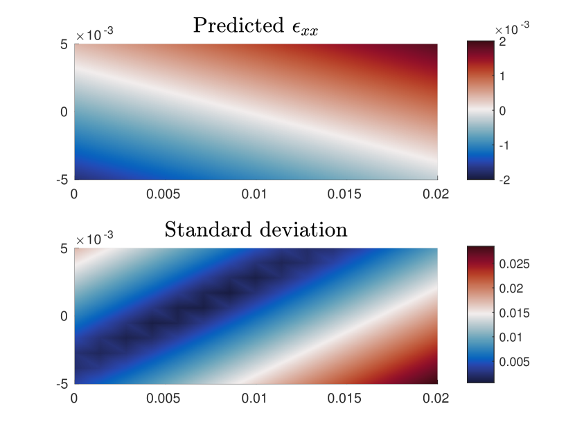
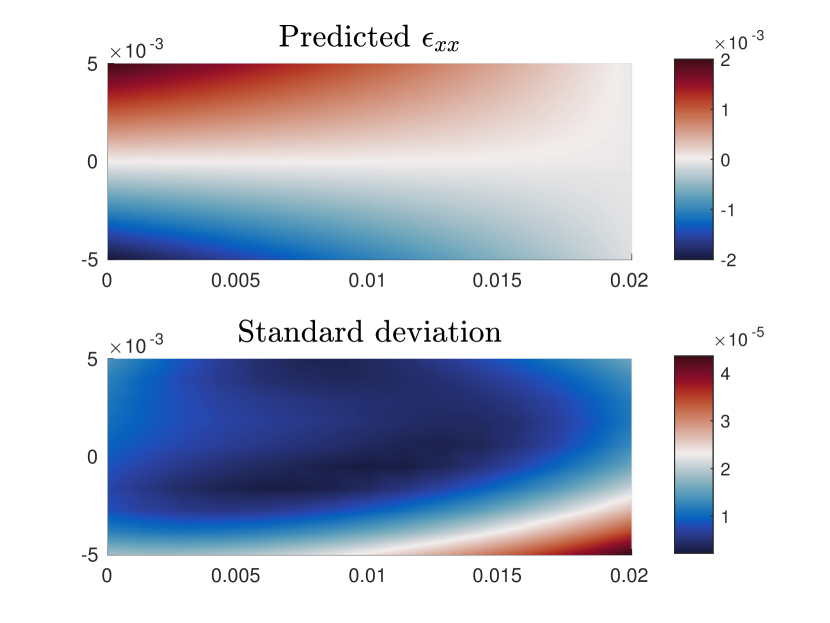
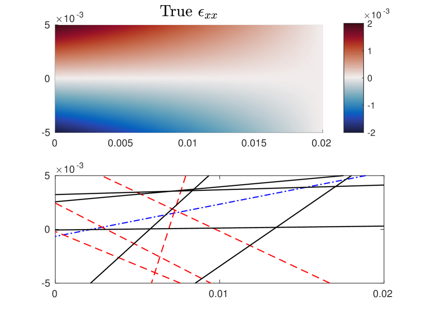
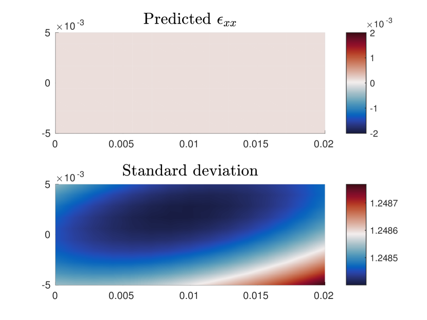
The ϵxxsubscriptitalic-ϵ𝑥𝑥\epsilon_{xx}-component according to (33a) is illustrated in Fig. 4(a) together with the paths along which the line integral (16) have been generated. The remaining three figures in Fig. 4 show the reconstructed component and its standard deviation using 1, 5 and 10 measurements, respectively.

The reconstruction was made by building the matrices defined in (19), and then applying (20b). It is interesting to note that only 10 measurements are enough for the method to produce a reconstruction that is very hard to visually distinguish from the true function. Note that the uncertainty is higher in regions further away from the measurements.
hhl𝑙ly𝑦yx𝑥xP𝑃Py𝑦yz𝑧zt𝑡t
Figure 3: Rectangular plate of width l𝑙l, height hh and thickness t𝑡t, cantilevered on the left side and subject to a vertical load P𝑃P on the right. The approximate strain components within this plate are given by (33).


Refer to caption
(a) True component and 10 line integral measurements, number 1 (blue dashed-dot), 2-5 (red dashed), 6-10 (black solid).
Refer to caption
(b) Prediction (top) and its standard deviation (bottom) after the first measurement (blue dashed-dot line).
Refer to caption
(c) Prediction (top) and its standard deviation (bottom) after 5 measurements (blue dashed-dot line and red dashed lines).
Refer to caption
(d) Prediction (top) and its standard deviation (bottom) after all measurements.
Figure 4: True and reconstructed strain field including its standard deviation for the ϵxxsubscriptitalic-ϵ𝑥𝑥\epsilon_{xx}-component in the rectangular plate shown in Fig. 3. The measurements are the line integral paths shown in the top left figure. Note that the uncertainty is larger at the regions that are poorly covered by the measurements.

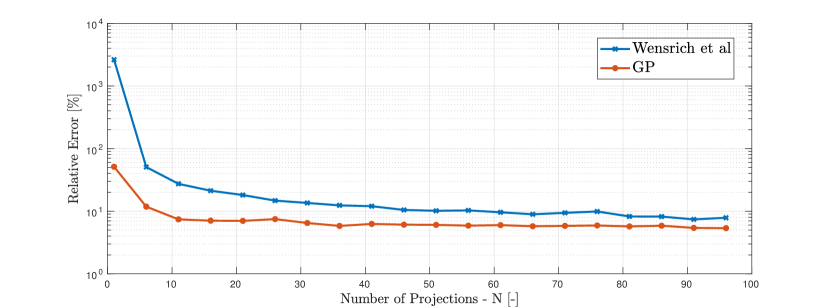
For comparison, we are performing a convergence study similar to the one performed by Wensrich et al., 2016a . Here, the measured data is not generated using (33) but instead from a finite element solution of the problem, which should better reflect reality. To line up with the real experimental setting, the data is not randomly chosen but comes in chunks corresponding to different projections. Each projection typically contains a couple of hundred measurements taken from the same angle but uniformly distributed along the perpendicular direction.

We consider the synthetic noise level σ=104𝜎superscript104\sigma=10^{-4}, to align with Wensrich et al., 2016a where that value was used as an expected experimental measurement noise level. To model the Airy stress function, we are here using the Matérn5/2 covariance function

kφ(𝐱,𝐱)subscript𝑘𝜑𝐱superscript𝐱\displaystyle k_{\varphi}(\mathbf{\boldsymbol{\mathrm{x}}},\mathbf{\boldsymbol{\mathrm{x}}}^{\prime}) =σf2(1+5r~+53r~2)e5r~,absentsuperscriptsubscript𝜎𝑓215~𝑟53superscript~𝑟2superscript𝑒5~𝑟\displaystyle=\sigma_{f}^{2}\left(1+\sqrt{5}\tilde{r}+\frac{5}{3}\tilde{r}^{2}\right)e^{-\sqrt{5}\tilde{r}}, (34a)
r~2superscript~𝑟2\displaystyle\tilde{r}^{2} =lx2(xx)2+ly2(yy)2,absentsuperscriptsubscript𝑙𝑥2superscript𝑥superscript𝑥2superscriptsubscript𝑙𝑦2superscript𝑦superscript𝑦2\displaystyle=l_{x}^{-2}(x-x^{\prime})^{2}+l_{y}^{-2}(y-y^{\prime})^{2}, (34b)

with the hyperparameters chosen by maximising the marginal likelihood (32). This covariance function belongs to a generalisation that relaxes the extreme smoothness assumptions of the squared exponential covariance function (12), and is often considered to be somewhat more realistic. The prediction is made in uniformly distributed points on a 40×20402040\times 20 mesh.

We are reporting the relative error in the reconstruction, where this involves a concatenation of all components in all points. For a total set of N𝑁N projections, the angle from which projection k𝑘k is taken has been chosen as π96+95k1N10.5π96𝜋9695𝑘1𝑁10.5𝜋96\frac{\pi}{96}+\lceil 95\frac{k-1}{N-1}-0.5\rceil\frac{\pi}{96}, so the projection angles are approximately evenly spaced over [0,π]0𝜋[0,\,\,\pi]. Gaussian noise has been added to the measurements with Matlab:s default random seed.

We have here used the approximative method described in Section 4.1 with ρx=3lsubscript𝜌𝑥3𝑙\rho_{x}=3l, ρy=3h/2subscript𝜌𝑦32\rho_{y}=3h/2 and a total number of 160 basis functions. The spectral density of the Matérn5/2 covariance function (34a) is given by

S(𝝎)=σf21005πlxly(5+lx2ωx2+ly2ωy2)7/2Γ(7/2)Γ(5/2),𝑆𝝎superscriptsubscript𝜎𝑓21005𝜋subscript𝑙𝑥subscript𝑙𝑦superscript5superscriptsubscript𝑙𝑥2superscriptsubscript𝜔𝑥2superscriptsubscript𝑙𝑦2superscriptsubscript𝜔𝑦272Γ72Γ52S(\boldsymbol{\omega})=\sigma_{f}^{2}100\sqrt{5}\pi l_{x}l_{y}(5+l_{x}^{2}\omega_{x}^{2}+l_{y}^{2}\omega_{y}^{2})^{-7/2}\frac{\Gamma(7/2)}{\Gamma(5/2)}, (35)

where Γ()Γ\Gamma(\cdot) is the gamma function.

The result is shown in Fig. 5, which also contains the corresponding curve from (Wensrich et al., 2016a, ) for comparison.
Refer to caption
Figure 5: Relative error in the GP-reconstruction as a function of the number of projections.

It is seen that the GP-reconstruction is more accurate and requires less measurements to achieve an equivalent performance.

5.2 Real data

In this section we are solving the problem using data collected from a real-world experiment at the Japan Proton Research Accelerator Complex (JPARC). A brief description of the experimental settings is given below, and we refer to Hendriks et al., (2017) for details.

The sample considered is a thin C-shaped steel plate subject to a compressive load of roughly 7 kNtimes7kN7\text{\,}\mathrm{k}\mathrm{N}. In polar coordinates it is defined by rin=3.5 mm<r<rout=10 mmsubscript𝑟intimes3.5mm𝑟subscript𝑟outtimes10mmr_{\text{in}}=$3.5\text{\,}\mathrm{m}\mathrm{m}$<r<r_{\text{out}}=$10\text{\,}\mathrm{m}\mathrm{m}$ and 45 °<θ<315 °times45degree𝜃times315degree$45\text{\,}\mathrm{\SIUnitSymbolDegree}$<\theta<$315\text{\,}\mathrm{\SIUnitSymbolDegree}$.

The data set consists of 86 projections taken from evenly distributed angles around the sample. The experimental resolution of the detector is 512x512. Since this particular experiment was dealing with a planar strain field the detector pixels could be grouped by column (in the out of plane direction) to improve the statistics, giving a possible 512 measurements per projection. However, due to the sample size and shape not all rays would have passed through the sample. On average roughly 350 measurements were made per projection, giving a total amount of nearly 30 000 measurements. It should be noted that the sample took up slightly less than half the detectors height (as another sample was also being analysed) and so about 200 pixels were binned for each measurement.

The Matérn5/2 covariance function (34a) was used, and for the approximate settings we have taken ρx=ρy=2.5routsubscript𝜌𝑥subscript𝜌𝑦2.5subscript𝑟out\rho_{x}=\rho_{y}=2.5r_{\text{out}} and a total number of 673 basis functions.

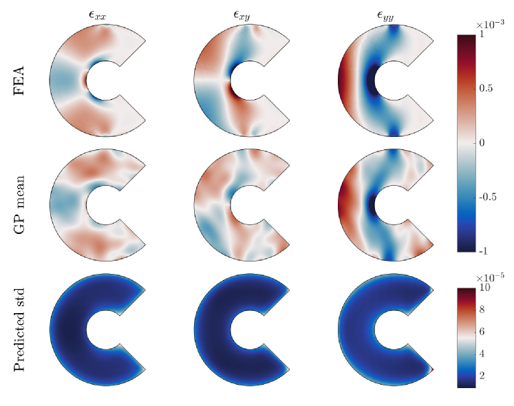
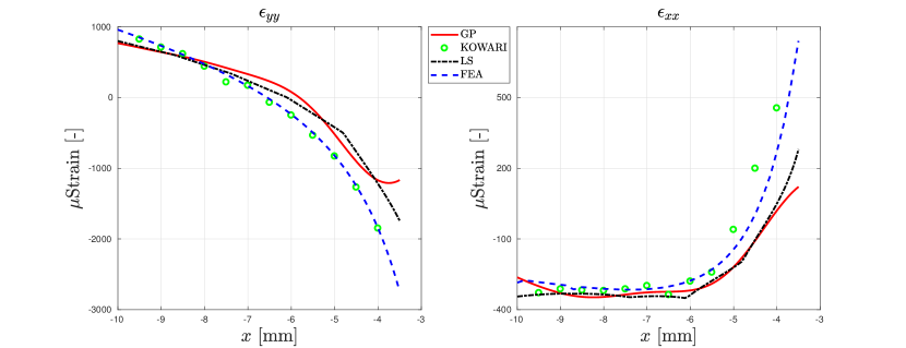
The result is shown in Fig. 6. The top row shows a finite element solution to the simulated problem, while the middle and bottom rows contains the mean and standard deviation of the GP reconstruction. Fig. 7 is showing the ϵyysubscriptitalic-ϵ𝑦𝑦\epsilon_{yy}- and ϵxxsubscriptitalic-ϵ𝑥𝑥\epsilon_{xx}-components along the line y=0𝑦0y=0. The data points labelled KOWARI emerges from a constant wavelength scanning experiment, which is a well established method for accurate measurement of average strain within a gauge volume (Hendriks et al.,, 2017). Also, LS denote the reconstruction obtained from the least squares approach used by Hendriks et al., (2017).

Although the GP reconstruction follows the overall structure of the FEA solution and the KOWARI data, there are regions of notable deviations. This is particularly clear at the right sides in Figure 7, near the boundary of the sample. It has been observed that this deviating behaviour is present when the reconstruction is made from simulated data as well. The boundary challenges are intuitively understood from the nature of the model. From the GP’s perspective, the inferred function is a continuous object, and the natural problem boundary of the sample is not built into the model. Outside the sample the reconstruction will fall back to the prior mean, which obviously has a higher impact on the boundary than on the interior. This effect gives rise to a perceived non-smooth feature, which is hard to capture with the relatively smooth covariance function provided by Matérn5/2.

Moreover, it is not obvious what settings to choose for the approximation method. In theory, the approximation improves as the number of basis functions is increased. In practice, too many basis functions entails numerical problems, while too few gives a poor approximation. This trade-off requires a somehow ad hoc user selection and the precise impact on the solution is hard to anticipate.

Data-specific error sources related to the collection and processing of the raw data are discussed more thoroughly by Hendriks et al., (2017). For example, certain ray paths are short relative to others, and the Bragg-edge estimate hence becomes less accurate in these cases. See Vogel, (2000) for more discussions on systematic error sources in this context.
Refer to caption
Figure 6: Top row: simulated solution obtained through finite element analysis. Middle and bottom row: mean and standard deviation of the GP reconstruction.
Refer to caption
Figure 7: Plots of the GP reconstruction along the line y=0𝑦0y=0, compared to constant wavelength scanning (KOWARI), a finite element simulation (FEA) and a reconstruction obtained through the least squares approach (LS).

6 Concluding remarks

6.1 Compatibility constraint

If the strain field can be expressed as emerging from a continuous, single-valued displacement field, then it is called compatible. Compatibility can be expressed as the linear constraint

[2y22xy2x2]𝓕𝐱C𝐟=0.subscriptmatrixsuperscript2superscript𝑦2superscript2𝑥𝑦superscript2superscript𝑥2superscriptsubscript𝓕𝐱𝐶𝐟0\underbrace{\begin{bmatrix}\frac{\partial^{2}}{\partial y^{2}}&-\frac{\partial^{2}}{\partial x\partial y}&\frac{\partial^{2}}{\partial x^{2}}\end{bmatrix}}_{\mathbf{\boldsymbol{\mathrm{\mathscr{F}}}}_{\mathbf{\boldsymbol{\mathrm{x}}}}^{C}}\mathbf{\boldsymbol{\mathrm{f}}}=0.

If we would like to construct a model with this constraint imposed as well, the scalar function φ(𝐱)𝜑𝐱\varphi(\mathbf{\boldsymbol{\mathrm{x}}}) can no longer be chosen arbitrary. Instead it will be governed by the relation

𝓕𝐱C𝐱φ=0,superscriptsubscript𝓕𝐱𝐶subscript𝐱𝜑0\mathbf{\boldsymbol{\mathrm{\mathscr{F}}}}_{\mathbf{\boldsymbol{\mathrm{x}}}}^{C}\mathcal{L}_{\mathbf{\boldsymbol{\mathrm{x}}}}\varphi=0, (36)

where 𝐱subscript𝐱\mathcal{L}_{\mathbf{\boldsymbol{\mathrm{x}}}} is given by (8). This is the strain formulation of the biharmonic equation, with solutions called biharmonic functions. As shown by Sadd, (2005), separation of variables can be used to express a general solution φsuperscript𝜑\varphi^{*}, where the specific form is determined by the boundary conditions of the problem, and so is the number of parameters.

This gives rise to at least two questions. Firstly, if there is a parametric form of the solution, why would we use a non-parametric regression method? The answer is that a parametric model require the exact form of the solution so that the number of parameters to be estimated is known. This can only be done provided accurate information of the boundary conditions, which in general can not be assumed to be available. Furthermore, for some boundary conditions the analytical solution may have to be expressed as an infinite sum, thus involving an infinite number of parameters, which makes a parametric model unsuitable.

The second question is, can we include the knowledge of the general solution in the GP model? In theory, the answer is yes. Let φ=φ𝐰superscript𝜑superscriptsubscript𝜑𝐰\varphi^{*}=\varphi_{\mathbf{\boldsymbol{\mathrm{w}}}}^{*} denote that the function is parametrised with the parameters in the vector 𝐰𝐰\mathbf{\boldsymbol{\mathrm{w}}}. Treating these parameters as random variables and assigning them the distribution p(𝐰)𝑝𝐰p(\mathbf{\boldsymbol{\mathrm{w}}}) allows us to calculate the covariance function of φ𝐰superscriptsubscript𝜑𝐰\varphi_{\mathbf{\boldsymbol{\mathrm{w}}}}^{*}

kφ𝐰(𝐱,𝐱)=φ𝐰(𝐱)φ𝐰(𝐱)p(𝐰)𝑑𝐰.subscript𝑘subscriptsuperscript𝜑𝐰𝐱superscript𝐱bold-′superscriptsubscript𝜑𝐰𝐱superscriptsubscript𝜑𝐰superscript𝐱𝑝𝐰differential-d𝐰k_{\varphi^{*}_{\mathbf{\boldsymbol{\mathrm{w}}}}}(\mathbf{\boldsymbol{\mathrm{x,x^{\prime}}}})=\int\varphi_{\mathbf{\boldsymbol{\mathrm{w}}}}^{*}(\mathbf{\boldsymbol{\mathrm{x}}})\varphi_{\mathbf{\boldsymbol{\mathrm{w}}}}^{*}(\mathbf{\boldsymbol{\mathrm{x}}}^{\prime})p(\mathbf{\boldsymbol{\mathrm{w}}})d\mathbf{\boldsymbol{\mathrm{w}}}. (37)

To be general, we must assume 𝐰𝐰\mathbf{\boldsymbol{\mathrm{w}}} to be infinite-dimensional. This fact itself does not imply that an analytical expression could not be found, but the specific form that φsuperscript𝜑\varphi^{*} requires may not allow it. In any case, we are leaving this as a potential topic of further research.

6.2 Samples with grain texture

The GP prior was designed such that any strain fields generated would automatically satisfy the equilibrium constraints as written in (7). These equilibrium equations are valid for planar, isotropic, linearly elastic samples under the assumption of plane stress. Although the framework presented for strain tomography using GPs does not explicitly prevent the adaptation of this model to allow for samples with strong grain texture, there are significant challenges. These challenges are present both in the acquisition of transmission strain measurements and in the reconstruction from these measurements. During measurement acquisition strong texture may result in the Bragg-edge of interest being unobservable from particular measurement directions, however current research into full pattern fitting may provide a solution to this problem in the future (Sato et al.,, 2017, 2013, 2011). During reconstruction, texture is problematic as different strain measurements may relate to the material bulk strain in different ways. If this relationship can be quantified it may be possible to build it into the GP model.

6.3 Relation to diffraction measurements

Since comparison with a diffraction-based method (KOWARI) was made in Section 5.2, we would like to add a brief comment on the relation between these methods. We would argue that tomographic methods such as the one presented in our paper and diffraction measurements are complementary rather than opposing.

It is important to recognise the differences between these methods. Diffraction-based methods provide measurements of average strain within a gauge volume at defined locations, whereas tomographic methods provide the full strain field over the sample. In addition, future increases in beam power at JPARC and other facilities should reduce the time required to collect Bragg-edge transmission measurements. Under these conditions, one could expect to see a significant reduction in time required to determine the full strain field

Therefore we would suggest that if a particular area of interest is known, diffraction measurements may be a good choice, whereas if it is not known and the user would like to analyse the full field the method presented in this paper may be preferable.

6.4 Future work

First of all, recall that this paper only considers the two-dimensional problem. Since the real world is three-dimensional, it is natural to extend the method accordingly. The main difference is that the target function (6) becomes six-dimensional since a three-dimensional strain field has six unique components. Following this, the equilibrium constraints take an extended form, which obviously is reflected in the covariance model. However, the challenges are most likely not conceptual, but rather limited to the implementation.

Another interesting topic relates to the discussion in Section 6.1, where we introduced the idea of constructing a covariance function for compatible strain fields based on the theoretical solution. Although this appears to be intractable and perhaps not desirable, we did not investigate the subject any further. However, there may be situations in which a theoretical formulation can be derived in an exact or approximate form when this idea may be applicable – especially if the strain field is governed by relatively simple equations.

Furthermore, one may want to explore other covariance models. As always, simple alternatives such as the squared exponential and the Matérn covariance functions should always be tried first, since they have shown to perform well in many applications. As for the particular problems we have considered, there has not been enough indications motivating the implementation of a more advanced option. Also, non-stationary alternatives as discussed below can not be used with the approximation method employed in this paper.

However, it may be situations where extensions are necessary. An example is if the inferred function contains significant non-smooth features, such as rapid changes or discontinuities. In those cases it may be hard to obtain a satisfying reconstruction with a simple model – this is referred to as mis-specification. As shown by Rasmussen and Williams, (2006), such situations can be dealt with by building the covariance function as a sum of several terms encoding different properties, or changing to another covariance function that is better suited to the data. Even more powerful models having gained interest in recent years are the so-called deep GPs (Damianou,, 2015) and the related manifold GPs (Calandra et al.,, 2016).

Particularly, in some situations the strain behaviour varies significantly between different well-specified parts of the domain, although nearby located. An example of this is the ball bearing problem illustrated by Wensrich et al., 2016b . A way to deal with this might be to use different GPs in each subdomain, conceptually similar to the piecewise GP approach employed by Svensson and Schön, (2017) or a so-called mixtures of experts model (Tresp,, 2001). The most challenging part here is to find a neat way of making use of data spanning multiple subdomains, as is the case with line integral measurements. An extended covariance model as outlined above is a potential alternative for this problem as well. For detailed discussions on the model selection problem, see e.g. Rasmussen and Williams, (2006).

6.5 Conclusion

In this paper we have introduced the concept of probabilistic modelling within the field of tomographic reconstruction. In particular, we have shown that Gaussian processes can be used for strain field estimation from Bragg-edge measurements. The probabilistic nature of the model allows for a systematic treatment of the noise and it provides a direct uncertainty measure of the reconstruction. We have shown that known physical laws can be explicitly incorporated in the design of the associated covariance function, relying on the property that Gaussian processes are closed under linear transformations. Experiments performed on simulated and real data indicates that the method has a high potential which opens up for other tomographic applications as well.

7 Acknowledgements

This research was financially supported by the Swedish Foundation for Strategic Research (SSF) via the project ASSEMBLE (contract number: RIT15-0012).

Appendix A Bragg-edge method

A well-established method for strain estimation within deformed polycrystalline materials relies upon so-called Bragg-edge analysis (Santisteban et al., 2002b, ). A summary of the procedure goes as follows.

The sample investigated is penetrated by neutron beams in a two-step procedure – before and after the deformation occurs. The neutron beams contains a spectra of wavelengths, and they are transmitted in pulses each with a well-known relation between wavelength and intensity. After having passed through the material, the intensity of the beams is recorded at a detector. The wavelength profiles can be measured because of the direct relationship between velocity and wavelength and hence the recorded arrival time of the neutron at the detector is a proxy for the wavelength.

The material contains a very large number of randomly oriented crystal planes that the neutrons interact with, and constructive diffraction occurs according to Bragg’s law

λ=2dsinθ,𝜆2𝑑𝜃\lambda=2d\sin\theta, (38)

where λ𝜆\lambda is the neutron wavelength, d𝑑d is the lattice spacing between the crystal planes and θ𝜃\theta is the scattering angle, see Fig. 8.

d𝑑dθ𝜃\theta
Figure 8: Left: Simple illustration of a crystal structure. The material is built up by crystals with planes of certain lattice spacing directed in different angles. Right: A ray incident on the material will interact with the crystals whose planes are directed in an angle such that Bragg’s law (38) is fulfilled.

The neutrons are scattered up until θ=90𝜃superscript90\theta=90^{\circ}, a point at which they are reflected back towards the incoming direction – so-called backscattering. For larger wavelengths, no scattering can occur which results in a sudden increase in the relative transmission rate (the ratio of the open beam intensity when no sample is present and the measured intensity when the sample is present). This is known as a Bragg-edge. The change in position of the Bragg-edges due to the deformation of the sample is used to calculate a measure of the average strain ϵdelimited-⟨⟩italic-ϵ\langle\epsilon\rangle along the propagating direction of the neutron beam

ϵ=dd0d0,delimited-⟨⟩italic-ϵ𝑑subscript𝑑0subscript𝑑0\langle\epsilon\rangle=\frac{d-d_{0}}{d_{0}}, (39)

where d0subscript𝑑0d_{0} and d𝑑d denote the lattice spacings before and after deformation, respectively. Since the material consists of a large number of lattice spacings, each measurement contains several Bragg-edges. In practice a Bragg-edge is chosen that is characteristic of the materials bulk properties (elastic modulus) and also has a good Bragg-edge height (dependent on the source spectra etc). A measurement of the form (39) is modelled with the LRT (2).

Appendix B Gaussian processes under linear transformations

A useful property of the GP is that it is closed under linear functional transformations (Papoulis and Pillai,, 1991; Rasmussen and Williams,, 2006; Hennig and Kiefel,, 2013; Garnett,, 2017; Wahlström,, 2015). This means that if

f(𝐱)𝒢𝒫(m(𝐱),k(𝐱,𝐱)),similar-to𝑓𝐱𝒢𝒫𝑚𝐱𝑘𝐱superscript𝐱bold-′f(\mathbf{\boldsymbol{\mathrm{x}}})\sim\mathcal{GP}\big{(}m(\mathbf{\boldsymbol{\mathrm{x}}}),k(\mathbf{\boldsymbol{\mathrm{x,x^{\prime}}}})\big{)},

then

L𝐰[f(𝐱)]𝒢𝒫(L𝐰[m(𝐱)],L𝐰,𝐰2[k(𝐱,𝐱)]),similar-tosubscript𝐿𝐰delimited-[]𝑓𝐱𝒢𝒫subscript𝐿𝐰delimited-[]𝑚𝐱superscriptsubscript𝐿𝐰superscript𝐰bold-′2delimited-[]𝑘𝐱superscript𝐱bold-′L_{\mathbf{\boldsymbol{\mathrm{w}}}}[f(\mathbf{\boldsymbol{\mathrm{x}}})]\sim\mathcal{GP}\Big{(}L_{\mathbf{\boldsymbol{\mathrm{w}}}}[m(\mathbf{\boldsymbol{\mathrm{x}}})],L_{\mathbf{\boldsymbol{\mathrm{w,w^{\prime}}}}}^{2}[k(\mathbf{\boldsymbol{\mathrm{x,x^{\prime}}}})]\Big{)},

where L𝐰subscript𝐿𝐰L_{\mathbf{\boldsymbol{\mathrm{w}}}} is a linear functional with argument 𝐰𝐰\mathbf{\boldsymbol{\mathrm{w}}}, and L𝐰,𝐰2subscriptsuperscript𝐿2𝐰superscript𝐰L^{2}_{\mathbf{\boldsymbol{\mathrm{w}}},\mathbf{\boldsymbol{\mathrm{w}}}^{\prime}} indicates that it is acting on both arguments of k𝑘k. With L𝐰subscript𝐿𝐰L_{\mathbf{\boldsymbol{\mathrm{w}}}} being linear we mean that

L𝐰[αf(𝐱)+βg(𝐱)]=αL𝐰[f(𝐱)]+βL𝐰[g(𝐱)],subscript𝐿𝐰delimited-[]𝛼𝑓𝐱𝛽𝑔𝐱𝛼subscript𝐿𝐰delimited-[]𝑓𝐱𝛽subscript𝐿𝐰delimited-[]𝑔𝐱L_{\mathbf{\boldsymbol{\mathrm{w}}}}[\alpha f(\mathbf{\boldsymbol{\mathrm{x}}})+\beta g(\mathbf{\boldsymbol{\mathrm{x}}})]=\alpha L_{\mathbf{\boldsymbol{\mathrm{w}}}}[f(\mathbf{\boldsymbol{\mathrm{x}}})]+\beta L_{\mathbf{\boldsymbol{\mathrm{w}}}}[g(\mathbf{\boldsymbol{\mathrm{x}}})], (40)

for the two scalars α𝛼\alpha and β𝛽\beta. Two common and important examples of linear functionals are differentiation

𝒟i,𝜻[f]subscript𝒟𝑖𝜻delimited-[]𝑓\displaystyle\mathcal{D}_{i,\mathbf{\boldsymbol{\mathrm{\zeta}}}}[f] =fxi|𝐱=𝜻,absentevaluated-at𝑓subscript𝑥𝑖𝐱𝜻\displaystyle=\frac{\partial f}{\partial x_{i}}\Big{|}_{\mathbf{\boldsymbol{\mathrm{x}}}=\mathbf{\boldsymbol{\mathrm{\zeta}}}}, (41)
and integration
Ω[f]subscriptΩdelimited-[]𝑓\displaystyle\mathcal{I}_{\Omega}[f] =Ωf(𝐱)𝑑𝐱.absentsubscriptΩ𝑓𝐱differential-d𝐱\displaystyle=\int_{\Omega}f(\mathbf{\boldsymbol{\mathrm{x}}})d\mathbf{\boldsymbol{\mathrm{x}}}. (42)

The key here, which makes the closure property so useful, is that the function and the functional have a joint Gaussian distribution. This implies that predictions of the function can be conditioned on observations of the functional, and vice versa. This property is useful in regression problems where we can not observe the function directly.

For example, consider integration of a one-dimensional function f(x)𝑓𝑥f(x) over the interval Ω=[ab]Ωdelimited-[]𝑎𝑏\Omega=[a\,\,b]. If we model the function with a GP

f(x)𝒢𝒫(m(x),k(x,x)),similar-to𝑓𝑥𝒢𝒫𝑚𝑥𝑘𝑥superscript𝑥f(x)\sim\mathcal{GP}(m(x),k(x,x^{\prime})), (43)

then it follows from the above that

L𝐰=Ω[f]=Ω[f]=z(Ω)=abf(x)𝑑x𝒢𝒫(abμ(x)𝑑x,ababk(x,x)𝑑x𝑑x).subscript𝐿𝐰Ωdelimited-[]𝑓subscriptΩdelimited-[]𝑓𝑧Ωsuperscriptsubscript𝑎𝑏𝑓𝑥differential-d𝑥similar-to𝒢𝒫superscriptsubscript𝑎𝑏𝜇𝑥differential-d𝑥superscriptsubscriptsuperscript𝑎superscript𝑏superscriptsubscript𝑎𝑏𝑘𝑥superscript𝑥differential-d𝑥differential-dsuperscript𝑥\displaystyle L_{\mathbf{\boldsymbol{\mathrm{w}}}=\Omega}[f]=\mathcal{I}_{\Omega}[f]=z(\Omega)=\int_{a}^{b}f(x)dx\sim\mathcal{GP}\left(\int_{a}^{b}\mu(x)dx,\int_{a^{\prime}}^{b^{\prime}}\int_{a}^{b}k(x,x^{\prime})dxdx^{\prime}\right). (44)

Note that the input to this GP is not the variable x𝑥x, but the parameterisation of the integration interval ΩΩ\Omega. More concretely, assume that we want to predict the value of f(x)𝑓subscript𝑥f(x_{*}) from integral measurements of f(x)𝑓𝑥f(x). An element in the Gram matrix then becomes

𝐊ij=ajbjaibik(x,x)𝑑x𝑑x,subscript𝐊𝑖𝑗superscriptsubscriptsubscript𝑎𝑗subscript𝑏𝑗superscriptsubscriptsubscript𝑎𝑖subscript𝑏𝑖𝑘𝑥superscript𝑥differential-d𝑥differential-dsuperscript𝑥\displaystyle\mathbf{\boldsymbol{\mathrm{K}}}_{ij}=\int_{a_{j}}^{b_{j}}\int_{a_{i}}^{b_{i}}k(x,x^{\prime})dxdx^{\prime}, (45)

which describes the correlation between aibif(x)𝑑xsuperscriptsubscriptsubscript𝑎𝑖subscript𝑏𝑖𝑓𝑥differential-d𝑥\int_{a_{i}}^{b_{i}}f(x)dx and ajbjf(x)𝑑xsuperscriptsubscriptsubscript𝑎𝑗subscript𝑏𝑗𝑓superscript𝑥differential-dsuperscript𝑥\int_{a_{j}}^{b_{j}}f(x^{\prime})dx^{\prime} , respectively. We then build the vector 𝐤subscript𝐤\mathbf{\boldsymbol{\mathrm{k}}}_{*} according to

(𝐤)i=aibik(x,x)𝑑x,subscriptsubscript𝐤𝑖superscriptsubscriptsubscript𝑎𝑖subscript𝑏𝑖𝑘subscript𝑥superscript𝑥differential-dsuperscript𝑥(\mathbf{\boldsymbol{\mathrm{k}}}_{*})_{i}=\int_{a_{i}}^{b_{i}}k(x_{*},x^{\prime})dx^{\prime}, (46)

which is the correlation between aibif(x)𝑑xsuperscriptsubscriptsubscript𝑎𝑖subscript𝑏𝑖𝑓𝑥differential-d𝑥\int_{a_{i}}^{b_{i}}f(x)dx and the function value f(x)𝑓subscript𝑥f(x_{*}). The GP regression is performed as usual

𝔼[f|𝐲]𝔼delimited-[]conditionalsubscript𝑓𝐲\displaystyle\mathbb{E}[{f_{*}|\mathbf{\boldsymbol{\mathrm{y}}}}] =𝐤𝖳(𝐊+σ2𝐈)1𝐲,absentsuperscriptsubscript𝐤𝖳superscript𝐊superscript𝜎2𝐈1𝐲\displaystyle=\mathbf{\boldsymbol{\mathrm{k}}}_{*}^{\mathsf{T}}(\mathbf{\boldsymbol{\mathrm{K}}}+\sigma^{2}\mathbf{\boldsymbol{\mathrm{I}}})^{-1}\mathbf{\boldsymbol{\mathrm{y}}}, (47a)
𝕍[f|𝐲]𝕍delimited-[]conditionalsubscript𝑓𝐲\displaystyle\mathbb{V}[{f_{*}|\mathbf{\boldsymbol{\mathrm{y}}}}] =k(x,x)𝐤𝖳(𝐊+σ2𝐈)1𝐤.absent𝑘subscript𝑥subscript𝑥superscriptsubscript𝐤𝖳superscript𝐊superscript𝜎2𝐈1subscript𝐤\displaystyle=k(x_{*},x_{*})-\mathbf{\boldsymbol{\mathrm{k}}}_{*}^{\mathsf{T}}(\mathbf{\boldsymbol{\mathrm{K}}}+\sigma^{2}\mathbf{\boldsymbol{\mathrm{I}}})^{-1}\mathbf{\boldsymbol{\mathrm{k}}}_{*}. (47b)

An example of GP regression using functional observations is shown in Fig. 9, where noise-free observations have been generated from the function f(x)=xcos2πx𝑓𝑥𝑥2𝜋𝑥f(x)=x\cos 2\pi x, shown as the solid thick green line. The observations consists of one function measurement (red circle), one derivative (tangential solid thick black line) and two integrals (horizontal thick pink lines). The squared exponential covariance function k(x,x)=σf2el2(xx)2/2𝑘𝑥superscript𝑥superscriptsubscript𝜎𝑓2superscript𝑒superscript𝑙2superscript𝑥superscript𝑥22k(x,x^{\prime})=\sigma_{f}^{2}e^{-l^{-2}(x-x^{\prime})^{2}/2} is used with σf=1subscript𝜎𝑓1\sigma_{f}=1 and l=0.2𝑙0.2l=0.2. Notice that the mean prediction as well as the samples obey the observed properties (although for the integrals this is not directly seen in the plot).
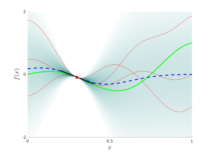
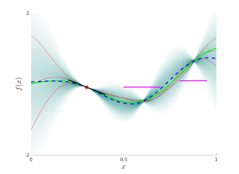
    

Refer to caption
(a) Posterior after one function observation and one derivative observation.
Refer to caption
(b) Posterior after one function observation, one derivative observation and two integral observations.
Figure 9: Example of GP regression with functional observations. The regression is done using one function observation (red circle), one derivative observation (tangential solid thick black line) and two integral observations (horizontal thick pink lines).

The procedure is easily extended to vector valued functions (Särkkä,, 2011). Letting 𝐱subscript𝐱\mathcal{L}_{\mathbf{\boldsymbol{\mathrm{x}}}} denote the transformation (such that an element in 𝐱subscript𝐱\mathcal{L}_{\mathbf{\boldsymbol{\mathrm{x}}}} is a linear operator), then we have that

𝐱𝐟𝒢𝒫(𝐱𝐦(𝐱),𝐱𝐊𝐟(𝐱,𝐱)𝐱𝖳).similar-tosubscript𝐱𝐟𝒢𝒫subscript𝐱𝐦𝐱subscript𝐱subscript𝐊𝐟𝐱superscript𝐱superscriptsubscriptsuperscript𝐱𝖳\mathcal{L}_{\mathbf{\boldsymbol{\mathrm{x}}}}\mathbf{\boldsymbol{\mathrm{f}}}\sim\mathcal{GP}(\mathcal{L}_{\mathbf{\boldsymbol{\mathrm{x}}}}\mathbf{\boldsymbol{\mathrm{m}}}(\mathbf{\boldsymbol{\mathrm{x}}}),\mathcal{L}_{\mathbf{\boldsymbol{\mathrm{x}}}}\mathbf{\boldsymbol{\mathrm{K}}}_{\mathbf{\boldsymbol{\mathrm{f}}}}(\mathbf{\boldsymbol{\mathrm{x}}},\mathbf{\boldsymbol{\mathrm{x}}}^{\prime})\mathcal{L}_{\mathbf{\boldsymbol{\mathrm{x}}}^{\prime}}^{\mathsf{T}}). (48)

Since the notation might suggest otherwise, we should emphasise that all operators in 𝐱𝐊(𝐱,𝐱)𝐱𝖳subscript𝐱𝐊𝐱superscript𝐱superscriptsubscriptsuperscript𝐱𝖳\mathcal{L}_{\mathbf{\boldsymbol{\mathrm{x}}}}\mathbf{\boldsymbol{\mathrm{K}}}(\mathbf{\boldsymbol{\mathrm{x}}},\mathbf{\boldsymbol{\mathrm{x}}}^{\prime})\mathcal{L}_{\mathbf{\boldsymbol{\mathrm{x}}}^{\prime}}^{\mathsf{T}} are applied to the elements in 𝐊𝐊\mathbf{\boldsymbol{\mathrm{K}}} from the right. As a simple example, assume that the function 𝐟(𝐱):22:𝐟𝐱maps-tosuperscript2superscript2\mathbf{\boldsymbol{\mathrm{f}}}(\mathbf{\boldsymbol{\mathrm{x}}}):\mathbb{R}^{2}\mapsto\mathbb{R}^{2} is modelled with a GP

𝐟(𝐱)𝐟𝐱\displaystyle\mathbf{\boldsymbol{\mathrm{f}}}(\mathbf{\boldsymbol{\mathrm{x}}}) 𝒢𝒫(𝟎,𝐊𝐟(𝐱,𝐱)),similar-toabsent𝒢𝒫0subscript𝐊𝐟𝐱superscript𝐱\displaystyle\sim\mathcal{GP}(\mathbf{\boldsymbol{\mathrm{0}}},\mathbf{\boldsymbol{\mathrm{K}}}_{\mathbf{\boldsymbol{\mathrm{f}}}}(\mathbf{\boldsymbol{\mathrm{x}}},\mathbf{\boldsymbol{\mathrm{x}}}^{\prime})), (49)
where
𝐊𝐟(𝐱,𝐱)subscript𝐊𝐟𝐱superscript𝐱\displaystyle\mathbf{\boldsymbol{\mathrm{K}}}_{\mathbf{\boldsymbol{\mathrm{f}}}}(\mathbf{\boldsymbol{\mathrm{x}}},\mathbf{\boldsymbol{\mathrm{x}}}^{\prime}) =[k11(𝐱,𝐱)k12(𝐱,𝐱)k21(𝐱,𝐱)k22(𝐱,𝐱)].absentmatrixsubscript𝑘11𝐱superscript𝐱subscript𝑘12𝐱superscript𝐱subscript𝑘21𝐱superscript𝐱subscript𝑘22𝐱superscript𝐱\displaystyle=\begin{bmatrix}k_{11}(\mathbf{\boldsymbol{\mathrm{x}}},\mathbf{\boldsymbol{\mathrm{x}}}^{\prime})&k_{12}(\mathbf{\boldsymbol{\mathrm{x}}},\mathbf{\boldsymbol{\mathrm{x}}}^{\prime})\\ k_{21}(\mathbf{\boldsymbol{\mathrm{x}}},\mathbf{\boldsymbol{\mathrm{x}}}^{\prime})&k_{22}(\mathbf{\boldsymbol{\mathrm{x}}},\mathbf{\boldsymbol{\mathrm{x}}}^{\prime})\end{bmatrix}. (50)

Assume further that

𝐠=[x00y]𝐟.𝐠matrix𝑥00𝑦𝐟\mathbf{\boldsymbol{\mathrm{g}}}=\begin{bmatrix}\frac{\partial}{\partial x}&0\\ 0&\frac{\partial}{\partial y}\end{bmatrix}\mathbf{\boldsymbol{\mathrm{f}}}. (51)

Now it follows from (48) that 𝐠𝐠\mathbf{\boldsymbol{\mathrm{g}}} is also a GP

𝐠(𝐱)𝐠𝐱\displaystyle\mathbf{\boldsymbol{\mathrm{g}}}(\mathbf{\boldsymbol{\mathrm{x}}}) 𝒢𝒫(𝐦𝐠,𝐊𝐠(𝐱,𝐱)),similar-toabsent𝒢𝒫subscript𝐦𝐠subscript𝐊𝐠𝐱superscript𝐱\displaystyle\sim\mathcal{GP}(\mathbf{\boldsymbol{\mathrm{m}}}_{\mathbf{\boldsymbol{\mathrm{g}}}},\mathbf{\boldsymbol{\mathrm{K}}}_{\mathbf{\boldsymbol{\mathrm{g}}}}(\mathbf{\boldsymbol{\mathrm{x}}},\mathbf{\boldsymbol{\mathrm{x}}}^{\prime})),
where
𝐦𝐠subscript𝐦𝐠\displaystyle\mathbf{\boldsymbol{\mathrm{m}}}_{\mathbf{\boldsymbol{\mathrm{g}}}} =[x00y]𝟎=𝟎,absentmatrix𝑥00𝑦00\displaystyle=\begin{bmatrix}\frac{\partial}{\partial x}&0\\ 0&\frac{\partial}{\partial y}\end{bmatrix}\mathbf{\boldsymbol{\mathrm{0}}}=\mathbf{\boldsymbol{\mathrm{0}}}, (52)

and

𝐊𝐠(𝐱,𝐱)subscript𝐊𝐠𝐱superscript𝐱\displaystyle\mathbf{\boldsymbol{\mathrm{K}}}_{\mathbf{\boldsymbol{\mathrm{g}}}}(\mathbf{\boldsymbol{\mathrm{x}}},\mathbf{\boldsymbol{\mathrm{x}}}^{\prime}) =[x00y][k11(𝐱,𝐱)k12(𝐱,𝐱)k21(𝐱,𝐱)k22(𝐱,𝐱)][x00y]𝖳=[2x2k11(𝐱,𝐱)2xyk12(𝐱,𝐱)2yxk21(𝐱,𝐱)2y2k22(𝐱,𝐱)].absentmatrix𝑥00𝑦matrixsubscript𝑘11𝐱superscript𝐱subscript𝑘12𝐱superscript𝐱subscript𝑘21𝐱superscript𝐱subscript𝑘22𝐱superscript𝐱superscriptmatrixsuperscript𝑥00superscript𝑦𝖳matrixsuperscript2superscript𝑥2subscript𝑘11𝐱superscript𝐱superscript2𝑥superscript𝑦subscript𝑘12𝐱superscript𝐱superscript2𝑦superscript𝑥subscript𝑘21𝐱superscript𝐱superscript2superscript𝑦2subscript𝑘22𝐱superscript𝐱\displaystyle=\begin{bmatrix}\frac{\partial}{\partial x}&0\\ 0&\frac{\partial}{\partial y}\end{bmatrix}\begin{bmatrix}k_{11}(\mathbf{\boldsymbol{\mathrm{x}}},\mathbf{\boldsymbol{\mathrm{x}}}^{\prime})&k_{12}(\mathbf{\boldsymbol{\mathrm{x}}},\mathbf{\boldsymbol{\mathrm{x}}}^{\prime})\\ k_{21}(\mathbf{\boldsymbol{\mathrm{x}}},\mathbf{\boldsymbol{\mathrm{x}}}^{\prime})&k_{22}(\mathbf{\boldsymbol{\mathrm{x}}},\mathbf{\boldsymbol{\mathrm{x}}}^{\prime})\end{bmatrix}\begin{bmatrix}\frac{\partial}{\partial x^{\prime}}&0\\ 0&\frac{\partial}{\partial y^{\prime}}\end{bmatrix}^{\mathsf{T}}=\begin{bmatrix}\frac{\partial^{2}}{\partial x^{2}}k_{11}(\mathbf{\boldsymbol{\mathrm{x}}},\mathbf{\boldsymbol{\mathrm{x}}}^{\prime})&\frac{\partial^{2}}{\partial x\partial y^{\prime}}k_{12}(\mathbf{\boldsymbol{\mathrm{x}}},\mathbf{\boldsymbol{\mathrm{x}}}^{\prime})\\[2.84526pt] \frac{\partial^{2}}{\partial y\partial x^{\prime}}k_{21}(\mathbf{\boldsymbol{\mathrm{x}}},\mathbf{\boldsymbol{\mathrm{x}}}^{\prime})&\frac{\partial^{2}}{\partial y^{2}}k_{22}(\mathbf{\boldsymbol{\mathrm{x}}},\mathbf{\boldsymbol{\mathrm{x}}}^{\prime})\end{bmatrix}. (53)

Using a covariance function with this particular structure ensures that the relation (51) is fulfilled.

Appendix C Building the covariance function using the Airy stress function

To ensure a physical solution, our model should obey the essential equilibrium constraints, which must be fulfilled by the strain field at all points. As described by Sadd, (2005, p. 132), the equilibrium constraints for a two dimensional stress field are given by

σ~xxx+σxyy=0,subscript~𝜎𝑥𝑥𝑥subscript𝜎𝑥𝑦𝑦0\displaystyle\frac{\partial\tilde{\sigma}_{xx}}{\partial x}+\frac{\partial\sigma_{xy}}{\partial y}=0, (54a)
σxyx+σ~yyy=0,subscript𝜎𝑥𝑦𝑥subscript~𝜎𝑦𝑦𝑦0\displaystyle\frac{\partial\sigma_{xy}}{\partial x}+\frac{\partial\tilde{\sigma}_{yy}}{\partial y}=0, (54b)

where σ~xx=σxxVsubscript~𝜎𝑥𝑥subscript𝜎𝑥𝑥𝑉\tilde{\sigma}_{xx}=\sigma_{xx}-V, σ~yy=σyyVsubscript~𝜎𝑦𝑦subscript𝜎𝑦𝑦𝑉\tilde{\sigma}_{yy}=\sigma_{yy}-V and V𝑉V is a potential function. These equations are satisfied by letting the components be represented as

σ~xxsubscript~𝜎𝑥𝑥\displaystyle\tilde{\sigma}_{xx} =2φy2,absentsuperscript2𝜑superscript𝑦2\displaystyle=\frac{\partial^{2}\varphi}{\partial y^{2}}, (55a)
σxysubscript𝜎𝑥𝑦\displaystyle\sigma_{xy} =2φxy,absentsuperscript2𝜑𝑥𝑦\displaystyle=-\frac{\partial^{2}\varphi}{\partial x\partial y}, (55b)
σ~yysubscript~𝜎𝑦𝑦\displaystyle\tilde{\sigma}_{yy} =2φx2,absentsuperscript2𝜑superscript𝑥2\displaystyle=\frac{\partial^{2}\varphi}{\partial x^{2}}, (55c)

where the arbitrary scalar function φ=φ(x,y)𝜑𝜑𝑥𝑦\varphi=\varphi(x,y) is the so-called Airy stress function. Letting V=0𝑉0V=0 to keep the notation uncluttered, we have that

[σxxσxyσyy]=[2y22xy2x2]φ.matrixsubscript𝜎𝑥𝑥subscript𝜎𝑥𝑦subscript𝜎𝑦𝑦matrixsuperscript2superscript𝑦2superscript2𝑥𝑦superscript2superscript𝑥2𝜑\begin{bmatrix}\sigma_{xx}\\ \sigma_{xy}\\ \sigma_{yy}\end{bmatrix}=\begin{bmatrix}\frac{\partial^{2}}{\partial y^{2}}\\[2.84526pt] -\frac{\partial^{2}}{\partial x\partial y}\\[2.84526pt] \frac{\partial^{2}}{\partial x^{2}}\end{bmatrix}\varphi. (56)

Applying Hooke’s law for isotropic linearly elastic solid materials

[ϵxxϵxyϵyy]=1E[10ν01+ν0ν01][σxxσxyσyy],matrixsubscriptitalic-ϵ𝑥𝑥subscriptitalic-ϵ𝑥𝑦subscriptitalic-ϵ𝑦𝑦1𝐸matrix10𝜈01𝜈0𝜈01matrixsubscript𝜎𝑥𝑥subscript𝜎𝑥𝑦subscript𝜎𝑦𝑦\begin{bmatrix}\epsilon_{xx}\\ \epsilon_{xy}\\ \epsilon_{yy}\end{bmatrix}=\frac{1}{E}\begin{bmatrix}1&0&-\nu\\ 0&1+\nu&0\\ -\nu&0&1\end{bmatrix}\begin{bmatrix}\sigma_{xx}\\ \sigma_{xy}\\ \sigma_{yy}\end{bmatrix}, (57)

where E𝐸E and ν𝜈\nu denote Young’s modulus and Poisson’s ratio, respectively, we end up with

𝐟=[ϵxxϵxyϵyy]=1E[10ν01+ν0ν01][2y22xy2x2]φ=1E[2y2ν2x2(1+ν)2xy2x2ν2y2]φ=𝐱φ.𝐟matrixsubscriptitalic-ϵ𝑥𝑥subscriptitalic-ϵ𝑥𝑦subscriptitalic-ϵ𝑦𝑦1𝐸matrix10𝜈01𝜈0𝜈01matrixsuperscript2superscript𝑦2superscript2𝑥𝑦superscript2superscript𝑥2𝜑1𝐸matrixsuperscript2superscript𝑦2𝜈superscript2superscript𝑥21𝜈superscript2𝑥𝑦superscript2superscript𝑥2𝜈superscript2superscript𝑦2𝜑subscript𝐱𝜑\displaystyle\mathbf{\boldsymbol{\mathrm{f}}}=\begin{bmatrix}\epsilon_{xx}\\ \epsilon_{xy}\\ \epsilon_{yy}\end{bmatrix}=\frac{1}{E}\begin{bmatrix}1&0&-\nu\\ 0&1+\nu&0\\ -\nu&0&1\end{bmatrix}\begin{bmatrix}\frac{\partial^{2}}{\partial y^{2}}\\[2.84526pt] -\frac{\partial^{2}}{\partial x\partial y}\\[2.84526pt] \frac{\partial^{2}}{\partial x^{2}}\end{bmatrix}\varphi=\frac{1}{E}\begin{bmatrix}\frac{\partial^{2}}{\partial y^{2}}-\nu\frac{\partial^{2}}{\partial x^{2}}\\[2.84526pt] (1+\nu)\frac{\partial^{2}}{\partial x\partial y}\\[2.84526pt] \frac{\partial^{2}}{\partial x^{2}}-\nu\frac{\partial^{2}}{\partial y^{2}}\end{bmatrix}\varphi=\mathcal{L}_{\mathbf{\boldsymbol{\mathrm{x}}}}\varphi. (58)

Let us now model φ𝜑\varphi as a GP

φ𝒢𝒫(0,kφ(𝐱,𝐱)).similar-to𝜑𝒢𝒫0subscript𝑘𝜑𝐱superscript𝐱\varphi\sim\mathcal{GP}(0,k_{\varphi}(\mathbf{\boldsymbol{\mathrm{x}}},\mathbf{\boldsymbol{\mathrm{x}}}^{\prime})). (59)

Since the strain field 𝐟𝐟\mathbf{\boldsymbol{\mathrm{f}}} is mapped from φ𝜑\varphi through the linear functional 𝐱subscript𝐱\mathcal{L}_{\mathbf{\boldsymbol{\mathrm{x}}}}, it follows from Section B that it is also a GP

𝐟𝒢𝒫(𝟎,𝐱kφ(𝐱,𝐱)𝐱𝖳).similar-to𝐟𝒢𝒫0subscript𝐱subscript𝑘𝜑𝐱superscript𝐱superscriptsubscriptsuperscript𝐱𝖳\mathbf{\boldsymbol{\mathrm{f}}}\sim\mathcal{GP}(\boldsymbol{0},\mathcal{L}_{\mathbf{\boldsymbol{\mathrm{x}}}}k_{\varphi}(\mathbf{\boldsymbol{\mathrm{x}}},\mathbf{\boldsymbol{\mathrm{x}}}^{\prime})\mathcal{L}_{\mathbf{\boldsymbol{\mathrm{x}}}^{\prime}}^{\mathsf{T}}). (60)

Building the covariance function this way will by construction guarantee that any sample drawn from the resulting posterior fulfils the equilibrium constraints given by (54).

Appendix D Details on approximative computations

D.1 Elements of the 𝐐𝐐\mathbf{\boldsymbol{\mathrm{Q}}}-matrix

As stated in (8), the target function 𝐟(𝐱)𝐟𝐱\mathbf{\boldsymbol{\mathrm{f}}}(\mathbf{\boldsymbol{\mathrm{x}}}) is related to the scalar function φ(x,y)𝜑𝑥𝑦\varphi(x,y) according to

𝐟(𝐱)=[2y2ν2x2(1+ν)2xy2x2ν2y2]φ(x,y)=𝐱φ(x,y).𝐟𝐱matrixsuperscript2superscript𝑦2𝜈superscript2superscript𝑥21𝜈superscript2𝑥𝑦superscript2superscript𝑥2𝜈superscript2superscript𝑦2𝜑𝑥𝑦subscript𝐱𝜑𝑥𝑦\begin{split}\mathbf{\boldsymbol{\mathrm{f}}}(\mathbf{\boldsymbol{\mathrm{x}}})=\begin{bmatrix}\frac{\partial^{2}}{\partial y^{2}}-\nu\frac{\partial^{2}}{\partial x^{2}}\\[2.84526pt] (1+\nu)\frac{\partial^{2}}{\partial x\partial y}\\[2.84526pt] \frac{\partial^{2}}{\partial x^{2}}-\nu\frac{\partial^{2}}{\partial y^{2}}\end{bmatrix}\varphi(x,y)=\mathcal{L}_{\mathbf{\boldsymbol{\mathrm{x}}}}\varphi(x,y).\end{split} (61)

In the approximative method described in Section 4.1, we are projecting the functional (16) onto the basis functions

ϕ(𝐱)italic-ϕ𝐱\displaystyle\phi(\mathbf{\boldsymbol{\mathrm{x}}}) =1ρxρysin(λx(x+ρx))sin(λy(y+ρy)).absent1subscript𝜌𝑥subscript𝜌𝑦subscript𝜆𝑥𝑥subscript𝜌𝑥subscript𝜆𝑦𝑦subscript𝜌𝑦\displaystyle=\frac{1}{\sqrt{\rho_{x}\rho_{y}}}\sin\big{(}\lambda_{x}(x+\rho_{x})\big{)}\sin\big{(}\lambda_{y}(y+\rho_{y})\big{)}. (62)

To keep the notation uncluttered, we are in this section omitting the indexing of the basis functions as well as the measurements, but keep in mind that each calculation described by the equations below must be repeated m𝑚m times for each measurement.

Each measurement with inputs 𝐱0superscript𝐱0\mathbf{\boldsymbol{\mathrm{x}}}^{0}, L𝐿L and 𝐧^^𝐧\hat{\mathbf{n}} requires us to calculate the integral

1L0Larg(x0+snx,y0+sny)𝑑s,1𝐿superscriptsubscript0𝐿argsuperscript𝑥0𝑠subscript𝑛𝑥superscript𝑦0𝑠subscript𝑛𝑦differential-d𝑠\frac{1}{L}\int_{0}^{L}\text{arg}(x^{0}+sn_{x},y^{0}+sn_{y})ds, (63)

where

arg(x,y)=𝐧𝖳𝐱ϕ(x,y)=[nx2(2y2ν2x2)+2nxny(1+ν)2xy+ny2(2x2ν2y2)]ϕ(x,y).arg𝑥𝑦superscript𝐧𝖳subscript𝐱italic-ϕ𝑥𝑦delimited-[]superscriptsubscript𝑛𝑥2superscript2superscript𝑦2𝜈superscript2superscript𝑥22subscript𝑛𝑥subscript𝑛𝑦1𝜈superscript2𝑥𝑦superscriptsubscript𝑛𝑦2superscript2superscript𝑥2𝜈superscript2superscript𝑦2italic-ϕ𝑥𝑦\displaystyle\text{arg}(x,y)=\vec{\mathbf{\boldsymbol{\mathrm{n}}}}^{\mathsf{T}}\mathcal{L}_{\mathbf{\boldsymbol{\mathrm{x}}}}\phi(x,y)=\bigg{[}n_{x}^{2}\left(\frac{\partial^{2}}{\partial y^{2}}-\nu\frac{\partial^{2}}{\partial x^{2}}\right)+2n_{x}n_{y}(1+\nu)\frac{\partial^{2}}{\partial x\partial y}+n_{y}^{2}\left(\frac{\partial^{2}}{\partial x^{2}}-\nu\frac{\partial^{2}}{\partial y^{2}}\right)\bigg{]}\phi(x,y). (64)

The partial derivatives involved have the following explicit forms

2x2superscript2superscript𝑥2\displaystyle\frac{\partial^{2}}{\partial x^{2}} ϕ(x,y)=λx2ϕ(x,y),italic-ϕ𝑥𝑦superscriptsubscript𝜆𝑥2italic-ϕ𝑥𝑦\displaystyle\phi(x,y)=-\lambda_{x}^{2}\phi(x,y), (65a)
2xysuperscript2𝑥𝑦\displaystyle\frac{\partial^{2}}{\partial x\partial y} ϕ(x,y)=λxλy1ρxρycos(λx(x+ρx))cos(λy(y+ρy))ϕc(x,y),italic-ϕ𝑥𝑦subscript𝜆𝑥subscript𝜆𝑦subscript1subscript𝜌𝑥subscript𝜌𝑦subscript𝜆𝑥𝑥subscript𝜌𝑥subscript𝜆𝑦𝑦subscript𝜌𝑦subscriptitalic-ϕ𝑐𝑥𝑦\displaystyle\phi(x,y)=\lambda_{x}\lambda_{y}\underbrace{\frac{1}{\sqrt{\rho_{x}\rho_{y}}}\cos\big{(}\lambda_{x}(x+\rho_{x})\big{)}\cos\big{(}\lambda_{y}(y+\rho_{y})\big{)}}_{\phi_{c}(x,y)}, (65b)
2y2superscript2superscript𝑦2\displaystyle\frac{\partial^{2}}{\partial y^{2}} ϕ(x,y)=λy2ϕ(x,y).italic-ϕ𝑥𝑦superscriptsubscript𝜆𝑦2italic-ϕ𝑥𝑦\displaystyle\phi(x,y)=-\lambda_{y}^{2}\phi(x,y). (65c)

Substituting the expressions (65) into (64) yields

arg(x,y)=[nx2(νλx2λy2)+ny2(νλy2λx2)]CSϕ(x,y)+2(1+ν)nxnyλxλyCOϕC(x,y).arg𝑥𝑦subscriptdelimited-[]superscriptsubscript𝑛𝑥2𝜈superscriptsubscript𝜆𝑥2superscriptsubscript𝜆𝑦2superscriptsubscript𝑛𝑦2𝜈superscriptsubscript𝜆𝑦2superscriptsubscript𝜆𝑥2subscript𝐶𝑆italic-ϕ𝑥𝑦subscript21𝜈subscript𝑛𝑥subscript𝑛𝑦subscript𝜆𝑥subscript𝜆𝑦subscript𝐶𝑂subscriptitalic-ϕ𝐶𝑥𝑦\displaystyle\text{arg}(x,y)=\underbrace{\left[n_{x}^{2}\left(\nu\lambda_{x}^{2}-\lambda_{y}^{2}\right)+n_{y}^{2}\left(\nu\lambda_{y}^{2}-\lambda_{x}^{2}\right)\right]}_{C_{S}}\phi(x,y)+\underbrace{2(1+\nu)n_{x}n_{y}\lambda_{x}\lambda_{y}}_{C_{O}}\phi_{C}(x,y). (66)

We can now see that (63) involves calculation of the two integrals

I1=0Lϕ(x+snx,y+sny)𝑑s=12ρxρy[1Λsin(Λs+B)1Λ+sin(Λ+s+B+)]s=0s=L,subscript𝐼1superscriptsubscript0𝐿italic-ϕ𝑥𝑠subscript𝑛𝑥𝑦𝑠subscript𝑛𝑦differential-d𝑠12subscript𝜌𝑥subscript𝜌𝑦superscriptsubscriptdelimited-[]1superscriptΛsuperscriptΛ𝑠superscript𝐵1superscriptΛsuperscriptΛ𝑠superscript𝐵𝑠0𝑠𝐿\displaystyle I_{1}=\int_{0}^{L}\phi(x+sn_{x},y+sn_{y})ds=\frac{1}{2\sqrt{\rho_{x}\rho_{y}}}\bigg{[}\frac{1}{\Lambda^{-}}\sin(\Lambda^{-}s+B^{-})-\frac{1}{\Lambda^{+}}\sin(\Lambda^{+}s+B^{+})\bigg{]}_{s=0}^{s=L}, (67a)
I2=0LϕC(x+snx,y+sny)𝑑s=12ρxρy[1Λsin(Λs+B)+1Λ+sin(Λ+s+B+)]s=0s=L,subscript𝐼2superscriptsubscript0𝐿subscriptitalic-ϕ𝐶𝑥𝑠subscript𝑛𝑥𝑦𝑠subscript𝑛𝑦differential-d𝑠12subscript𝜌𝑥subscript𝜌𝑦superscriptsubscriptdelimited-[]1superscriptΛsuperscriptΛ𝑠superscript𝐵1superscriptΛsuperscriptΛ𝑠superscript𝐵𝑠0𝑠𝐿\displaystyle I_{2}=\int_{0}^{L}\phi_{C}(x+sn_{x},y+sn_{y})ds=\frac{1}{2\sqrt{\rho_{x}\rho_{y}}}\bigg{[}\frac{1}{\Lambda^{-}}\sin(\Lambda^{-}s+B^{-})+\frac{1}{\Lambda^{+}}\sin(\Lambda^{+}s+B^{+})\bigg{]}_{s=0}^{s=L}, (67b)

where we have defined

Λ±superscriptΛplus-or-minus\displaystyle\Lambda^{\pm} =nxλx±nyλy,absentplus-or-minussubscript𝑛𝑥subscript𝜆𝑥subscript𝑛𝑦subscript𝜆𝑦\displaystyle=n_{x}\lambda_{x}\pm n_{y}\lambda_{y}, (68a)
B±superscript𝐵plus-or-minus\displaystyle B^{\pm} =λx(x0+ρx)±λy(y0+ρy).absentplus-or-minussubscript𝜆𝑥superscript𝑥0subscript𝜌𝑥subscript𝜆𝑦superscript𝑦0subscript𝜌𝑦\displaystyle=\lambda_{x}(x^{0}+\rho_{x})\pm\lambda_{y}(y^{0}+\rho_{y}). (68b)

Finally, we end up with

1L0Larg(x0+snx,y0+sny)𝑑s=CSI1+COI2L.1𝐿superscriptsubscript0𝐿argsuperscript𝑥0𝑠subscript𝑛𝑥superscript𝑦0𝑠subscript𝑛𝑦differential-d𝑠subscript𝐶𝑆subscript𝐼1subscript𝐶𝑂subscript𝐼2𝐿\frac{1}{L}\int_{0}^{L}\text{arg}(x^{0}+sn_{x},y^{0}+sn_{y})ds=\frac{C_{S}I_{1}+C_{O}I_{2}}{L}. (69)

Hence, the element 𝐐ijsubscript𝐐𝑖𝑗\mathbf{\boldsymbol{\mathrm{Q}}}_{ij} in (29) is obtained by in the above calculations use the i𝑖i:th basis function with corresponding eigenvalues, and the input arguments of the j𝑗j:th measurement.

D.2 Marginal Likelihood Expressions

By replacing 𝐊Isubscript𝐊I\mathbf{\boldsymbol{\mathrm{K}}}_{\mathrm{I}} in (31) with the approximation 𝐊I𝐐𝖳𝚲𝐐,subscript𝐊Isuperscript𝐐𝖳𝚲𝐐\mathbf{\boldsymbol{\mathrm{K}}}_{\mathrm{I}}\approx\mathbf{\boldsymbol{\mathrm{Q}}}^{\mathsf{T}}\boldsymbol{\Lambda}\mathbf{\boldsymbol{\mathrm{Q}}}, and letting 𝐐^=𝐐𝖳𝚲𝐐+σ2I^𝐐superscript𝐐𝖳𝚲𝐐superscript𝜎2𝐼\hat{\mathbf{\mathbf{\boldsymbol{\mathrm{Q}}}}}=\mathbf{\boldsymbol{\mathrm{Q}}}^{\mathsf{T}}\boldsymbol{\Lambda}\mathbf{\boldsymbol{\mathrm{Q}}}+\sigma^{2}I, we get the following expression for the logarithm of the approximate marginal likelihood

logp(𝐲|{𝜼i},𝜽)logp~(𝐲|{𝜼i},𝜽)=12logdet(𝐐^)12𝐲𝖳𝐐^1𝐲N2log2π.𝑝conditional𝐲subscript𝜼𝑖𝜽~𝑝conditional𝐲subscript𝜼𝑖𝜽12^𝐐12superscript𝐲𝖳superscript^𝐐1𝐲𝑁22𝜋\displaystyle\log p(\mathbf{\boldsymbol{\mathrm{y}}}|\{\boldsymbol{\eta}_{i}\},\boldsymbol{\theta})\approx\log\tilde{p}(\mathbf{\boldsymbol{\mathrm{y}}}|\{\boldsymbol{\eta}_{i}\},\boldsymbol{\theta})=-\frac{1}{2}\log\det(\hat{\mathbf{\mathbf{\boldsymbol{\mathrm{Q}}}}})-\frac{1}{2}\mathbf{\boldsymbol{\mathrm{y}}}^{\mathsf{T}}\hat{\mathbf{\mathbf{\boldsymbol{\mathrm{Q}}}}}^{-1}\mathbf{\boldsymbol{\mathrm{y}}}-\frac{N}{2}\log 2\pi. (70)

For simplicity, we separate the partial derivative with respect to the noise σ𝜎\sigma and the partial derivatives with respect to the other hyperparameters:

θilogp~(𝐲|{𝜼i},𝜽)=12logdet(𝐐^)θi12𝐲𝖳𝐐^1𝐲θi,subscript𝜃𝑖~𝑝conditional𝐲subscript𝜼𝑖𝜽12^𝐐subscript𝜃𝑖12superscript𝐲𝖳superscript^𝐐1𝐲subscript𝜃𝑖\displaystyle\frac{\partial}{\partial\theta_{i}}\log\tilde{p}(\mathbf{\boldsymbol{\mathrm{y}}}|\{\boldsymbol{\eta}_{i}\},\boldsymbol{\theta})=-\frac{1}{2}\frac{\partial\log\det(\hat{\mathbf{\mathbf{\boldsymbol{\mathrm{Q}}}}})}{\partial\theta_{i}}-\frac{1}{2}\frac{\partial\mathbf{\boldsymbol{\mathrm{y}}}^{\mathsf{T}}\hat{\mathbf{\mathbf{\boldsymbol{\mathrm{Q}}}}}^{-1}\mathbf{\boldsymbol{\mathrm{y}}}}{\partial\theta_{i}}, (71a)
σlogp~(𝐲|{𝜼i},𝜽)=12logdet(𝐐^)σ12𝐲𝖳𝐐^1𝐲σ.𝜎~𝑝conditional𝐲subscript𝜼𝑖𝜽12^𝐐𝜎12superscript𝐲𝖳superscript^𝐐1𝐲𝜎\displaystyle\frac{\partial}{\partial\sigma}\log\tilde{p}(\mathbf{\boldsymbol{\mathrm{y}}}|\{\boldsymbol{\eta}_{i}\},\boldsymbol{\theta})=-\frac{1}{2}\frac{\partial\log\det(\hat{\mathbf{\mathbf{\boldsymbol{\mathrm{Q}}}}})}{\partial\sigma}-\frac{1}{2}\frac{\partial\mathbf{\boldsymbol{\mathrm{y}}}^{\mathsf{T}}\hat{\mathbf{\mathbf{\boldsymbol{\mathrm{Q}}}}}^{-1}\mathbf{\boldsymbol{\mathrm{y}}}}{\partial\sigma}. (71b)

Introducing 𝐙=σ2𝚲1+𝐐𝐐𝖳𝐙superscript𝜎2superscript𝚲1superscript𝐐𝐐𝖳\mathbf{\boldsymbol{\mathrm{Z}}}=\sigma^{2}\boldsymbol{\Lambda}^{-1}+\mathbf{\boldsymbol{\mathrm{Q}}}\mathbf{\boldsymbol{\mathrm{Q}}}^{\mathsf{T}}, the explicit expressions are:

logdet(𝐐^)^𝐐\displaystyle\log\det(\hat{\mathbf{\mathbf{\boldsymbol{\mathrm{Q}}}}}) =(Nm)logσ2logdet(𝐙)jlog𝚲jj,absent𝑁𝑚superscript𝜎2𝐙subscript𝑗subscript𝚲𝑗𝑗\displaystyle=-(N-m)\log\sigma^{2}-\log\det(\mathbf{\boldsymbol{\mathrm{Z}}})-\sum_{j}\log\boldsymbol{\Lambda}_{jj}, (72a)
logdet(𝐐^)θi^𝐐subscript𝜃𝑖\displaystyle\frac{\partial\log\det(\hat{\mathbf{\mathbf{\boldsymbol{\mathrm{Q}}}}})}{\partial\theta_{i}} =j𝚲jj𝚲jjθi+σ2tr(𝐙1𝚲2𝚲θi),absentsubscript𝑗subscript𝚲𝑗𝑗subscript𝚲𝑗𝑗subscript𝜃𝑖superscript𝜎2trsuperscript𝐙1superscript𝚲2𝚲subscript𝜃𝑖\displaystyle=-\sum_{j}\boldsymbol{\Lambda}_{jj}\frac{\partial\boldsymbol{\Lambda}_{jj}}{\partial\theta_{i}}+\sigma^{2}\text{tr}\left(\mathbf{\boldsymbol{\mathrm{Z}}}^{-1}\boldsymbol{\Lambda}^{-2}\frac{\partial\boldsymbol{\Lambda}}{\partial\theta_{i}}\right), (72b)
logdet(𝐐^)σ^𝐐𝜎\displaystyle\frac{\partial\log\det(\hat{\mathbf{\mathbf{\boldsymbol{\mathrm{Q}}}}})}{\partial\sigma} =2Nmσ2σtr(𝐙1𝚲1),absent2𝑁𝑚𝜎2𝜎trsuperscript𝐙1superscript𝚲1\displaystyle=-2\frac{N-m}{\sigma}-2\sigma\text{tr}\left(\mathbf{\boldsymbol{\mathrm{Z}}}^{-1}\boldsymbol{\Lambda}^{-1}\right), (72c)
12𝐲𝖳𝐐^1𝐲12superscript𝐲𝖳superscript^𝐐1𝐲\displaystyle\frac{1}{2}\mathbf{\boldsymbol{\mathrm{y}}}^{\mathsf{T}}\hat{\mathbf{\mathbf{\boldsymbol{\mathrm{Q}}}}}^{-1}\mathbf{\boldsymbol{\mathrm{y}}} =1σ2(𝐲𝖳𝐐𝖳𝐙1𝐐𝐲),absent1superscript𝜎2superscript𝐲𝖳superscript𝐐𝖳superscript𝐙1𝐐𝐲\displaystyle=\frac{1}{\sigma^{2}}\left(\mathbf{\boldsymbol{\mathrm{y}}}^{\mathsf{T}}\mathbf{\boldsymbol{\mathrm{Q}}}^{\mathsf{T}}\mathbf{\boldsymbol{\mathrm{Z}}}^{-1}\mathbf{\boldsymbol{\mathrm{Q}}}\mathbf{\boldsymbol{\mathrm{y}}}\right), (72d)
𝐲𝖳𝐐^1𝐲θisuperscript𝐲𝖳superscript^𝐐1𝐲subscript𝜃𝑖\displaystyle\frac{\partial\mathbf{\boldsymbol{\mathrm{y}}}^{\mathsf{T}}\hat{\mathbf{\mathbf{\boldsymbol{\mathrm{Q}}}}}^{-1}\mathbf{\boldsymbol{\mathrm{y}}}}{\partial\theta_{i}} =𝐲𝖳𝐐𝖳𝐙1[𝚲2𝚲θi]𝐙1𝐐𝐲,absentsuperscript𝐲𝖳superscript𝐐𝖳superscript𝐙1delimited-[]superscript𝚲2𝚲subscript𝜃𝑖superscript𝐙1𝐐𝐲\displaystyle=\mathbf{\boldsymbol{\mathrm{y}}}^{\mathsf{T}}\mathbf{\boldsymbol{\mathrm{Q}}}^{\mathsf{T}}\mathbf{\boldsymbol{\mathrm{Z}}}^{-1}\left[\boldsymbol{\Lambda}^{-2}\frac{\partial\boldsymbol{\Lambda}}{\partial\theta_{i}}\right]\mathbf{\boldsymbol{\mathrm{Z}}}^{-1}\mathbf{\boldsymbol{\mathrm{Q}}}\mathbf{\boldsymbol{\mathrm{y}}}, (72e)
𝐲𝖳𝐐^1𝐲σsuperscript𝐲𝖳superscript^𝐐1𝐲𝜎\displaystyle\frac{\partial\mathbf{\boldsymbol{\mathrm{y}}}^{\mathsf{T}}\hat{\mathbf{\mathbf{\boldsymbol{\mathrm{Q}}}}}^{-1}\mathbf{\boldsymbol{\mathrm{y}}}}{\partial\sigma} =2σ𝐲𝖳𝐐𝖳𝐙1𝚲1𝐙1𝐐𝐲+2σ3𝐲𝖳𝐲2σ3𝐲𝖳𝐐𝖳𝐙1𝐐𝐲.absent2𝜎superscript𝐲𝖳superscript𝐐𝖳superscript𝐙1superscript𝚲1superscript𝐙1𝐐𝐲2superscript𝜎3superscript𝐲𝖳𝐲2superscript𝜎3superscript𝐲𝖳superscript𝐐𝖳superscript𝐙1𝐐𝐲\displaystyle=-\frac{2}{\sigma}\mathbf{\boldsymbol{\mathrm{y}}}^{\mathsf{T}}\mathbf{\boldsymbol{\mathrm{Q}}}^{\mathsf{T}}\mathbf{\boldsymbol{\mathrm{Z}}}^{-1}\boldsymbol{\Lambda}^{-1}\mathbf{\boldsymbol{\mathrm{Z}}}^{-1}\mathbf{\boldsymbol{\mathrm{Q}}}\mathbf{\boldsymbol{\mathrm{y}}}+\frac{2}{\sigma^{3}}\mathbf{\boldsymbol{\mathrm{y}}}^{\mathsf{T}}\mathbf{\boldsymbol{\mathrm{y}}}-\frac{2}{\sigma^{3}}\mathbf{\boldsymbol{\mathrm{y}}}^{\mathsf{T}}\mathbf{\boldsymbol{\mathrm{Q}}}^{\mathsf{T}}\mathbf{\boldsymbol{\mathrm{Z}}}^{-1}\mathbf{\boldsymbol{\mathrm{Q}}}\mathbf{\boldsymbol{\mathrm{y}}}. (72f)

References

  • Calandra et al., (2016) Calandra, R., Peters, J., Rasmussen, C. E., and Deisenroth, M. P. (2016). Manifold Gaussian processes for regression. In In Proceedings of the International Joint Conference on Neural Networks, pages 3338–3345.
  • Damianou, (2015) Damianou, A. (2015). Deep Gaussian processes and variational propagation of uncertainty. PhD thesis, Department of neuroscience, University of Sheffield.
  • Fitzpatrick and Lodini, (2003) Fitzpatrick, M. and Lodini, A. (2003). Analysis of Residual Stress by Diffraction Using Neutron and Synchrotron Radiation. CRC Press.
  • Garnett, (2017) Garnett, R. (2017). Lecture 11: Bayesian quadrature. University Lecture. Accessed: 2017-05-05. Available from: http://www.cse.wustl.edu/~garnett/cse515t/spring_2017/files/lecture_notes/11.pdf.
  • Ghahramani, (2015) Ghahramani, Z. (2015). Probabilistic machine learning and artificial intelligence. Nature, 521:452–459.
  • Hendriks et al., (2017) Hendriks, J. N., Gregg, A. W. T., Wensrich, C. M., Tremsin, A. S., Shinohara, T., Meylan, M., Kisi, E. H., Luzin, V., and Kirsten, O. (2017). Bragg-edge elastic strain tomography for in situ systems from energy-resolved neutron transmission imaging. Physical Review Materials, 1(5):053802.
  • Hennig and Kiefel, (2013) Hennig, P. and Kiefel, M. (2013). Quasi-Newton methods: A new direction. The Journal of Machine Learning Research, 14(1):843–865.
  • Jidling et al., (2017) Jidling, C., Wahlström, N., Wills, A., and Schön, T. B. (2017). Linearly constrained gaussian processes. In Advances in Neural Information Processing Systems 30, pages 1215–1224. Curran Associates, Inc.
  • Korsunsky et al., (2011) Korsunsky, A. M., Baimpas, N., Song, X., Belnoue, J., Hofmann, F., Abbey, B., Xie, M., Andrieux, J., Buslaps, T., and Neo, T. K. (2011). Strain tomography of polycrystalline zirconia dental prostheses by synchrotron x-ray diffraction. Acta Materialia, 59(6):2501–2513.
  • Korsunsky et al., (2008) Korsunsky, A. M., Vorster, W. J., Zhang, S. Y., Dini, D., Latham, D., Golshan, M., Liu, J., Kyriakoglou, Y., and Walsh, M. J. (2008). The principle of strain reconstruction tomography: Determination of quench strain distribution from diffraction measurements. Acta Materiala, 54(8):2101–2108.
  • Lionheart and Withers, (2015) Lionheart, W. R. B. and Withers, P. J. (2015). Diffraction tomography of strain. Inverse Problems, 31(4):045005.
  • Nocedal and Wright, (2000) Nocedal, J. and Wright, S. (2000). Numerical Optimization. Springer Series in Operations Research and Financial Engineering. Springer New York.
  • Noyan and Cohen, (2013) Noyan, I. and Cohen, J. (2013). Residual stress: measurement by diffraction and interpretation. Springer.
  • Papoulis and Pillai, (1991) Papoulis, A. and Pillai, S. U. (1991). Probability, random variables, and stochastic processes. McGraw-Hill Education, New York.
  • Prime, (2001) Prime, M. B. (2001). Cross-sectional mapping of residual stresses by measuring the surface contour after a cut. Transactions-American society of mechanical engineers journal of engineering materials and technology, 123(2):162–168.
  • Quiñonero Candela et al., (2007) Quiñonero Candela, J., Ramussen, C. E., and Williams, C. K. I. (2007). Approximation methods for gaussian process regression. Large-scale kernel machines, pages 203–223.
  • Rasmussen and Williams, (2006) Rasmussen, C. E. and Williams, C. K. I. (2006). Gaussian processes for machine learning. MIT press, Cambridge, MA.
  • Sadd, (2005) Sadd, M. H. (2005). Elasticity - Theory, applications and numerics. New York: Elsevier Butterworth-Heinemann.
  • (19) Santisteban, J., Edwards, L., Fitzpatrick, M., Steuwer, A., Withers, P., Daymond, M., Johnson, M., Rhodes, N., and Schooneveld, E. (2002a). Strain imaging by bragg edge neutron transmission. Nuclear Instruments and Methods in Physics Research Section A: Accelerators, Spectrometers, Detectors and Associated Equipment, 481(1):765–768.
  • (20) Santisteban, J., Edwards, L., Fizpatrick, M., Steuwer, A., and Withers, P. (2002b). Engineering applications of Bragg-edge neutron transmission. Applied Physics, 74(1):1433–1436.
  • Särkkä, (2011) Särkkä, S. (2011). Linear operators and stochastic partial differential equations in Gaussian process regression. In Proceedings of the Artificial Neural Networks and Machine Learning – ICANN 2011, pages 151–158. Springer.
  • Sato et al., (2011) Sato, H., Kamiyama, T., and Kiyanagi, Y. (2011). A rietveld-type analysis code for pulsed neutron bragg-edge transmission imaging and quantitative evaluation of texture and microstructure of a welded α𝛼\alpha-iron plate. Materials transactions, 52(6):1294–1302.
  • Sato et al., (2013) Sato, H., Shinohara, T., Kiyanagi, R., Aizawa, K., Ooi, M., Harada, M., Oikawa, K., Maekawa, F., Iwase, K., Kamiyama, T., et al. (2013). Upgrade of bragg edge analysis techniques of the rits code for crystalline structural information imaging. Physics Procedia, 43:186–195.
  • Sato et al., (2017) Sato, H., Watanabe, K., Kiyokawa, K., Kiyanagi, R., Hara, K., Kamiyama, T., Furusaka, M., Shinohara, T., and Kiyanagi, Y. (2017). Further improvement of the rits code for pulsed neutron bragg-edge transmission imaging. Physics Procedia, 88:322–330.
  • Solin and Särkkä, (2014) Solin, A. and Särkkä, S. (2014). Hilbert space methods for reduced-rank Gaussian process regression. Technical report, arXiv:1401.5508.
  • Standard, ASTM and others, (2002) Standard, ASTM and others (2002). Standard test method for determining residual stresses by the hole-drilling strain-gage method.
  • Svensson and Schön, (2017) Svensson, A. and Schön, T. B. (2017). A flexible state–space model for learning nonlinear dynamical systems. Automatica, 80:189–199.
  • Tremsin et al., (2016) Tremsin, A., Gao, Y., C. Dial, L., Grazzi, F., and Shinohara, T. (2016). Investigation of microstructure in additive manufactured inconel 625 by spatially resolved neutron transmission spectroscopy. Science and Technology of Advanced Materials, 17:324–336.
  • Tremsin et al., (2011) Tremsin, A., McPhate, J., Kockelmann, W., Vallerga, J., H. W. Siegmund, O., and B. Feller, W. (2011). High resolution bragg edge transmission spectroscopy at pulsed neutron sources: Proof of principle experiments with a neutron counting mcp detector. Nuclear Instruments and Methods in Physics Research Section A: Accelerators, Spectrometers, Detectors, and Associated Equipment, 633:S235–S238.
  • Tremsin et al., (2012) Tremsin, A., McPhate, J., Steuwer, A., Kockelmann, W., Paradowska, A., Kelleher, J., Vallerga, J., H. W. Siegmund, O., and B. Feller, W. (2012). High-resolution strain mapping through time-of-flight neutron transmission diffraction with a microchannel plate neutron counting detector. Strain, 48.
  • Tresp, (2001) Tresp, V. (2001). Mixtures of Gaussian processes. In Advances in Neural Information Processing Systems 13, pages 654–660. MIT Press.
  • Vogel, (2000) Vogel, S. (2000). A Rietveld-approach for the analysis of neutron time-of-flight transmission data. PhD thesis, Christian-Albrechts Universitat, Kiel.
  • Wahlström, (2015) Wahlström, N. (2015). Modeling of Magnetic Fields and Extended Objects for Localization Applications. PhD thesis, Division of Automatic Control, Linköping University.
  • Watkins et al., (2013) Watkins, T., Bilheux, H., An, K., A Brice, C., Payzant, E., Dehoff, R., Duty, C., Blue, C., and H Peter, W. (2013). Neutron characterization for additive manufacturing. Advanced Materials and Processes, 171(23).
  • (35) Wensrich, C. M., Hendriks, J. N., Gregg, A., Meylan, M. H., Luzin, V., and Tremsin, A. S. (2016a). Bragg-edge neutron transmission strain tomography for in situ loadings. Nuclear Instruments and Methods in Physics Research Section B: Beam Interactions with Materials and Atoms, 383:52–58.
  • (36) Wensrich, C. M., Hendriks, J. N., and Meylan, M. H. (2016b). Bragg edge neutron transmission strain tomography in granular systems. Strain, 52(1):80–87.
  • Woracek et al., (2018) Woracek, R., Santisteban, J., Fedrigo, A., and Strobl, M. (2018). Diffraction in neutron imaging—a review. Nuclear Instruments and Methods in Physics Research Section A: Accelerators, Spectrometers, Detectors and Associated Equipment, 878:141–158. Radiation Imaging Techniques and Applications.