Detecting Changes in Fully Polarimetric SAR Imagery with Statistical Information Theory
Abstract
Images obtained from coherent illumination processes are contaminated with speckle. A prominent example of such imagery systems is the polarimetric synthetic aperture radar (PolSAR). For such remote sensing tool the speckle interference pattern appears in the form of a positive definite Hermitian matrix, which requires specialized models and makes change detection a hard task. The scaled complex Wishart distribution is a widely used model for PolSAR images. Such distribution is defined by two parameters: the number of looks and the complex covariance matrix. The last parameter contains all the necessary information to characterize the backscattered data and, thus, identifying changes in a sequence of images can be formulated as a problem of verifying whether the complex covariance matrices differ at two or more takes. This paper proposes a comparison between a classical change detection method based on the likelihood ratio and three statistical methods that depend on information-theoretic measures: the Kullback-Leibler distance and two entropies. The performance of these four tests was quantified in terms of their sample test powers and sizes using simulated data. The tests are then applied to actual PolSAR data. The results provide evidence that tests based on entropies may outperform those based on the Kullback-Leibler distance and likelihood ratio statistics.
Index Terms:
contrast, information theory, Wishart, hypothesis test, change detection.I Introduction
Synthetic aperture radar (SAR) has been widely used as an important system for information extraction in remote sensing applications. Such microwave active sensors have as main advantages the following features: (i) their operation is not determined by day time, neither weather conditions and (ii) they are capable of providing high spatial image resolution.
In recent years, the interest in understanding such type of imagery in a multidimensional and multilook perspective has increased. Such systems are called “polarimetric SAR” (PolSAR). In this case, obtaining of PolSAR data obeys the following dynamic: a scene is mapped with polarized pulses which are backscattered by the scene and captured by a sensor to form an image. As a result, PolSAR measurements record the amplitude and phase of backscattered signals for possible combinations of linear reception and transmission polarizations: HH, HV, VH, and VV (H for horizontal and V for vertical polarization).
However, since the acquired images stem from a coherent illumination process, they are affected by a signal-dependent granular noise called “speckle” [1]. Such noise has a multiplicative nature and its intensity does not follow the Gaussian law. Thus, analyzing PolSAR images requires tailored image processing based on the statistical properties of speckled data.
PolSAR theory prescribes that the returned (backscattered) signal of distributed targets is adequately represented by its complex covariance matrix. Under the assumption that the complex scattering coefficients are jointly circular Gaussian, the Wishart distribution is the statistical model for multilook PolSAR data. This paper adopts the assumption that a PolSAR image is well described by such distribution.
Change detection methods aim at identifying differences in the scene configuration at distinct observation instants. Such procedures have achieved a prominent position in recent decades [2]. Indeed, literature reports several approaches for change detection problems, among them:
The change detection process is theoretically rooted in the hypothesis test theory and the proposal of statistical similarity measures [32]. In particular, hypothesis tests based on the complex covariance matrix have been sought for PolSAR data analysis. Many statistical approaches have been developed in order to reach this goal.
Conradsen et al. [11] proposed a methodology based on the likelihood ratio test defined by two random samples from the complex Wishart distribution. Subsequently, this technique was applied to edge detection in PolSAR images by Schou et al. [33]. Recently, Conradsen et al. [19] extended likelihood-based detection for PolSAR time series. Kersten and Ainsworth [34] compared three test statistics (the contrast ratio, ellipticity, and Bartlett tests). It was found that the method based on the contrast ratio is more robust to variations in the covariance estimates on actual data. In a complementary study, Molinier and Rauste [35] compared six polarimetric change detection methods. As a conclusion, the methods directly derived from the Wishart distribution outperformed other approaches as they provide explicit thresholds. Recently, Akbari et al. [36] proposed a change detector involving the Hotelling-Lawley trace (HLT) which, asymptotically, follows the Fisher-Snedecor distribution. The authors provided evidence that the HLT test may outperform the Bartlett test in some scenarios.
Several works have employed information-theoretic tools as a pre-processing step for change detection in PolSAR images. They can be categorized into two approaches: one is based only on discrimination measures, whereas the other considers the asymptotic distribution of such tools.
In the first category, Inglada and Mercier [23] proposed a new similarity measure for automatic change detection in multitemporal SAR images. Such measure was derived considering the symmetrized Kullback-Leibler (KL) divergence (or distance) between the Edgeworth series expansions for two distinct elements of the distribution from the Pearson System [37] for intensity SAR data. In [24], the KL measure is improved by means of copula-based quantile regression to generate local change measures. Further, Erten et al. [38] proposed a new method based on mutual information for quantifying the coherent similarity between temporal multichannel PolSAR images. Atto et al. [9] used the KL divergence for spatio-temporal change detection in image time series.
In the second category, Nascimento et al. [25] derived hypothesis tests based on several distance measures between distributions [39]. In terms of the nature of the image data, these results were extended in [26, 27] and applied to boundary detection [40] and filtering [41] in PolSAR images. All these references derived new proposals using contrast measures designed from the scaled complex Wishart law. Recently, Akbari et al. [42] introduced a change detector with the HLT statistics as the contrast measure based on the relaxed scaled Wishart likelihood.
This paper proposes three new change detection methodologies for fully polarimetric data. Additionally, a new expression for the likelihood ratio statistics obtained from the scaled Wishart distribution is achieved, and its relationship with the individual distributions of the intensity channels is discussed. Using Monte Carlo simulation, we quantify the performance of four parametric methodologies for detecting the change: two considering Shannon and Rényi entropies, one stemming from the Kullback-Leibler distance, and one based on the classic likelihood ratio statistics. The methods are compared by their empirical test size and power. Finally, two experiments with actual PolSAR data are performed. Results provide evidence that the methods based on entropies are superior.
This paper is organized as follows. Section II provides the background of the statistical modeling. A brief survey on parametric methodologies for hypothesis testing on complex covariance matrices is provided in Section III. In Section IV, we present a comparative study of change detection methods by means of Monte Carlo simulation. Additionally, we perform two experiments with actual PolSAR data. Section V summarizes the main results.
II Statistical Modeling for PolSAR Data
PolSAR systems represent each resolution cell by polarization elements comprising a complex random vector:
| (1) |
where the superscript ⊤ is the vector transposition. In single-look PolSAR image processing, is admitted to obey the multivariate complex circular Gaussian distribution with zero mean [43] whose probability density function (pdf) is:
where is an outcome of , is the matrix determinant, the superscript ∗ denotes the complex conjugate transpose of a vector, is the covariance matrix of such that , and is the statistical expectation operator. This distribution is denoted by . Besides being Hermitian and positive definite, contains all the necessary information to characterize the backscattered data [44].
In order to improve the signal-to-noise ratio, independent and identically distributed samples are usually averaged in order to form the -looks covariance matrix [45]:
where , are realizations of (1). Under the aforementioned hypotheses, follows a scaled complex Wishart distribution. Having and as parameters, such law is characterized by the following pdf:
| (2) |
where , , is the gamma function, and is the trace operator. We denote it by . This distribution satisfies , which is a Hermitian positive definite matrix [45]. In practice, is treated as a parameter and must be estimated. The resulting distribution is the relaxed Wishart distribution, and it is denoted by [46].
Due to its optimal asymptotic properties, we employ the maximum likelihood (ML) approach to estimate the parameters and the equivalent number of looks . Let be a random sample of size obtained from . Setting for as the log-likelihood of the th random matrix, , from , solving , we have that and
| (3) |
where is the vectorization operator, is the zero order term of the th-order multivariate polygamma function:
and is the ordinary polygamma function expressed by
for ; note that is the digamma function [47].
Thus, the ML estimator of is the sample mean, while is obtained by solving the system shown in (3). We used the Newton-Raphson iterative method [48] to solve it. The work by Anfinsen et al. [45] is an important reference on how to efficiently estimate .
Fig. 1 shows an area from the AIRSAR image of Flevoland, the Netherlands, obtained on August 1989 [49] with four nominal looks. We delimited three regions of interest.
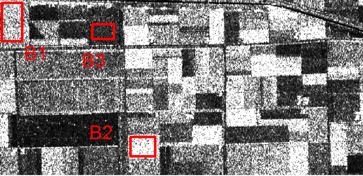
Table I lists the ML parameter estimates as well as the sample sizes. Each sample is taken from a single class without evidence of texture. Notice that the estimates for the equivalent number of looks are very close, although lower than the nominal value. We also show the determinant of the estimated covariance matrix. This quantity, called geometric intensity in [50], is the generalized variance in multivariate analysis; it can be used as a measure of mean backscatter [51]. According to it, region B2 presents the highest return, followed by B1 and by B3; this is in agreement with what is observed in channel HH, cf. Fig. 1.
| Regions | # pixels | ||||
|---|---|---|---|---|---|
| . | |||||
| . | |||||
| . | |||||
Fig. 2 depicts the empirical densities of data from the agricultural regions along with the fitted marginal densities. The scaled Wishart density collapses to the Gamma density:
| (4) |
where , is the element of , and is the -th entry of . In practice, represents the mean polarization channel . Figs. 2(a)-2(c) show the data and the densities for the estimated number of looks (black curve) and the fixed value (gray curve). These densities are remarkably close, and also to the histograms, so the Gamma assumption is reasonable.
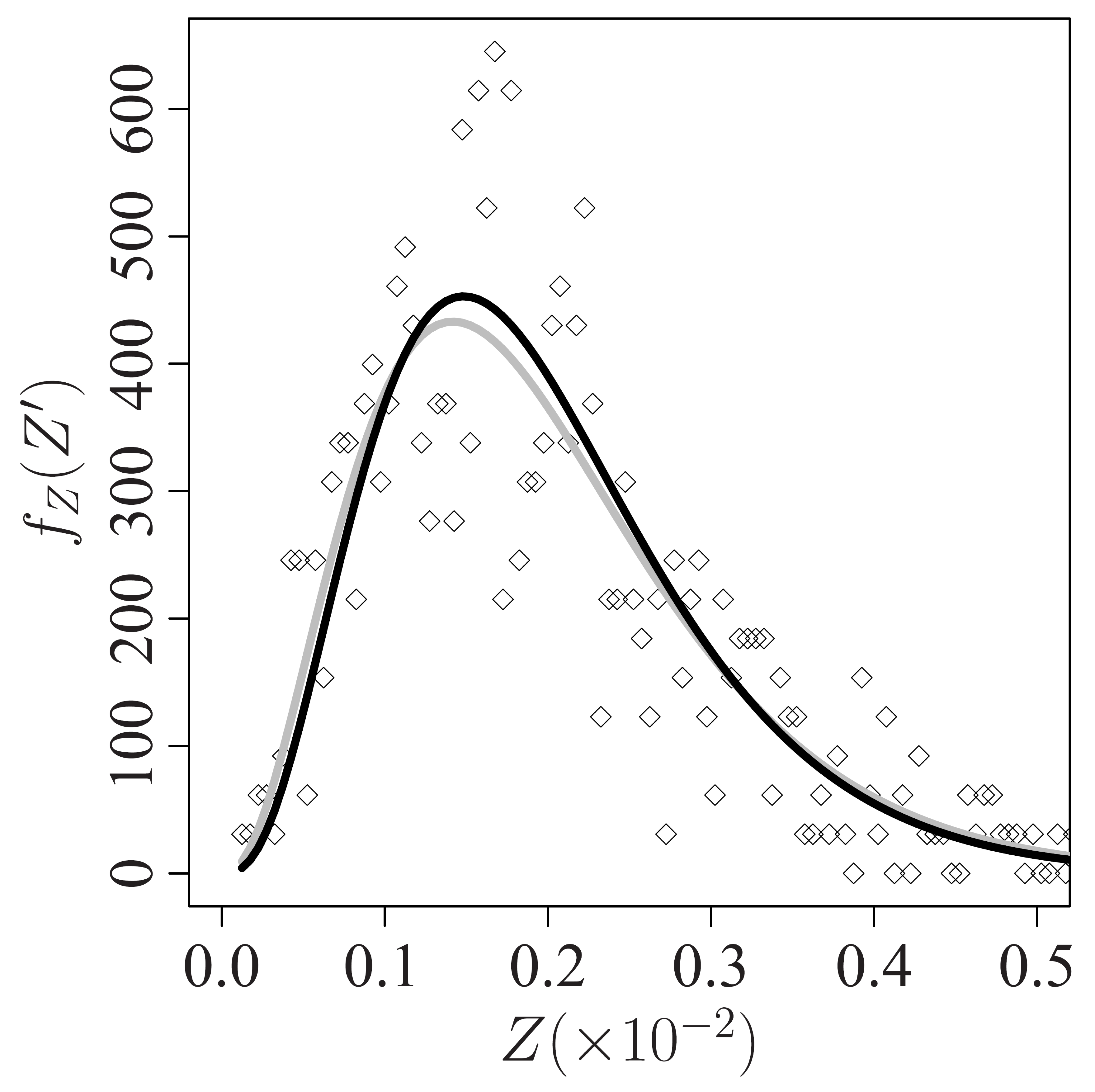
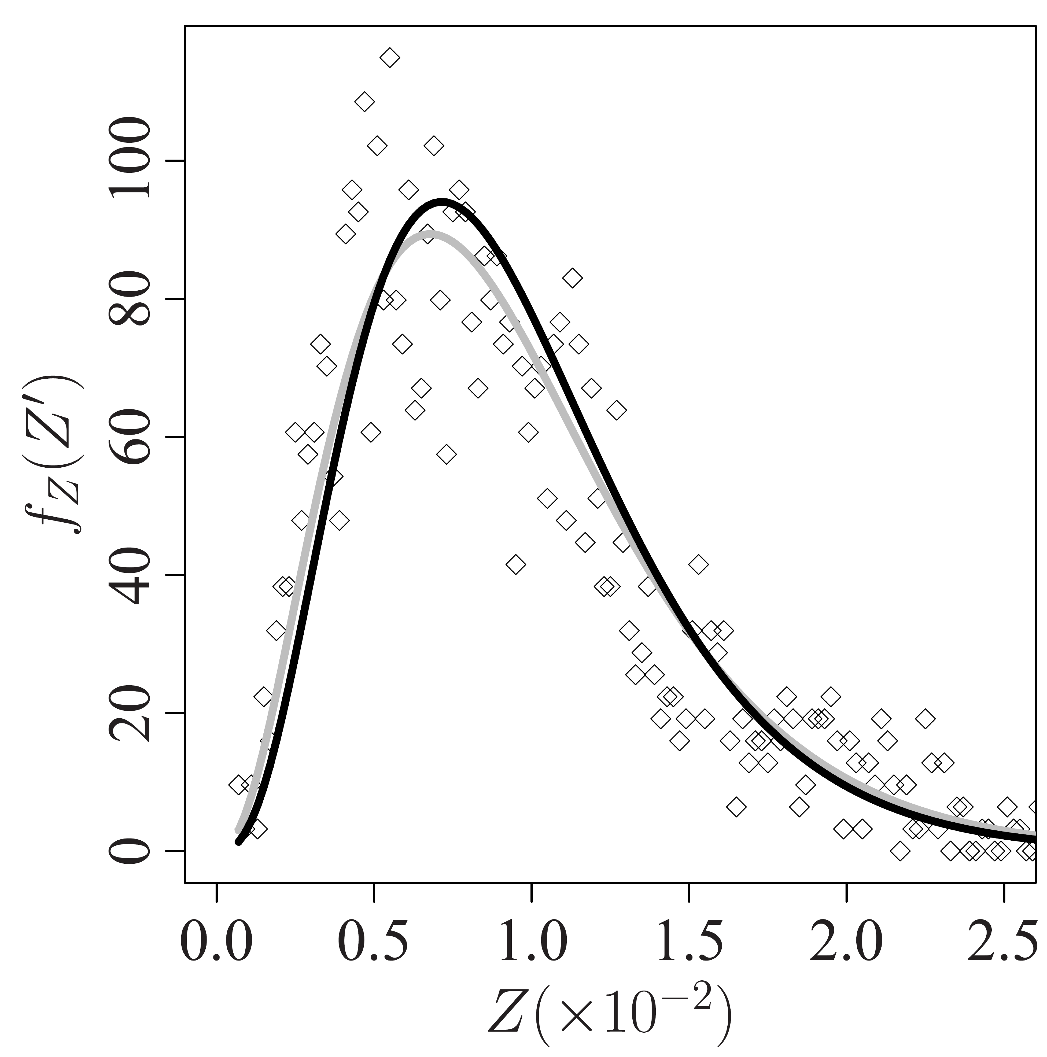
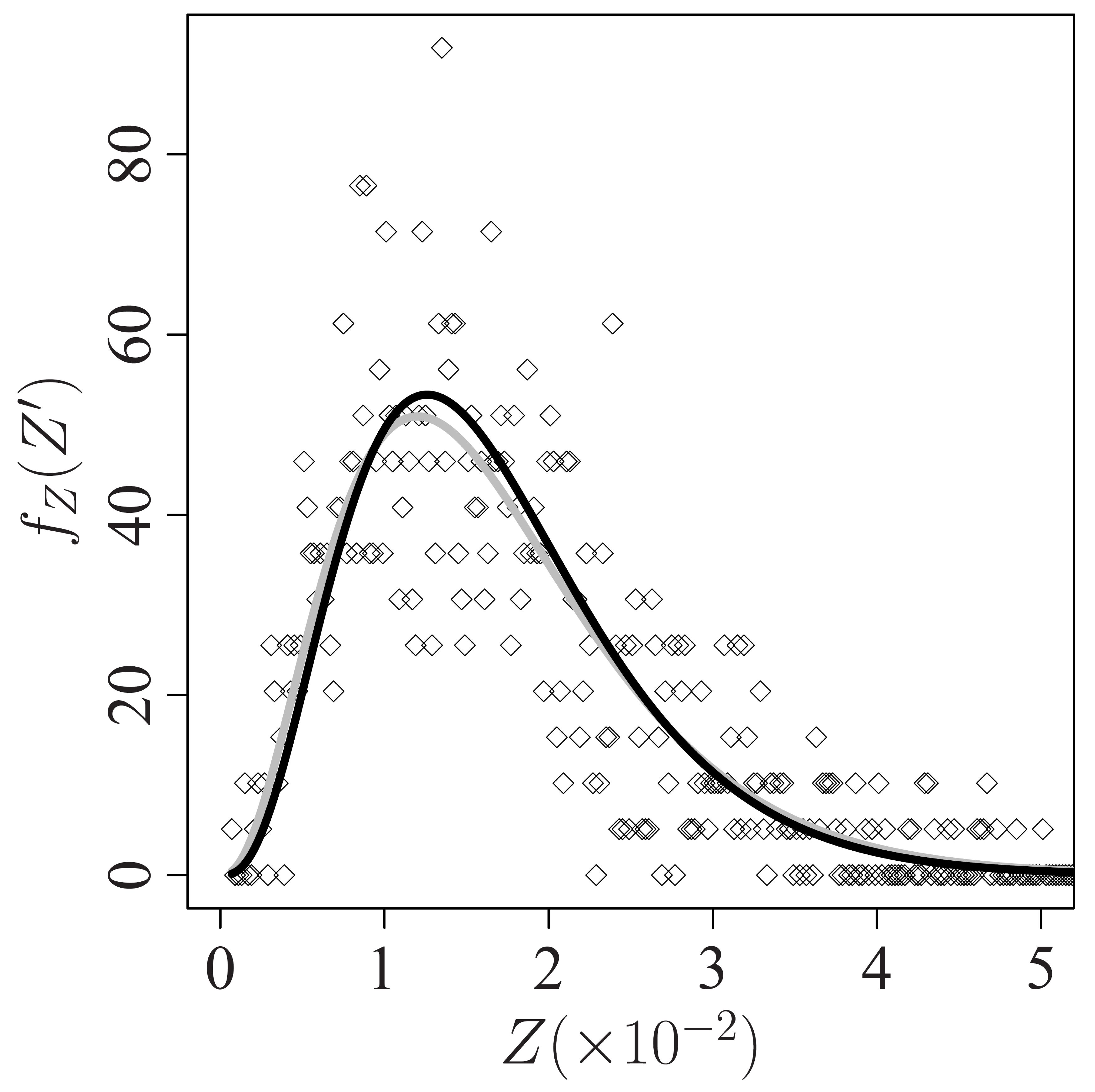
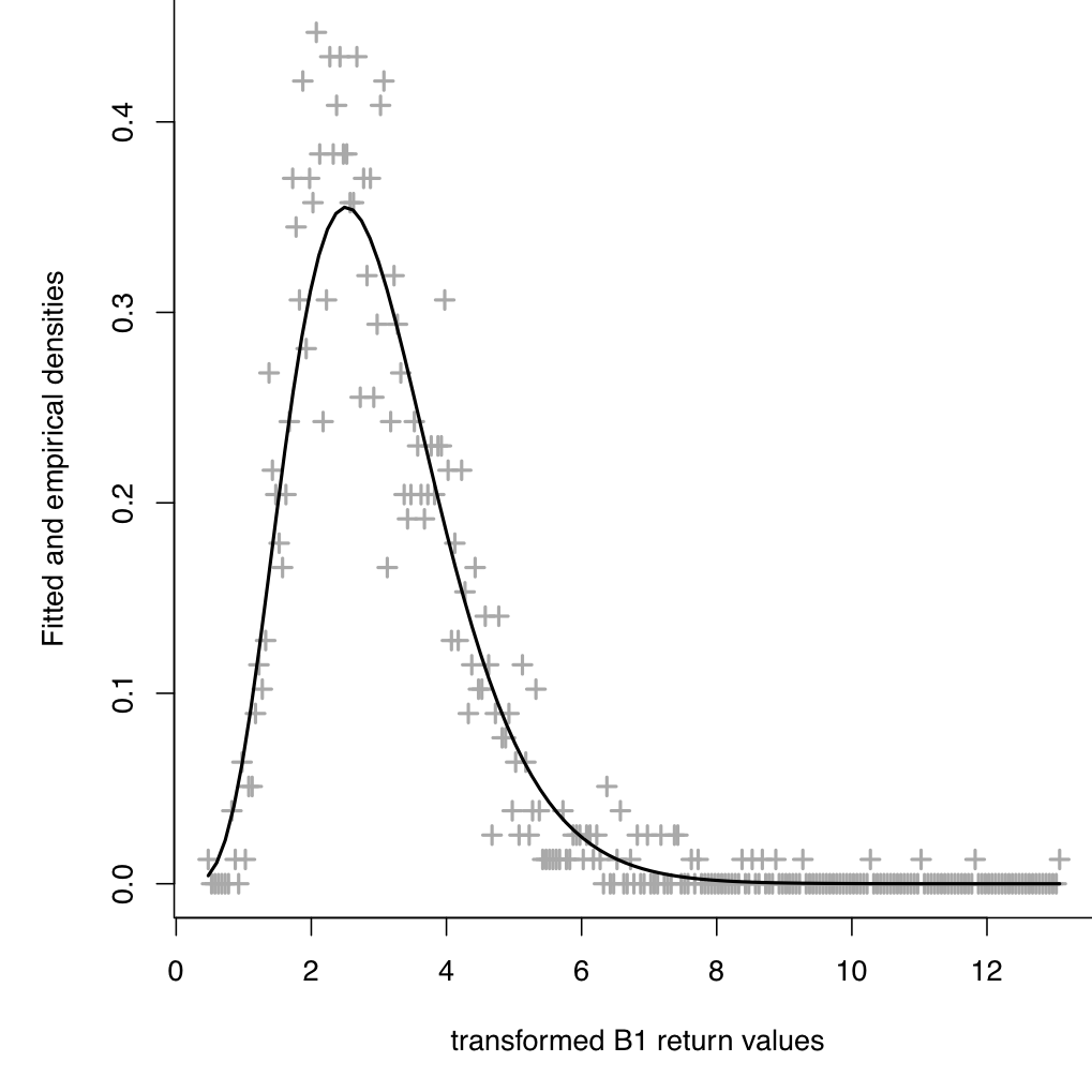
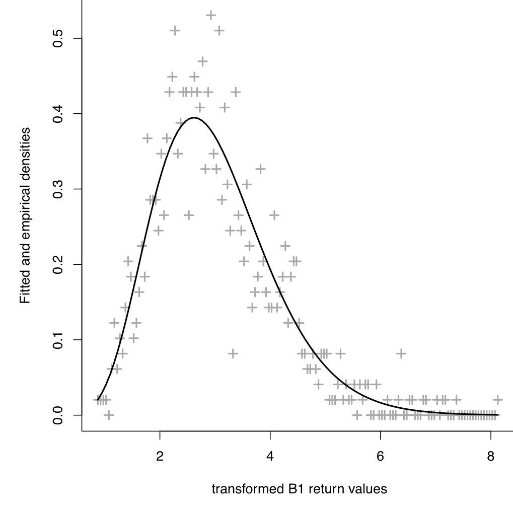
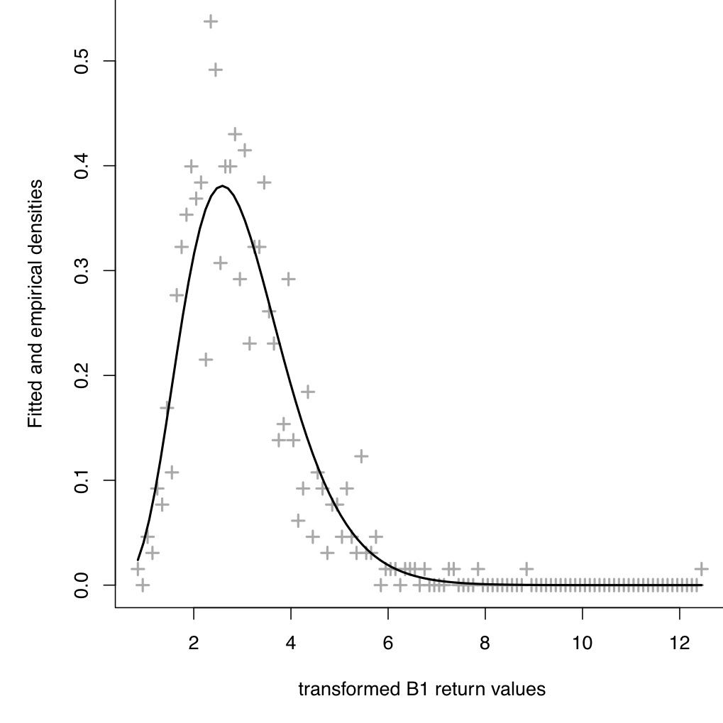
According to Akbari et al. [52], if is a random sample drawn from and represents the maximum likelihood estimator of , then follows a Gamma distribution for . Fig. 3 displays fitted and empirical densities of such transformed data for the three selected regions. These results indicate that data may follow a scaled complex Wishart model. Additionally, the Kolmogorov-Smirnov statistic -values for checking the adequacy of the Gamma model to the transformed data are , , and for regions B1, B2, and B3, respectively.
We used likelihood ratio tests for two and three samples in order to quantify the similarity among these samples, The results presented in Table II point out that is different from and , but these last two are similar. Although a visual inspection of areas B2 and B3 (Fig. 1) suggests regions of different nature, their observations projected via are statistically similar.
| Statistics | -value | |
|---|---|---|
These samples are used to validate our proposed methods in Section IV.
III Hypothesis tests in PolSAR Data: A Survey
This section provides a survey concerning three hypothesis tests which have been studied in the PolSAR data literature.
We assume that PolSAR data follow a scaled complex Wishart distribution. Change detection is often formulated as a statistical test for assuming known.
The two main approaches in the literature are: (i) likelihood ratio [11] and (ii) stochastic distances [27]. In this paper, the former proposal is extended to the context of scaled complex Wishart distributions, since the original approach used the nonscaled Wishart law. Moreover, this paper also introduces an alternative way for validating by means of entropy measures [26]. Subsequently, these methodologies are introduced and discussed. In order to obtain more general results, we will provide expressions for testing .
III-A Likelihood Ratio Statistics
The log-likelihood ratio (LR) statistic has great importance in inference on parametric models. Let be the LR statistic for assessing the simple null hypothesis . As discussed in [53], such statistic based on has an asymptotic distribution , where is the difference between the dimensions of the parameter spaces under the alternative and the null hypotheses. We denote such spaces by and , respectively.
Let and be two random samples from and of sizes and , respectively. The LR statistic is given by
where , , and . Thus, we have that
| (5) |
and
where and represent the number of looks and covariance matrix under the null hypothesis, respectively. Akbari et al. [42] discuss the two-sample LR test under the model.
Sections III-B and -C discuss tests for based on information-theoretic measures.
III-B The Kullback-Leibler distance
The Kullback-Leibler divergence () is one of oldest discrepancy measures between stochastic models; it has a central role in Information Theory [54]. This quantity was firstly understood as a measure of the error in choosing a model when another is the true one. It has been used in image processing for segmentation [55], classification [56], boundary detection [57, 58], and change detection [23]. Moreover, has a close relationship with the Neyman-Pearson lemma [54], and its symmetrization has been suggested as a correction form for another important goodness-of-fit measure for comparing statistical models: the Akaike information criterion [59].
Let and be two random matrices defined over the common support of positive definite complex matrices of size . The Kullback-Leibler distance is defined by
with differential element given by
where is the -th entry of matrix ; and and denote the real and imaginary part operators, respectively [43].
When distances are taken between particular cases of the same distribution, only the parameters are relevant. In this case, the parameters and replace the random variables and .
Salicrú et al. [60] proposed a hypothesis test based on . Let and be the ML estimators for and based on random samples of size and , respectively. Under the regularity conditions discussed in [60, p. 380], the following lemma holds.
Lemma 1
If and , then
| (6) |
where “” denotes convergence in distribution.
Proposition 1
Let and and be ML estimates obtained from two sufficiently large random samples of sizes and , respectively; then the null hypothesis can be rejected at level if .
Frery et al. [27] presented closed expressions for when the random matrices and follow the Wishart distribution:
| (7) |
from which the test statistic follows.
III-C Shannon and Rényi Entropies
The Shannon entropy has achieved a prominent position in PolSAR imagery. Morio et al. [61] applied it for extracting features from polarimetric targets, assuming the circular Gaussian distribution. The Shannon entropy has also been used for classifying PolSAR textures [62, 63]. In the subsequent discussion, we present a comprehensive examination of hypothesis tests based on Shannon and Rényi entropies.
Let be a pdf with parameter vector . The Shannon and Rényi (with order ) entropies are defined, respectively, as:
| (8) | ||||
| and | ||||
| (9) |
Pardo et al. [64] derived an important result which paves the way for asymptotic statistical inference methods based on entropies.
Lemma 2
Let be the ML estimate of the parameter vector based on an -point random sample from a model having pdf . Then
where , is the Gaussian distribution with mean and variance ,
| (10) |
is the Fisher information matrix, and such that for .
Now we introduce a methodology for hypothesis tests and confidence intervals based on entropies. We aim at testing the following hypotheses:
where . In other words, is there any statistical evidence for rejecting the assumption that two PolSAR samples come from the same model?
Let be the ML estimate for based on a random sample of size from for and . From Lemma 2, we have that
where
Then we obtain the following test statistic:
| (11) |
the expressions for and are presented the Appendix. We are now in position to state the following result.
Proposition 2
Let , , be sufficiently large. If , then the null hypothesis can be rejected at a level if .
Whereas tests based on stochastic distances, such as , allow contrasting only two samples, those based on entropies permit assessing samples at once; cf. (11). For issues involving more than two populations ( in (11)), this is a major advantage of the latter over the former. In the case of comparing two samples of the same size, i.e. and , (11) reduces to
IV Performance Analysis
In this section we assess the performance of the methodologies proposed with three experiments involving simulated (under the scaled Wishart complex law) and actual PolSAR data. Firstly, we use Monte Carlo experiments to measure (i) test size (false alarm rate) and (ii) test power (). For the test size, we check whether two samples from are from the same distribution, i.e., in a scenario where there was no change and there might be false positives. We assess the test power checking if two samples from and , for , are correctly identified as a situation where there was a change. We then perform two experiments with actual PolSAR data.
IV-A Simulated Data
We compare the following hypothesis tests:
-
•
Likelihood ratio ;
-
•
Kullback-Leibler distance ;
-
•
Statistics based on Shannon and Rényi entropies.
We fixed , since this value was found in Ref. [26] to provide good discrimination in hard-to-deal-with situations. We assume that the number of looks is known, as in [11, 25]. Therefore, we are able to compare information-theoretic measures with the methodology proposed by Conradsen et al. [11].
The samples are generated according to Algorithm 1.
The parameters used for assessing the null hypothesis are , and (12), the sample covariance matrix of area B1, Fig. 1. As we are interested in the behavior of the tests with small sample sizes, we computed the size of the hypothesis at for .
Let be the number of Monte Carlo replications and the number of occurrences under (i.e., pairs of samples are taken from the same model) on which the null hypothesis is rejected at the nominal level . The empirical test size (ETS) or false positive rate is defined by . We used , as suggested in [25], and did not suffer expressive changes for larger values.
| (12) |
Table III shows: (i) the empirical test size at nominal levels , , , and (ii) the mean test statistic () of the four statistics.
| Mean values | ||||
| Likelihood ratio () | ||||
| Shannon Entropy () | ||||
| Rényi Entropy () | ||||
| Kullback-Leibler Distance () | ||||
In average, all test statistics behave as expected when the sample sizes increase: and tend to one, while and tend to nine. Recall that the asymptotic distribution of the two former is , while the two latter are .
The and tests exhibit the closest empirical sizes to the nominal levels, as confirmed by Fig. 4. The ETS associated with and are biased, however the bias reduces as the sample size increases. We conclude that these two statistics require larger sample sizes to achieve the expected asymptotic behavior.
In general terms, Table III suggests this inequality:
| (13) |
The size of tests (False Positive rates) based on the Shannon entropy and likelihood ratio are the closest to the nominal level.


We also studied the test power. We wish to reject the hypothesis given two samples drawn from and where ; i.e, under . The rate , where is the number of rejections of under , estimates the Type II error or false negative [19], and we aim at quantifying the test power .
Fig. 5 presents the estimated power for several samples sizes. The test based on Shannon entropy performs best. In this case, we obtain the inequality:
The relation between discriminatory powers within groups and has been discussed in the statistical literature. This fact can be explained twofold, namely (i) the relationship between the Neyman and Pearson lemma and the Kullback-Leibler distance [54], and (ii) the fact that [65].
The best test statistics should have both empirical size near to the nominal level, and the highest estimated power. Thus, based on this evidence and on the estimated size, we suggest as the best discriminator on scenarios which follow the scaled complex Wishart distribution.


IV-B Experiments with Data from Sensors
In this section we apply the proposed test statistics to two studies: (i) for assessing to the data presented in Fig. 1 (single date) and (ii) for detecting changes on two PolSAR images captured at different instants, as displayed in Fig. 8 (multitemporal data). ENL is assumed constant.
IV-B1 Single date experiment
Our first experiment aims at assessing , the empirical test size (Type I error or Probability of False Alarm), using pairs of disjoint samples from the same target.
This experiment is outlined in Algorithm 2. We used samples of size .
Fig. 6 shows the observed . Inequality (13) is also verified on actual data. For , and ; i.e., all tests overestimate , but and presented better results than and . For B2 and B3, , overcoming , and .
PolSAR regions are Wishart, our explanation for the better performance of is deviations from this hypothesis.
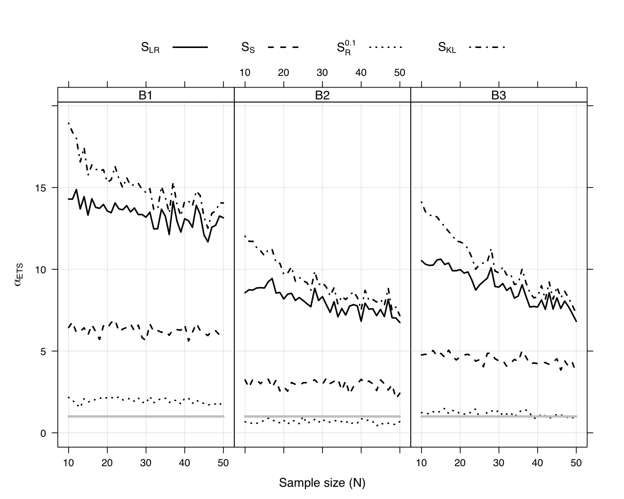
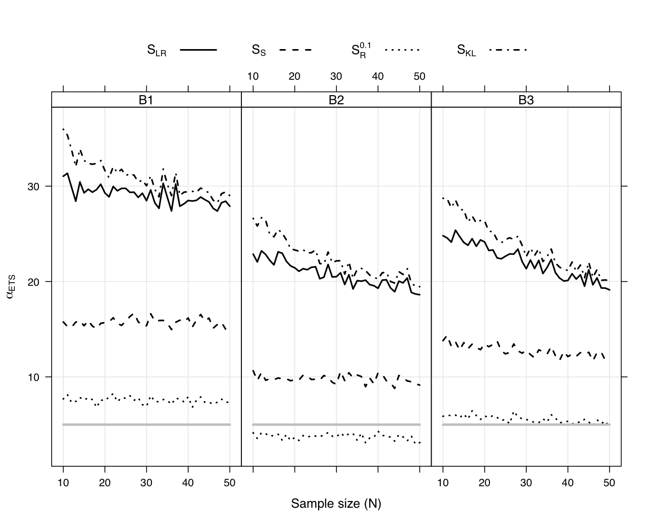
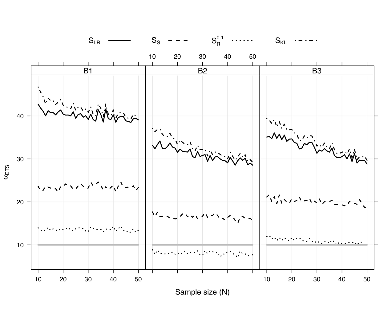
These results present evidence that the test statistics based on outperforms the other ones. This test presented good results even for small samples. Thus, this measure is suggested as a relevant change detection tool for PolSAR imagery.
IV-B2 Multitemporal data
Fig. 7 presents the study areas for this experiment: surroundings of the city of Los Angeles, CA, USA. These pictures refer to a dense urban area whose changes are caused by the urbanization process. Ratha et al. [30] employed these data in the proposal of change detectors for single look polarimetric data using a geodesic distance. Here we apply the four multilook PolSAR data detectors discussed in Section III. Fig. 8 shows the Pauli decomposition of two UAVSAR images obtained by JPL’s UAVSAR (Uninhabited Aerial Vehicle Synthetic Aperture Radar) sensor at two different instants (23 April 2009, and 3 May 2015).
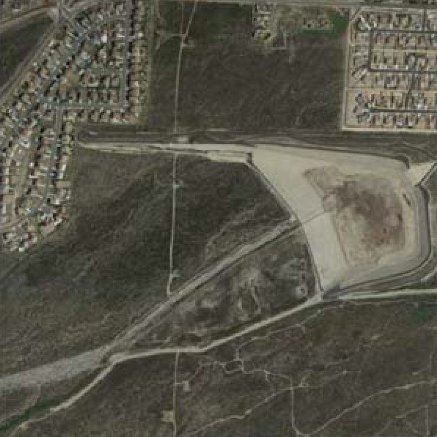
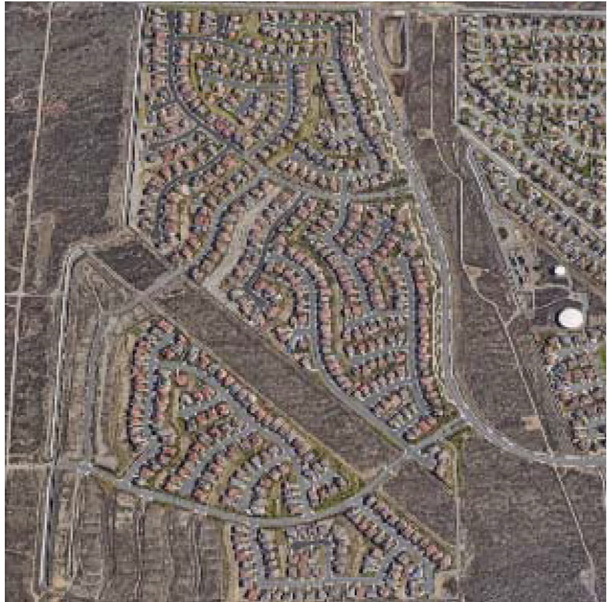
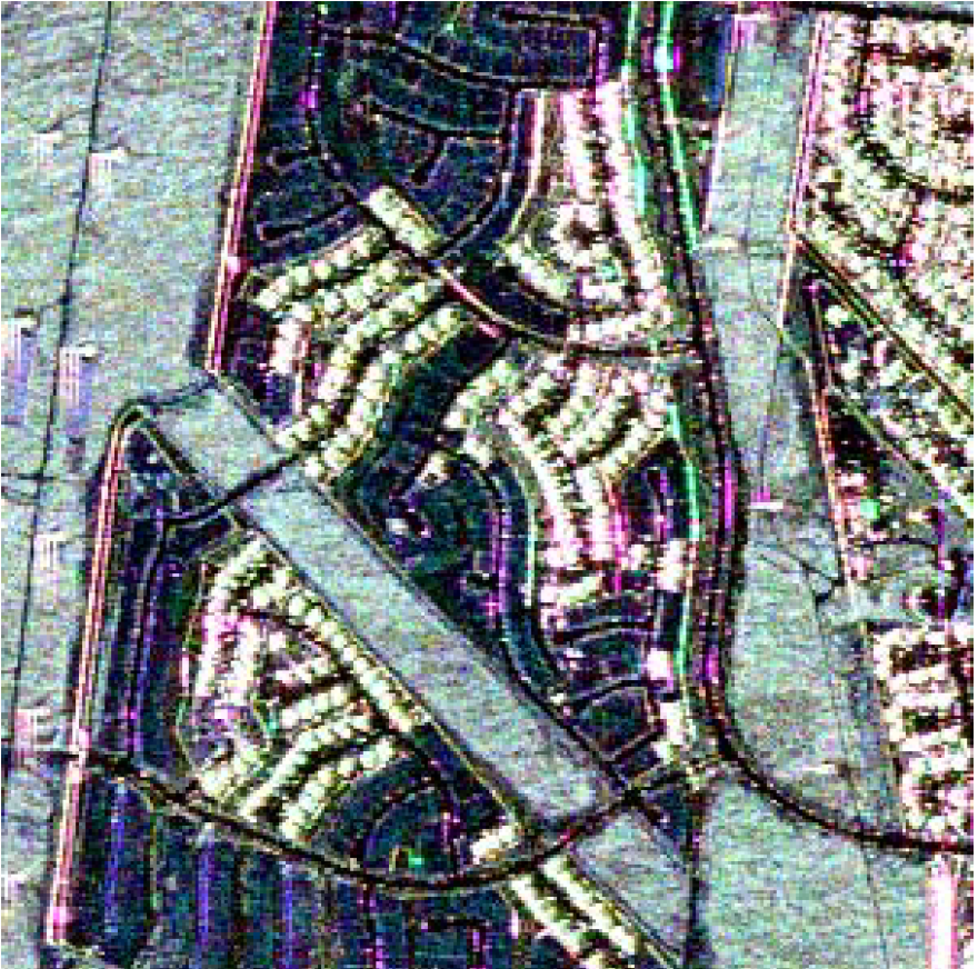
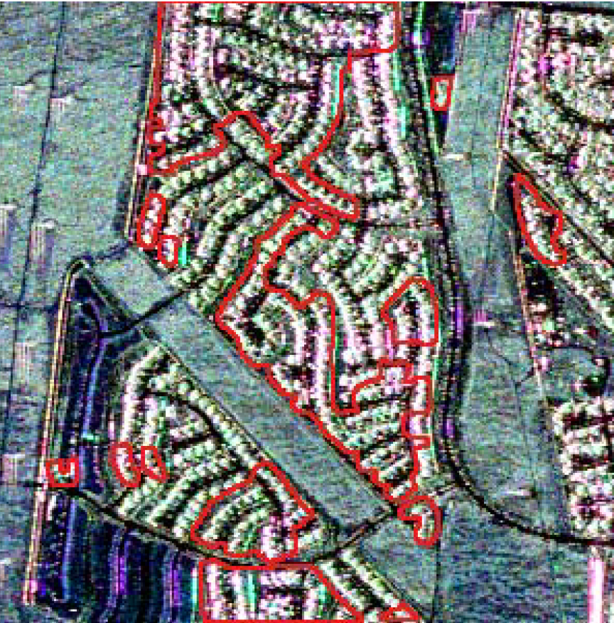
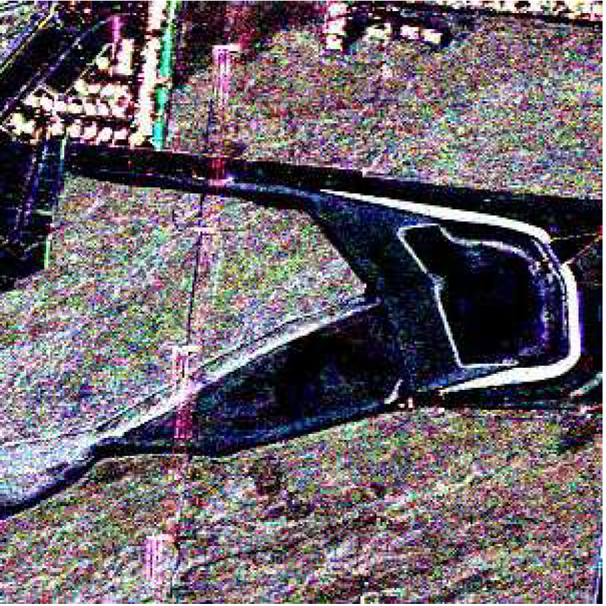
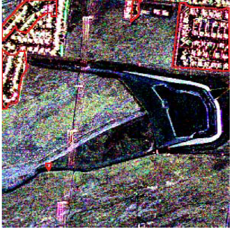
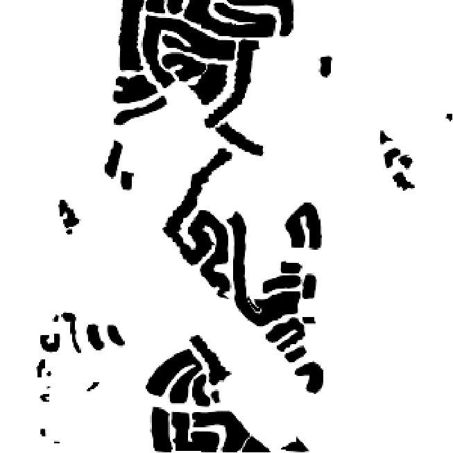
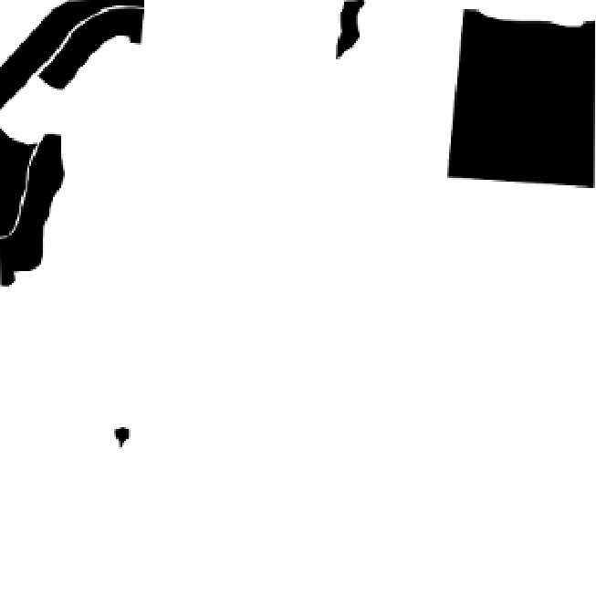
Using windows of size on both dates, we computed the , , , and test statistics and, from them, -value maps; cf. Figs. 9 and 10. Probability values higher than are drawn in black, as they provide no evidence of change. Values below range vary from red to dark blue (from strong to weak evidence of change).
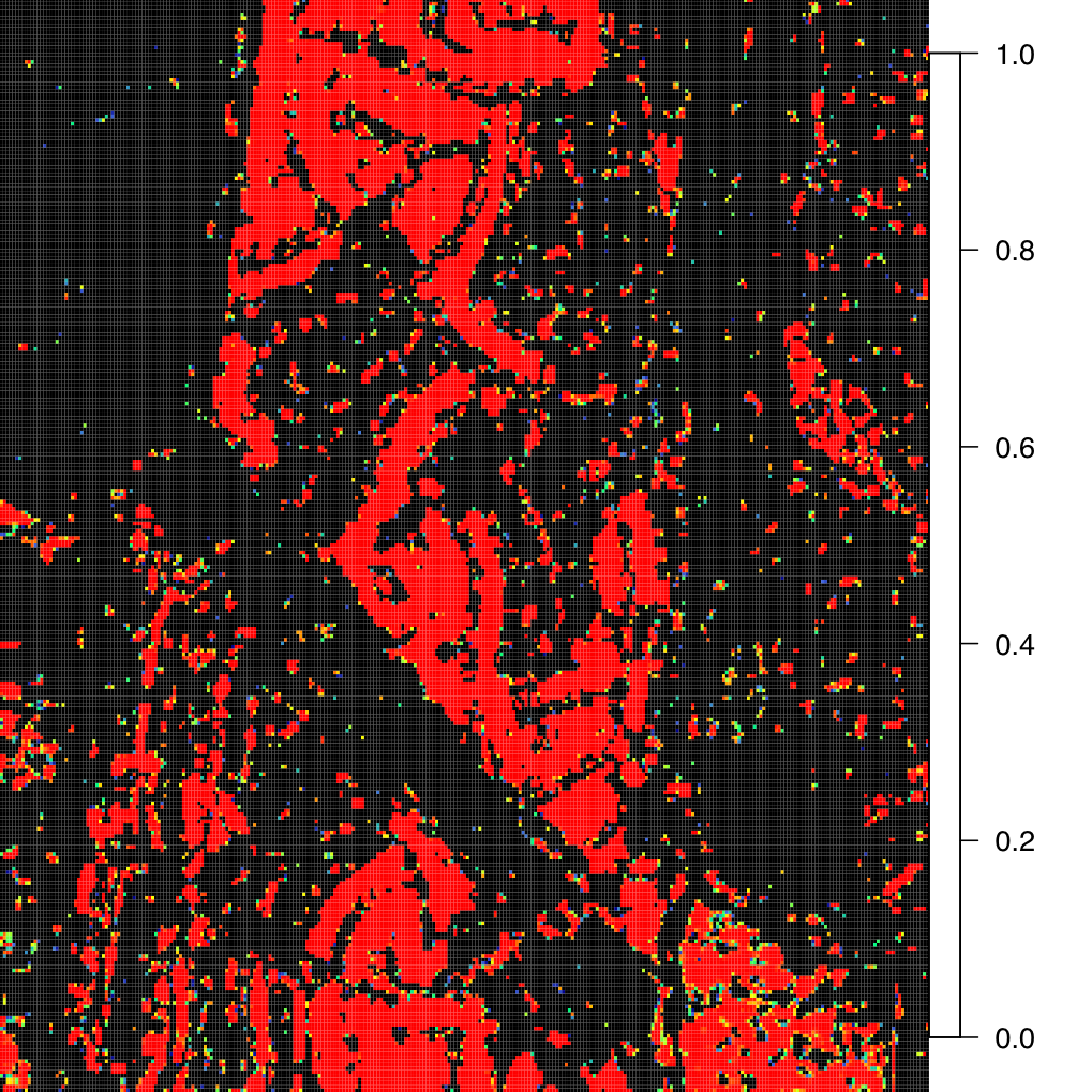
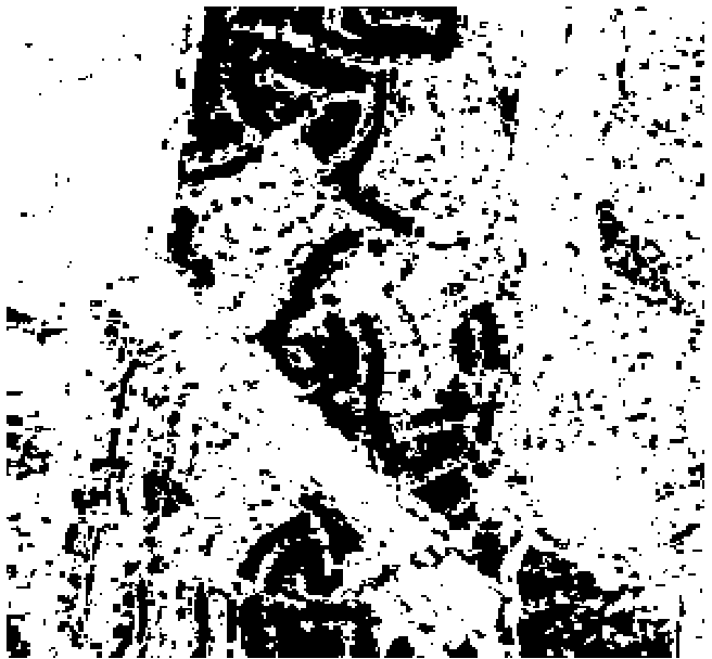
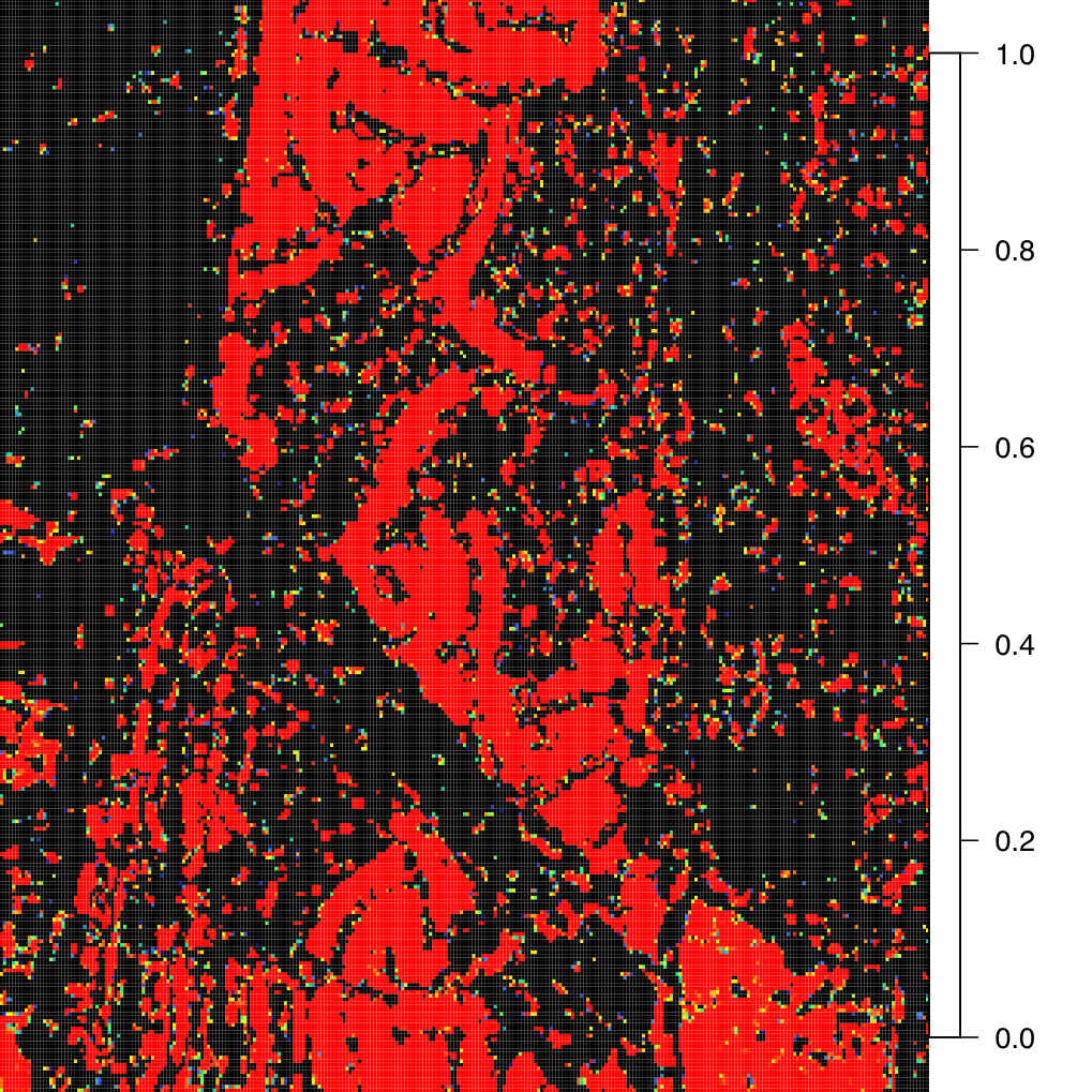
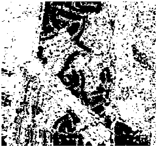
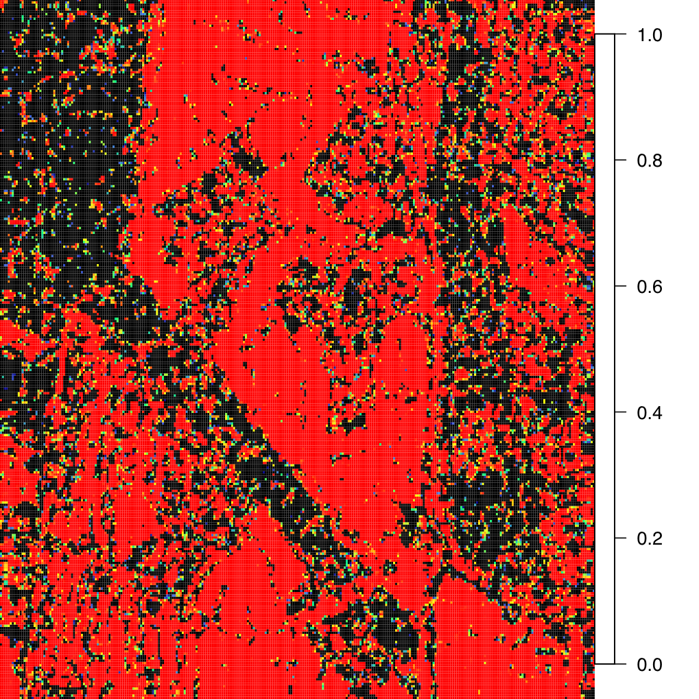
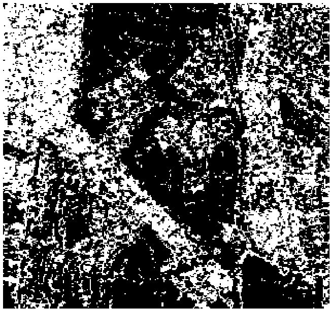
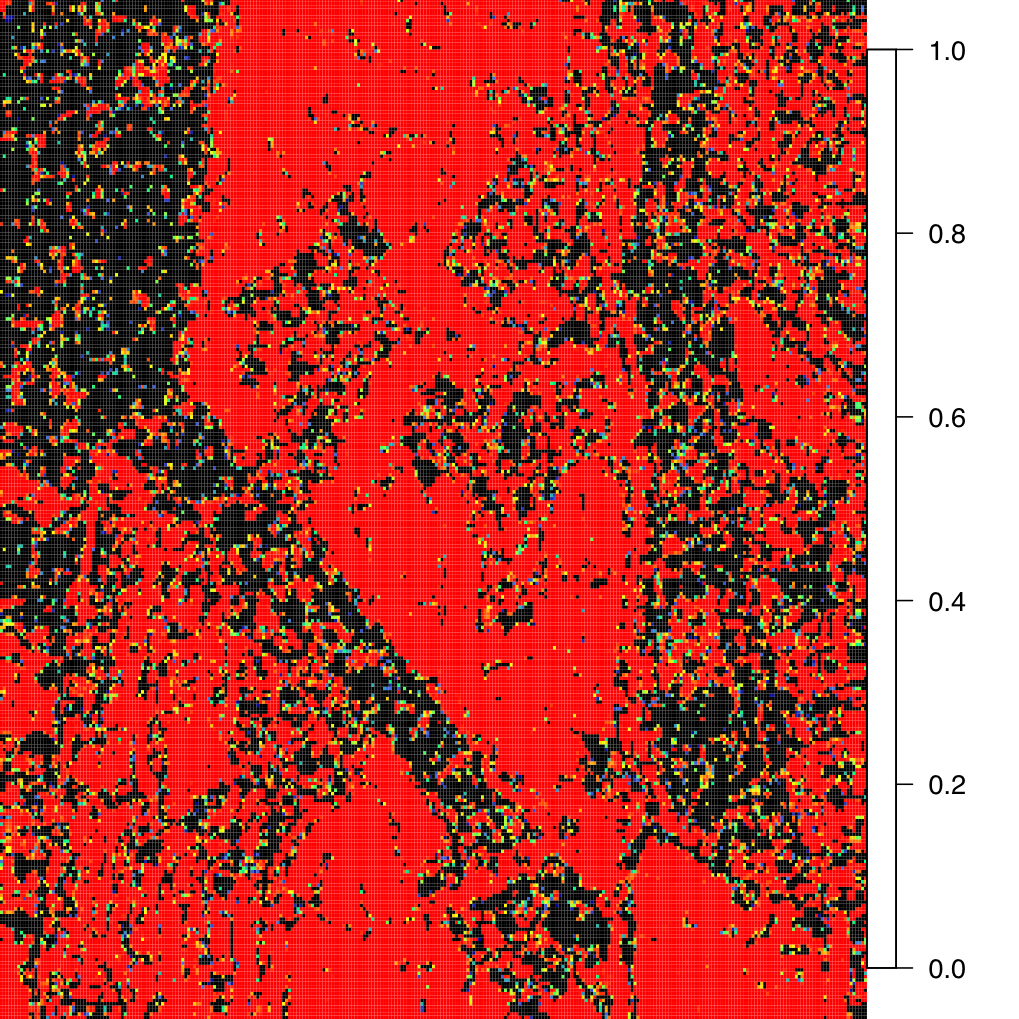
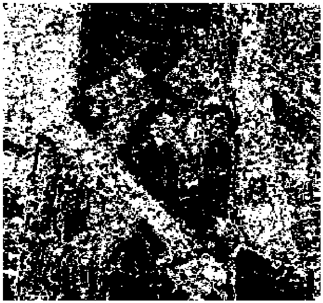
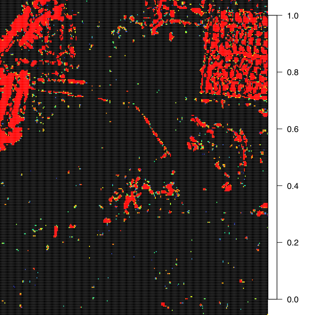
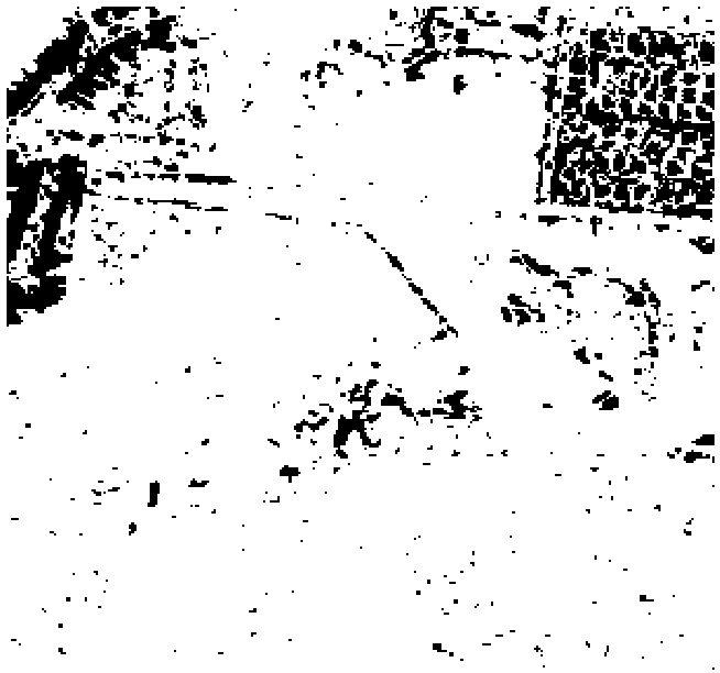
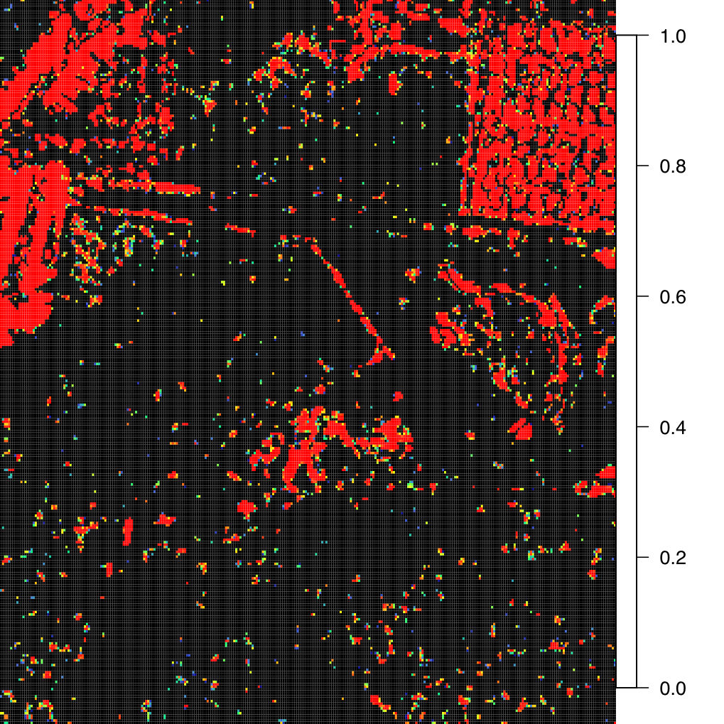
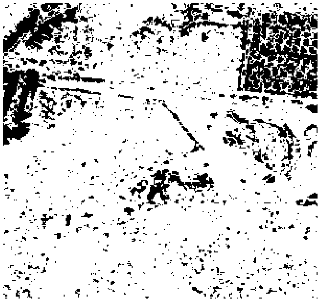
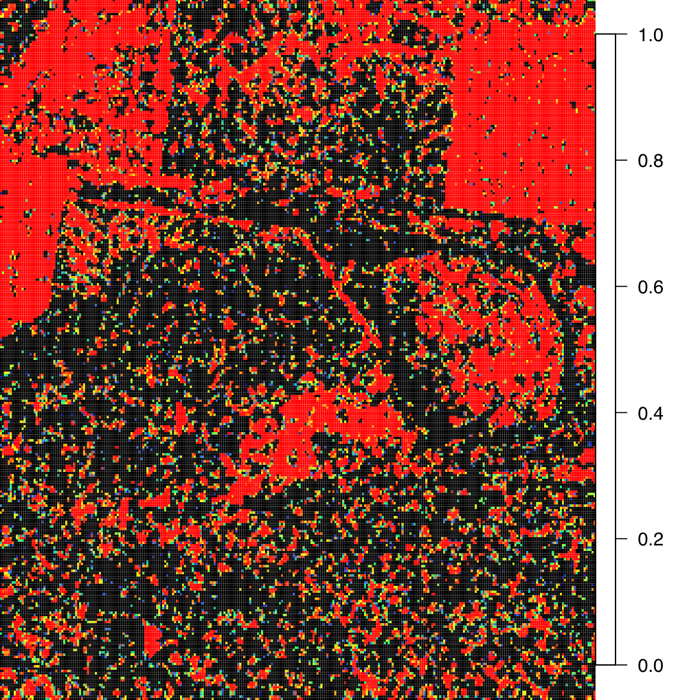


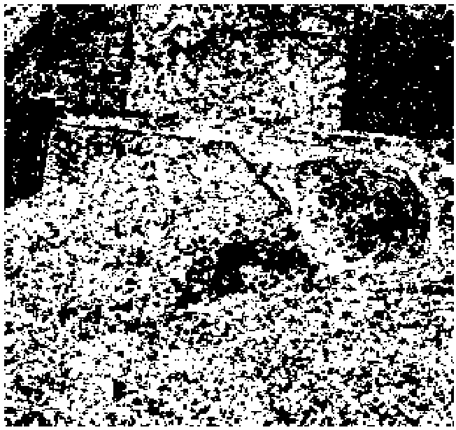
It is noticeable that and are similar, cf. Figs. 9(a), 10(a) and 9(c), 10(c), while and look alike, see Figs. 9(e), 10(e), 9(g), and 10(g), but somewhat different from the previous pair.
Fig. 11 shows the relationship between and for the second scene, along with the identity function for reference. The -values associated to the Shannon statistic are smaller than that those related to the Rényi statistic, so the former tends to reject more than , as discussed in the simulation experiments.

Finally, Figs. 9(b), 9(d), 9(f), 9(h) and 10(b), 10(d), 10(f), 10(h) show binary images resulting from thresholding the , , , and statistics for the first and second scenes: -values larger than are shown in white, otherwise in black. The results, again, favor entropy-based detectors.
To confirm the qualitative discussion, we quantify the performance of detectors with respect to reference maps in Figs 8(e)-8(f) in terms of five measures:
-
•
False positive (FP): Number of pixels indicated as change by Reference map (RM), but classified as no change;
-
•
False negative (FN): Number of pixels indicated as no change by RM, but classified as change;
-
•
False alarm rate (FA): , where is the number of unchanged pixels according to the detector;
-
•
Detection rate (DR): , where TP is the number of pixels indicated as change by both RM and the detector, and CG is the number of changed pixels according to the detector; and
-
•
Kappa coefficient: , where and where is the proportion of pixels under the condition relative to the total number of pixels and TN is the number of pixels indicated as no change by both RM and the detector.
The reference maps were prepared by specialists with Bing and Google Earth imagery; cf. Ref. [30].
Table IV shows the results. obtained the best performance, followed by , for both data sets with respect to and DR. These detectors presented lower FN and FA than and . and performed better than entropy-based detectors with respect to FP. The values of FP were smaller than in all cases, so this is not an issue for any detector.
| Detectors | FP (%) | FN (%) | FA (%) | DR(%) | (%) |
|---|---|---|---|---|---|
| Scene 1 | |||||
| 0.060 | 13.433 | 13.493 | 20.408 | 24.597 | |
| 0.052 | 14.055 | 14.107 | 19.765 | 23.023 | |
| 0.343 | 5.476 | 5.819 | 35.387 | 52.482 | |
| 0.431 | 3.709 | 4.140 | 42.988 | 62.272 | |
| Scene 2 | |||||
| 0.104 | 9.551 | 9.655 | 20.964 | 25.552 | |
| 0.094 | 10.404 | 10.497 | 19.682 | 23.087 | |
| 0.739 | 2.568 | 3.307 | 41.598 | 52.598 | |
| 0.920 | 1.254 | 2.174 | 55.590 | 62.519 | |
V Conclusions
We quantified and compared the performance of four change detection methods for fully polarimetric SAR data. These methods are based on the likelihood-ratio statistic, on the Kullback-Leibler distance, and on the Rényi and Shannon entropies. We used empirical test powers and sizes as comparison criteria.
Firstly, the performance of the methods was quantified through a Monte Carlo study using scenarios modeled by the scaled complex Wishart law. The empirical test sizes showed evidence that the detectors based on the likelihood ratio and Shannon entropy statistics presented the best performance. In particular, the one based on the entropy is the best for small samples and statistically similar to the . Additionally, the tests based on the Kullback-Leibler and on the likelihood ratio statistics tend to overestimate the nominal level, while those which employ entropies underestimate it.
Regarding the empirical test power, the test based on the Shannon entropy presented, in a consistent fashion, the best results. Computational costs are quite different. The test statistic based on the likelihood ratio requires evaluating (5), while depends only on the Kullback-Leibler distance (7). The latter is less demanding than the former by an order of magnitude. Thus, on those situations in which and are competitive (for moderate and large sample sizes), the Kullback-Leibler test is more attractive because it has the lowest computational cost.
Secondly, and since estimated test sizes were quite competitive, two experiments with actual data were performed. For the single date experiment, in all the situations considered, the test based on Rényi entropy with order presented the best results. The multitemporal data experiments suggests that change detectors equipped by entropies provide better performance than those based on the Kullback-Leibler distance and those based on the likelihood ratio statistic. Finally, the diversity of tests statistics stemming from Information Theory opens the venue for investigation of composite decision rules, as in Ref. [66].
Appendix A Derivation outline of expressions for Shannon and Rényi statistics
Under the scaled complex Wishart law, Frery et al. [26] derived the following variances:
-
•
Shannon:
(16) -
•
Rényi entropy:
(17)
References
- [1] J. S. Lee and E. Pottier, Polarimetric Radar Imaging: From Basics to Applications. Boca Raton: CRC, 2009.
- [2] D. Lu, P. Mausel, E. Brondízio, and E. Moran, “Change detection techniques,” International Journal of Remote Sensing, vol. 25, no. 12, pp. 2365–2401, Apr. 2004.
- [3] E. J. M. Rignot and J. J. Van Zyl, “Change detection techniques for ERS-1 SAR data,” IEEE Transactions on Geoscience and Remote Sensing, vol. 31, no. 4, pp. 896–906, Jul. 1993.
- [4] C. Oliver and S. Quegan, Understanding Synthetic Aperture Radar Images, ser. The SciTech Radar and Defense series. SciTech Publishing, 1998.
- [5] G. Liu, L. Jiao, F. Liu, H. Zhong, and S. Wang, “A new patch based change detector for polarimetric SAR data,” Pattern Recognition, vol. 48, no. 3, pp. 685–695, Mar. 2015.
- [6] G. Moser, S. Serpico, and G. Vernazza, “Unsupervised change detection from multichannel SAR images,” IEEE Geoscience and Remote Sensing Letters, vol. 4, no. 2, pp. 278–282, Apr. 2007.
- [7] T. T. Lê, A. M. Atto, E. Trouvão, A. Solikhin, and V. Pinel, “Change detection matrix for multitemporal filtering and change analysis of SAR and PolSAR image time series,” ISPRS Journal of Photogrammetry and Remote Sensing, vol. 107, pp. 64–76, Sep. 2015.
- [8] F. Melgani and S. B. Serpico, “A statistical approach to the fusion of spectral and spatio-temporal contextual information for the classification of remote-sensing images,” Pattern Recognition Letters, vol. 23, no. 9, pp. 1053–1061, Jul. 2002.
- [9] A. M. Atto, E. Trouve, Y. Berthoumieu, and G. Mercier, “Multidate divergence matrices for the analysis of SAR image time series,” IEEE Transactions on Geoscience and Remote Sensing, vol. 51, no. 4, pp. 1922–1938, Apr. 2013.
- [10] M. Silva, F. Cribari-Neto, and A. C. Frery, “Improved likelihood inference for the roughness parameter of the GA0 distribution,” Environmetrics, vol. 19, no. 4, pp. 347–368, Aug. 2008.
- [11] K. Conradsen, A. A. Nielsen, J. Schou, and H. Skriver, “A test statistic in the complex Wishart distribution and its application to change detection in polarimetric SAR data,” IEEE Transactions on Geoscience and Remote Sensing, vol. 41, no. 1, pp. 4–19, Feb. 2003.
- [12] V. Akbari, S. N. Anfinsen, A. P. Doulgeris, and T. Eltoft, “The Hotelling-Lawley trace statistic for change detection in polarimetric SAR data under the complex Wishart distribution,” in IEEE International Geoscience and Remote Sensing Symposium (IGARSS’2013), Jul. 2013, pp. 4162–4165.
- [13] M. Liu, H. Zhang, C. Wang, and F. Wu, “Change detection of multilook polarimetric SAR images using heterogeneous clutter models,” IEEE Transactions on Geoscience and Remote Sensing, vol. 52, no. 12, pp. 7483–7494, Dec. 2014.
- [14] V. Carotenuto, A. De Maio, C. Clemente, and J. Soraghan, “Invariant rules for multipolarization SAR change detection,” IEEE Transactions on Geoscience and Remote Sensing, vol. 53, no. 6, pp. 3294–3311, Jun. 2015.
- [15] V. Carotenuto, A. De Maio, C. Clemente, J. J. Soraghan, and G. Alfano, “Forcing scale-invariance in multi-polarization SAR change detection,” IEEE Transactions on Geoscience and Remote Sensing, vol. 54, no. 1, pp. 36–50, Jan. 2016.
- [16] V. Carotenuto, A. De Maio, C. Clemente, and J. Soraghan, “Unstructured versus structured GLRT for multipolarization SAR change detection,” IEEE Geoscience and Remote Sensing Letters, vol. 12, no. 8, pp. 1665–1669, Aug. 2015.
- [17] M. Liu, H. Zhang, C. Wang, Y. Tang, B. Zhang, F. Wu, T. Wu, and X. Chen, “Polarimetric synthetic aperture radar change detection for specific land cover types,” International Journal of Digital Earth, vol. 8, no. 4, pp. 334–344, Jan. 2015.
- [18] A. Nielsen, K. Conradsen, and H. Skriver, “Change detection in full and dual polarization, single- and multifrequency SAR data,” IEEE Journal of Selected Topics in Applied Earth Observations and Remote Sensing, vol. 8, no. 8, pp. 4041–4048, Aug. 2015.
- [19] K. Conradsen, A. A. Nielsen, and H. Skriver, “Determining the points of change in time series of polarimetric SAR data,” IEEE Transactions on Geoscience and Remote Sensing, vol. 54, no. 5, pp. 3007–3024, May 2016.
- [20] K.-F. Lin and D. Perissin, “Identification of statistically homogeneous pixels based on one-sample test,” Remote Sensing, vol. 37, no. 1, pp. 1–13, Jan. 2017.
- [21] G. Moser and S. Serpico, “Generalized minimum-error thresholding for unsupervised change detection from SAR amplitude imagery,” IEEE Transactions on Geoscience and Remote Sensing, vol. 44, no. 10, pp. 2972–2982, Oct. 2006.
- [22] A. Marino and I. Hajnsek, “A change detector based on an optimization with polarimetric SAR imagery,” IEEE Transactions on Geoscience and Remote Sensing, vol. 52, no. 8, pp. 4781–4798, Aug. 2014.
- [23] J. Inglada and G. Mercier, “A new statistical similarity measure for change detection in multitemporal SAR images and its extension to multiscale change analysis,” IEEE Transactions on Geoscience and Remote Sensing, vol. 45, no. 5, pp. 1432–1445, May 2007.
- [24] G. Mercier, G. Moser, and S. Serpico, “Conditional copulas for change detection in heterogeneous remote sensing images,” IEEE Transactions on Geoscience and Remote Sensing, vol. 46, no. 5, pp. 1428–1441, May 2008.
- [25] A. D. C. Nascimento, R. J. Cintra, and A. C. Frery, “Hypothesis testing in speckled data with stochastic distances,” IEEE Transactions on Geoscience and Remote Sensing, vol. 48, no. 1, pp. 373–385, Jan. 2010.
- [26] A. C. Frery, R. J. Cintra, and A. D. C. Nascimento, “Entropy-based statistical analysis of PolSAR data,” IEEE Transactions on Geoscience and Remote Sensing, vol. 51, no. 6, pp. 3733–3743, Jun. 2013.
- [27] A. C. Frery, A. D. C. Nascimento, and R. J. Cintra, “Analytic expressions for stochastic distances between relaxed complex Wishart distributions,” IEEE Transactions on Geoscience and Remote Sensing, vol. 52, no. 2, pp. 1213–1226, Feb. 2014.
- [28] A. Marino, S. R. Cloude, and J. M. Lopez-Sanchez, “A new polarimetric change detector in radar imagery,” IEEE Transactions on Geoscience and Remote Sensing, vol. 51, no. 5, pp. 2986–3000, May 2013.
- [29] Y. Zheng, X. Zhang, B. Hou, and G. Liu, “Using combined difference image and k-means clustering for SAR image change detection,” IEEE Geoscience and Remote Sensing Letters, vol. 11, no. 3, pp. 691–695, Mar. 2014.
- [30] D. Ratha, S. De, T. Celik, and A. Bhattacharya, “Change detection in polarimetric SAR images using a geodesic distance between scattering mechanisms,” IEEE Geoscience and Remote Sensing Letters, vol. 14, no. 7, pp. 1066 – 1070, Jul. 2017.
- [31] V. Akbari, A. P. Doulgeris, and T. Eltoft, “Monitoring glacier changes using multitemporal multipolarization SAR images,” IEEE Transactions on Geoscience and Remote Sensing, vol. 52, no. 6, pp. 3729–3741, Jun. 2014.
- [32] R. Radke, S. Andra, O. Al-Kofahi, and B. Roysam, “Image change detection algorithms: a systematic survey,” IEEE Transactions on Image Processing, vol. 14, no. 3, pp. 294–307, Mar. 2005.
- [33] J. Schou, H. Skriver, A. H. Nielsen, and K. Conradsen, “CFAR edge detector for polarimetric SAR images,” IEEE Transactions on Geoscience and Remote Sensing, vol. 41, no. 1, pp. 20–32, Jan. 2003.
- [34] P. R. Kersten, J. S. Lee, and T. L. Ainsworth, “A comparison of change detection statistics in PolSAR images,” in IEEE International Geoscience and Remote Sensing Symposium (IGARSS’2005), Jul. 2005, pp. 4836–4839.
- [35] M. Molinier and Y. Rauste, “Comparison and evaluation of polarimetric change detection techniques in aerial SAR data,” in IEEE International Geoscience and Remote Sensing Symposium (IGARSS’2007), Jul. 2007, pp. 2386–2389.
- [36] V. Akbari, S. N. Anfinsen, A. P. Doulgeris, T. Eltoft, G. Moser, and S. B. Serpico, “Polarimetric SAR change detection with the complex Hotelling-Lawley trace statistic,” IEEE Transactions on Geoscience and Remote Sensing, vol. 54, no. 7, pp. 3953–3966, Jul. 2016.
- [37] K. D. Ward, “Compound representation of high resolution sea clutter,” Electronics Letters, vol. 17, no. 16, pp. 561–563, Aug. 1981.
- [38] E. Erten, A. Reigber, L. Ferro-Famil, and O. Hellwich, “A new coherent similarity measure for temporal multichannel scene characterization,” IEEE Transactions on Geoscience and Remote Sensing, vol. 50, no. 7, pp. 2839–2851, Jul. 2012.
- [39] A. C. Frery, H. J. Muller, C. C. F. Yanasse, and S. J. S. Sant’Anna, “A model for extremely heterogeneous clutter,” IEEE Transactions on Geoscience and Remote Sensing, vol. 35, no. 3, pp. 648–659, May 1997.
- [40] A. D. C. Nascimento, M. M. Horta, A. C. Frery, and R. J. Cintra, “Comparing edge detection methods based on stochastic entropies and distances for PolSAR imagery,” IEEE Journal of Selected Topics in Applied Earth Observations and Remote Sensing, vol. 7, no. 2, pp. 648–663, Feb. 2014.
- [41] L. Torres, S. J. S. Sant’Anna, C. C. Freitas, and A. C. Frery, “Speckle reduction in polarimetric SAR imagery with stochastic distances and nonlocal means,” Pattern Recognition, vol. 47, no. 1, pp. 141–157, Apr. 2014.
- [42] V. Akbari, S. N. Anfinsen, A. P. Doulgeris, and T. Eltoft, “A change detector for polarimetric SAR data based on the relaxed Wishart distribution,” in IEEE International Geoscience and Remote Sensing Symposium (IGARSS’2015), Jul. 2015, pp. 3806–3809.
- [43] N. R. Goodman, “Statistical analysis based on a certain complex Gaussian distribution (an introduction),” The Annals of Mathematical Statistics, vol. 34, no. 1, pp. 152–177, 1963.
- [44] C. López-Martínez, X. Fábregas, and E. Pottier, “Multidimensional speckle noise model,” EURASIP Journal on Applied Signal Processing, vol. 2005, no. 20, pp. 3259–3271, Dec. 2005.
- [45] S. N. Anfinsen, A. P. Doulgeris, and T. Eltoft, “Estimation of the equivalent number of looks in polarimetric synthetic aperture radar imagery,” IEEE Transactions on Geoscience and Remote Sensing, vol. 47, no. 11, pp. 3795–3809, Nov. 2009.
- [46] S. N. Anfinsen, T. Eltoft, and A. P. Doulgeris, “A relaxed Wishart model for polarimetric SAR data,” in Proceedings of the 4th International Workshop on Science and Applications of SAR Polarimetry and Polarimetric Interferometry (POLinSAR’2009), Frascati, Italy, 2009.
- [47] M. Abramowitz and I. A. Stegun, Handbook of Mathematical Functions With Formulas, Graphs, and Mathematical Tables, t. G. p. ninth Dover printing, Ed. Dover, 1964.
- [48] J. E. Gentle, Elements of Computational Statistics, ser. Statistics and computing. Springer, 2002.
- [49] A. P. Doulgeris, S. N. Anfinsen, and T. Eltoft, “Automated non-Gaussian clustering of polarimetric synthetic aperture radar images,” IEEE Transactions on Geoscience and Remote Sensing, vol. 49, no. 10, pp. 3665–3676, Oct. 2011.
- [50] S. Skrunes, C. Brekke, and T. Eltoft, “Characterization of marine surface slicks by Radarsat-2 multipolarization features,” IEEE Transactions on Geoscience and Remote Sensing, vol. 52, no. 9, pp. 5302–5319, Sep. 2014.
- [51] N. R. Goodman, “The distribution of determinant of a complex Wishart distributed matrix,” The Annals of Mathematical Statistics, vol. 34, no. 1, pp. 178–180, 1963.
- [52] V. Akbari, A. P. Doulgeri, G. Moser, T. Eltoft, S. N. Anfinsen, and S. B. Serpico, “A textural-contextual model for unsupervised segmentation of multipolarization synthetic aperture radar images,” IEEE Transactions on Geoscience and Remote Sensing, vol. 51, no. 4, pp. 2442–2453, Apr. 2013.
- [53] G. Casella and R. L. Berger, Statistical Inference. Duxbury Press, 2002.
- [54] S. Eguchi and J. Copas, “Interpreting Kullback-Leibler divergence with the Neyman-Pearson lemma,” Journal of Multivariate Analysis, vol. 97, no. 9, pp. 2034–2040, Oct. 2006.
- [55] J. M. Beaulieu and R. Touzi, “Segmentation of textured polarimetric SAR scenes by likelihood approximation,” IEEE Transactions on Geoscience and Remote Sensing, vol. 42, no. 10, pp. 2063–2072, Oct. 2004.
- [56] P. R. Kersten, J. S. Lee, and T. L. Ainsworth, “Unsupervised classification of polarimetric synthetic aperture radar images using fuzzy clustering and EM clustering,” IEEE Transactions on Geoscience and Remote Sensing, vol. 43, no. 3, pp. 519–527, Mar. 2005.
- [57] A. C. Frery, J. Jacobo-Berlles, J. Gambini, and M. Mejail, “Polarimetric SAR image segmentation with B-splines and a new statistical model,” Multidimensional Systems and Signal Processing, vol. 21, no. 4, pp. 319–342, Dec. 2010.
- [58] J. Gambini, M. Mejail, J. Jacobo-Berlles, and A. C. Frery, “Accuracy of edge detection methods with local information in speckled imagery,” Statistics and Computing, vol. 18, no. 1, pp. 15–26, Mar. 2008.
- [59] A. K. Seghouane and S. I. Amari, “The AIC criterion and symmetrizing the Kullback-Leibler divergence,” IEEE Transactions on Neural Networks, vol. 18, no. 1, pp. 97–106, Jan. 2007.
- [60] M. Salicrú, M. L. Menéndez, L. Pardo, and D. Morales, “On the applications of divergence type measures in testing statistical hypothesis,” Journal of Multivariate Analysis, vol. 51, no. 2, pp. 372–391, Feb. 1994.
- [61] J. Morio, P. Réfrégier, F. Goudail, P. C. Dubois Fernandez, and X. Dupuis, “A characterization of Shannon entropy and Bhattacharyya measure of contrast in polarimetric and interferometric SAR image,” Proceedings of the IEEE, vol. 97, no. 6, pp. 1097–1108, Jun. 2009.
- [62] S. R. Cloude and E. Pottier, “An entropy based classification scheme for land application of polarimetric SAR,” IEEE Transactions on Geoscience and Remote Sensing, vol. 35, no. 1, pp. 68–78, Jan. 1997.
- [63] W. Yan, W. Yang, Y. Liu, and H. Sun, “Unsupervised classification of PolinSAR image based on Shannon entropy characterization,” in IEEE International Conference on Signal Processing (ICSP’2010), 2010, pp. 2192 –2195.
- [64] L. Pardo, D. Morales, M. Salicrú, and M. L. Menéndez, “Large sample behavior of entropy measures when parameters are estimated,” Communications in Statistics - Theory and Methods, vol. 26, no. 2, pp. 483–501, Jan. 1997.
- [65] T. M. Cover and J. A. Thomas, Elements of Information Theory. New York: Wiley-Interscience, 1991.
- [66] G. P. Silva Junior, A. C. Frery, S. Sandri, H. Bustince, E. Barrenechea, and C. Marco-Detchart, “Optical images-based edge detection in Synthetic Aperture Radar images,” Knowledge-Based Systems, vol. 87, pp. 38–46, Aug. 2015.
- [67] X. Deng, C. López-Martínez, J. Chen, and P. Han, “Statistical modeling of polarimetric SAR data: A survey and challenges,” Remote Sensing, vol. 9, no. 4, p. 348, Apr. 2017.
![[Uncaptioned image]](/html/1801.08901/assets/x1.png) |
Abraão D. C. Nascimento holds B.Sc. M.Sc. and D.Sc. degrees in Statistics from Universidade Federal de Pernambuco (UFPE), Brazil, in 2005, 2007, and 2012, respectively. In 2014, he joined the Department of Statistics at UFPE as Adjoint Professor. His research interests are statistical information theory, inference on random matrices (with emphasis for applications on PolSAR imagery), statistical theory of shape, spatio-temporal processes, survival analysis, and asymptotic theory. |
![[Uncaptioned image]](/html/1801.08901/assets/x2.png) |
Alejandro C. Frery (S’92–SM’03) received the B.Sc. degree in Electronic and Electrical Engineering from the Universidad de Mendoza, Mendoza, Argentina. His M.Sc. degree was in Applied Mathematics (Statistics) from the Instituto de Matemática Pura e Aplicada (IMPA, Rio de Janeiro) and his Ph.D. degree was in Applied Computing from the Instituto Nacional de Pesquisas Espaciais (INPE, São José dos Campos, Brazil). He is currently the leader of LaCCAN – Laboratório de Computação Científica e Análise Numérica, Universidade Federal de Alagoas, Maceió, Brazil. His research interests are statistical computing and stochastic modelling. |
![[Uncaptioned image]](/html/1801.08901/assets/Renato.png) |
Renato J. Cintra (S’00, M’05, SM’10) received the B.Sc., M.Sc., and D.Sc. degrees in electrical engineering from the Universidade Federal de Pernambuco (UFPE), Recife, Brazil, in 1999, 2001, and 2005, respectively. He joined the Department of Statistics, UFPE, in 2005. In 2014–2015, he was visiting professor at the Département Informatique, INSA, Lyon, France. During 2017–2018, he is a visiting professor at the University of Calgary, Canada. He is an associate editor for IEEE Geoscience and Remote Sensing Letters; Springer Circuits, Systems, and Signal Processing; IET Circuits, Devices & Systems; and Journal of Communication and Information Systems. His long-term topics of research include: approximation theory for discrete transforms, theory and methods for digital signal processing, and statistical methods. |