Strongly consistent autoregressive predictors in abstract Banach spaces

Summary

This work derives new results on strong consistent estimation and prediction for autoregressive processes of order 1 in a separable Banach space B. The consistency results are obtained for the componentwise estimator of the autocorrelation operator in the norm of the space $\mathcal{L}(B)$ of bounded linear operators on B. The strong consistency of the associated plug–in predictor then follows in the $B$-norm. A Gelfand triple is defined through the Hilbert space constructed in Kuelbs’ Lemma Kuelbs [1970]. A Hilbert–Schmidt embedding introduces the Reproducing Kernel Hilbert space (RKHS), generated by the autocovariance operator, into the Hilbert space conforming the Rigged Hilbert space structure. This paper extends the work of Bosq [2000] and Labbas and Mourid [2002].

In press, manuscript accepted in Journal of Multivariate Analysis

Key words: ARB(1) processes; Banach spaces; Continuous embeddings; Functional plug-in predictors; Strongly consistent estimators.

1 Introduction

In the last few decades, there exists a growing interest on the statistical analysis of high–dimensional data, from the Functional Data Analysis (FDA) perspective. The book by Ramsay and Silverman [2005] provides an overview on FDA techniques, extended from the multivariate data context, or specifically formulated for the FDA framework. The monograph by Hsing and Eubank [2015] introduces functional analytical tools usually applied in the estimation of random elements in function spaces. The book by Horváth and Kokoszka [2012] is mainly concerned with inference based on second order statistics. A central topic in this book is the analysis of functional data, displaying dependent structures in time and space. The methodological survey paper by Cuevas [2014], on the state of the art in FDA, discusses central topics in FDA. Recent advances in the statistical analysis of high–dimensional data, from the parametric, semiparametric and nonparametric FDA frameworks, are collected in the Special Issue by Goia and Vieu [2016].

Linear time series models traditionally arise for processing temporal linear correlated data. In the FDA context, the monograph by Bosq [2000] introduces linear functional time series theory. The RKHS, generated by the autocovariance operator, plays a crucial role in the estimation approach presented in this monograph. In particular, the eigenvectors of the autocovariance operator are considered for projection (see also Álvarez-Liébana [2017]). Its empirical version is computed, when they are unknown. The resulting plug–in predictor is obtained as a linear functional of the observations, based on the empirical approximation of the autocorrelation operator. This approach exploits the Hilbert space structure, and its extension to the metric space context, and, in particular, to the Banach space context, requires to deriving a relationship (continuous embeddings) between the Banach space norm, and the RKHS norm, induced by the autocovariance operator, in contrast with the nonparametric regression approach for functional prediction (see, for instance, Ferraty et al. [2012], where asymptotic normality is derived). Specifically, in the nonparametric approach, a linear combination of the observed response values is usually considered. That is the case of the nonparametric local–weighting–based approach, involving weights defined from an isotropic kernel, depending on the metric or semi–metric of the space, where the regressors take their values (see, for example, Ferraty and Vieu [2006]; see also Ferraty et al. [2002], in the functional time series framework). The nonparametric approach is then more flexible regarding the structure of the space where the functional values of the regressors lie (usually a semi–metric space is considered). However, some computational drawbacks are present in its implementation, requiring the resolution of several selection problems. For instance, a choice of the smoothing parameter, and the kernel involved, in the definition of the weights, should be performed. Real–valued covariates were incorporated in the novel semiparametric kernel–based proposal by Aneiros-Pérez and Vieu [2008], involving an extension to the functional partial linear time series framework (see also Aneiros-Pérez and Vieu [2006]). Goia and Vieu [2015] also adopt a semi–parametric approach in their formulation of a two–terms Partitioned Functional Single Index Model. Geenens [2011] exploits the alternative provided by semi–metrics to avoid the curse of infinite dimensionality of some functional estimators.

On the other hand, in a parametric linear framework, Mas and Pumo [2010] introduced functional time series models in Banach spaces. In particular, strong mixing conditions and the absolute regularity of Banach–valued autoregressive processes have been studied in Allam and Mourid [2001]. Empirical estimators for Banach–valued autoregressive processes are studied in Bosq [2002], where, under some regularity conditions, and for the case of orthogonal innovations, the empirical mean is proved to be asymptotically optimal, with respect to almost surely (a.s.) convergence, and convergence of order two. The empirical autocovariance operator was also interpreted as a sample mean of an autoregressive process in a suitable space of linear operators. The extension of these results to the case of weakly dependent innovations is obtained in Dehling and Sharipov [2005]. A strongly–consistent sieve estimator of the autocorrelation operator of a Banach–valued autoregressive process is considered in Rachedi and Mourid [2003]. Limit theorems for a seasonality estimator, in the case of Banach autoregressive perturbations, are formulated in Mourid [2002]. Confidence regions for the periodic seasonality function, in the Banach space of continuous functions, is obtained as well. An approximation of Parzen’s optimal predictor, in the RKHS framework, is applied in Mokhtari and Mourid [2003], for prediction of temporal stochastic process in Banach spaces. The existence and uniqueness of an almost surely strictly periodically correlated solution, to the first order autoregressive model in Banach spaces, is derived in Parvardeh et al. [2017]. Under some regularity conditions, limit results are obtained for AR$\mathcal{D}$(1) processes in Hajj [2011], where $\mathcal{D}=\mathcal{D}([0,1])$ denotes the Skorokhod space of right–continuous functions on $[0,1],$ having limit to the left at each $t\in[0,1].$ Conditions for the existence of strictly stationary solutions of ARMA equations in Banach spaces, with independent and identically distributed noise innovations, are derived in Spangenberg [2013].

In the derivation of strong–consistency results for ARB(1) componentwise estimators and predictors, Bosq [2000] restricts his attention to the case of the Banach space $\mathcal{C}([0,1])$ of continuous functions on $[0,1],$ with the supremum norm. Labbas and Mourid [2002] considers an ARB(1) context, for $B$ being an arbitrary real separable Banach space, under the construction of a Hilbert space $\widetilde{H},$ where $B$ is continuously embedded, as given in the Kuelbs’s Lemma in [Kuelbs, 1970, Lemma 2.1]. Under the existence of a continuous extension to $\widetilde{H}$ of the autocorrelation operator $\rho\in\mathcal{L}(B),$ Labbas and Mourid [2002] obtain the strong-consistency of the formulated componentwise estimator of $\rho,$ and of its associated plug–in predictor, in the norms of $\mathcal{L}(\widetilde{H}),$ and $\widetilde{H},$ respectively.

functional data in nuclear spaces, arising, for example, in the observation of the solution to stochastic fractional and multifractional linear pseudodifferential equations (see, for example, Anh et al. [2016a, b]). The scales of Banach spaces constituted by fractional Sobolev and Besov spaces play a central role in the context of nuclear spaces. Continuous (nuclear) embeddings usually connect the elements of these scales (see, for example, Triebel [1983]). In this paper, a Rigged–Hilbert–Space structure is defined, involving the separable Hilbert space $\widetilde{H},$ appearing in the construction of the Kuelbs’s Lemma in [Kuelbs, 1970, Lemma 2.1]. A key assumption, here, is the existence of a continuous (Hilbert–Schmidt) embedding introducing the RKHS, associated with the autocovariance operator of the ARB(1) process, into the Hilbert space generating the Gelfand triple, equipped with a finer topology than the $B$–topology. Under this scenario, strong–consistency results are derived, in the space $\mathcal{L}(B)$ of bounded linear operators on $B,$ considering an abstract separable Banach space framework.

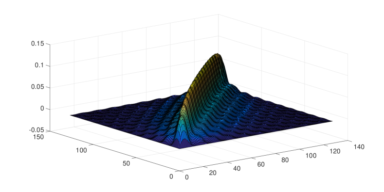
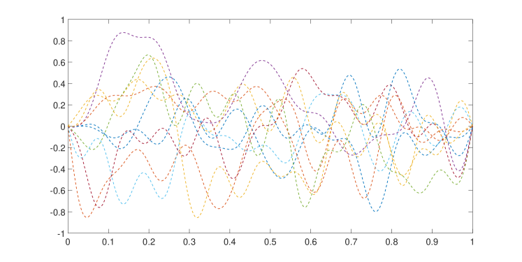
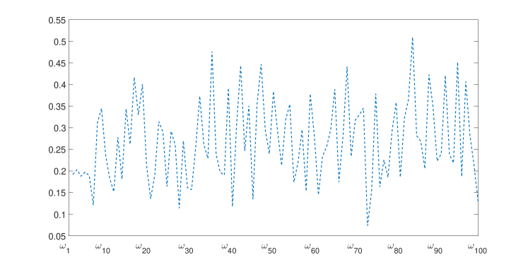
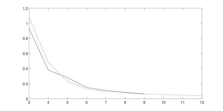
The outline of this paper is as follows. Notation and preliminaries are fixed in Appendix 2. Fundamental assumptions and some key lemmas are formulated in Appendix 3, and proved in Appendix 4. The main result of this paper on strong–consistency is derived in Appendix 5. Appendix 6 provides some examples. Final comments on our approach can be found in Appendix 7. The Supplementary Material provides in Appendix 8 illustrates numerically the results derived in Appendix 5, under the scenario described in Appendix 6, in a simulation study.

2 Preliminaries

Let $\left(B,\left\|\cdot\right\|_{B}\right)$ be a real separable Banach space, with the norm $\left\|\cdot\right\|_{B},$ and let $\mathcal{L}^{2}_{B}(\Omega,\mathcal{A},\mathcal{P}),$ the space of zero-mean $B$–valued random variables $X$ such that

$$\sqrt{\int_{B}\|X\|_{B}^{2}d\mathcal{P}}<\infty.$$

Consider $X=\left\{X_{n},\ n\in\mathbb{Z}\right\}$ to be a zero–mean $B$–valued stochastic process on the basic probability space $\left(\Omega,\mathcal{A},\mathcal{P}\right)$ satisfying (see Bosq [2000]):

$$X_{n}=\rho\left(X_{n-1}\right)+\varepsilon_{n},\quad n\in\mathbb{Z},\quad\rho\in\mathcal{L}(B),$$ (1)

where $\rho$ denotes the autocorrelation operator of $X.$ In equation (1), the $B$–valued innovation process $\varepsilon=\left\{\varepsilon_{n},\ n\in\mathbb{Z}\right\}$ on $\left(\Omega,\mathcal{A},\mathcal{P}\right)$ is assumed to be strong white noise, uncorrelated with the random initial condition. Thus, $\varepsilon$ is a zero–mean Banach–valued stationary process, with independent and identically distributed components, and with $\sigma_{\varepsilon}^{2}={\rm E}\left\{\left\|\varepsilon_{n}\right\|_{B}^{2}\right\}<\infty,$ for each $n\in\mathbb{Z}.$ Assume that there exists an integer $j_{0}\geq 1$ such that

$$\left\|\rho^{j_{0}}\right\|_{\mathcal{L}\left(B\right)}<1.$$ (2)

Then, equation (1) admits an unique strictly stationary solution with $\sigma_{X}^{2}={\rm E}\left\{\left\|X_{n}\right\|_{B}^{2}\right\}<\infty$; i.e., belonging to $\mathcal{L}^{2}_{B}(\Omega,\mathcal{A},\mathcal{P}),$ given by $X_{n}=\displaystyle\sum_{j=0}^{\infty}\rho^{j}\left(\varepsilon_{n-j}\right),$ for each $n\in\mathbb{Z}$ (see Bosq [2000]). Under (2), the autocovariance operator $C$ of an ARB(1) process $X$ is defined from the autocovariance operator of $X_{0}\in\mathcal{L}_{B}^{2}(\Omega,\mathcal{A},\mathcal{P}),$ as

$$C\left(x^{\ast}\right)={\rm E}\left\{x^{\ast}(X_{0})X_{0}\right\},\quad x^{\ast}\in B^{\ast}.$$

The cross–covariance operator $D$ is given by

$$D\left(x^{\ast}\right)={\rm E}\left\{x^{\ast}(X_{0})X_{1}\right\},\quad x^{\ast}\in B^{\ast}.$$

Since $C$ is assumed to be a nuclear operator, there exists a sequence $\left\{x_{j},\ j\geq 1\right\}\subset B$ such that, for every $x^{\ast}\in B^{\ast}$ (see [Bosq, 2000, Eq. (6.24), p. 156]):

$$C(x^{\ast})=\displaystyle\sum_{j=1}^{\infty}x^{\ast}\left(x_{j}\right)x_{j},\quad\displaystyle\sum_{j=1}^{\infty}\left\|x_{j}\right\|_{B}^{2}<\infty.$$

$D$ is also assumed to be a nuclear operator. Then, there exist sequences $\left\{y_{j},\ j\geq 1\right\}\subset B$ and $\left\{x_{j}^{\ast\ast},\ j\geq 1\right\}\subset B^{\ast\ast}$ such that, for every $x^{\ast}\in B^{\ast},$

$$D(x^{\ast})=\displaystyle\sum_{j=1}^{\infty}x_{j}^{\ast\ast}(x^{\ast})y_{j},\quad\displaystyle\sum_{j=1}^{\infty}\left\|x_{j}^{\ast\ast}\right\|_{B^{\ast\ast}}\left\|y_{j}\right\|<\infty,$$

(see [Bosq, 2000, Eq. (6.23), p. 156]). Empirical estimators of $C$ and $D$ are respectively given by (see [Bosq, 2000, Eqs. (6.45) and (6.58), pp. 164–168]), for $n\geq 2,$

$$C_{n}(x^{\ast})=\frac{1}{n}\displaystyle\sum_{i=0}^{n-1}x^{\ast}\left(X_{i}\right)\left(X_{i}\right),\quad D_{n}(x^{\ast})=\frac{1}{n-1}\displaystyle\sum_{i=0}^{n-2}x^{\ast}\left(X_{i}\right)\left(X_{i+1}\right),\quad x^{\ast}\in B^{\ast}.$$

[Kuelbs, 1970, Lemma 2.1], now formulated, plays a key role in our approach.

Lemma 2.1

If $B$ is a real separable Banach space with norm $\left\|\cdot\right\|_{B},$ then, there exists an inner product $\left\langle\cdot,\cdot\right\rangle_{\widetilde{H}}$ on $B$ such that the norm $\left\|\cdot\right\|_{\widetilde{H}},$ generated by $\left\langle\cdot,\cdot\right\rangle_{\widetilde{H}},$ is weaker than $\left\|\cdot\right\|_{B}.$ The completion of $B$ under the norm $\left\|\cdot\right\|_{\widetilde{H}}$ defines the Hilbert space $\widetilde{H},$ where $B$ is continuously embedded.

Denote by $\left\{x_{n},\ n\in\mathbb{N}\right\}\subset B,$ a dense sequence in $B,$ and by $\left\{F_{n},\ n\in\mathbb{N}\right\}\subset B^{\ast}$ a sequence of bounded linear functionals on $B,$ satisfying

$$F_{n}\left(x_{n}\right)=\left\|x_{n}\right\|_{B},\quad\left\|F_{n}\right\|=1,$$ (3)

such that

$$\left\|x\right\|_{B}=\displaystyle\sup_{n\in\mathbb{N}}\left|F_{n}(x)\right|,\quad x\in B.$$ (4)

The inner product $\left\langle\cdot,\cdot\right\rangle_{\widetilde{H}},$ and its associated norm, in Lemma 2.1, is defined by

$$\langle x,y\rangle_{\widetilde{H}} = \displaystyle\sum_{n=1}^{\infty}t_{n}F_{n}(x)F_{n}(y),\quad x,y\in\widetilde{H},$$

$$\left\|x\right\|_{\widetilde{H}}^{2} = \displaystyle\sum_{n=1}^{\infty}t_{n}\left\{F_{n}(x)\right\}^{2}\leq\left\|x\right\|_{B}^{2},\quad x\in B,$$

where $\left\{t_{n},\ n\in\mathbb{N}\right\}$ is a sequence of positive numbers such that $\displaystyle\sum_{n=1}^{\infty}t_{n}=1.$

3 Main assumptions and preliminary results

In view of Lemma 2.1, for every $n\in\mathbb{Z},$ $X_{n}\in B\hookrightarrow\widetilde{H}$ satisfies a.s.

$$X_{n}\underset{\widetilde{H}}{=}\sum_{j=1}^{\infty}\langle X_{n},v_{j}\rangle_{\widetilde{H}}v_{j},\quad n\in\mathbb{Z},$$

for any orthonormal basis $\{v_{j},\ j\geq 1\}$ of $\widetilde{H}.$ The trace autocovariance operator

$$C={\rm E}\left\{\left(\displaystyle\sum_{j=1}^{\infty}\langle X_{n},v_{j}\rangle_{\widetilde{H}}v_{j}\right)\otimes\left(\displaystyle\sum_{j=1}^{\infty}\langle X_{n},v_{j}\rangle_{\widetilde{H}}v_{j}\right)\right\}$$

of the extended ARB(1) process is a trace operator in $\widetilde{H},$ admitting a diagonal spectral representation, in terms of its eigenvalues $\{C_{j},\ j\geq 1\}$ and eigenvectors $\{\phi_{j},\ j\geq 1\},$ that provide an orthonormal system in $\widetilde{H}.$ Summarizing, in the subsequent developments, the following identities in $\widetilde{H}$ will be considered, for the extended version of ARB(1) process $X$. For each $f,h\in\widetilde{H},$

$$C(f)\underset{\widetilde{H}}{=} \sum_{j=1}^{\infty}C_{j}\left\langle f,\phi_{j}\right\rangle_{\widetilde{H}}\phi_{j}$$ (6)

$$D(h)\underset{\widetilde{H}}{=} \sum_{j=1}^{\infty}\sum_{k=1}^{\infty}\left\langle D(\phi_{j}),\phi_{k}\right\rangle_{\widetilde{H}}\left\langle h,\phi_{j}\right\rangle_{\widetilde{H}}\phi_{k}$$

$$C_{n}(f)\underset{\widetilde{H}\ a.s.}{=} \displaystyle\sum_{j=1}^{n}C_{n,j}\left\langle f,\phi_{n,j}\right\rangle_{\widetilde{H}}\phi_{n,j}$$ (7)

$$C_{n,j}\underset{a.s.}{=} \frac{1}{n}\displaystyle\sum_{i=0}^{n-1}X_{i,n,j}^{2},\ X_{i,n,j}=\langle X_{i},\phi_{n,j}\rangle_{\widetilde{H}},\ C_{n}(\phi_{n,j})\underset{\widetilde{H}\ a.s.}{=}C_{n,j}\phi_{n,j}$$

$$D_{n}(h)\underset{\widetilde{H}\ a.s.}{=} \sum_{j=1}^{\infty}\sum_{k=1}^{\infty}\left\langle D_{n}(\phi_{n,j}),\phi_{n,k}\right\rangle_{\widetilde{H}}\left\langle h,\phi_{n,j}\right\rangle_{\widetilde{H}}\phi_{n,k},$$ (8)

where, for $n\geq 2,$ $\left\{\phi_{n,j},\ j\geq 1\right\}$ is a complete orthonormal system in $\widetilde{H},$ and

$$C_{n,1}\geq C_{n,2}\geq\dots\geq C_{n,n}\geq 0=C_{n,n+1}=C_{n,n+2}=\dots.$$

The following assumption plays a crucial role in the derivation of the main results in this paper.

Assumption A1. $\|X_{0}\|_{B}$ is a.s. bounded, and the eigenspace $V_{j},$ associated with $C_{j}>0$ in (6) is one-dimensional for every $j\geq 1.$

Under Assumption A1, we can define the following quantities:

$$a_{1}=2\sqrt{2}\frac{1}{C_{1}-C_{2}},\quad a_{j}=2\sqrt{2}\displaystyle\max\left(\frac{1}{C_{j-1}-C_{j}},\frac{1}{C_{j}-C_{j+1}}\right),\quad j\geq 2.$$ (9)

Remark 3.1

This assumption can be relaxed to considering multidimensional eigenspaces by redefining the quantities $a_{j},$ for each $j\geq 1,$ as the quantities $c_{j},$ for each $j\geq 1,$ given in [Bosq, 2000, Lemma 4.4].

Assumption A2. Let $k_{n}$ such that

$$C_{n,k_{n}}>0,\quad\mbox{(a.s.)}\quad k_{n}\to\infty,\quad\frac{k_{n}}{n}\to 0,\ n\to\infty.$$

Remark 3.2

Consider

$$\Lambda_{k_{n}}=\sup_{1\leq j\leq k_{n}}(C_{j}-C_{j+1})^{-1}.$$ (10)

For $n$ sufficiently large,

$$k_{n}<C_{k_{n}}^{-1}<\frac{1}{C_{k_{n}}-C_{k_{n}+1}}<a_{k_{n}}<\Lambda_{k_{n}}<\displaystyle\sum_{j=1}^{k_{n}}a_{j}.$$

Assumption A3. The following limit holds:

$$\sup_{x\in B;\ \|x\|_{B}\leq 1}\left\|\rho(x)-\sum_{j=1}^{k}\left\langle\rho(x),\phi_{j}\right\rangle_{\widetilde{H}}\phi_{j}\right\|_{B}\to 0,\quad k\to\infty.$$ (11)

Assumption A4. $\left\{C_{j},\ j\geq 1\right\}$ are such that the inclusion of $\mathcal{H}(X)$ into $\widetilde{H}^{\ast}$ is continuous; i.e.,

$$\mathcal{H}(X)\hookrightarrow\widetilde{H}^{\ast},$$

where $\hookrightarrow$ denotes, as usual, the continuous embedding, $\widetilde{H}^{\ast}$ the dual space of $\widetilde{H}$ and $\mathcal{H}(X)$ the Reproducing Kernel Hilbert Space associated with $C$.

Let us consider the closed subspace $H$ of $B$ with the norm induced by the inner product $\left\langle\cdot,\cdot\right\rangle_{H}$ defined as follows:

$$H = \left\{x\in B;\ \sum_{n=1}^{\infty}\left\{F_{n}(x)\right\}^{2}<\infty\right\},\quad\left\langle f,g\right\rangle_{H}=\sum_{n=1}^{\infty}F_{n}(f)F_{n}(g),\quad f,g\in H.$$ (12)

Then, $H$ is continuously embedded into $B,$ and the following remark provides the isometric isomorphism established by the Riesz Representation Theorem between the spaces $\widetilde{H}$ and its dual $\widetilde{H}^{\ast}.$

Remark 3.3

Let $f^{\ast},g^{\ast}\in\widetilde{H}^{\ast},$ and $f,g\in\widetilde{H},$ such that, for every $n\geq 1,$ consider $F_{n}(f^{\ast})=\sqrt{t_{n}}F_{n}(\widetilde{f}),$ $F_{n}(g^{\ast})=\sqrt{t_{n}}F_{n}(\widetilde{g}),$ and $F_{n}(\widetilde{f})=\sqrt{t_{n}}F_{n}(f),$ $F_{n}(\widetilde{g})=\sqrt{t_{n}}F_{n}(g),$ for certain $\widetilde{f},\widetilde{g}\in H.$ Then, the following identities hold:

$$\left\langle f^{\ast},g^{\ast}\right\rangle_{\widetilde{H}^{\ast}} = \sum_{n=1}^{\infty}\frac{1}{t_{n}}F_{n}(f^{\ast})F_{n}(g^{\ast})=\sum_{n=1}^{\infty}\frac{1}{t_{n}}\sqrt{t_{n}}\sqrt{t_{n}}F_{n}(\widetilde{f})F_{n}(\widetilde{g})=\left\langle\widetilde{f},\widetilde{g}\right\rangle_{H}$$

$$= \sum_{n=1}^{\infty}t_{n}F_{n}(f)F_{n}(g)=\left\langle f,g\right\rangle_{\widetilde{H}}.$$

Lemma 3.1

Under Assumption A4, the following continuous embeddings hold:

$$\mathcal{H}(X)\hookrightarrow\widetilde{H}^{\ast}\hookrightarrow B^{\ast}\hookrightarrow H\hookrightarrow B\hookrightarrow\widetilde{H}\hookrightarrow[\mathcal{H}(X)]^{\ast},$$ (13)

where

$$\widetilde{H} = \left\{x\in B;\ \sum_{n=1}^{\infty}t_{n}\left\{F_{n}(x)\right\}^{2}<\infty\right\},\quad\left\langle f,g\right\rangle_{\widetilde{H}}=\sum_{n=1}^{\infty}t_{n}F_{n}(f)F_{n}(g),\ f,g\in\widetilde{H}$$

$$H = \left\{x\in B;\ \sum_{n=1}^{\infty}\left\{F_{n}(x)\right\}^{2}<\infty\right\},\quad\left\langle f,g\right\rangle_{H}=\sum_{n=1}^{\infty}F_{n}(f)F_{n}(g),\ f,g\in H$$

$$\widetilde{H}^{\ast} = \left\{x\in B;\ \sum_{n=1}^{\infty}\frac{1}{t_{n}}\left\{F_{n}(x)\right\}^{2}<\infty\right\},\quad\left\langle f,g\right\rangle_{\widetilde{H}^{\ast}}=\sum_{n=1}^{\infty}\frac{1}{t_{n}}F_{n}(f)F_{n}(g),\ f,g\in\widetilde{H}^{\ast}$$

$$\mathcal{H}(X) = \left\{x\in\widetilde{H};\ \left\langle C^{-1}(x),x\right\rangle_{\widetilde{H}}<\infty\right\},$$

$$\left\langle f,g\right\rangle_{\mathcal{H}(X)} = \left\langle C^{-1}(f),g\right\rangle_{\widetilde{H}},\ f,g\in C^{1/2}(\widetilde{H})$$

$$\left[\mathcal{H}(X)\right]^{\ast} = \left\{x\in\widetilde{H};\ \left\langle C(x),x\right\rangle_{\widetilde{H}}<\infty\right\}$$

$$\left\langle f,g\right\rangle_{[\mathcal{H}(X)]^{\ast}} = \left\langle C(f),g\right\rangle_{\widetilde{H}}\ f,g\in C^{-1/2}(\widetilde{H}).$$

Proof. Let us consider the following inequalitites, for each $x\in B$,:

$$\|x\|_{\widetilde{H}} = \sqrt{\sum_{j=1}^{\infty}t_{n}\left\{F_{n}(x)\right\}^{2}}\leq\|x\|_{B}=\sup_{n\geq 1}|F_{n}(x)|,$$

$$\|x\|_{B} = \sup_{n\geq 1}|F_{n}(x)|\leq\sqrt{\sum_{n=1}^{\infty}\left\{F_{n}(x)\right\}^{2}}=\|x\|_{H}\leq\sum_{n=1}^{\infty}|F_{n}(x)|=\|x\|_{B^{\ast}},$$

$$\|x\|_{B^{\ast}} = \sum_{n=1}^{\infty}|F_{n}(x)|\leq\sqrt{\sum_{n=1}^{\infty}\frac{1}{t_{n}}\left\{F_{n}(x)\right\}^{2}}=\|x\|_{\widetilde{H}^{\ast}}.$$ (14)

Under Assumption A4 (see also Remark 3.3), for every $f\in C^{1/2}(\widetilde{H})=\mathcal{H}(X),$

$$\|f\|_{\mathcal{H}(X)}=\sqrt{\left\langle C^{-1}(f),f\right\rangle_{\widetilde{H}}}\geq\|f\|_{\widetilde{H}^{\ast}}=\sqrt{\sum_{n=1}^{\infty}\frac{1}{t_{n}}\left\{F_{n}(x)\right\}^{2}}.$$ (15)

From equations (14)–(15), the inclusions in (13) are continuous.

$\blacksquare$

It is well–known that $\{\phi_{j},\ j\geq 1\}$ is also an orthogonal system in $\mathcal{H}(X).$ Futhermore, under Assumption A4, from Lemma 3.1,

$$\{\phi_{j},\ j\geq 1\}\subset\mathcal{H}(X)\hookrightarrow\widetilde{H}^{\ast}\hookrightarrow B^{\ast}\hookrightarrow H.$$

Therefore, from equation (12), for every $j\geq 1,$

$$\|\phi_{j}\|_{H}^{2}=\sum_{m=1}^{\infty}\left\{F_{m}(\phi_{j})\right\}^{2}<\infty.$$ (16)

The following assumption is now considered on the norm (16):

Assumption A5. The continuous embedding $i_{\mathcal{H}(X),H}:\mathcal{H}(X)\hookrightarrow H$ belongs to the trace class. That is,

$$\sum_{j=1}^{\infty}\|\phi_{j}\|_{H}^{2}<\infty.$$

Let $\{F_{m},\ m\geq 1\}$ be defined as in Lemma 2.1. Assumption A5 leads to

$$\sum_{j=1}^{\infty}\left\langle i_{\mathcal{H}(X),H}(\phi_{j}),\phi_{j}\right\rangle_{H}=\sum_{j=1}^{\infty}\sum_{m=1}^{\infty}\left\{F_{m}(\phi_{j})\right\}^{2}=\sum_{m=1}^{\infty}N_{m}<\infty,$$ (17)

where, in particular, from equation (17),

$$N_{m} = \sum_{j=1}^{\infty}\left\{F_{m}(\phi_{j})\right\}^{2}<\infty,\quad\sup_{m\geq 1}N_{m}=N<\infty$$ (18)

$$V = \displaystyle\sup_{j\geq 1}\left\|\phi_{j}\right\|_{B}\leq\sum_{j=1}^{\infty}\sum_{m=1}^{\infty}\left\{F_{m}(\phi_{j})\right\}^{2}<\infty.$$ (19)

The following preliminary results are considered from [Bosq, 2000, Theorem 4.1, pp. 98–99; Corollary 4.1, pp. 100–101; Theorem 4.8, pp. 116–117]).

Lemma 3.2

Under Assumption A1, the following identities hold, for any standard AR$\widetilde{H}$(1) process (e.g., the extension to $\widetilde{H}$ of ARB(1) process $X$ satisfying equation (1)),

$$\left\|C_{n}-C\right\|_{\mathcal{S}(\widetilde{H})}=\mathcal{O}\left(\left(\frac{\ln(n)}{n}\right)^{1/2}\right)\leavevmode\nobreak\ a.s.,\quad\left\|D_{n}-D\right\|_{\mathcal{S}(\widetilde{H})}=\mathcal{O}\left(\left(\frac{\ln(n)}{n}\right)^{1/2}\right)\leavevmode\nobreak\ a.s.,$$

(20)

where $\left\|\cdot\right\|_{\mathcal{S}(\widetilde{H})}$ is the norm in the Hilbert space $\mathcal{S}(\widetilde{H})$ of Hilbert–Schmidt operators on $\widetilde{H}$; i.e., the subspace of compact operators $\mathcal{A}$ such that

$$\sum_{j=1}^{\infty}\left\langle\mathcal{A}^{\ast}\mathcal{A}(\varphi_{j}),\varphi_{j}\right\rangle_{\widetilde{H}}<\infty,$$

for any orthonormal basis $\{\varphi_{j},\ j\geq 1\}$ of $\widetilde{H}.$

Lemma 3.3

Under Assumption A1, let $\{C_{j},\ j\geq 1\}$ and $\{C_{n,j},\ j\geq 1\}$ in (6)– (7), respectively. Then,

$$\left(\frac{n}{\ln(n)}\right)^{1/2}\sup_{j\geq 1}\left|C_{n,j}-C_{j}\right|\longrightarrow 0\leavevmode\nobreak\ a.s.,\quad n\to\infty.$$

Lemma 3.4

(See details in [Bosq, 2000, Corollary 4.3, p. 107]) Under Assumption A1, consider $\Lambda_{k_{n}}$ in equation (10) satisfying

$$\Lambda_{k_{n}}=o\left(\left(\frac{n}{\ln(n)}\right)^{1/2}\right),\quad n\rightarrow\infty.$$

Then,

$$\sup_{1\leq j\leq k_{n}}\|\phi_{n,j}^{\prime}-\phi_{n,j}\|_{\widetilde{H}}\longrightarrow 0\leavevmode\nobreak\ a.s.,\quad n\rightarrow\infty,$$

where, for $j\geq 1,$ and $n\geq 2,$

$$\phi_{n,j}^{\prime}={\rm sgn}\langle\phi_{n,j},\phi_{j}\rangle_{\widetilde{H}}\phi_{j},\quad{\rm sgn}\langle\phi_{n,j},\phi_{j}\rangle_{\widetilde{H}}=\boldsymbol{1}_{\langle\phi_{n,j},\phi_{j}\rangle_{\widetilde{H}}\geq 0}-\boldsymbol{1}_{\langle\phi_{n,j},\phi_{j}\rangle_{\widetilde{H}}<0},$$

with $\boldsymbol{1}_{\cdot}$ being the indicator function.

An upper bound for $\left\|c\right\|_{B\times B}=\left\|\displaystyle\sum_{j=1}^{\infty}C_{j}\phi_{j}\otimes\phi_{j}\right\|_{B\times B}$ is now obtained.

Lemma 3.5

Under Assumption A5, the following inequality holds:

$$\left\|c\right\|_{B\times B}=\sup_{n,m\geq 1}\left|C\left(F_{n}\right)\left(F_{m}\right)\right|\leq N\left\|C\right\|_{\mathcal{L}(\widetilde{H})},$$

where $N$ has been introduced in equation (18), $\mathcal{L}(\widetilde{H})$ denotes the space of bounded linear operators on $\widetilde{H},$ and $\left\|\cdot\right\|_{\mathcal{L}(\widetilde{H})}$ the usual uniform norm on such a space.

Let us consider the following notation.

$$c\underset{\widetilde{H}\otimes\widetilde{H}}{=} \sum_{j=1}^{\infty}C_{j}\phi_{n,j}^{\prime}\otimes\phi_{n,j}^{\prime}\underset{\widetilde{H}\otimes\widetilde{H}}{=}\sum_{j=1}^{\infty}C_{j}\phi_{j}\otimes\phi_{j},\quad c_{n}\underset{\widetilde{H}\otimes\widetilde{H}}{=}\sum_{j=1}^{\infty}C_{n,j}\phi_{n,j}\otimes\phi_{n,j}.$$

$$c-c_{n}\underset{\widetilde{H}\otimes\widetilde{H}}{=} \sum_{j=1}^{\infty}C_{j}\phi^{\prime}_{n,j}\otimes\phi^{\prime}_{n,j}-\sum_{j=1}^{\infty}C_{n,j}\phi_{n,j}\otimes\phi_{n,j}$$ (21)

Remark 3.4

From Lemma 3.2, for $n$ sufficiently large, there exist positive constants $K_{1}$ and $K_{2}$ such that

$$K_{1}\left\langle C(\varphi),\varphi\right\rangle_{\widetilde{H}}\leq\left\langle C_{n}(\varphi),\varphi\right\rangle_{\widetilde{H}}\leq K_{2}\left\langle C(\varphi),\varphi\right\rangle_{\widetilde{H}},\quad\forall\varphi\in\widetilde{H}.$$

In particular, for every $x\in\mathcal{H}(X)=C^{1/2}(\widetilde{H}),$ considering $n$ sufficiently large,

$$\frac{1}{K_{1}}\left\langle C^{-1}(x),x\right\rangle_{\widetilde{H}}\geq\left\langle C_{n}^{-1}(x),x\right\rangle_{\widetilde{H}}\geq\frac{1}{K_{2}}\left\langle C^{-1}(x),x\right\rangle_{\widetilde{H}}$$

$$\Leftrightarrow\ \frac{1}{K_{1}}\|x\|_{\mathcal{H}(X)}^{2}\geq\left\langle C_{n}^{-1}(x),x\right\rangle_{\widetilde{H}}\geq\frac{1}{K_{2}}\|x\|_{\mathcal{H}(X)}^{2}.$$ (22)

Equation (22) means that, for $n$ sufficiently large, the norm of the RKHS $\mathcal{H}(X)$ of $X$ is equivalent to the norm of the RKHS generated by $C_{n},$ with spectral kernel $c_{n}$ given in (21).

Lemma 3.6

Under Assumptions A1 and A4–A5, let us consider $\Lambda_{k_{n}}$ in (10) satisfying

$$\sqrt{k_{n}}\Lambda_{k_{n}}=o\left(\sqrt{\frac{n}{\ln(n)}}\right),\quad n\to\infty,$$ (23)

where $k_{n}$ has been introduced in Assumption A2. The following a.s. inequality then holds:

$$\left\|c-c_{n}\right\|_{B\times B}\leq\max(N,\sqrt{N})\left[\|C-C_{n}\|_{\mathcal{L}(\widetilde{H})}\right.$$

$$\left.+2\max\left(\sqrt{\|C\|_{\mathcal{L}(\widetilde{H})}},\sqrt{\|C_{n}\|_{\mathcal{L}(\widetilde{H})}}\right)\left[\sup_{l\geq 1}\sup_{m\geq 1}\left|F_{l}(\phi^{\prime}_{n,m})\right|\right]\right.$$

$$\times\sqrt{k_{n}8\Lambda_{k_{n}}^{2}\|C_{n}-C\|_{\mathcal{L}(\widetilde{H})}^{2}+\sum_{m=k_{n}+1}^{\infty}\|\phi_{n,m}-\phi_{n,m}^{\prime}\|_{\widetilde{H}}^{2}}.$$

Therefore, $\left\|c-c_{n}\right\|_{B\times B}\to_{a.s.}0,$ as $n\to\infty.$

Lemma 3.7

For a standard ARB(1) process satisfying equation (1), under Assumptions A1 and A3–A5, for $n$ sufficiently large,

$$\sup_{1\leq j\leq k_{n}}\left\|\phi_{n,j}-\phi_{n,j}^{\prime}\right\|_{B}$$

$$\leq\frac{2}{C_{k_{n}}}\left[\max(N,\sqrt{N})\left[\|C-C_{n}\|_{\mathcal{L}(\widetilde{H})}\right.\right.$$

$$\left.\left.+2\max\left(\sqrt{\|C\|_{\mathcal{L}(\widetilde{H})}},\sqrt{\|C_{n}\|_{\mathcal{L}(\widetilde{H})}}\right)\left(\sup_{l\geq 1}\sup_{m\geq 1}\left|F_{l}(\phi^{\prime}_{n,m})\right|\right)\right.\right.$$

$$\left.\left.\times\sqrt{k_{n}8\Lambda_{k_{n}}^{2}\|C_{n}-C\|_{\mathcal{L}(\widetilde{H})}^{2}+\sum_{m=k_{n}+1}^{\infty}\|\phi_{n,m}-\phi_{n,m}^{\prime}\|_{\widetilde{H}}^{2}}\right]\right.$$

$$\left.+\sup_{1\leq j\leq k_{n}}\|\phi_{n,j}-\phi_{n,j}^{\prime}\|_{\widetilde{H}}N\|C\|_{\mathcal{S}(\widetilde{H})}+V\|C-C_{n}\|_{\mathcal{S}(\widetilde{H})}\right]\quad\mbox{a.s.}$$ (24)

Under (23),

$$\sup_{1\leq j\leq k_{n}}\left\|\phi_{n,j}-\phi_{n,j}^{\prime}\right\|_{B}\longrightarrow 0\leavevmode\nobreak\ a.s.,\quad n\to\infty.$$

Lemma 3.8

Under Assumption A3, if

$$\sum_{j=1}^{k_{n}}\|\phi_{n,j}-\phi_{n,j}^{\prime}\|_{B}\to_{a.s.}0,,\quad n\to\infty,$$

then

$$\sup_{x\in B;\ \|x\|_{B}\leq 1}\left\|\rho(x)-\sum_{j=1}^{k_{n}}\left\langle\rho(x),\phi_{n,j}\right\rangle_{\widetilde{H}}\phi_{n,j}\right\|_{B}\longrightarrow 0\leavevmode\nobreak\ a.s.,\quad n\to\infty.$$ (25)

Remark 3.5

Under the conditions of Lemma 3.7, if

$$k_{n}^{3/2}\Lambda_{k_{n}}=o\left(\sqrt{\frac{n}{\ln(n)}}\right),\quad\sum_{m=k_{n}+1}^{\infty}\|\phi_{n,m}-\phi_{n,m}^{\prime}\|_{\widetilde{H}}^{2}=o\left(\frac{1}{k_{n}}\right),\ n\to\infty,$$

then, equation (25) holds.

Let us know consider the projection operators

$$\widetilde{\Pi}^{k_{n}}\left(x\right) = \displaystyle\sum_{j=1}^{k_{n}}\langle x,\phi_{n,j}\rangle_{\widetilde{H}}\phi_{n,j},\quad\Pi^{k_{n}}\left(x\right)=\displaystyle\sum_{j=1}^{k_{n}}\langle x,\phi_{n,j}^{\prime}\rangle_{\widetilde{H}}\phi_{n,j}^{\prime},\quad x\in B\subset\widetilde{H}.$$ (26)

Remark 3.6

Under the conditions of Remark 3.5, let

$$\widetilde{\Pi}^{k_{n}}\rho\widetilde{\Pi}^{k_{n}}=\sum_{j=1}^{k_{n}}\sum_{p=1}^{k_{n}}\left\langle\rho(\phi_{n,j}),\phi_{n,p}\right\rangle_{\widetilde{H}}\phi_{n,j}\otimes\phi_{n,p},$$

then

$$\sup_{x\in B;\ \|x\|_{B}\leq 1}\left\|\rho(x)-\sum_{j=1}^{k_{n}}\sum_{p=1}^{k_{n}}\left\langle x,\phi_{n,j}\right\rangle_{\widetilde{H}}\left\langle\rho(\phi_{n,j}),\phi_{n,p}\right\rangle_{\widetilde{H}}\phi_{n,p}\right\|_{B}\longrightarrow 0\leavevmode\nobreak\ a.s.,\ n\to\infty.$$

4 Proofs of Lemmas

Proof of Lemma 3.5

Proof. Applying the Cauchy–Schwarz’s inequality, for every $k,l\geq 1,$

$$|C(F_{k},F_{l})| = \left|\sum_{j=1}^{\infty}C_{j}F_{k}(\phi_{j})F_{l}(\phi_{j})\right|\leq\sqrt{\sum_{j=1}^{\infty}C_{j}[F_{k}(\phi_{j})]^{2}\sum_{p=1}^{\infty}C_{p}[F_{l}(\phi_{p})]^{2}}$$

$$\leq \sup_{j\geq 1}|C_{j}|\sqrt{\sum_{j=1}^{\infty}[F_{k}(\phi_{j})]^{2}\sum_{p=1}^{\infty}[F_{l}(\phi_{p})]^{2}}=\sup_{j\geq 1}|C_{j}|\sqrt{N_{k}N_{l}},$$

where $\{F_{n},\ n\geq 1\}$ have been introduced in equation (3), and satisfy (4)–(LABEL:A7:ineq_norm). Under Assumption A5, from equation (18),

$$\|c\|_{B\times B}=\sup_{k,l\geq 1}|C(F_{k},F_{l})|\leq\sup_{k,l\geq 1}\sup_{j\geq 1}|C_{j}|\sqrt{N_{k}N_{l}}=N\sup_{j\geq 1}|C_{j}|=N\|C\|_{\mathcal{L}(\widetilde{H})}.$$

$\blacksquare$

Proof of Lemma 3.6

Proof. Let us first consider the following identities and inequalities:

$$|C-C_{n}(F_{k})(F_{l})| = \left|\sum_{j=1}^{\infty}C_{j}F_{k}(\phi_{n,j}^{\prime})F_{l}(\phi_{n,j}^{\prime})-C_{n,j}F_{k}(\phi_{n,j})F_{l}(\phi_{n,j})\right|$$

$$\leq \sum_{j=1}^{\infty}|C_{j}||F_{k}(\phi_{n,j}^{\prime})||F_{l}(\phi_{n,j}^{\prime})-F_{l}(\phi_{n,j})|$$

$$\hskip 28.45274pt+\sup_{j}|C_{j}-C_{n,j}||F_{k}(\phi_{n,j}^{\prime})F_{l}(\phi_{n,j})|$$

$$\hskip 28.45274pt+|C_{n,j}F_{l}(\phi_{n,j})||F_{k}(\phi_{n,j}^{\prime})-F_{k}(\phi_{n,j})|$$

$$\leq \sqrt{\sum_{j=1}^{\infty}C_{j}\left\{F_{k}(\phi_{n,j}^{\prime})\right\}^{2}\sum_{j=1}^{\infty}C_{j}\left\{F_{l}(\phi_{n,j}^{\prime})-F_{l}(\phi_{n,j})\right\}^{2}}$$

$$+ \sup_{j\geq 1}|C_{j}-C_{n,j}|\sqrt{\sum_{j=1}^{\infty}\left\{F_{k}(\phi_{n,j}^{\prime})\right\}^{2}\sum_{j=1}^{\infty}\left\{F_{l}(\phi_{n,j})\right\}^{2}}$$

$$+ \sqrt{\sum_{j=1}^{\infty}C_{n,j}\left\{F_{l}(\phi_{n,j})\right\}^{2}\sum_{j=1}^{\infty}C_{n,j}\left\{F_{k}(\phi_{n,j}^{\prime})-F_{k}(\phi_{n,j})\right\}^{2}}$$

$$\leq \sqrt{N_{k}}\sqrt{\sum_{j=1}^{\infty}C_{j}\left\{F_{l}(\phi_{n,j}^{\prime})-F_{l}(\phi_{n,j})\right\}^{2}}$$

$$+ \sup_{j\geq 1}|C_{j}-C_{n,j}|\sqrt{N_{k}}\sqrt{N_{l}}$$

$$+ \sqrt{N_{l}}\sqrt{\sum_{j=1}^{\infty}C_{n,j}\left\{F_{k}(\phi_{n,j}^{\prime})-F_{k}(\phi_{n,j})\right\}^{2}}$$

$$\leq \max(N,\sqrt{N})\left[\sqrt{\|C\|_{\mathcal{L}(\widetilde{H})}\sum_{j=1}^{\infty}\left\{F_{l}(\phi_{n,j}^{\prime}-\phi_{n,j})\right\}^{2}}\right.$$

$$\left.+\|C-C_{n}\|_{\mathcal{L}(\widetilde{H})}\right.$$

$$\left.+\sqrt{\|C_{n}\|_{\mathcal{L}(\widetilde{H})}\sum_{j=1}^{\infty}\left\{F_{k}(\phi_{n,j}^{\prime}-\phi_{n,j})\right\}^{2}}\right]$$

$$\leq \max(N,\sqrt{N})\left[\|C-C_{n}\|_{\mathcal{L}(\widetilde{H})}\right.$$

$$\left.+\sqrt{\|C\|_{\mathcal{L}(\widetilde{H})}\sum_{j=1}^{\infty}\sum_{m=1}^{\infty}\left\{F_{l}(\phi^{\prime}_{n,m})\right\}^{2}\left\{\left\langle\phi_{n,j}^{\prime},\phi_{n,m}^{\prime}\right\rangle_{\widetilde{H}}-\left\langle\phi_{n,j},\phi_{n,m}^{\prime}\right\rangle_{\widetilde{H}}\right\}^{2}}\right.$$

$$\left.+\sqrt{\|C_{n}\|_{\mathcal{L}(\widetilde{H})}\sum_{j=1}^{\infty}\sum_{m=1}^{\infty}\left\{F_{k}(\phi^{\prime}_{n,m})\right\}^{2}\left\{\left\langle\phi_{n,j}^{\prime},\phi_{n,m}^{\prime}\right\rangle_{\widetilde{H}}-\left\langle\phi_{n,j},\phi_{n,m}^{\prime}\right\rangle_{\widetilde{H}}\right\}^{2}}\right]$$

$$= \max(N,\sqrt{N})\left[\|C-C_{n}\|_{\mathcal{L}(\widetilde{H})}\right.$$

$$\left.+\sqrt{\|C\|_{\mathcal{L}(\widetilde{H})}\sum_{m=1}^{\infty}\left\{F_{l}(\phi^{\prime}_{n,m})\right\}^{2}\sum_{j=1}^{\infty}\left\{\left\langle\phi_{n,j}^{\prime},\phi_{n,m}^{\prime}\right\rangle_{\widetilde{H}}-\left\langle\phi_{n,j},\phi_{n,m}^{\prime}\right\rangle_{\widetilde{H}}\right\}^{2}}\right.$$

$$\left.+\sqrt{\|C_{n}\|_{\mathcal{L}(\widetilde{H})}\sum_{m=1}^{\infty}\left\{F_{k}(\phi^{\prime}_{n,m})\right\}^{2}\sum_{j=1}^{\infty}\left\{\left\langle\phi_{n,j}^{\prime},\phi_{n,m}^{\prime}\right\rangle_{\widetilde{H}}-\left\langle\phi_{n,j},\phi_{n,m}^{\prime}\right\rangle_{\widetilde{H}}\right\}^{2}}\right]$$

$$= \max(N,\sqrt{N})\left[\|C-C_{n}\|_{\mathcal{L}(\widetilde{H})}\right.$$

$$\left.+\sqrt{\|C\|_{\mathcal{L}(\widetilde{H})}\sum_{m=1}^{\infty}\left\{F_{l}(\phi^{\prime}_{n,m})\right\}^{2}\sum_{j=1}^{\infty}\left\{\left\langle\phi_{n,j},\phi_{n,m}\right\rangle_{\widetilde{H}}-\left\langle\phi_{n,j},\phi_{n,m}^{\prime}\right\rangle_{\widetilde{H}}\right\}^{2}}\right.$$

$$\left.+\sqrt{\|C_{n}\|_{\mathcal{L}(\widetilde{H})}\sum_{m=1}^{\infty}\left\{F_{k}(\phi^{\prime}_{n,m})\right\}^{2}\sum_{j=1}^{\infty}\left\{\left\langle\phi_{n,j},\phi_{n,m}\right\rangle_{\widetilde{H}}-\left\langle\phi_{n,j},\phi_{n,m}^{\prime}\right\rangle_{\widetilde{H}}\right\}^{2}}\right]$$

$$= \max(N,\sqrt{N})\left[\|C-C_{n}\|_{\mathcal{L}(\widetilde{H})}\right.$$

$$\left.+\sqrt{\|C\|_{\mathcal{L}(\widetilde{H})}\sum_{m=1}^{\infty}\left\{F_{l}(\phi^{\prime}_{n,m})\right\}^{2}\|\phi_{n,m}-\phi_{n,m}^{\prime}\|_{\widetilde{H}}^{2}}\right.$$

$$\left.+\sqrt{\|C_{n}\|_{\mathcal{L}(\widetilde{H})}\sum_{m=1}^{\infty}\left\{F_{k}(\phi^{\prime}_{n,m})\right\}^{2}\|\phi_{n,m}-\phi_{n,m}^{\prime}\|_{\widetilde{H}}^{2}}\right]$$

$$\leq \max(N,\sqrt{N})\left[\|C-C_{n}\|_{\mathcal{L}(\widetilde{H})}\right.$$

$$\left.+\sup_{m\geq 1}\left|F_{l}(\phi^{\prime}_{n,m})\right|\sqrt{\|C\|_{\mathcal{L}(\widetilde{H})}\sum_{m=1}^{\infty}\|\phi_{n,m}-\phi_{n,m}^{\prime}\|_{\widetilde{H}}^{2}}\right.$$

$$\left.+\sup_{m\geq 1}\left|F_{k}(\phi^{\prime}_{n,m})\right|\sqrt{\|C_{n}\|_{\mathcal{L}(\widetilde{H})}\sum_{m=1}^{\infty}\|\phi_{n,m}-\phi_{n,m}^{\prime}\|_{\widetilde{H}}^{2}}\right]$$

$$\leq \max(N,\sqrt{N})\left[\|C-C_{n}\|_{\mathcal{L}(\widetilde{H})}\right.$$ (27)

$$\left.+\max\left(\sqrt{\|C\|_{\mathcal{L}(\widetilde{H})}},\sqrt{\|C_{n}\|_{\mathcal{L}(\widetilde{H})}}\right)\right.$$

$$\left.\left[\sup_{m\geq 1}\left|F_{l}(\phi^{\prime}_{n,m})\right|+\sup_{m\geq 1}\left|F_{k}(\phi^{\prime}_{n,m})\right|\right]\sqrt{\sum_{m=1}^{\infty}\|\phi_{n,m}-\phi_{n,m}^{\prime}\|_{\widetilde{H}}^{2}}\right].$$

Under Assumption A5, from equation (17),

$$\sum_{m=1}^{\infty}\|\phi_{n,m}-\phi_{n,m}^{\prime}\|_{\widetilde{H}}^{2}<\infty,\quad\sup_{m\geq 1}\left|F_{k}(\phi^{\prime}_{n,m})\right|<\infty,\quad k\geq 1.$$

Thus, considering $k_{n},$ as given in Assumption A2,

$$\sum_{m=1}^{\infty}\|\phi_{n,m}-\phi_{n,m}^{\prime}\|_{\widetilde{H}}^{2}=\sum_{m=1}^{k_{n}}\|\phi_{n,m}-\phi_{n,m}^{\prime}\|_{\widetilde{H}}^{2}+\sum_{m=k_{n}+1}^{\infty}\|\phi_{n,m}-\phi_{n,m}^{\prime}\|_{\widetilde{H}}^{2}$$

$$\leq k_{n}\sup_{1\leq m\leq k_{n}}\|\phi_{n,m}-\phi_{n,m}^{\prime}\|_{\widetilde{H}}^{2}+\sum_{m=k_{n}+1}^{\infty}\|\phi_{n,m}-\phi_{n,m}^{\prime}\|_{\widetilde{H}}^{2}$$

$$\leq k_{n}8\Lambda_{k_{n}}^{2}\|C_{n}-C\|_{\mathcal{L}(\widetilde{H})}^{2}+\sum_{m=k_{n}+1}^{\infty}\|\phi_{n,m}-\phi_{n,m}^{\prime}\|_{\widetilde{H}}^{2}$$ (28)

From equation (20), under $\Lambda_{k_{n}}=o\left(\sqrt{\frac{n}{\ln(n)}}\right),$

$$k_{n}8\Lambda_{k_{n}}^{2}\|C_{n}-C\|_{\mathcal{L}(\widetilde{H})}^{2}\leq k_{n}8\Lambda_{k_{n}}^{2}\|C_{n}-C\|_{\mathcal{S}(\widetilde{H})}^{2}\to_{a.s.}0,\ n\to\infty.$$ (29)

Under Assumption A5,

$$\sum_{m=k_{n}+1}^{\infty}\|\phi_{n,m}-\phi_{n,m}^{\prime}\|_{\widetilde{H}}^{2}\to_{a.s.}0,\quad n\to\infty.$$ (30)

From equations (27)–(30), since, under Assumption A5,

$$\sup_{k\geq 1}\sup_{m\geq 1}\left|F_{k}(\phi^{\prime}_{n,m})\right|<\infty,$$

we have $\|c-c_{n}\|_{B\times B}=\sup_{k,l}|(C-C_{n})(F_{k})(F_{l})|\to_{a.s.}0,$ as $n\to\infty.$

$\blacksquare$

Proof of Lemma 3.7

Proof. Let us first consider the following a.s. equalities

$$C_{n,j}\left(\phi_{n,j}-\phi_{n,j}^{\prime}\right) = C_{n}\left(\phi_{n,j}\right)-C_{n,j}\phi_{n,j}^{\prime}=\left(C_{n}-C\right)\left(\phi_{n,j}\right)$$ (31)

$$+ C\left(\phi_{n,j}-\phi_{n,j}^{\prime}\right)+\left(C_{j}-C_{n,j}\right)\phi_{n,j}^{\prime}.$$

From equation (31), keeping in mind Assumption A2,

$$\left\|\phi_{n,j}-\phi_{n,j}^{\prime}\right\|_{B} \leq \frac{1}{C_{n,j}}\left\|\left(C_{n}-C\right)\left(\phi_{n,j}\right)\right\|_{B}+\frac{1}{C_{n,j}}\left\|C\left(\phi_{n,j}-\phi_{n,j}^{\prime}\right)\right\|_{B}$$ (32)

$$+ \frac{1}{C_{n,j}}\left\|\left(C_{j}-C_{n,j}\right)\phi_{n,j}^{\prime}\right\|_{B}=\frac{1}{C_{n,j}}\left[S_{1}+S_{2}+S_{3}\right],\quad\mbox{a.s.}.$$

For $n$ sufficiently large, from Lemmas 3.5 and 3.6, applying the Cauchy–Schwarz’s inequality, for every $j\geq 1,$

$$S_{1} = \left\|\left(C_{n}-C\right)\left(\phi_{n,j}\right)\right\|_{B}$$

$$= \sup_{m}\left|\sum_{k=1}^{\infty}C_{n,k}F_{m}(\phi_{n,k})\left\langle\phi_{n,k},\phi_{n,j}\right\rangle_{\widetilde{H}}-\sum_{k=1}^{\infty}C_{k}F_{m}(\phi_{n,k}^{\prime})\left\langle\phi_{n,k}^{\prime},\phi_{n,j}\right\rangle_{\widetilde{H}}\right|$$

$$= \sup_{m}\left|\sum_{k=1}^{\infty}\sum_{l=1}^{\infty}t_{l}F_{l}(\phi_{n,j})\left\{C_{n,k}F_{m}(\phi_{n,k})F_{l}(\phi_{n,k})-C_{k}F_{m}(\phi_{n,k}^{\prime})F_{l}(\phi_{n,k}^{\prime})\right\}\right|$$

$$= \sup_{m}\left|\sum_{l=1}^{\infty}t_{l}F_{l}(\phi_{n,j})\sum_{k=1}^{\infty}C_{n,k}F_{m}(\phi_{n,k})F_{l}(\phi_{n,k})-C_{k}F_{m}(\phi_{n,k}^{\prime})F_{l}(\phi_{n,k}^{\prime})\right|$$

$$\leq \sup_{m}\sqrt{\sum_{l=1}^{\infty}t_{l}[F_{l}(\phi_{n,j})]^{2}}$$

$$\hskip 28.45274pt\times\sqrt{\sum_{l=1}^{\infty}t_{l}\left\{\sum_{k=1}^{\infty}C_{n,k}F_{m}(\phi_{n,k})F_{l}(\phi_{n,k})-C_{k}F_{m}(\phi_{n,k}^{\prime})F_{l}(\phi_{n,k}^{\prime})\right\}^{2}}$$

$$\leq \|\phi_{n,j}\|_{\widetilde{H}}\sqrt{\sum_{l=1}^{\infty}t_{l}}\sup_{m,l}\left|\sum_{k=1}^{\infty}C_{n,k}F_{m}(\phi_{n,k})F_{l}(\phi_{n,k})-C_{k}F_{m}(\phi_{n,k}^{\prime})F_{l}(\phi_{n,k}^{\prime})\right|$$

$$=\|c_{n}-c\|_{B\times B}$$

$$\leq\max(N,\sqrt{N})\left[\|C-C_{n}\|_{\mathcal{L}(\widetilde{H})}\right.$$

$$\left.+2\max\left(\sqrt{\|C\|_{\mathcal{L}(\widetilde{H})}},\sqrt{\|C_{n}\|_{\mathcal{L}(\widetilde{H})}}\right)\left[\sup_{l\geq 1}\sup_{m\geq 1}\left|F_{l}(\phi^{\prime}_{n,m})\right|\right]\right.$$

$$\times\sqrt{k_{n}8\Lambda_{k_{n}}^{2}\|C_{n}-C\|_{\mathcal{L}(\widetilde{H})}^{2}+\sum_{m=k_{n}+1}^{\infty}\|\phi_{n,m}-\phi_{n,m}^{\prime}\|_{\widetilde{H}}^{2}}$$ (33)

$$S_{2} = \left\|C\left(\phi_{n,j}-\phi_{n,j}^{\prime}\right)\right\|_{B}=\sup_{m}\left|\sum_{k=1}^{\infty}\sum_{l=1}^{\infty}t_{l}C_{k}F_{m}(\phi_{n,k}^{\prime})F_{l}(\phi_{n,k}^{\prime})F_{l}\left(\phi_{n,j}-\phi_{n,j}^{\prime}\right)\right|$$

$$\leq \sup_{m}\sqrt{\sum_{l=1}^{\infty}t_{l}\left\{F_{l}\left(\phi_{n,j}-\phi_{n,j}^{\prime}\right)\right\}^{2}}\sqrt{\sum_{l=1}^{\infty}t_{l}\left\{\sum_{k=1}^{\infty}C_{k}F_{m}(\phi_{n,k}^{\prime})F_{l}(\phi_{n,k}^{\prime})\right\}^{2}}$$

$$\leq \|\phi_{n,j}-\phi_{n,j}^{\prime}\|_{\widetilde{H}}\sup_{m,l}\left|\sum_{k=1}^{\infty}C_{k}F_{m}(\phi_{n,k}^{\prime})F_{l}(\phi_{n,k}^{\prime})\right|$$

$$= \|\phi_{n,j}-\phi_{n,j}^{\prime}\|_{\widetilde{H}}\|c\|_{B\times B}\leq\|\phi_{n,j}-\phi_{n,j}^{\prime}\|_{\widetilde{H}}N\|C\|_{\mathcal{S}(\widetilde{H})},\quad\mbox{a.s.}$$

Under Assumption A3,

$$S_{3}\leq\sup_{j\geq 1}|C_{j}-C_{n,j}|\left\|\phi_{n,j}^{\prime}\right\|_{B}\leq V\|C-C_{n}\|_{\mathcal{L}(\widetilde{H})}\leq V\|C-C_{n}\|_{\mathcal{S}(\widetilde{H})},\ \mbox{a.s.}$$

(35)

In addition, from Lemma 3.2,

$$\|C_{n}-C\|_{\mathcal{S}(\widetilde{H})}\to_{a.s.}0,\quad n\to\infty,$$

and

$$C_{n,j}\to_{a.s.}C_{j},\quad n\to\infty.$$

For $\varepsilon=C_{k_{n}}/2,$ we can find $n_{0}$ such that for $n\geq n_{0},$

$$\|C_{n}-C\|_{\mathcal{L}(\widetilde{H})}\leq\varepsilon=C_{k_{n}}/2,\quad\mbox{a.s.}$$

$$\left|C_{n,k_{n}}-C_{k_{n}}\right|\leq\widetilde{\varepsilon}\leq\|C_{n}-C\|_{\mathcal{L}(\widetilde{H})}$$

$$C_{n,k_{n}}\geq C_{k_{n}}-\widetilde{\varepsilon}\geq C_{k_{n}}-\|C_{n}-C\|_{\mathcal{L}(\widetilde{H})}\geq C_{k_{n}}-C_{k_{n}}/2\geq C_{k_{n}}/2.$$

(36)

From equations (32)–(35), for $n$ large enough such that equation (36) holds, the following almost surely inequalities are satisfied. For $1\leq j\leq k_{n},$

$$\sup_{1\leq j\leq k_{n}}\left\|\phi_{n,j}-\phi_{n,j}^{\prime}\right\|_{B}$$

$$\leq\frac{1}{C_{n,k_{n}}}\left[\max(N,\sqrt{N})\left[\|C-C_{n}\|_{\mathcal{L}(\widetilde{H})}\right.\right.$$

$$\left.\left.+2\max\left(\sqrt{\|C\|_{\mathcal{L}(\widetilde{H})}},\sqrt{\|C_{n}\|_{\mathcal{L}(\widetilde{H})}}\right)\left\{\sup_{l\geq 1}\sup_{m\geq 1}\left|F_{l}(\phi^{\prime}_{n,m})\right|\right\}\right.\right.$$

$$\left.\left.\times\sqrt{k_{n}8\Lambda_{k_{n}}^{2}\|C_{n}-C\|_{\mathcal{L}(\widetilde{H})}^{2}+\sum_{m=k_{n}+1}^{\infty}\|\phi_{n,m}-\phi_{n,m}^{\prime}\|_{\widetilde{H}}^{2}}\right]\right.$$

$$\left.+\sup_{1\leq j\leq k_{n}}\|\phi_{n,j}-\phi_{n,j}^{\prime}\|_{\widetilde{H}}N\|C\|_{\mathcal{S}(\widetilde{H})}+V\|C-C_{n}\|_{\mathcal{S}(\widetilde{H})}\right]$$

$$\leq\frac{2}{C_{k_{n}}}\left[\max(N,\sqrt{N})\left[\|C-C_{n}\|_{\mathcal{L}(\widetilde{H})}\right.\right.$$

$$\left.\left.+2\max\left(\sqrt{\|C\|_{\mathcal{L}(\widetilde{H})}},\sqrt{\|C_{n}\|_{\mathcal{L}(\widetilde{H})}}\right)\left\{\sup_{l\geq 1}\sup_{m\geq 1}\left|F_{l}(\phi^{\prime}_{n,m})\right|\right\}\right.\right.$$

$$\left.\left.\times\sqrt{k_{n}8\Lambda_{k_{n}}^{2}\|C_{n}-C\|_{\mathcal{L}(\widetilde{H})}^{2}+\sum_{m=k_{n}+1}^{\infty}\|\phi_{n,m}-\phi_{n,m}^{\prime}\|_{\widetilde{H}}^{2}}\right]\right.$$

$$\left.+\sup_{1\leq j\leq k_{n}}\|\phi_{n,j}-\phi_{n,j}^{\prime}\|_{\widetilde{H}}N\|C\|_{\mathcal{S}(\widetilde{H})}+V\|C-C_{n}\|_{\mathcal{S}(\widetilde{H})}\right]\quad a.s.$$

Hence, equation (24) holds. The a.s. convergence to zero directly follows from Lemma 3.2, under (23).

$\blacksquare$

Proof of Lemma 3.8

Proof. The following identities are considered:

$$\sum_{j=1}^{k_{n}}\left\langle\rho(x),\phi_{n,j}\right\rangle_{\widetilde{H}}\phi_{n,j}-\sum_{j=1}^{k_{n}}\left\langle\rho(x),\phi_{n,j}^{\prime}\right\rangle_{\widetilde{H}}\phi_{n,j}^{\prime}$$

$$=\sum_{j=1}^{k_{n}}\left\langle\rho(x),\phi_{n,j}\right\rangle_{\widetilde{H}}(\phi_{n,j}-\phi_{n,j}^{\prime})+\sum_{j=1}^{k_{n}}\left\langle\rho(x),\phi_{n,j}-\phi_{n,j}^{\prime}\right\rangle_{\widetilde{H}}\phi_{n,j}^{\prime}.$$ (37)

From equation (37), applying the Cauchy–Schwarz’s inequality, under Assumption A3,

$$\sup_{x\in B;\ \|x\|_{B}\leq 1}\left\|\sum_{j=1}^{k_{n}}\left\langle\rho(x),\phi_{n,j}\right\rangle_{\widetilde{H}}\phi_{n,j}-\sum_{j=1}^{\infty}\left\langle\rho(x),\phi_{n,j}^{\prime}\right\rangle_{\widetilde{H}}\phi_{n,j}^{\prime}\right\|_{B}$$

$$\leq\sup_{x\in B;\ \|x\|_{B}\leq 1}\sum_{j=1}^{k_{n}}\|\rho(x)\|_{\widetilde{H}}\|\phi_{n,j}\|_{\widetilde{H}}\|\phi_{n,j}-\phi_{n,j}^{\prime}\|_{B}$$

$$\hskip 56.9055pt+\|\rho(x)\|_{\widetilde{H}}\|\phi_{n,j}-\phi_{n,j}^{\prime}\|_{\widetilde{H}}\|\phi_{n,j}^{\prime}\|_{B}$$

$$+\sup_{x\in B;\ \|x\|_{B}\leq 1}\left\|\sum_{j=k_{n}+1}^{\infty}\left\langle\rho(x),\phi_{n,j}^{\prime}\right\rangle_{\widetilde{H}}\phi_{n,j}^{\prime}\right\|_{B}$$

$$\leq\sup_{x\in B;\ \|x\|_{B}\leq 1}\|\rho(x)\|_{\widetilde{H}}\left(\sum_{j=1}^{k_{n}}\|\phi_{n,j}-\phi_{n,j}^{\prime}\|_{B}+\|\phi_{n,j}-\phi_{n,j}^{\prime}\|_{B}\sup_{j}\|\phi_{n,j}^{\prime}\|_{B}\right)$$

$$+\sup_{x\in B;\ \|x\|_{B}\leq 1}\left\|\sum_{j=k_{n}+1}^{\infty}\left\langle\rho(x),\phi_{n,j}^{\prime}\right\rangle_{\widetilde{H}}\phi_{n,j}^{\prime}\right\|_{B}$$

$$\leq\sup_{x\in B;\ \|x\|_{B}\leq 1}\|\rho\|_{\mathcal{L}(\widetilde{H})}\|x\|_{\widetilde{H}}(1+V)\sum_{j=1}^{k_{n}}\|\phi_{n,j}-\phi_{n,j}^{\prime}\|_{B}$$

$$+\sup_{x\in B;\ \|x\|_{B}\leq 1}\left\|\sum_{j=k_{n}+1}^{\infty}\left\langle\rho(x),\phi_{n,j}^{\prime}\right\rangle_{\widetilde{H}}\phi_{n,j}^{\prime}\right\|_{B}$$

$$\leq\|\rho\|_{\mathcal{L}(\widetilde{H})}(1+V)\sum_{j=1}^{k_{n}}\|\phi_{n,j}-\phi_{n,j}^{\prime}\|_{B}$$

$$+\sup_{x\in B;\ \|x\|_{B}\leq 1}\left\|\sum_{j=k_{n}+1}^{\infty}\left\langle\rho(x),\phi_{n,j}^{\prime}\right\rangle_{\widetilde{H}}\phi_{n,j}^{\prime}\right\|_{B}\to 0,\quad n\to_{a.s.}\infty.$$

$\blacksquare$

5 ARB(1) estimation and prediction. Strong consistency results

For every $x\in B\subset\widetilde{H},$ the following componentwise estimator $\widetilde{\rho}_{k_{n}}$ of $\rho$ will be considered:

$$\widetilde{\rho}_{k_{n}}(x)=\left(\widetilde{\Pi}^{k_{n}}D_{n}C_{n}^{-1}\widetilde{\Pi}^{k_{n}}\right)(x)=\left(\displaystyle\sum_{j=1}^{k_{n}}\frac{1}{C_{n,j}}\langle x,\phi_{n,j}\rangle_{\widetilde{H}}\widetilde{\Pi}^{k_{n}}D_{n}(\phi_{n,j})\right),$$

where $\widetilde{\Pi}^{k_{n}}$ has been introduced in equation (26), and $C_{n},$ $C_{n,j},$ $\phi_{n,j}$ and $D_{n}$ have been defined in equations (7)–(8), respectively.

Theorem 5.1

Let $X$ be, as before, a standard ARB(1) process. Under the conditions of Lemmas 3.7 and 3.8 (see Remark 3.5), for all $\eta>0,$

$$\mathcal{P}\left(\|\widetilde{\rho}_{k_{n}}-\rho\|_{\mathcal{L}(B)}\geq\eta\right)\leq\mathcal{K}\exp\left(-\frac{n\eta^{2}}{Q_{n}}\right),$$

where

$$Q_{n}=\mathcal{O}\left(\left\{C_{k_{n}}^{-1}k_{n}\sum_{j=1}^{k_{n}}a_{j}\right\}^{2}\right),\quad n\to\infty.$$

Therefore, if

$$k_{n}C_{k_{n}}^{-1}\sum_{j=1}^{k_{n}}a_{j}=o\left(\sqrt{\frac{n}{\ln(n)}}\right),\quad n\to\infty,$$ (38)

then,

$$\|\widetilde{\rho}_{k_{n}}-\rho\|_{\mathcal{L}(B)}\to_{a.s}0,\quad n\to\infty.$$

Proof. For every $x\in B,$ such that $\|x\|_{B}\leq 1,$ applying the triangle inequality, under Assumptions A1–A2,

$$\|\widetilde{\Pi}^{k_{n}}D_{n}C_{n}^{-1}\widetilde{\Pi}^{k_{n}}(x)-\widetilde{\Pi}^{k_{n}}\rho\widetilde{\Pi}^{k_{n}}(x)\|_{B} \leq \|\widetilde{\Pi}^{k_{n}}(D_{n}-D)C_{n}^{-1}\widetilde{\Pi}^{k_{n}}(x)\|_{B}$$ (39)

$$+ \|\widetilde{\Pi}^{k_{n}}(DC_{n}^{-1}-\rho)\widetilde{\Pi}^{k_{n}}(x)\|_{B}$$

$$= S_{1}(x)+S_{2}(x).$$

Under Assumption A3, considering inequality (36),

$$S_{1}(x) = \|\widetilde{\Pi}^{k_{n}}(D_{n}-D)C_{n}^{-1}\widetilde{\Pi}^{k_{n}}(x)\|_{B}$$ (40)

$$\leq\left\|C_{n,k_{n}}^{-1}\sum_{j=1}^{k_{n}}\sum_{p=1}^{k_{n}}\left\langle x,\phi_{n,j}\right\rangle_{\widetilde{H}}\left\langle(D_{n}-D)(\phi_{n,j}),\phi_{n,p}\right\rangle_{\widetilde{H}}\phi_{n,p}\right\|_{B}$$

$$\leq\left|C_{n,k_{n}}^{-1}\right|\sum_{j=1}^{k_{n}}\sum_{p=1}^{k_{n}}\left|\left\langle x,\phi_{n,j}\right\rangle_{\widetilde{H}}\right|\left|\left\langle(D_{n}-D)(\phi_{n,j}),\phi_{n,p}\right\rangle_{\widetilde{H}}\right|\left\|\phi_{n,p}\right\|_{B}$$

$$\leq 2C_{k_{n}}^{-1}k_{n}\|D_{n}-D\|_{\mathcal{L}(\widetilde{H})}\sum_{p=1}^{k_{n}}\left\|\phi_{n,p}\right\|_{B}$$

$$\leq 2VC_{k_{n}}^{-1}k_{n}^{2}\|D_{n}-D\|_{\mathcal{S}(\widetilde{H})}.$$

Furthermore, applying the triangle inequality,

$$S_{2}(x) = \|\widetilde{\Pi}^{k_{n}}(DC_{n}^{-1}-\rho)\widetilde{\Pi}^{k_{n}}(x)\|_{B}$$ (41)

$$\leq \|\widetilde{\Pi}^{k_{n}}DC_{n}^{-1}\widetilde{\Pi}^{k_{n}}(x)-\widetilde{\Pi}^{k_{n}}DC^{-1}\Pi^{k_{n}}(x)\|_{B}$$

$$+ \|\widetilde{\Pi}^{k_{n}}DC^{-1}\Pi^{k_{n}}(x)-\widetilde{\Pi}^{k_{n}}\rho\widetilde{\Pi}^{k_{n}}(x)\|_{B}=S_{21}(x)+S_{22}(x).$$

Under Assumptions A1–A2, $C^{-1}$ and $C_{n}^{-1}$ are bounded on the subspaces generated by $\{\phi_{j},\ j=1,\dots,k_{n}\}$ and $\{\phi_{n,j},\ j=1,\dots,k_{n}\},$ respectively. Consider now

$$S_{21}(x) = \|\widetilde{\Pi}^{k_{n}}DC_{n}^{-1}\widetilde{\Pi}^{k_{n}}(x)-\widetilde{\Pi}^{k_{n}}DC^{-1}\Pi^{k_{n}}(x)\|_{B}$$ (42)

$$= \left\|\sum_{j=1}^{k_{n}}\sum_{p=1}^{k_{n}}\frac{1}{C_{n,j}}\left\langle x,\phi_{n,j}-\phi_{n,j}^{\prime}\right\rangle_{\widetilde{H}}\left\langle D(\phi_{n,j}),\phi_{n,p}\right\rangle_{\widetilde{H}}\phi_{n,p}\right.$$

$$\left.+\sum_{j=1}^{k_{n}}\sum_{p=1}^{k_{n}}\left(\frac{1}{C_{n,j}}-\frac{1}{C_{j}}\right)\left\langle x,\phi_{n,j}^{\prime}\right\rangle_{\widetilde{H}}\left\langle D(\phi_{n,j}),\phi_{n,p}\right\rangle_{\widetilde{H}}\phi_{n,p}\right.$$

$$\left.+\sum_{j=1}^{k_{n}}\sum_{p=1}^{k_{n}}\frac{1}{C_{j}}\left\langle x,\phi_{n,j}^{\prime}\right\rangle_{\widetilde{H}}\left\langle D(\phi_{n,j}-\phi_{n,j}^{\prime}),\phi_{n,p}\right\rangle_{\widetilde{H}}\phi_{n,p}\right\|_{B}$$

$$\leq \sum_{j=1}^{k_{n}}\sum_{p=1}^{k_{n}}\left|\frac{1}{C_{n,k_{n}}}\right|\|\phi_{n,j}-\phi_{n,j}^{\prime}\|_{\widetilde{H}}\|D\|_{\mathcal{L}(\widetilde{H})}\|\phi_{n,p}\|_{B}$$

$$+\left|\frac{1}{C_{n,j}}-\frac{1}{C_{j}}\right|\|D\|_{\mathcal{L}(\widetilde{H})}\|\phi_{n,p}\|_{B}$$

$$+\left|\frac{1}{C_{j}}\right|\|D\|_{\mathcal{L}(\widetilde{H})}\|\phi_{n,j}-\phi_{n,j}^{\prime}\|_{\widetilde{H}}\|\phi_{n,p}\|_{B}.$$

From [Bosq, 2000, Lemma 4.3, p. 104], for every $j\geq 1,$ under Assumption A1,

$$\|\phi_{n,j}-\phi_{n,j}^{\prime}\|_{\widetilde{H}}\leq a_{j}\|C_{n}-C\|_{\mathcal{L}(\widetilde{H})},$$ (43)

where $\left\{a_{j},\ j\geq 1\right\}$ has been introduced in (9), for $j\geq 1.$ Then, in equation (42), considering again inequality (36), keeping in mind that $C_{j}^{-1}\leq a_{j},$ we obtain

$$S_{21}(x) \leq 4C_{k_{n}}^{-1}\sum_{p=1}^{k_{n}}\|\phi_{n,p}\|_{B}\|D\|_{\mathcal{L}(\widetilde{H})}\|C_{n}-C\|_{\mathcal{L}(\widetilde{H})}\sum_{j=1}^{k_{n}}a_{j}$$ (44)

$$\leq 4Vk_{n}C_{k_{n}}^{-1}\|D\|_{\mathcal{L}(\widetilde{H})}\|C_{n}-C\|_{\mathcal{S}(\widetilde{H})}\sum_{j=1}^{k_{n}}a_{j}.$$

Applying again the triangle and the Cauchy–Schwarz inequalities, from (43),

$$S_{22} = \|\widetilde{\Pi}^{k_{n}}DC^{-1}\Pi^{k_{n}}(x)-\widetilde{\Pi}^{k_{n}}\rho\widetilde{\Pi}^{k_{n}}(x)\|_{B}$$ (45)

$$= \left\|\sum_{j=1}^{k_{n}}\sum_{p=1}^{k_{n}}\left\langle x,\phi_{n,j}^{\prime}-\phi_{n,j}\right\rangle_{\widetilde{H}}\left\langle\rho(\phi_{n,j}^{\prime}),\phi_{n,p}\right\rangle_{\widetilde{H}}\phi_{n,p}\right.$$

$$\left.+\left\langle x,\phi_{n,j}\right\rangle_{\widetilde{H}}\left\langle\rho(\phi_{n,j}^{\prime}-\phi_{n,j}),\phi_{n,p}\right\rangle_{\widetilde{H}}\phi_{n,p}\right\|$$

$$\leq \sum_{j=1}^{k_{n}}\sum_{p=1}^{k_{n}}\|x\|_{\widetilde{H}}\|\phi_{n,j}^{\prime}-\phi_{n,j}\|_{\widetilde{H}}\|\rho\|_{\mathcal{L}(\widetilde{H})}\|\phi_{n,j}^{\prime}\|_{\widetilde{H}}\|\phi_{n,p}\|_{\widetilde{H}}\|\phi_{n,p}\|_{B}$$

$$+\|x\|_{\widetilde{H}}\|\phi_{n,j}\|_{\widetilde{H}}\|\rho\|_{\mathcal{L}(\widetilde{H})}\|\phi_{n,j}^{\prime}-\phi_{n,j}\|_{\widetilde{H}}\|\phi_{n,p}\|_{\widetilde{H}}\|\phi_{n,p}\|_{B}$$

$$\leq 2\|\rho\|_{\mathcal{L}(\widetilde{H})}\|C_{n}-C\|_{\mathcal{S}(\widetilde{H})}\left(\sum_{p=1}^{k_{n}}\|\phi_{n,p}\|_{B}\right)\left(\sum_{j=1}^{k_{n}}a_{j}\right)$$

$$\leq 2V\|\rho\|_{\mathcal{L}(\widetilde{H})}\|C_{n}-C\|_{\mathcal{S}(\widetilde{H})}k_{n}\sum_{j=1}^{k_{n}}a_{j}.$$

From equations (39)–(45),

$$\sup_{x\in B;\ \|x\|_{B}\leq 1}\|\widetilde{\Pi}^{k_{n}}D_{n}C_{n}^{-1}\widetilde{\Pi}^{k_{n}}(x)-\widetilde{\Pi}^{k_{n}}\rho\widetilde{\Pi}^{k_{n}}(x)\|_{B}$$

$$\leq 2VC_{k_{n}}^{-1}k_{n}^{2}\|D_{n}-D\|_{\mathcal{S}(\widetilde{H})}$$

$$+\|C_{n}-C\|_{\mathcal{S}(\widetilde{H})}2Vk_{n}\sum_{j=1}^{k_{n}}a_{j}\left(2C_{k_{n}}^{-1}\|D\|_{\mathcal{L}(\widetilde{H})}+\|\rho\|_{\mathcal{L}(\widetilde{H})}\right).$$ (46)

From equation (46), applying now [Bosq, 2000, Theorem 4.2, p. 99; Theorem 4.8, p. 116], one can get, for $\eta>0,$

$$\mathcal{P}\left(\sup_{x\in B;\ \|x\|_{B}\leq 1}\|\widetilde{\Pi}^{k_{n}}D_{n}C_{n}^{-1}\widetilde{\Pi}^{k_{n}}(x)-\widetilde{\Pi}^{k_{n}}\rho\widetilde{\Pi}^{k_{n}}(x)\|_{B}>\eta\right)$$

$$\leq\mathcal{P}\left(\sup_{x\in B;\ \|x\|_{B}\leq 1}S_{1}(x)>\eta\right)+\mathcal{P}\left(\sup_{x\in B;\ \|x\|_{B}\leq 1}S_{21}(x)+S_{22}(x)>\eta\right)$$

$$\leq\mathcal{P}\left(\|D_{n}-D\|_{\mathcal{S}(\widetilde{H})}>\frac{\eta}{2VC_{k_{n}}^{-1}k_{n}^{2}}\right)$$

$$+\mathcal{P}\left(\|C_{n}-C\|_{\mathcal{S}(\widetilde{H})}>\frac{\eta}{2Vk_{n}\displaystyle\sum_{j=1}^{k_{n}}a_{j}\left[2C_{k_{n}}^{-1}\|D\|_{\mathcal{L}(\widetilde{H})}+\|\rho\|_{\mathcal{L}(\widetilde{H})}\right]}\right)$$

$$\leq 8\exp\left(-\frac{n\eta^{2}}{\left(2VC_{k_{n}}^{-1}k_{n}^{2}\right)^{2}\left(\gamma+\delta\left(\frac{\eta}{2VC_{k_{n}}^{-1}k_{n}^{2}}\right)\right)}\right)+4\exp\left(-\frac{n\eta^{2}}{Q_{n}}\right),$$ (47)

with $\gamma$ and $\delta$ being positive numbers, depending on $\rho$ and $\mathcal{P}_{\varepsilon_{0}},$ respectively, introduced in [Bosq, 2000, Theorems 4.2 and 4.8]. Here,

$$Q_{n} = 4V^{2}k_{n}^{2}\left(\sum_{j=1}^{k_{n}}a_{j}\right)^{2}\left[2C_{k_{n}}^{-1}\|D\|_{\mathcal{L}(\widetilde{H})}+\|\rho\|_{\mathcal{L}(\widetilde{H})}\right]^{2}$$ (48)

$$\times\left[\alpha_{1}+\beta_{1}\frac{\eta}{2Vk_{n}\displaystyle\sum_{j=1}^{k_{n}}a_{j}\left[2C_{k_{n}}^{-1}\|D\|_{\mathcal{L}(\widetilde{H})}+\|\rho\|_{\mathcal{L}(\widetilde{H})}\right]}\right],$$

where again $\alpha_{1}$ and $\beta_{1}$ are positive constants depending on $\rho$ and $\mathcal{P}_{\varepsilon_{0}},$ respectively. From equations (47) and (48), if

$$k_{n}C_{k_{n}}^{-1}\sum_{j=1}^{k_{n}}a_{j}=o\left(\sqrt{\frac{n}{\ln(n)}}\right),\quad n\to\infty,$$

then, the Borel–Cantelli lemma, and Lemma 3.8 and Remarks 3.5– 3.6 lead to the desired a.s. convergence to zero.

$\blacksquare$

Corollary 5.1

Under the conditions of Theorem 5.1,

$$\|\widetilde{\rho}_{k_{n}}(X_{n})-\rho(X_{n})\|_{B}\to_{a.s.}0,\quad n\to\infty.$$

The proof is straightforward from Theorem 5.1, since

$$\|\widetilde{\rho}_{k_{n}}(X_{n})-\rho(X_{n})\|_{B}\leq\|\widetilde{\rho}_{k_{n}}-\rho\|_{\mathcal{L}(B)}\|X_{0}\|_{B}\to_{a.s}0,\quad n\to\infty,$$

under Assumption A1.

6 Examples: wavelets in Besov and Sobolev spaces

It is well–known that wavelets provide orthonormal bases of $L^{2}(\mathbb{R}),$ and unconditional bases for several function spaces including Besov spaces,

$$\left\{B_{p,q}^{s},\quad s\in\mathbb{R},\quad 1\leq p,q\leq\infty\right\}.$$

Sobolev or Hölder spaces constitute interesting particular cases of Besov spaces (see, for example, Triebel [1983]). Consider now orthogonal wavelets on the interval $[0,1].$ Adapting wavelets to a finite interval requires some modifications as described in Cohen et al. [1993]. Let $s>0,$ for an $[s]+1$-regular Multiresolution Analysis (MRA) of $L^{2}([0,1]),$ where $[\cdot]$ stands for the integer part, the father $\varphi$ and the mother $\psi$ wavelets are such that $\varphi,\psi\in\mathcal{C}^{[s]+1}([0,1]).$ Also $\varphi$ and its derivatives, up to order $[s]+1,$ have a fast decay (see [Daubechies, 1988, Corollary 5.2]). Let $2^{J}\geq 2([s]+1),$ the construction in Cohen et al. [1993] starts from a finite set of $2^{J}$ scaling functions $\left\{\varphi_{J,k},\ k=0,1,\ldots,2^{J}-1\right\}.$ For each $j\geq J,$ a set $2^{j}$ wavelet functions $\left\{\psi_{j,k},\ k=0,1,\ldots,2^{j}-1\right\}$ are also considered. The collection of these functions,

$$\left\{\varphi_{J,k},\ k=0,1,\ldots,2^{J}-1\right\},\quad\left\{\psi_{j,k},\ k=0,1,\ldots,2^{j}-1\right\},\quad j\geq J,$$

form a complete orthonormal system of $L^{2}\left([0,1]\right).$ The associated reconstruction formula is given by:

$$f(t)=\displaystyle\sum_{k=0}^{2^{J}-1}\alpha_{J,k}^{f}\varphi_{J,k}(t)+\displaystyle\sum_{j\geq J}\displaystyle\sum_{k=0}^{2^{j}-1}\beta_{j,k}^{f}\psi_{j,k}(t),\quad\forall t\in[0,1],\quad\forall f\in L^{2}\left([0,1]\right),$$ (49)

where

$$\alpha_{J,k}^{f} = \displaystyle\int_{0}^{1}f(t)\overline{\varphi_{J,k}(t)}dt,\quad k=0,\ldots,2^{J}-1,$$

$$\beta_{j,k}^{f} = \displaystyle\int_{0}^{1}f(t)\overline{\psi_{j,k}(t)}dt,\quad k=0,\dots,2^{j}-1,\ j\geq J.$$

The Besov spaces $B_{p,q}^{s}([0,1])$ can be characterized in terms of wavelets coefficients. Specifically, denote by $\mathcal{S}^{\prime}$ the dual of $\mathcal{S},$ the Schwarz space, $f\in\mathcal{S}^{\prime}$ belongs to $B_{p,q}^{s}([0,1]),$ $s\in\mathbb{R},$ $1\leq p,q\leq\infty,$ if and only if

$$\|f\|_{p,q}^{s}\equiv\|\varphi*f\|_{p}+\left(\sum_{j=1}^{\infty}\left(2^{js}\|\psi_{j}*f\|_{p}\right)^{q}\right)^{1/q}<\infty.$$ (50)

For $\beta>1/2,$ consider $\mathcal{T}:H_{2}^{-\beta}([0,1])\longrightarrow H_{2}^{\beta}([0,1])$ be a self–adjoint positive operator on $L^{2}([0,1]),$ belonging to the unit ball of trace operators on $L^{2}([0,1]).$ Assume that

$$\mathcal{T}:H_{2}^{-\beta}([0,1])\longrightarrow H_{2}^{\beta}([0,1]),\quad\mathcal{T}^{-1}:H_{2}^{\beta}([0,1])\longrightarrow H_{2}^{-\beta}([0,1])$$

are bounded linear operators. In particular, there exists an orthonormal basis $\left\{v_{k},\ k\geq 1\right\}$ of $L^{2}([0,1])$ such that, for every $l\geq 1,$ $\mathcal{T}(v_{l})=t_{l}v_{l},$ with $\displaystyle\sum_{l\geq 1}t_{l}=1.$ In what follows, consider $\left\{v_{l},\ l\geq 1\right\}$ to be a wavelet basis, and define the kernel $t$ of $\mathcal{T}$ as, for $s,t\in[0,1],$

$$t(s,t)=\frac{1}{2^{J}}\sum_{k=0}^{2^{J-1}}\varphi_{J,k}(s)\varphi_{J,k}(t)+\frac{2^{2\beta}-1}{2^{2\beta(1-J)}}\sum_{j\geq J}\displaystyle\sum_{k=0}^{2^{j}-1}2^{-2j\beta}\psi_{j,k}(s)\psi_{j,k}(t).$$ (51)

In Lemma 2.1,

$$\{F_{\mathbf{m}}\}=\{F^{\varphi}_{J,k},\ k=0,\dots,2^{J}-1\}\cup\{F_{j,k}^{\psi},\ k=0,\dots,2^{j}-1,\ j\geq J\}$$

are then defined as follows:

$$F^{\varphi}_{J,k} = \varphi_{J,k},\quad k=0,\dots,2^{J}-1$$

$$F_{j,k}^{\psi} = \psi_{j,k},\quad k=0,\dots,2^{j}-1,\quad j\geq J.$$ (52)

Furthermore, the sequence

$$\{t_{\mathbf{m}}\}=\{t^{\varphi}_{J,k},\ k=0,\dots,2^{J}-1\}\cup\{t^{\psi}_{j,k},\ k=0,\dots,2^{j}-1,\ j\geq J\},$$

involved in the definition of the inner product in $\widetilde{H},$ is given by:

$$t^{\varphi}_{J,k} = \frac{1}{2^{J}},\quad k=0,\dots,2^{J-1}.$$

$$t^{\psi}_{j,k} = \frac{2^{2\beta}-1}{2^{2\beta(1-J)}}2^{-2j\beta},\quad k=0,\dots,2^{j-1},\quad j\geq J.$$ (53)

In view of [Angelini et al., 2003, Proposition 2.1], the choice (52)–(53) of $\{F_{\mathbf{m}}\}$ and $\{t_{\mathbf{m}}\}$ leads to the definition of

$$\widetilde{H}=[H_{2}^{\beta}([0,1])]^{\ast}=H_{2}^{-\beta}([0,1]),$$

constituted by the restriction to $[0,1]$ of the tempered distributions $g\in\mathcal{S}^{\prime}(\mathbb{R}),$ such that $(I-\Delta)^{-\beta/2}g\in L^{2}(\mathbb{R}),$ with $(I-\Delta)^{-\beta/2}$ denoting the Bessel potential of order $\beta$ (see Triebel [1983]). Let now define $B=B_{\infty,\infty}^{0}([0,1],)$ and $B^{\ast}=B^{0}_{1,1}([0,1]).$ From equation (50), the corresponding norms, in term of the discrete wavelet transform introduced in equation (49), are given by, for every $f\in B,$

$$\left\|f\right\|_{B} = \displaystyle\sup\left\{\left|\alpha_{J,k}^{f}\right|,\ k=0,\dots,2^{J-1};\left|\beta_{j,k}^{f}\right|,\ k=0,\dots,2^{j}-1;\ j\geq J\right\}$$ (54)

$$\left\|g\right\|_{B^{\ast}} = \displaystyle\sum_{k=0}^{2^{J}-1}\left|\alpha_{J,k}^{g}\right|+\displaystyle\ \sum_{j=J}^{\infty}\sum_{k=0}^{2^{j}-1}\left|\beta_{j,k}^{g}\right|,\quad\forall g\in B^{\ast}.$$ (55)

Therefore,

$$B^{\ast}=B_{1,1}^{0}([0,1])\hookrightarrow H=L^{2}([0,1])\hookrightarrow B=B_{\infty,\infty}^{0}\hookrightarrow\widetilde{H}=H_{2}^{-\beta}([0,1]).$$ (56)

Also, for $\beta>1/2,$

$$\widetilde{H}^{\ast}=H^{\beta}([0,1])\hookrightarrow B^{\ast}=B_{1,1}^{0}([0,1]).$$

For $\gamma>2\beta,$ consider the operator $C=(I-\Delta)^{-\gamma}$; i.e., given by the $2\gamma/\beta$ power of the Bessel potential of order $\beta,$ restricted to $L^{2}([0,1]).$ From spectral theorems on spectral calculus (see Triebel [1983]), for every $g\in C^{1/2}\left(H^{-\beta}([0,1])\right),$

$$\|g\|_{\mathcal{H}(X)}^{2} = \left\langle C^{-1}(f),f\right\rangle_{H^{-\beta}([0,1])}=\left\langle(I-\Delta)^{-\beta/2}\left(C^{-1}(f)\right),(I-\Delta)^{-\beta/2}\left(f\right)\right\rangle_{L^{2}([0,1])}$$

$$= \sum_{j=1}^{\infty}f_{j}^{2}\lambda_{j}\left((I-\Delta)^{(\gamma-\beta)}\right)\geq\sum_{j=1}^{\infty}f_{j}^{2}\lambda_{j}\left((I-\Delta)^{\beta}\right)$$

$$= \|f\|_{H^{\beta}([0,1])}^{2}=\|f\|_{\widetilde{H}^{\ast}}^{2},$$

where

$$f_{j}=\int_{0}^{1}(I-\Delta)^{-\beta/2}(f)(s)(I-\Delta)^{-\beta/2}(\phi_{j})(s)ds,$$

with $\{\phi_{j},\ j\geq 1\}$ denoting the eigenvectors of the Bessel potential $(I-\Delta)^{-\beta/2}$ of order $\beta,$ restricted to $L^{2}([0,1]),$ and $\{\lambda_{j}\left((I-\Delta)^{\gamma-\beta}\right),\ j\geq 1\}$ being the eigenvalues of $(I-\Delta)^{-\beta}C^{-1}$ on $L^{2}([0,1]).$ Thus, Assumption A4 holds. Furthermore, from embedding theorems between fractional Sobolev spaces (see Triebel [1983]), Assumption A5 also holds, under the condition $\gamma>2\beta>1,$ considering $H=L^{2}([0,1]).$

7 Final comments

Appendix 6 illustrates the motivation of the presented approach in relation to functional prediction in nuclear spaces. Specifically, the current literature on ARB(1) prediction has been developed for $B=\mathcal{C}[0,1],$ the space of continuous functions on $[0,1],$ with the supremum norm (see, for instance, Álvarez-Liébana et al. [2016], Bosq [2000]), and $B=\mathcal{D}([0,1]),$ constituted by the right–continuous functions on $[0,1],$ having limit to the left at each $t\in[0,1],$ with the Skorokhod topology (see, for example, Hajj [2011]). This paper provides a more flexible framework, where functional prediction can be performed, in a consistent way, for instance, in nuclear spaces, as follows from the continuous inclusions showed in Appendix 6.

Note that the two above–referred usual Banach spaces, $\mathcal{C}[0,1]$ and $\mathcal{D}([0,1]),$ are included in the Banach space $B$ considered in Appendix 6 (see Supplementary Material in Appendix 8 about the simulation study undertaken).

8 Supplementary Material

This document provides the Supplementary Material to the current paper. Specifically, a simulation study is undertaken to illustrate the results derived, on strong consistency of functional predictors, in abstract Banach spaces, from the ARB(1) framework. The results are also illustrated in the case of discretely observed functional data.

Simulation study

$$\left\|f\right\|_{B} = \displaystyle\sup\left\{\left|\alpha_{J,k}^{f}\right|,\ k=0,\dots,2^{J-1};\left|\beta_{j,k}^{f}\right|,\ k=0,\dots,2^{j}-1;\ j=J,\dots,M\right\}$$

where

$$\alpha_{J,k}^{f} = \displaystyle\int_{0}^{1}f(t)\overline{\varphi_{J,k}(t)}dt,\quad k=0,\dots,2^{J}-1,$$

$$\beta_{j,k}^{f} = \displaystyle\int_{0}^{1}f(t)\overline{\psi_{j,k}(t)}dt,\quad k=0,\dots,2^{j}-1,\quad j\geq J.$$

Thus, equation (55) corresponds to the choice $B=B_{\infty,\infty}^{0}([0,1]),$ when resolution level $M$ is fixed for truncation. Therefore, $B^{\ast}=B^{0}_{1,1}([0,1])$ is considered with the truncated norm

$$\left\|g\right\|_{B^{\ast}} = \displaystyle\sum_{k=0}^{2^{J}-1}\left|\alpha_{J,k}^{g}\right|+\displaystyle\ \sum_{j=J}^{M}\sum_{k=0}^{2^{j}-1}\left|\beta_{j,k}^{g}\right|,\quad g\in B^{\ast},$$

where $\{\alpha_{J,k}^{g}\}$ and $\{\beta_{j,k}^{g}\}$ are the respective father and mother wavelet coefficients of function $g$. Furthermore, as given in Appendix 6 of the manuscript,

$$\widetilde{H}^{\ast}=H_{2}^{\beta}([0,1])=B_{2,2}^{\beta}([0,1]),\quad\widetilde{H}=H_{2}^{-\beta}([0,1])=B_{2,2}^{-\beta}([0,1]),$$

for $\beta>1/2.$ Since Daubechies wavelets of order $N=10$ are selected as orthogonal wavelet basis, with $N=10$ vanishing moments, according to [Angelini et al., 2003, p. 271 and Lemma 2.1], and [Antoniadis and Sapatinas, 2003, p. 153], we have considered $J=2,$ and $M=\lceil\log_{2}(L/2)\rceil=10,$ for $L=2^{11}$ nodes, in the discrete wavelet transform applied. In addition, value $\beta=6/10>1/2$ has been tested, with $\gamma=2\beta+\epsilon,$ $\epsilon=0.01$ (see definition above of the extended version of operator $C$ on $\widetilde{H}=H^{-\beta}([0,1])$). The covariance kernel is now displayed in Figure 1 (see [Dautray and Lions, 1990, pp. 119–140] and [Grebenkov and Nguyen, 2013, p. 6]).

Figure 1: Covariance kernel defining $C$, generated with discretization step size $\Delta h=0.0372$.

Under Assumption A3, operator $\rho$ admits the following extended representation in $\widetilde{H}=H^{-\beta}([0,1]),$ and in $B:$

$$\left\langle\rho(\phi_{j}),\phi_{h}\right\rangle_{H^{-\beta}([0,1])}=\begin{cases}\left(1+j\right)^{-1.5}\quad&j=h\\ e^{-\left|j-h\right|/W}\quad&j\neq h\end{cases},$$

Operator $C_{\varepsilon}$ also admits, in this case, the following extended version in $\widetilde{H}=H^{-\beta}([0,1]):$

$$\left\langle C_{\varepsilon}(\phi_{j}),\phi_{h}\right\rangle_{H^{-\beta}([0,1])}=\begin{cases}C_{j}\left(1-\rho_{j,j}^{2}\right)\quad&j=h\\ e^{-\left|j-h\right|^{2}/W^{2}}\quad&j\neq h\end{cases},$$

being $W=0.4.$

8.1.1 Large-sample behaviour of the ARB(1) plug-in predictor

The ARB(1) process is generated with discretization step size $\Delta h=0.0372.$ The resulting functional values of ARB(1) process $X$ are showed in Figure 2 for sample sizes

$$n_{t}=\left[2500,5000,15000,25000,40000,55000,80000,100000,130000,165000\right].$$

In this section (but not in the next one), the generated discrete values are interpolated and smoothed, applying the ’cubicspline’ option in ’fit.m’ MatLab function, with, as commented before, the number of nodes $L=2^{11}=2048,$ then $M=10,$ and $\Delta\widetilde{h}=0.0093.$ In the following computations, $N=250$ replications are generated for each functional sample size, and $k_{n}=\ln(n)$ has been tested.

The random initial condition $X_{0}$ has been generated from a truncated zero–mean Gaussian distribution. Figure 3 illustrates the fact that Assumption A1 holds, and Figure 4 is displayed to check Assumption A2.

Figure 2: Functional values $X_{t},$ for sample sizes $\left[2.5,5,15,25,40,55,80,100,130,165\right]\times 10^{3}$ and discretization step size $\Delta h=0.0372$.

Figure 3: A set of $100$ values of $\left\|X_{0}\left(\omega_{l}\right)\right\|_{B},$ $l=1,\ldots,100,$ (blue dotted line) are generated, for discretization step $\Delta h=0.0372$.

Figure 4: Assumption A2 is checked for sample sizes $n_{t}=35000$ (blue line) and $n_{t}=395000$ (orange dotted line), displaying the decay rate of empirical eigenvalues $\left\{C_{n,j},\ j=3,\ldots,k_{n}\right\}$, being $k_{n}=\lceil\ln(n)\rceil$.

Condition (38) in Theorem 5.1 has been checked as well (see Figure 5).

Figure 5: Values for $\left(k_{n}C_{k_{n}}^{-1}\displaystyle\sum_{j=1}^{k_{n}}a_{j}\right)\left(n^{1/2}\left(\ln(n)\right)^{-1/2}\right)^{-1}$, tested for truncation parameters $k_{n}=30,\ldots,40$, linked to sample sizes by the truncation rule $k_{n}=\ln(n)$.

To illustrate Theorem 5.1 and Corollary 5.1, Table 1 displays the proportion of values of the random variable $\left\|\rho\left(X_{n_{t}}\right)-\widehat{X}_{n_{t}+1}\right\|_{B}$ that are larger than the upper bound

$$\xi_{n_{t}}=\exp\left(\frac{-n_{t}}{C_{k_{n_{t}}}^{-2}k_{n_{t}}^{2}\left(\displaystyle\sum_{j=1}^{k_{n_{t}}}a_{j}\right)^{2}}\right),\quad t=1,\ldots,10,$$ (60)

from the $250$ values generated, for each functional sample size $n_{t},$ $t=1,\dots,10,$ reflected below.

Table 1: Proportion of simulations whose error $B$-norm is larger than the upper bound in equation (60). Truncation parameter $k_{n}=\ln(n)$ and $N=250$ realizations have been considered, for each functional sample size.

$n_{t}$
$n_{1}=2500$	$\frac{13}{250}$
$n_{2}=5000$	$\frac{11}{250}$
$n_{3}=15000$	$\frac{7}{250}$
$n_{4}=25000$	$\frac{4}{250}$
$n_{5}=40000$	$\frac{2}{250}$
$n_{6}=55000$	$\frac{1}{250}$
$n_{7}=80000$	$0$
$n_{8}=100000$	$\frac{1}{250}$
$n_{9}=130000$	$0$
$n_{10}=165000$	$0$

Figure 6 below illustrates the asymptotic efficiency. The curve $n^{-1/4}$ is also displayed (red dotted line).

Figure 6: Asymptotic efficiency. Empirical mean-square error (blue solid line) ${\rm E}\left\{\left\|\rho\left(X_{n_{t}}\right)-\widehat{X}_{n_{t}+1}\right\|_{B}^{2}\right\}$, based on $N=250$ simulations. The curve $n^{-1/4}$ is also drawn (red dotted line).

8.1.2 Asymptotic behaviour of discretely observed ARB(1) processes

The results in Theorem 5.1 and Corollary 5.1 are now tested for different discretization step sizes:

$$\left\{\Delta h_{r}=\left(2^{8+r}-1\right)^{-1},\ r=1,\ldots,7\right\},\quad\Delta h_{r}\longrightarrow^{r\to\infty}0,$$

that is,

$$\Delta h_{1} = 1.96\left(10^{-3}\right),\quad\Delta h_{2}=9.78\left(10^{-4}\right),$$

$$\Delta h_{3} = 4.89\left(10^{-4}\right),\quad\Delta h_{4}=2.44\left(10^{-4}\right),$$

$$\Delta h_{5} = 1.22\left(10^{-4}\right),\quad\Delta h_{6}=6.10\left(10^{-5}\right),$$

$$\Delta h_{7} = 3.06\left(10^{-5}\right).$$

Due to computational limitations involved in the smallest discretization step sizes, we restrict our attention here to the sample sizes

$$\left\{n_{t}=5000+10000\left(t-1\right),\ t=1,2,3\right\},$$

and $N=120$ realizations have been generated, for each functional sample size. The same nodes are considered as in the previous section, in the implementation of the discrete wavelet transform, without previous smoothing of the discretely generated data.

Table 2 displays the results obtained on the proportion of values, from the $120$ generated values,

$$\left\|\rho\left(X_{n_{t}}^{h,r}\right)-\widehat{X}_{n_{t}+1}^{h,r}\right\|_{B},\quad h=1,\dots,120,$$

that are larger than the upper bound (60), considering different discretization step sizes, for each sample size

$$\left\{n_{t}=5000+10000\left(t-1\right),\ t=1,2,3\right\},$$

and for the corresponding truncation orders $\left\{k_{n_{t}}=\ln(n_{t}),\ t=1,2,3\right\}.$

Table 2: Proportions of simulations whose error $B$-norms are larger than the upper bound in (60), for sample sizes $n=\left[5000,15000,35000\right]$. Truncation parameter $k_{n}=\ln(n)$ has been considered. For each one of the functional sample sizes, the results displayed correspond to discretization step sizes $\left\{\Delta h_{r}=\left(2^{8+r}-1\right)^{-1},\ r=1,\ldots,7\right\}.$ We have generated $N=120$ simulations, for each sample and discretization step size.

	$n_{1}=5000$	$n_{2}=15000$	$n_{3}=35000$
$\Delta h_{1}=1.96\left(10^{-3}\right)$	$\frac{12}{120}$	$\frac{7}{120}$	$\frac{6}{120}$
$\Delta h_{2}=9.78\left(10^{-4}\right)$	$\frac{8}{120}$	$\frac{4}{120}$	$\frac{4}{120}$
$\Delta h_{3}=4.89\left(10^{-4}\right)$	$\frac{4}{120}$	$\frac{2}{120}$	$\frac{2}{120}$
$\Delta h_{4}=2.44\left(10^{-4}\right)$	$\frac{2}{120}$	$\frac{1}{120}$	$\frac{1}{120}$
$\Delta h_{5}=1.22\left(10^{-4}\right)$	$\frac{2}{120}$	$\frac{1}{120}$	$0$
$\Delta h_{6}=6.10\left(10^{-5}\right)$	$\frac{1}{120}$	$0$	$0$
$\Delta h_{7}=3.06\left(10^{-5}\right)$	$\frac{1}{120}$	$0$	$0$