institutetext: Steklov Mathematical Institute, Russian Academy of Sciences,
Gubkina str. 8, 119991, Moscow, Russia

Notes on the SYK model in real time

Irina Aref’eva and Igor Volovich arefeva@mi.ras.ru, volovich@mi.ras.ru
Abstract

Nonperturbative formulation of the Sachdev-Ye-Kitaev (SYK) model is discussed. The partition function of the model can be represented as a functional integral over the Grassmann variables in Euclidean time which is well defined but it diverges after the transformation to the fermion bilocal fields. We point out that the generating functional of the SYK model in real time is well defined even after the transformation to the bilocal fields and it can be used for nonperturbative investigations of its properties. The SYK model in zero dimensions is studied, its large N𝑁N expansion is evaluated and phase transitions are investigated.

1 Introduction

The Sachdev-Ye-Kitaev (SYK) model Sachdev ; Sachdev:2015efa ; Kitaev has been considered recently as an interesting example of the solid state system which could admit a nontrivial holographic description, Polchinski:2016xgd ; JSY ; MS ; Maldacena:2016upp ; Bagrets:2016cdf ; Jensen:2016pah ; Engelsoy:2016xyb ; Cotler:2016fpe ; Gross:2017hcz ; Gross:2017aos ; KitSuh . The ordinary approach to the study of the partition function of the SYK model is based on the transformation to the fermion bilocal fields and then the using of the saddle point method to get the 1/N1𝑁1/N expansion. However in terms of bilocal fields one gets the functional integral that is divergent and it is difficult to use it for a nonperturbative formulation.

We point out that the generating functional of the SYK model in the real time is well defined even after the transformation to bilocal fields and it can be used for nonperturbative investigations of its properties.

A simple analogue of the Euclidean partition function of the SYK model can be described as the Gaussian integral with the random coupling constant g𝑔g

12π𝑑x𝑑gexp{g22}exp{±gx2}=𝑑xexp{12x4},12𝜋differential-d𝑥differential-d𝑔superscript𝑔22plus-or-minus𝑔superscript𝑥2differential-d𝑥12superscript𝑥4\frac{1}{\sqrt{2\pi}}\int dxdg\exp\{-\frac{g^{2}}{2}\}\exp\{\pm gx^{2}\}=\int dx\exp\{\frac{1}{2}x^{4}\}, (1)

which is divergent. The problem of giving meaning to the functional integral of the SYK model in the bilinear variables representation by a suitable choosing of complex contours has been discussed in Cotler:2016fpe and in KitSuh with the conclusion that still there are open questions.

In the ”real time” formulation discussed in this paper, we have

12π𝑑x𝑑gexp{g22}exp{igx2}=𝑑xexp{12x4},12𝜋differential-d𝑥differential-d𝑔superscript𝑔22𝑖𝑔superscript𝑥2differential-d𝑥12superscript𝑥4\frac{1}{\sqrt{2\pi}}\int dxdg\exp\{-\frac{g^{2}}{2}\}\exp\{igx^{2}\}=\int dx\exp\{-\frac{1}{2}x^{4}\}, (2)

which is well defined.

We propose to define the generating functional in the SYK model in zero dimensions with M𝑀M replicas in ”real time” as the Grassmann (Berezin) integral over anticommuting variables

Z(A,J)=𝑑μ(𝐉)𝑑χei𝒜[χ,J],𝑍𝐴𝐽differential-d𝜇𝐉differential-d𝜒superscript𝑒𝑖𝒜𝜒𝐽\displaystyle\,\,\,\,\,\,\,\,\,\,Z(A,J)=\int d\mu({\bf J})\,\int\,d\chi\,e^{i{\cal A}[\chi,J]}, (3)
𝒜[χ,J]𝒜𝜒𝐽\displaystyle{\cal A}[\chi,J] =\displaystyle= i2α,β,jχjαAαβχjβ+αi<j<k<l3!J2N3Jijklχiαχjαχkαχlα.𝑖2subscript𝛼𝛽𝑗superscriptsubscript𝜒𝑗𝛼subscript𝐴𝛼𝛽superscriptsubscript𝜒𝑗𝛽subscript𝛼subscript𝑖𝑗𝑘𝑙3superscript𝐽2superscript𝑁3subscript𝐽𝑖𝑗𝑘𝑙superscriptsubscript𝜒𝑖𝛼superscriptsubscript𝜒𝑗𝛼superscriptsubscript𝜒𝑘𝛼superscriptsubscript𝜒𝑙𝛼\displaystyle\frac{i}{2}\sum_{\alpha,\beta,j}\chi_{j}^{\alpha}A_{\alpha\beta}\chi_{j}^{\beta}+\sum_{\alpha}\sum_{i<j<k<l}\sqrt{\frac{3!J^{2}}{N^{3}}}J_{ijkl}\chi_{i}^{\alpha}\chi_{j}^{\alpha}\chi_{k}^{\alpha}\chi_{l}^{\alpha}. (4)

where χjαsuperscriptsubscript𝜒𝑗𝛼\chi_{j}^{\alpha} are the Grassmann variables, i,j,k,l=1,N,α,β=1,..Mi,j,k,l=1,...N,\,\,\alpha,\beta=1,..M, J>0𝐽0J>0, (Aαβ)subscript𝐴𝛼𝛽(A_{\alpha\beta}) is an antisymmetric matrix with real entries and dμ(𝐉)𝑑𝜇𝐉d\mu({\bf J}) is a Gaussian probability measure and 𝐉=(Jijkl)𝐉subscript𝐽𝑖𝑗𝑘𝑙{\bf J}=(J_{ijkl}) are random variables with zero mean <Jijkl>=0expectationsubscript𝐽𝑖𝑗𝑘𝑙0<J_{ijkl}>=0, and variance is
given by <Jijkl2>=3!J2/N3expectationsuperscriptsubscript𝐽𝑖𝑗𝑘𝑙23superscript𝐽2superscript𝑁3<J_{ijkl}^{2}>=3!J^{2}/N^{3}.

Performing the integration over dμ(𝐉)𝑑𝜇𝐉d\mu({\bf J}) one gets

Z(A,J)𝑍𝐴𝐽\displaystyle Z(A,J) =\displaystyle= 𝑑χexp{12α,β,jχjαAαβχjβNJ28α,β(1Njχjαχjβ)4}.differential-d𝜒12subscript𝛼𝛽𝑗superscriptsubscript𝜒𝑗𝛼subscript𝐴𝛼𝛽superscriptsubscript𝜒𝑗𝛽𝑁superscript𝐽28subscript𝛼𝛽superscript1𝑁subscript𝑗superscriptsubscript𝜒𝑗𝛼superscriptsubscript𝜒𝑗𝛽4\displaystyle\int d\chi\exp\left\{-\frac{1}{2}\sum_{\alpha,\beta,j}\chi_{j}^{\alpha}A_{\alpha\beta}\chi_{j}^{\beta}-\frac{NJ^{2}}{8}\sum_{\alpha,\beta}\Big{(}\frac{1}{N}\sum_{j}\chi_{j}^{\alpha}\chi_{j}^{\beta}\Big{)}^{4}\right\}. (5)

Note that Z(A,J)𝑍𝐴𝐽Z(A,J) is a polynomial at J2superscript𝐽2J^{2} and Aαβsubscript𝐴𝛼𝛽A_{\alpha\beta} because there is only a finite number of the Grassmann variables. A similar natural definition can be done also for the 1-dim SYK model, which can be called the SYK model in real time, see below.

The expression (5) can be written also by using the bilocal variables

Z(A,J)=(N2π)M(M1)2𝑑Σ𝑑G(Pf(A+iΣ))Nexp{Nα<β[J24Gαβ4+iΣαβGαβ]}.𝑍𝐴𝐽superscript𝑁2𝜋𝑀𝑀12differential-dΣdifferential-d𝐺superscriptPf𝐴𝑖Σ𝑁𝑁subscript𝛼𝛽delimited-[]superscript𝐽24superscriptsubscript𝐺𝛼𝛽4𝑖subscriptΣ𝛼𝛽subscript𝐺𝛼𝛽\displaystyle Z(A,J)=\left(\frac{N}{2\pi}\right)^{\frac{M(M-1)}{2}}\int d\Sigma\,dG\,\left(\mathrm{Pf}(A+i\Sigma)\right)^{N}\,\exp\left\{N\sum_{\alpha<\beta}\left[-\frac{J^{2}}{4}G_{\alpha\beta}^{4}+i\Sigma_{\alpha\beta}G_{\alpha\beta}\right]\right\}.
(6)

Here Pf is the Pfaffian and (Gαβ)subscript𝐺𝛼𝛽(G_{\alpha\beta}) and (Σαβ)subscriptΣ𝛼𝛽(\Sigma_{\alpha\beta}) are antisymmetric matrices with real entries. Note the presence of the factor exp{J2Gαβ4/4}superscript𝐽2superscriptsubscript𝐺𝛼𝛽44\exp\{-J^{2}G_{\alpha\beta}^{4}/4\} which provides the convergence of the integral.

We will study the large N𝑁N behaviour of the particular case of the 0-dim SYK model with two replicas (M=2) which is just the integral

Zq=N2π𝑑y(A+iy)N𝑑xexp{N(J2qxq+ixy)}subscript𝑍𝑞𝑁2𝜋differential-d𝑦superscript𝐴𝑖𝑦𝑁differential-d𝑥𝑁superscript𝐽2𝑞superscript𝑥𝑞𝑖𝑥𝑦Z_{q}=\frac{N}{2\pi}\int dy(A+iy)^{N}\int dx\exp\{N(-\frac{J^{2}}{q}x^{q}+ixy)\} (7)

with q=2𝑞2q=2 and q=4𝑞4q=4. Here x,y𝑥𝑦x,y are real variables and A𝐴A is a real constant, J>0𝐽0J>0 and N𝑁N is a natural number. The similar integral as a toy model for a suitable choice of the contour in the SYK model has been considered in Cotler:2016fpe . In the case q=2𝑞2q=2 the expression (7) after rescaling of x𝑥x and y𝑦y coincides up to a constant with the Hermite polynomial HN(2NA2J)subscript𝐻𝑁2𝑁𝐴2𝐽H_{N}\left(\sqrt{2N}\frac{A}{2J}\right). Using the asymptotic behavior of the Hermite polynomials for N𝑁N\to\infty we observe the phase transition at A/2J=±1𝐴2𝐽plus-or-minus1A/2J=\pm 1 in this model. Similarly we find the phase transition for q=4𝑞4q=4.

The generating functional of the 1-dim SYK model with M𝑀M replicas can be represented in the form of the Grassmann integral over anticommuting variables χjα=χjα(τ),τsuperscriptsubscript𝜒𝑗𝛼superscriptsubscript𝜒𝑗𝛼𝜏𝜏\chi_{j}^{\alpha}=\chi_{j}^{\alpha}(\tau),\,\tau is on real line, as

<ZM>=𝑑μ(𝐉)𝒟χei𝒜,expectationsuperscript𝑍𝑀differential-d𝜇𝐉𝒟𝜒superscript𝑒𝑖𝒜<Z^{M}>=\int d\mu({\bf J})\int{\cal D}{\bf\chi}e^{i{\cal A}}, (8)

where the action is

𝒜=α𝑑τ(i2jχjατχjα+i<j<k<l3!J2N3Jijklχiαχjαχkαχlα).𝒜subscript𝛼differential-d𝜏𝑖2subscript𝑗superscriptsubscript𝜒𝑗𝛼subscript𝜏superscriptsubscript𝜒𝑗𝛼subscript𝑖𝑗𝑘𝑙3superscript𝐽2superscript𝑁3subscript𝐽𝑖𝑗𝑘𝑙superscriptsubscript𝜒𝑖𝛼superscriptsubscript𝜒𝑗𝛼superscriptsubscript𝜒𝑘𝛼superscriptsubscript𝜒𝑙𝛼{\cal A}=\sum_{\alpha}\int d\tau(\frac{i}{2}\sum_{j}\chi_{j}^{\alpha}\partial_{\tau}\chi_{j}^{\alpha}+\sum_{i<j<k<l}\sqrt{\frac{3!J^{2}}{N^{3}}}J_{ijkl}\chi_{i}^{\alpha}\chi_{j}^{\alpha}\chi_{k}^{\alpha}\chi_{l}^{\alpha}). (9)

One has

<ZM>=𝒟χexp(12α,j𝑑τχjατχjαNJ28α,β𝑑τ𝑑τ(1Njχjα(τ)χjβ(τ))4).expectationsuperscript𝑍𝑀𝒟𝜒12subscript𝛼𝑗differential-d𝜏superscriptsubscript𝜒𝑗𝛼subscript𝜏superscriptsubscript𝜒𝑗𝛼𝑁superscript𝐽28subscript𝛼𝛽differential-d𝜏differential-dsuperscript𝜏superscript1𝑁subscript𝑗superscriptsubscript𝜒𝑗𝛼𝜏superscriptsubscript𝜒𝑗𝛽superscript𝜏4<Z^{M}>=\int{\cal D}{\bf\chi}\exp(-\frac{1}{2}\sum_{\alpha,j}\int d\tau\chi_{j}^{\alpha}\partial_{\tau}\chi_{j}^{\alpha}-\frac{NJ^{2}}{8}\sum_{\alpha,\beta}\int d\tau\int d\tau^{\prime}(\frac{1}{N}\sum_{j}\chi_{j}^{\alpha}(\tau)\chi_{j}^{\beta}(\tau^{\prime}))^{4}).

The generating functional can be also written in terms of the bilocal variables

<ZM>=𝒟Σ𝒟Gexp(NI),expectationsuperscript𝑍𝑀𝒟Σ𝒟𝐺𝑁𝐼<Z^{M}>=\int{\cal D}\Sigma\,{\cal D}G\exp(NI), (10)

where

I=lnPf(τ+iΣ)𝐼Pfsubscript𝜏𝑖Σ\displaystyle\,\,\,\,\,\,\,\,\,\,\,\,\,\,\,\,\,\,\,\,\,\,\,\,\,\,\,\,\,\,\,\,\,\,\,\,\,\,\,\,\,\,\,\,I=\ln\mathrm{Pf}(\partial_{\tau}+i\Sigma) (11)
+α<β𝑑τ𝑑τ(iΣαβ(τ,τ)Gαβ(τ,τ)J24Gαβ(τ,τ)4).subscript𝛼𝛽differential-d𝜏differential-dsuperscript𝜏𝑖subscriptΣ𝛼𝛽𝜏superscript𝜏subscript𝐺𝛼𝛽𝜏superscript𝜏superscript𝐽24subscript𝐺𝛼𝛽superscript𝜏superscript𝜏4\displaystyle+\sum_{\alpha<\beta}\int d\tau\int d\tau^{\prime}\Big{(}i\Sigma_{\alpha\beta}(\tau,\tau^{\prime})G_{\alpha\beta}(\tau,\tau^{\prime})-\frac{J^{2}}{4}G_{\alpha\beta}(\tau,\tau^{\prime})^{4}\Big{)}.

Here G=(Gαβ(τ,τ)),Σ=(Σαβ(τ,τ))formulae-sequence𝐺subscript𝐺𝛼𝛽𝜏superscript𝜏ΣsubscriptΣ𝛼𝛽𝜏superscript𝜏G=(G_{\alpha\beta}(\tau,\tau^{\prime})),\,\Sigma=(\Sigma_{\alpha\beta}(\tau,\tau^{\prime})) and Gαβ(τ,τ),Σαβ(τ,τ)subscript𝐺𝛼𝛽𝜏superscript𝜏subscriptΣ𝛼𝛽𝜏superscript𝜏G_{\alpha\beta}(\tau,\tau^{\prime}),\,\Sigma_{\alpha\beta}(\tau,\tau^{\prime}) are antisymmetric real valued functions (bilocal fields). Note that the factor exp{NJ2Gαβ(τ,τ)4/4}𝑁superscript𝐽2subscript𝐺𝛼𝛽superscript𝜏superscript𝜏44\exp\{-NJ^{2}G_{\alpha\beta}(\tau,\tau^{\prime})^{4}/4\} provides the convergence of the integral.

The paper is organized as follows. In Section 2 we obtain the representation (6). In Section 3 we consider the simplest case of the q=2𝑞2q=2 model and using the relation of the model with the Hermite polynomials investigate the behaviour of the model in the large N𝑁N limit. In Section 4 using the steepest descent method we investigate the behaviour of the q=4𝑞4q=4 model in the large N𝑁N limit. We conclude in Section 5 with the discussion.

2 The 0-dim SYK model

The generating functional for 0-dim SYK model is given by the formula (5). Let us demonstrate that it can be represented in the form (6). To this end we use the Fourier transform. If f(x)𝑓𝑥f(x) is an integrable fast decreasing function on the real axis then the following identity for the inverse Fourier transform holds

f(Θ)=12π𝑑y𝑑xf(x)eiy(xΘ).𝑓Θ12𝜋superscriptsubscriptdifferential-d𝑦superscriptsubscriptdifferential-d𝑥𝑓𝑥superscript𝑒𝑖𝑦𝑥Θf(\Theta)=\frac{1}{2\pi}\int_{-\infty}^{\infty}dy\int_{-\infty}^{\infty}dx\,f(x)e^{iy(x-\Theta)}. (12)

This formula is valued not only in the case when ΘΘ\Theta is the real variable, but also in the case when ΘΘ\Theta is a nilpotent element of the Grassmann algebra, in particular, for Θ=ΘαβΘsubscriptΘ𝛼𝛽\Theta=\Theta_{\alpha\beta},

Θαβ=1Njχjαχjβ.subscriptΘ𝛼𝛽1𝑁subscript𝑗superscriptsubscript𝜒𝑗𝛼superscriptsubscript𝜒𝑗𝛽\Theta_{\alpha\beta}=\frac{1}{N}\sum_{j}\chi_{j}^{\alpha}\chi_{j}^{\beta}. (13)

It is assumed that the functions f(Θ)𝑓Θf(\Theta) and eiyΘsuperscript𝑒𝑖𝑦Θe^{-iy\Theta} are understood as power series in ΘΘ\Theta.

Note that we don’t use such expressions as δ(xΘ)𝛿𝑥Θ\delta(x-\Theta). In principle such an object can be defined by using superanalysis on the Banach algebras developed in Vlad-Vol-1 but at this point we don’t need it.

2.1 Bilocal variables in the 0-dim model

We start from the generating functional in the real time formulation given by representation (5). Using the representation (12) for f(Θαβ)=exp{NJ2Θαβ4/4}𝑓subscriptΘ𝛼𝛽𝑁superscript𝐽2superscriptsubscriptΘ𝛼𝛽44f(\Theta_{\alpha\beta})=\exp\{-NJ^{2}\Theta_{\alpha\beta}^{4}/4\}, where Θαβ=1NjχjαχjβsubscriptΘ𝛼𝛽1𝑁subscript𝑗superscriptsubscript𝜒𝑗𝛼superscriptsubscript𝜒𝑗𝛽\Theta_{\alpha\beta}=\frac{1}{N}\sum_{j}\chi_{j}^{\alpha}\chi_{j}^{\beta}, we get

eNJ24Θαβ4=α<βdΣαβ2πα<βdGαβexp{NJ24Gαβ4+iΣαβ(GαβΘαβ)}superscript𝑒𝑁superscript𝐽24superscriptsubscriptΘ𝛼𝛽4subscriptproduct𝛼𝛽𝑑subscriptΣ𝛼𝛽2𝜋subscriptproduct𝛼𝛽𝑑subscript𝐺𝛼𝛽𝑁superscript𝐽24superscriptsubscript𝐺𝛼𝛽4𝑖subscriptΣ𝛼𝛽subscript𝐺𝛼𝛽subscriptΘ𝛼𝛽\displaystyle e^{-\frac{NJ^{2}}{4}\Theta_{\alpha\beta}^{4}}=\int\prod_{\alpha<\beta}\frac{d\Sigma_{\alpha\beta}}{2\pi}\int\prod_{\alpha<\beta}dG_{\alpha\beta}\exp\{-\frac{NJ^{2}}{4}G_{\alpha\beta}^{4}+i\Sigma_{\alpha\beta}(G_{\alpha\beta}-\Theta_{\alpha\beta})\}

and

Z(A,J)𝑍𝐴𝐽\displaystyle Z(A,J) =\displaystyle= j,αdχjαα<βNdΣαβ2πα<βdGαβexp{Nα<β[J24Gαβ4+iΣαβGαβ]}subscriptproduct𝑗𝛼𝑑subscriptsuperscript𝜒𝛼𝑗subscriptproduct𝛼𝛽𝑁𝑑subscriptΣ𝛼𝛽2𝜋subscriptproduct𝛼𝛽𝑑subscript𝐺𝛼𝛽𝑁subscript𝛼𝛽delimited-[]superscript𝐽24superscriptsubscript𝐺𝛼𝛽4𝑖subscriptΣ𝛼𝛽subscript𝐺𝛼𝛽\displaystyle\int\prod_{j,\alpha}d\chi^{\alpha}_{j}\int\prod_{\alpha<\beta}\frac{Nd\Sigma_{\alpha\beta}}{2\pi}\int\prod_{\alpha<\beta}dG_{\alpha\beta}\exp\left\{N\sum_{\alpha<\beta}\Big{[}-\frac{J^{2}}{4}G_{\alpha\beta}^{4}+i\Sigma_{\alpha\beta}G_{\alpha\beta}\Big{]}\right\} (14)
\displaystyle\cdot exp{12α,β,jAαβχjαχjβi2α,β,jΣαβχjαχjβ}.12subscript𝛼𝛽𝑗subscript𝐴𝛼𝛽superscriptsubscript𝜒𝑗𝛼superscriptsubscript𝜒𝑗𝛽𝑖2subscript𝛼𝛽𝑗subscriptΣ𝛼𝛽superscriptsubscript𝜒𝑗𝛼superscriptsubscript𝜒𝑗𝛽\displaystyle\exp\left\{-\frac{1}{2}\sum_{\alpha,\beta,j}A_{\alpha\beta}\chi_{j}^{\alpha}\chi_{j}^{\beta}-\frac{i}{2}\sum_{\alpha,\beta,j}\Sigma_{\alpha\beta}\chi_{j}^{\alpha}\chi_{j}^{\beta}\right\}.

Integrating over the Grassmann variables we get

Z(A,J)𝑍𝐴𝐽\displaystyle Z(A,J) =\displaystyle= α<βNdΣαβ2πα<βdGαβ(Pf(iΣαβ+Aαβ))Nsubscriptproduct𝛼𝛽𝑁𝑑subscriptΣ𝛼𝛽2𝜋subscriptproduct𝛼𝛽𝑑subscript𝐺𝛼𝛽superscriptPf𝑖subscriptΣ𝛼𝛽subscript𝐴𝛼𝛽𝑁\displaystyle\int\prod_{\alpha<\beta}\frac{N\,d\Sigma_{\alpha\beta}}{2\pi}\int\prod_{\alpha<\beta}dG_{\alpha\beta}\,\left(\text{Pf}\left(i\Sigma_{\alpha\beta}+A_{\alpha\beta}\right)\right)^{N} (15)
\displaystyle\cdot exp{Nα<β[J24Gαβ4+iΣαβGαβ]}.𝑁subscript𝛼𝛽delimited-[]superscript𝐽24superscriptsubscript𝐺𝛼𝛽4𝑖subscriptΣ𝛼𝛽subscript𝐺𝛼𝛽\displaystyle\exp\left\{N\sum_{\alpha<\beta}\Big{[}-\frac{J^{2}}{4}G_{\alpha\beta}^{4}+i\Sigma_{\alpha\beta}G_{\alpha\beta}\Big{]}\right\}.

3 Zero-dim SYK model with 2 replicas

3.1 Real time for zero-dim SYK model with 2 replicas

Let us consider the 0-dim SYK model with 2 replicas. In this case we have only the following variables G12=xsubscript𝐺12𝑥G_{12}=x, Σ12=ysubscriptΣ12𝑦\Sigma_{12}=y and A12=Asubscript𝐴12𝐴A_{12}=A and the generating functional has the form

Zq(A,J)=N2π𝑑y𝑑x(iy+A)Nexp{N(J2qxq+ixy)},q2.formulae-sequencesubscript𝑍𝑞𝐴𝐽𝑁2𝜋differential-d𝑦differential-d𝑥superscript𝑖𝑦𝐴𝑁𝑁superscript𝐽2𝑞superscript𝑥𝑞𝑖𝑥𝑦𝑞2Z_{q}(A,J)=\frac{N}{2\pi}\int dy\int dx\,(iy+A)^{N}\exp\{N(-\frac{J^{2}}{q}x^{q}+ixy)\},\,\,\,\,\,\,\,q\geq 2. (16)

We will study its asymptotic behaviour as N𝑁N\to\infty. The case A=0𝐴0A=0 corresponds to the vacuum functional, A0𝐴0A\neq 0 stands for the generating functional.

3.2 Quadratic model and Hermite polynomials

Let us now consider the generating functional for the quadratic case

Z2(A,J)=N2π𝑑y𝑑x(iy+A)Nexp{N(J22x2+ixy)},J>0.formulae-sequencesubscript𝑍2𝐴𝐽𝑁2𝜋differential-d𝑦differential-d𝑥superscript𝑖𝑦𝐴𝑁𝑁superscript𝐽22superscript𝑥2𝑖𝑥𝑦𝐽0Z_{2}(A,J)=\frac{N}{2\pi}\int dy\int dx\,(iy+A)^{N}\exp\{N(-\frac{J^{2}}{2}x^{2}+ixy)\},\,\,\,\,\,J>0. (17)

The following formula holds

Z2(A,J)subscript𝑍2𝐴𝐽\displaystyle Z_{2}(A,J) =\displaystyle= 2(J2N)NHN(2NA2J),2superscript𝐽2𝑁𝑁subscript𝐻𝑁2𝑁𝐴2𝐽\displaystyle 2\left(\frac{J}{\sqrt{2N}}\right)^{N}H_{N}(\sqrt{2N}\frac{A}{2J}), (18)

where HN(x)subscript𝐻𝑁𝑥H_{N}(x) are the Hermite polynomials, N=1,2,𝑁12N=1,2,.... Indeed,

Z2(A,J)subscript𝑍2𝐴𝐽\displaystyle Z_{2}(A,J) =\displaystyle= 1JN2π𝑑y(iy+A)NeNy22J21𝐽𝑁2𝜋differential-d𝑦superscript𝑖𝑦𝐴𝑁superscript𝑒𝑁superscript𝑦22superscript𝐽2\displaystyle\frac{1}{J}\sqrt{\frac{N}{2\pi}}\int dy\,(iy+A)^{N}e^{-\frac{Ny^{2}}{2J^{2}}} (19)

and by using the representation

HN(x)subscript𝐻𝑁𝑥\displaystyle H_{N}(x) =\displaystyle= 2Nπ𝑑t(x+it)Net2superscript2𝑁𝜋superscriptsubscriptdifferential-d𝑡superscript𝑥𝑖𝑡𝑁superscript𝑒superscript𝑡2\displaystyle\frac{2^{N}}{\sqrt{\pi}}\int_{-\infty}^{\infty}dt\,(x+it)^{N}\,e^{-t^{2}} (20)

after the change of variables y=Jt2N𝑦𝐽𝑡2𝑁y=Jt\sqrt{\frac{2}{N}} in (19) we obtain (18).

3.3 Phase transition

It was found by Plancherel and Rotach that there are two regions on the half-line x>0𝑥0x>0 where the Hermite polynomials HN((2N+1)12x)subscript𝐻𝑁superscript2𝑁112𝑥H_{N}((2N+1)^{\frac{1}{2}}x) have different asymptotic behaviour as N𝑁N\to\infty for 0<x<10𝑥10<x<1 and for 1<x<1𝑥1<x<\infty, see Szego . Recall that the Hermite polynomials satisfy the symmetry condition HN(x)=(1)NHN(x)subscript𝐻𝑁𝑥superscript1𝑁subscript𝐻𝑁𝑥H_{N}(-x)=(-1)^{N}H_{N}(x). In our case we have to use a slightly modified asymptotic, that has been found later in Wyman and more recent paper Dominici . In this case also there is different asymptotical behavior of the Hermite polynomials HN(2Nx)subscript𝐻𝑁2𝑁𝑥H_{N}(\sqrt{2N}\cdot x) for |x|>1𝑥1|x|>1 and |x|<1𝑥1|x|<1. The critical points for the Hermite polynomials HN(2NA2J)subscript𝐻𝑁2𝑁𝐴2𝐽H_{N}(\sqrt{2N}\cdot\frac{A}{2J}) are A/2J=±1𝐴2𝐽plus-or-minus1A/2J=\pm 1. We have:

  • For A/2J>1𝐴2𝐽1A/2J>1, using parametrization

    A2J=coshΨ,𝐴2𝐽Ψ\displaystyle\frac{A}{2J}=\cosh\Psi, (21)

    we have for ψ>0𝜓0\psi>0 asymptotically for N𝑁N\to\infty

    Z2(A,J)subscript𝑍2𝐴𝐽\displaystyle Z_{2}(A,J) similar-to\displaystyle\sim PeNF𝑃superscript𝑒𝑁𝐹\displaystyle Pe^{NF} (22)
    \displaystyle\equiv 2exp[N2(e2Ψ+2Ψ+2lnJ)+12Ψ]12sinhΨ,2𝑁2superscript𝑒2Ψ2Ψ2𝐽12Ψ12Ψ\displaystyle 2\exp\left[\frac{N}{2}\left(e^{-2\Psi}+2\Psi+2\ln J\right)+\frac{1}{2}\Psi\right]\sqrt{\frac{1}{2\sinh\Psi}},

    where

    F=12(e2Ψ+2Ψ+2lnJ).𝐹12superscript𝑒2Ψ2Ψ2𝐽F=\frac{1}{2}\left(e^{-2\Psi}+2\Psi+2\ln J\right). (23)

    Note that F𝐹F could take positive and also negative values.

    For ψ<0𝜓0\psi<0 with the same parametrization we have

    Z2(A,J)subscript𝑍2𝐴𝐽\displaystyle Z_{2}(A,J) similar-to\displaystyle\sim 2exp[N2(e2Ψ2Ψ+2lnJ)12Ψ]12sinhΨ.2𝑁2superscript𝑒2Ψ2Ψ2𝐽12Ψ12Ψ\displaystyle 2\exp\left[\frac{N}{2}\left(e^{2\Psi}-2\Psi+2\ln J\right)-\frac{1}{2}\Psi\right]\sqrt{\frac{-1}{2\sinh\Psi}}. (24)
  • For 0<A/2J<10𝐴2𝐽10<A/2J<1, using parametrization

    A2J=cosψ,𝐴2𝐽𝜓\displaystyle\frac{A}{2J}=\cos\psi, (25)

    we have for ψ>0𝜓0\psi>0

    Z2(A,J)subscript𝑍2𝐴𝐽\displaystyle Z_{2}(A,J) similar-to\displaystyle\sim PeNF2exp{N2[2lnJ+cos2ψ]}𝑃superscript𝑒𝑁𝐹2𝑁2delimited-[]2𝐽2𝜓\displaystyle Pe^{NF}\equiv 2\exp\left\{\frac{N}{2}\left[2\ln J+\cos 2\psi\right]\right\} (26)
    ×\displaystyle\times cos{N[12(sin2ψ2ψ)]+π4ψ2}2sinψ,𝑁delimited-[]122𝜓2𝜓𝜋4𝜓22𝜓\displaystyle\cos\left\{N\left[\frac{1}{2}(\sin 2\psi-2\psi)\right]+\frac{\pi}{4}-\frac{\psi}{2}\right\}\sqrt{\frac{2}{\sin\psi}},

    where

    F=12(2lnJ+cos2ψ).𝐹122𝐽2𝜓F=\frac{1}{2}(2\ln J+\cos 2\psi). (27)

    For ψ<0𝜓0\psi<0 with the same parametrization we have the similar asymptotics with ψψ𝜓𝜓\psi\to-\psi in (26), i.e.

    Z2(A,J)subscript𝑍2𝐴𝐽\displaystyle Z_{2}(A,J) similar-to\displaystyle\sim 2exp{N2[2ln(J)+cos(2ψ))]}\displaystyle 2\exp\left\{\frac{N}{2}\left[2\ln\left(J\right)+\cos\left(2\psi)\right)\right]\right\} (28)
    ×\displaystyle\times cos{N[12(sin2ψ2ψ)]π4+ψ2}2sinψ.𝑁delimited-[]122𝜓2𝜓𝜋4𝜓22𝜓\displaystyle\cos\left\{N\left[\frac{1}{2}(\sin 2\psi-2\psi)\right]-\frac{\pi}{4}+\frac{\psi}{2}\right\}\sqrt{-\frac{2}{\sin\psi}}.
  • For A2J𝐴2𝐽A\approx 2J one uses the parametrizaton A2J=1z212313N162N+1𝐴2𝐽1𝑧superscript212superscript313superscript𝑁162𝑁1\frac{A}{2J}=1-\frac{z}{2^{\frac{1}{2}}3^{\frac{1}{3}}N^{\frac{1}{6}}\sqrt{2N+1}} with z𝑧z complex and bounded, one has

    Z2(A,J)subscript𝑍2𝐴𝐽\displaystyle Z_{2}(A,J) similar-to\displaystyle\sim (2J1/e)N(2π)12N16ex22(Ai(313z)+O(N23)).superscript2𝐽1𝑒𝑁superscript2𝜋12superscript𝑁16superscript𝑒superscript𝑥22Aisuperscript313𝑧𝑂superscript𝑁23\displaystyle(2J\sqrt{1/e})^{N}(2\pi)^{\frac{1}{2}}\,N^{\frac{1}{6}}e^{\frac{x^{2}}{2}}\left(\operatorname{Ai}\left(-3^{-{\frac{1}{3}}}z\right)+O\left(N^{-{\frac{2}{3}}}\right)\right). (29)

Note that the same asymptotics (24) and (26) can be found by using the steepest descent method.

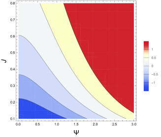
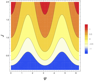
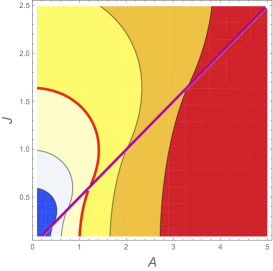
The half-plane (A,J>0)𝐴𝐽0(A,\,\,J>0) is divided by the curves F(J,A)=0𝐹𝐽𝐴0F(J,A)=0 and A=2J𝐴2𝐽A=2J into regions with different asymptotic behaviour of Z2(A,J)subscript𝑍2𝐴𝐽Z_{2}(A,J) at large N𝑁N, see Fig. 1.

Refer to caption

A        Refer to captionB

Refer to captionC        Refer to caption

Figure 1: Contour plots for the function F(A,J)𝐹𝐴𝐽F(A,J): A) for A/2J<1𝐴2𝐽1A/2J<1 and B) A/2J>1𝐴2𝐽1A/2J>1 as function of Ψ,JΨ𝐽\Psi,J and ψ,J𝜓𝐽\psi,J, respectively. C)The contour plot for F(A,J)𝐹𝐴𝐽F(A,J) as function of A𝐴A and J𝐽J. The magenta line shows the change of regimes and the red one shows the change of sign of F(A,J)𝐹𝐴𝐽F(A,J)

4 Quartic case

4.1 Partition function

Let us first consider the partition function for the quartic interaction

Z4(J)=N2π𝑑y𝑑xexp{N𝔖4},J>0,formulae-sequencesubscript𝑍4𝐽𝑁2𝜋differential-d𝑦differential-d𝑥𝑁subscript𝔖4𝐽0Z_{4}(J)=\frac{N}{2\pi}\int dy\int dx\,\exp\{N\mathfrak{S}_{4}\},\,\,\,\,\,J>0, (30)

where

𝔖4=J24x4+ixy+logy+logi.subscript𝔖4superscript𝐽24superscript𝑥4𝑖𝑥𝑦𝑦𝑖\mathfrak{S}_{4}=-\frac{J^{2}}{4}x^{4}+ixy+\log y+\log i. (31)

The stationary points are derived from equations

J2x3+iysuperscript𝐽2superscript𝑥3𝑖𝑦\displaystyle-J^{2}x^{3}+iy =\displaystyle= 0,0\displaystyle 0, (32)
1y+ix1𝑦𝑖𝑥\displaystyle\frac{1}{y}+ix =\displaystyle= 0.0\displaystyle 0. (33)

The solutions are

(𝔵0(1),𝔶0(1))subscriptsuperscript𝔵10subscriptsuperscript𝔶10\displaystyle(\mathfrak{x}^{(1)}_{0},\mathfrak{y}^{(1)}_{0}) =\displaystyle= (eiπ42J,2Jeiπ4),superscript𝑒𝑖𝜋42𝐽2𝐽superscript𝑒𝑖𝜋4\displaystyle\left(-\frac{e^{\frac{i\pi}{4}}}{\sqrt{2J}},-\sqrt{2J}e^{\frac{i\pi}{4}}\right), (34)
(𝔵0(2),𝔶0(2))subscriptsuperscript𝔵20subscriptsuperscript𝔶20\displaystyle(\mathfrak{x}^{(2)}_{0},\mathfrak{y}^{(2)}_{0}) =\displaystyle= (eiπ42J,2Jeiπ4),superscript𝑒𝑖𝜋42𝐽2𝐽superscript𝑒𝑖𝜋4\displaystyle\left(\frac{e^{\frac{i\pi}{4}}}{\sqrt{2J}},\sqrt{2J}e^{\frac{i\pi}{4}}\right), (35)
(𝔵0(3),𝔶0(3))subscriptsuperscript𝔵30subscriptsuperscript𝔶30\displaystyle(\mathfrak{x}^{(3)}_{0},\mathfrak{y}^{(3)}_{0}) =\displaystyle= (ei3π42J,2Jei3π4),superscript𝑒𝑖3𝜋42𝐽2𝐽superscript𝑒𝑖3𝜋4\displaystyle\left(-\frac{e^{\frac{i3\pi}{4}}}{\sqrt{2J}},\sqrt{2J}e^{\frac{i3\pi}{4}}\right), (36)
(𝔵0(4),𝔶0(4))subscriptsuperscript𝔵40subscriptsuperscript𝔶40\displaystyle(\mathfrak{x}^{(4)}_{0},\mathfrak{y}^{(4)}_{0}) =\displaystyle= (ei3π42J,2Jei3π4).superscript𝑒𝑖3𝜋42𝐽2𝐽superscript𝑒𝑖3𝜋4\displaystyle\left(\frac{e^{\frac{i3\pi}{4}}}{\sqrt{2J}},-\sqrt{2J}e^{\frac{i3\pi}{4}}\right). (37)

Expanding around the stationary points we get

𝔖4(1)=𝔖0132iJ(x+eiπ42J)2+i(y+2Jeiπ4)22J+i(x+eiπ42J)(y+2Jeiπ4),subscriptsuperscript𝔖14subscript𝔖0132𝑖𝐽superscript𝑥superscript𝑒𝑖𝜋42𝐽2𝑖superscript𝑦2𝐽superscript𝑒𝑖𝜋422𝐽𝑖𝑥superscript𝑒𝑖𝜋42𝐽𝑦2𝐽superscript𝑒𝑖𝜋4\displaystyle\mathfrak{S}^{(1)}_{4}=\mathfrak{S}_{01}-\frac{3}{2}iJ\left(x+\frac{e^{\frac{i\pi}{4}}}{\sqrt{2J}}\right)^{2}+\frac{i\left(y+\sqrt{2J}e^{\frac{i\pi}{4}}\right)^{2}}{2J}+i\left(x+\frac{e^{\frac{i\pi}{4}}}{\sqrt{2J}}\right)\left(y+\sqrt{2J}e^{\frac{i\pi}{4}}\right),
𝔖01=log(2Jeiπ4)34,subscript𝔖012𝐽superscript𝑒𝑖𝜋434\displaystyle\mathfrak{S}_{01}=\log\left(-\sqrt{2J}e^{\frac{i\pi}{4}}\right)-\frac{3}{4}, (38)
𝔖4(2)=𝔖0232iJ(xeiπ42J)2+i(y2Jeiπ4)22J+i(xeiπ42J)(y2Jeiπ4),subscriptsuperscript𝔖24subscript𝔖0232𝑖𝐽superscript𝑥superscript𝑒𝑖𝜋42𝐽2𝑖superscript𝑦2𝐽superscript𝑒𝑖𝜋422𝐽𝑖𝑥superscript𝑒𝑖𝜋42𝐽𝑦2𝐽superscript𝑒𝑖𝜋4\displaystyle\mathfrak{S}^{(2)}_{4}=\mathfrak{S}_{02}-\frac{3}{2}iJ\left(x-\frac{e^{\frac{i\pi}{4}}}{\sqrt{2J}}\right)^{2}+\frac{i\left(y-\sqrt{2J}e^{\frac{i\pi}{4}}\right)^{2}}{2J}+i\left(x-\frac{e^{\frac{i\pi}{4}}}{\sqrt{2J}}\right)\left(y-\sqrt{2J}e^{\frac{i\pi}{4}}\right),
𝔖02=log(2Jeiπ4)34,subscript𝔖022𝐽superscript𝑒𝑖𝜋434\displaystyle\mathfrak{S}_{02}=\log\left(\sqrt{2J}e^{\frac{i\pi}{4}}\right)-\frac{3}{4}, (39)
𝔖4(3)=𝔖02+32iJ(x+e3iπ42J)2i(y2Je3iπ4)22J+i(x+e3iπ42J)(y2Je3iπ4),subscriptsuperscript𝔖34subscript𝔖0232𝑖𝐽superscript𝑥superscript𝑒3𝑖𝜋42𝐽2𝑖superscript𝑦2𝐽superscript𝑒3𝑖𝜋422𝐽𝑖𝑥superscript𝑒3𝑖𝜋42𝐽𝑦2𝐽superscript𝑒3𝑖𝜋4\displaystyle\mathfrak{S}^{(3)}_{4}=\mathfrak{S}_{02}+\frac{3}{2}iJ\left(x+\frac{e^{\frac{3i\pi}{4}}}{\sqrt{2J}}\right)^{2}-\frac{i\left(y-\sqrt{2J}e^{\frac{3i\pi}{4}}\right)^{2}}{2J}+i\left(x+\frac{e^{\frac{3i\pi}{4}}}{\sqrt{2J}}\right)\left(y-\sqrt{2J}e^{\frac{3i\pi}{4}}\right),
𝔖03=log(2Jei3π4)34,subscript𝔖032𝐽superscript𝑒𝑖3𝜋434\displaystyle\mathfrak{S}_{03}=\log\left(\sqrt{2J}e^{\frac{i3\pi}{4}}\right)-\frac{3}{4}, (40)
𝔖4(4)=𝔖02+32iJ(xe3iπ42J)2i(y+2Je3iπ4)22J+i(xe3iπ42J)(y+2Je3iπ4),subscriptsuperscript𝔖44subscript𝔖0232𝑖𝐽superscript𝑥superscript𝑒3𝑖𝜋42𝐽2𝑖superscript𝑦2𝐽superscript𝑒3𝑖𝜋422𝐽𝑖𝑥superscript𝑒3𝑖𝜋42𝐽𝑦2𝐽superscript𝑒3𝑖𝜋4\displaystyle\mathfrak{S}^{(4)}_{4}=\mathfrak{S}_{02}+\frac{3}{2}iJ\left(x-\frac{e^{\frac{3i\pi}{4}}}{\sqrt{2J}}\right)^{2}-\frac{i\left(y+\sqrt{2J}e^{\frac{3i\pi}{4}}\right)^{2}}{2J}+i\left(x-\frac{e^{\frac{3i\pi}{4}}}{\sqrt{2J}}\right)\left(y+\sqrt{2J}e^{\frac{3i\pi}{4}}\right),
𝔖04=log(2Jei3π4)34.subscript𝔖042𝐽superscript𝑒𝑖3𝜋434\displaystyle\mathfrak{S}_{04}=\log\left(-\sqrt{2J}e^{\frac{i3\pi}{4}}\right)-\frac{3}{4}. (41)

We note that the real parts of 𝔖0i,i=1,2,3,4formulae-sequencesubscript𝔖0𝑖𝑖1234\mathfrak{S}_{0i},\,i=1,2,3,4 are equal and all four points contribute to the partition function. These contributions are the following. Integrating near the first, second, third and fourth points

Z4(i)(J)=N2π𝑑y𝑑xexp{N𝔖(i)},superscriptsubscript𝑍4𝑖𝐽𝑁2𝜋differential-d𝑦differential-d𝑥𝑁superscript𝔖𝑖Z_{4}^{(i)}(J)=\frac{N}{2\pi}\int dy\int dx\,\exp\{N\mathfrak{S}^{(i)}\}, (42)

we get

Z4(1)(J)superscriptsubscript𝑍41𝐽\displaystyle Z_{4}^{(1)}(J) =\displaystyle= πe3N/4((1i)J2)NN,𝜋superscript𝑒3𝑁4superscript1𝑖𝐽2𝑁𝑁\displaystyle\frac{\pi e^{-3N/4}\left((-1-i)\sqrt{\frac{J}{2}}\right)^{N}}{N}, (43)
Z4(2)(J)superscriptsubscript𝑍42𝐽\displaystyle Z_{4}^{(2)}(J) =\displaystyle= πe3N/4((1+i)J2)NN,𝜋superscript𝑒3𝑁4superscript1𝑖𝐽2𝑁𝑁\displaystyle\frac{\pi e^{-3N/4}\left((1+i)\sqrt{\frac{J}{2}}\right)^{N}}{N}, (44)
Z4(3)(J)superscriptsubscript𝑍43𝐽\displaystyle Z_{4}^{(3)}(J) =\displaystyle= πe3N/4((1+i)J2)NN,𝜋superscript𝑒3𝑁4superscript1𝑖𝐽2𝑁𝑁\displaystyle\frac{\pi e^{-3N/4}\left((-1+i)\sqrt{\frac{J}{2}}\right)^{N}}{N}, (45)
Z4(4)(J~)superscriptsubscript𝑍44~𝐽\displaystyle Z_{4}^{(4)}(\tilde{J}) =\displaystyle= πe3N/4((1i)J2)NN.𝜋superscript𝑒3𝑁4superscript1𝑖𝐽2𝑁𝑁\displaystyle\frac{\pi e^{-3N/4}\left((1-i)\sqrt{\frac{J}{2}}\right)^{N}}{N}. (46)

Summing up over all critical points we obtain

Z4(J~)=i=14Z4(i)(J~)subscript𝑍4~𝐽superscriptsubscript𝑖14superscriptsubscript𝑍4𝑖~𝐽\displaystyle Z_{4}(\tilde{J})=\sum_{i=1}^{4}Z_{4}^{(i)}(\tilde{J}) =\displaystyle= e3N/4(J2)N((1i)N+(1+i)N+(1+i)N+(1i)N)superscript𝑒3𝑁4superscript𝐽2𝑁superscript1𝑖𝑁superscript1𝑖𝑁superscript1𝑖𝑁superscript1𝑖𝑁\displaystyle e^{-3N/4}(\sqrt{\frac{J}{2}})^{N}((-1-i)^{N}+(1+i)^{N}+(-1+i)^{N}+(1-i)^{N}) (55)
=\displaystyle= e3N/4JN/2{4,N=8n0,N=8n+10,N=8n+20,N=8n+34,,N=8n+40,N=8n+50,N=8n+60,N=8n+7.superscript𝑒3𝑁4superscript𝐽𝑁2cases4missing-subexpression𝑁8𝑛0missing-subexpression𝑁8𝑛10missing-subexpression𝑁8𝑛20missing-subexpression𝑁8𝑛34absent𝑁8𝑛40missing-subexpression𝑁8𝑛50missing-subexpression𝑁8𝑛60missing-subexpression𝑁8𝑛7\displaystyle e^{-3N/4}J^{N/2}\left\{\begin{array}[]{ccc}4,&&N=8n\\ 0,&&N=8n+1\\ 0,&&N=8n+2\\ 0,&&N=8n+3\\ -4,&,&N=8n+4\\ 0,&&N=8n+5\\ 0,&&N=8n+6\\ 0,&&N=8n+7\\ \end{array}\right..

4.2 Generating function

The generating function depending on A𝐴A and J𝐽J is defined as

Z4(A,J)=N2π𝑑y𝑑xexp{NS4(A,J)},J>0formulae-sequencesubscript𝑍4𝐴𝐽𝑁2𝜋differential-d𝑦differential-d𝑥𝑁subscript𝑆4𝐴𝐽𝐽0Z_{4}(A,J)=\frac{N}{2\pi}\int dy\int dx\,\exp\{NS_{4}(A,J)\},\,\,\,\,\,J>0 (56)

where

S4(A,J)=J2x44+ixy+log(iy+A).subscript𝑆4𝐴𝐽superscript𝐽2superscript𝑥44𝑖𝑥𝑦𝑖𝑦𝐴S_{4}(A,J)=-J^{2}\frac{x^{4}}{4}+ixy+\log(iy+A). (57)

We can rewrite this expression as

Z4(A,J)=N2πJN/2𝑑y𝑑x(iy+AJ)Nexp{x44+ixy}subscript𝑍4𝐴𝐽𝑁2𝜋superscript𝐽𝑁2differential-d𝑦differential-d𝑥superscript𝑖𝑦𝐴𝐽𝑁superscript𝑥44𝑖𝑥𝑦Z_{4}(A,J)=\frac{N}{2\pi}J^{N/2}\int dy\int dx\,(iy+\frac{A}{\sqrt{J}})^{N}\exp\{-\frac{x^{4}}{4}+ixy\} (58)
=N2πJN/2dydxexp{NS4(A~),J>0,=\frac{N}{2\pi}J^{N/2}\int dy\int dx\,\exp\{NS_{4}(\tilde{A}),\,\,\,\,\,J>0,

where

S4(A~)=x44+ixy+log(iy+A~)subscript𝑆4~𝐴superscript𝑥44𝑖𝑥𝑦𝑖𝑦~𝐴S_{4}(\tilde{A})=-\frac{x^{4}}{4}+ixy+\log(iy+\tilde{A}) (59)

and A~=A/J.~𝐴𝐴𝐽\tilde{A}=A/\sqrt{J}.

The stationary points are derived from equations

x3+iysuperscript𝑥3𝑖𝑦\displaystyle-x^{3}+iy =\displaystyle= 00\displaystyle 0 (60)
iA~+iy+ix𝑖~𝐴𝑖𝑦𝑖𝑥\displaystyle\frac{i}{\tilde{A}+iy}+ix =\displaystyle= 0,0\displaystyle 0, (61)

that give

x0(1)subscriptsuperscript𝑥10\displaystyle x^{(1)}_{0} =\displaystyle= 12M12K1,x0(2)=12M+12K1,12𝑀12subscript𝐾1subscriptsuperscript𝑥2012𝑀12subscript𝐾1\displaystyle\frac{1}{2}M-\frac{1}{2}K_{1},\,\,\,\,\,x^{(2)}_{0}=\frac{1}{2}M+\frac{1}{2}K_{1},
x0(3)subscriptsuperscript𝑥30\displaystyle x^{(3)}_{0} =\displaystyle= 12M12K2,x0(4)=12M+12K2,12𝑀12subscript𝐾2subscriptsuperscript𝑥4012𝑀12subscript𝐾2\displaystyle-\frac{1}{2}M-\frac{1}{2}K_{2},\,\,\,\,\,\,x^{(4)}_{0}=-\frac{1}{2}M+\frac{1}{2}K_{2}, (62)
y0(1)subscriptsuperscript𝑦10\displaystyle y^{(1)}_{0} =\displaystyle= i(K234A~+18K13+943K1P18M3+943MP+18323K1P+18323MP),𝑖subscript𝐾234~𝐴18superscriptsubscript𝐾13394subscript𝐾1𝑃18superscript𝑀3394𝑀𝑃18332subscript𝐾1𝑃18332𝑀𝑃\displaystyle i\left(K_{2}\frac{3}{4}\tilde{A}+\frac{1}{8}K_{1}^{3}+\sqrt[3]{\frac{9}{4}}\frac{K_{1}}{P}-\frac{1}{8}M^{3}+\sqrt[3]{\frac{9}{4}}\frac{M}{P}+\frac{1}{8}\sqrt[3]{\frac{3}{2}}K_{1}P+\frac{1}{8}\sqrt[3]{\frac{3}{2}}MP\right),
y0(2)subscriptsuperscript𝑦20\displaystyle y^{(2)}_{0} =\displaystyle= i(34A~18K13943K1P18M3+943MP18323K1P+18323MP),𝑖34~𝐴18superscriptsubscript𝐾13394subscript𝐾1𝑃18superscript𝑀3394𝑀𝑃18332subscript𝐾1𝑃18332𝑀𝑃\displaystyle i\left(\frac{3}{4}\tilde{A}-\frac{1}{8}K_{1}^{3}-\sqrt[3]{\frac{9}{4}}\frac{K_{1}}{P}-\frac{1}{8}M^{3}+\sqrt[3]{\frac{9}{4}}\frac{M}{P}-\frac{1}{8}\sqrt[3]{\frac{3}{2}}K_{1}P+\frac{1}{8}\sqrt[3]{\frac{3}{2}}MP\right),
y0(3)subscriptsuperscript𝑦30\displaystyle y^{(3)}_{0} =\displaystyle= i(34A~+18K23+943K2P+18M3943MP+18323K2P18323MP),𝑖34~𝐴18superscriptsubscript𝐾23394subscript𝐾2𝑃18superscript𝑀3394𝑀𝑃18332subscript𝐾2𝑃18332𝑀𝑃\displaystyle i\left(\frac{3}{4}\tilde{A}+\frac{1}{8}K_{2}^{3}+\sqrt[3]{\frac{9}{4}}\frac{K_{2}}{P}+\frac{1}{8}M^{3}-\sqrt[3]{\frac{9}{4}}\frac{M}{P}+\frac{1}{8}\sqrt[3]{\frac{3}{2}}K_{2}P-\frac{1}{8}\sqrt[3]{\frac{3}{2}}MP\right),
y0(4)subscriptsuperscript𝑦40\displaystyle y^{(4)}_{0} =\displaystyle= i(34A~18K23943K2P+18M2943MP18323K2P18323MP),𝑖34~𝐴18superscriptsubscript𝐾23394subscript𝐾2𝑃18superscript𝑀2394𝑀𝑃18332subscript𝐾2𝑃18332𝑀𝑃\displaystyle i\left(\frac{3}{4}\tilde{A}-\frac{1}{8}K_{2}^{3}-\sqrt[3]{\frac{9}{4}}\frac{K_{2}}{P}+\frac{1}{8}M^{2}-\sqrt[3]{\frac{9}{4}}\frac{M}{P}-\frac{1}{8}\sqrt[3]{\frac{3}{2}}K_{2}P-\frac{1}{8}\sqrt[3]{\frac{3}{2}}MP\right), (63)

where

P𝑃\displaystyle P =\displaystyle= 327A~4256+9A~23,M=P183+2334P,3327superscript~𝐴42569superscript~𝐴2𝑀𝑃3183234𝑃\displaystyle\sqrt[3]{\sqrt{3}\sqrt{27\tilde{A}^{4}-256}+9\tilde{A}^{2}},\,\,\,\,M=\sqrt{\frac{P}{\sqrt[3]{18}}+\sqrt[3]{\frac{2}{3}}\frac{4}{P}},\,\,\,\,\, (64)
K1subscript𝐾1\displaystyle K_{1} =\displaystyle= 2A~MM2,K2=2A~MM2.2~𝐴𝑀superscript𝑀2subscript𝐾22~𝐴𝑀superscript𝑀2\displaystyle\sqrt{-\frac{2\tilde{A}}{M}-M^{2}},\,\,\,\,\,K_{2}=\sqrt{\frac{2\tilde{A}}{M}-M^{2}}. (65)

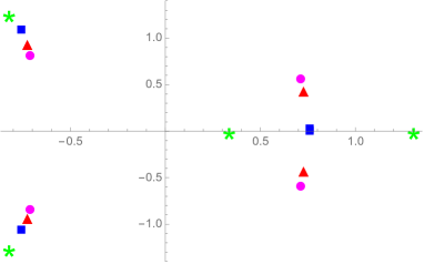
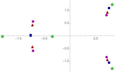
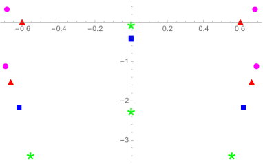
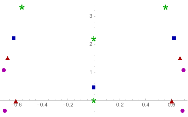
In Fig.2 we present the location of these roots.

  • We see that for |A~|<433/4~𝐴4superscript334|\tilde{A}|<\frac{4}{3^{3/4}} there are two pairs of complex conjugated x-roots: x0(2)=x¯0(1)subscriptsuperscript𝑥20subscriptsuperscript¯𝑥10x^{(2)}_{0}=\bar{x}^{(1)}_{0}, x0(4)=x¯0(3)subscriptsuperscript𝑥40subscriptsuperscript¯𝑥30x^{(4)}_{0}=\bar{x}^{(3)}_{0} and two pairs of y-roots related as: y0(2)=y¯0(1)subscriptsuperscript𝑦20subscriptsuperscript¯𝑦10y^{(2)}_{0}=-\bar{y}^{(1)}_{0}, y0(4)=y¯0(3)subscriptsuperscript𝑦40subscriptsuperscript¯𝑦30y^{(4)}_{0}=-\bar{y}^{(3)}_{0}. We call this domain the 𝔗𝔗\mathfrak{T} domain (the trigonometrical domain).

  • For A~=±433/4~𝐴plus-or-minus4superscript334\tilde{A}=\pm\frac{4}{3^{3/4}} we have for x-roots: one pair of complex conjugated values x0(1)=x¯0(2)subscriptsuperscript𝑥10subscriptsuperscript¯𝑥20x^{(1)}_{0}=\bar{x}^{(2)}_{0} and one pair of equal reals x0(3)=x0(4)subscriptsuperscript𝑥30subscriptsuperscript𝑥40x^{(3)}_{0}=x^{(4)}_{0}, and for y-roots: one pair of y-roots related as y0(2)=y¯0(1)subscriptsuperscript𝑦20subscriptsuperscript¯𝑦10y^{(2)}_{0}=-\bar{y}^{(1)}_{0} and one pair of equal pure imaginary y0(3)=y0(4)subscriptsuperscript𝑦30subscriptsuperscript𝑦40y^{(3)}_{0}=y^{(4)}_{0}. This is the critical domain \mathfrak{C}.

  • For A~>433/4~𝐴4superscript334\tilde{A}>\frac{4}{3^{3/4}} we have for x-roots: one pair of complex conjugated values x0(1)=x¯0(2)subscriptsuperscript𝑥10subscriptsuperscript¯𝑥20x^{(1)}_{0}=\bar{x}^{(2)}_{0} and one pair of non-equal reals x0(3)<x0(4)<0subscriptsuperscript𝑥30subscriptsuperscript𝑥400x^{(3)}_{0}<x^{(4)}_{0}<0, and for y-roots: one pair of y-roots related as : y0(2)=y¯0(1)subscriptsuperscript𝑦20subscriptsuperscript¯𝑦10y^{(2)}_{0}=-\bar{y}^{(1)}_{0} and one pair of non-equal pure imaginary 0<Imy0(4)<Imy0(3)0Imsubscriptsuperscript𝑦40Imsubscriptsuperscript𝑦300<\text{Im}\,y^{(4)}_{0}<\text{Im}\,y^{(3)}_{0}. This is the hyperbolic domain +subscript\mathfrak{H}_{+}.

    For A~<433/4~𝐴4superscript334\tilde{A}<-\frac{4}{3^{3/4}} we have for x-roots: one pair of complex conjugated values x0(3)=x¯0(4)subscriptsuperscript𝑥30subscriptsuperscript¯𝑥40x^{(3)}_{0}=\bar{x}^{(4)}_{0} and one pair of non-equal reals 0<x0(1)<x0(2)0subscriptsuperscript𝑥10subscriptsuperscript𝑥200<x^{(1)}_{0}<x^{(2)}_{0}, and for y-roots: one pair of y-roots related as y0(3)=y¯0(3)subscriptsuperscript𝑦30subscriptsuperscript¯𝑦30y^{(3)}_{0}=-\bar{y}^{(3)}_{0} and one pair of non-equal pure imaginary Imy0(2)<Imy0(1)<0Imsubscriptsuperscript𝑦20Imsubscriptsuperscript𝑦100\text{Im}\,y^{(2)}_{0}<\text{Im}\,y^{(1)}_{0}<0. This is the hyperbolic domain subscript\mathfrak{H}_{-}.

  • The boundaries of the ±subscriptplus-or-minus\mathfrak{H}_{\pm} and 𝔗±subscript𝔗plus-or-minus\mathfrak{T}_{\pm} come from solutions of the equation

    K2=02A~M3=0subscript𝐾202~𝐴superscript𝑀30K_{2}=0\Rightarrow 2\tilde{A}-M^{3}=0 (66)

    or explicitly

    144A~2(81A~4768+9A~2)=(23(81A~4768+9A~2)2/3+833)3.144superscript~𝐴281superscript~𝐴47689superscript~𝐴2superscript32superscript81superscript~𝐴47689superscript~𝐴2238333144\tilde{A}^{2}\left(\sqrt{81\tilde{A}^{4}-768}+9\tilde{A}^{2}\right)=\left(\sqrt[3]{2}\left(\sqrt{81\tilde{A}^{4}-768}+9\tilde{A}^{2}\right)^{2/3}+8\sqrt[3]{3}\right)^{3}. (67)

    The solutions of (67) are

    A~0=±433/4±1.755.subscript~𝐴0plus-or-minus4superscript334plus-or-minus1.755\tilde{A}_{0}=\pm\frac{4}{3^{3/4}}\approx\pm 1.755. (68)
Refer to caption

              Refer to caption
Refer to caption                           Refer to caption

Refer to caption

              Refer to caption
Refer to caption                           Refer to caption

Figure 2: Location of stationary points (x0(i)(A~),y0(i)(A~)),i=1,2,3,4formulae-sequencesubscriptsuperscript𝑥𝑖0~𝐴subscriptsuperscript𝑦𝑖0~𝐴𝑖1234(x^{(i)}_{0}(\tilde{A}),\,y^{(i)}_{0}(\tilde{A})),\,\,i=1,2,3,4, depending on A~~𝐴\tilde{A}.

Expanding the action (57) around these stationary points we get

S4(A,J)|xx0(i)S4(i)(A,J)evaluated-atsubscript𝑆4𝐴𝐽similar-to𝑥superscriptsubscript𝑥0𝑖subscriptsuperscript𝑆𝑖4𝐴𝐽\displaystyle S_{4}(A,J)\Big{|}_{x\sim x_{0}^{(i)}}\approx S^{(i)}_{4}(A,J) =\displaystyle= S0i(A,J)+Qαβ(i)(A~)X(i)αX(i)β,Xα=(X,Y),i=1,2,3,4formulae-sequencesubscript𝑆0𝑖𝐴𝐽subscriptsuperscript𝑄𝑖𝛼𝛽~𝐴superscript𝑋𝑖𝛼superscript𝑋𝑖𝛽superscript𝑋𝛼𝑋𝑌𝑖1234\displaystyle S_{0i}(A,J)+Q^{(i)}_{\alpha\beta}(\tilde{A})X^{(i)\alpha}X^{(i)\beta},\,\,\,X^{\alpha}=(X,Y),\,\,\,i=1,2,3,4
X𝑋\displaystyle X =\displaystyle= xx0(i),Y=yy0(i),𝑥superscriptsubscript𝑥0𝑖𝑌𝑦superscriptsubscript𝑦0𝑖\displaystyle x-x_{0}^{(i)},\,\,\,\,Y=y-y_{0}^{(i)}, (69)

where

S0i(A,J)subscript𝑆0𝑖𝐴𝐽\displaystyle S_{0i}(A,J) =\displaystyle= S0i(A~)+logJ,subscript𝑆0𝑖~𝐴𝐽\displaystyle S_{0i}(\tilde{A})+\log\sqrt{J}, (70)
S0i(A~)subscript𝑆0𝑖~𝐴\displaystyle S_{0i}(\tilde{A}) =\displaystyle= x0(i)42+ix0(i)y0(i)+log(iy0(i)+A~).\displaystyle-\frac{x^{(i)}_{0}\,{}^{4}}{2}+ix^{(i)}_{0}y^{(i)}_{0}+\log(iy^{(i)}_{0}+\tilde{A}). (71)

We have two types of solutions: trigonometric in the region 𝔗𝔗{\mathfrak{T}} and hyperbolic in the region {\mathfrak{H}} of the real line. In the region 𝔗𝔗{\mathfrak{T}} there are two pairs of complex conjugated roots and in the region {\mathfrak{H}} there is one pair of the complex conjugated and two reals roots of (60).

In the domain 𝔗𝔗{\mathfrak{T}} the real parts of S01(A~)subscript𝑆01~𝐴S_{01}(\tilde{A}) and S02(A~)subscript𝑆02~𝐴S_{02}(\tilde{A}), and the real parts of S03(A~)subscript𝑆03~𝐴S_{03}(\tilde{A}) and S04(A~)subscript𝑆04~𝐴S_{04}(\tilde{A}) coincide,

Re[S01(A~)]Redelimited-[]subscript𝑆01~𝐴\displaystyle\text{Re}[S_{01}(\tilde{A})] =\displaystyle= Re[S02(A~)],Redelimited-[]subscript𝑆02~𝐴\displaystyle\text{Re}[S_{02}(\tilde{A})], (72)
Re[S03(A~)]Redelimited-[]subscript𝑆03~𝐴\displaystyle\text{Re}[S_{03}(\tilde{A})] =\displaystyle= Re[S04(A~)].Redelimited-[]subscript𝑆04~𝐴\displaystyle\text{Re}[S_{04}(\tilde{A})]. (73)

It turns out that

Re[S01(A~)]Redelimited-[]subscript𝑆01~𝐴\displaystyle\text{Re}[S_{01}(\tilde{A})] >\displaystyle> Re[S03(A~)], forA~𝔗,Redelimited-[]subscript𝑆03~𝐴 for~𝐴subscript𝔗\displaystyle\text{Re}[S_{03}(\tilde{A})],\,\,\,{\mbox{ for}}\,\,\tilde{A}\in\mathfrak{T}_{-}, (74)
Re[S01(A~)]Redelimited-[]subscript𝑆01~𝐴\displaystyle\text{Re}[S_{01}(\tilde{A})] <\displaystyle< Re[S03(A~)], forA𝔗+,Redelimited-[]subscript𝑆03~𝐴 for𝐴subscript𝔗\displaystyle\text{Re}[S_{03}(\tilde{A})],\,\,\,{\mbox{ for}}\,\,A\in\mathfrak{T}_{+}, (75)

𝔗subscript𝔗minus-or-plus\mathfrak{T}_{\mp} are parts of 𝔗𝔗\mathfrak{T} where A~<0~𝐴0\tilde{A}<0 and A~>0~𝐴0\tilde{A}>0, respectively. In \mathfrak{H} we have

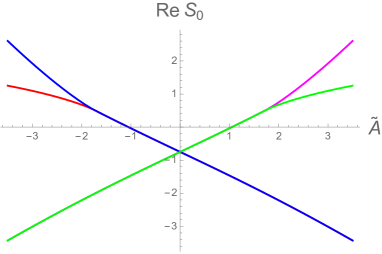
Re[S02(A~)]Redelimited-[]subscript𝑆02~𝐴\displaystyle\text{Re}[S_{02}(\tilde{A})] >\displaystyle> Re[S01(A~)]>Re[S03(A~)]=Re[S04(A~)], forA~,formulae-sequenceRedelimited-[]subscript𝑆01~𝐴Redelimited-[]subscript𝑆03~𝐴Redelimited-[]subscript𝑆04~𝐴 for~𝐴subscript\displaystyle\text{Re}[S_{01}(\tilde{A})]>\text{Re}[S_{03}(\tilde{A})]=\text{Re}[S_{04}(\tilde{A})],\,\,\,{\mbox{ for}}\,\,\tilde{A}\in\mathfrak{H}_{-}, (76)
Re[S03(A~)]Redelimited-[]subscript𝑆03~𝐴\displaystyle\text{Re}[S_{03}(\tilde{A})] >\displaystyle> Re[S04(A~)]>Re[S01(A~)]=Re[S02(A~)], forA~+,formulae-sequenceRedelimited-[]subscript𝑆04~𝐴Redelimited-[]subscript𝑆01~𝐴Redelimited-[]subscript𝑆02~𝐴 for~𝐴subscript\displaystyle\text{Re}[S_{04}(\tilde{A})]>\text{Re}[S_{01}(\tilde{A})]=\text{Re}[S_{02}(\tilde{A})],\,\,\,{\mbox{ for}}\,\,\tilde{A}\in\mathfrak{H}_{+},

subscriptminus-or-plus\mathfrak{H}_{\mp} are parts of \mathfrak{H} where A~<0~𝐴0\tilde{A}<0 and A~>0~𝐴0\tilde{A}>0, respectively, see Fig.3.

Refer to caption
Refer to caption
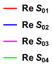
Figure 3: Values of Re[S0i(A~)],i=1,2,3,4formulae-sequenceRedelimited-[]subscript𝑆0𝑖~𝐴𝑖1234\text{Re}[S_{0i}(\tilde{A})],i=1,2,3,4 for arbitrary A~~𝐴\tilde{A}

In Fig.3 we present the dependence of the Re[S0i(A~)]Redelimited-[]subscript𝑆0𝑖~𝐴\text{Re}[S_{0i}(\tilde{A})], i=1,2,3,4𝑖1234i=1,2,3,4, on A~~𝐴\tilde{A}.

The quadratic forms have the following coefficients

Q11(i)=32x0(i),2Q12(i)=i,Q22(i)=12(A~+iy0(i))2\displaystyle Q^{(i)}_{11}=-\frac{3}{2}x^{(i)}_{0}\,{}^{2},\,\,\,\,Q^{(i)}_{12}=i,\,\,\,\,Q^{(i)}_{22}=\frac{1}{2\left(\tilde{A}+iy^{(i)}_{0}\right){}^{2}} (77)

and integrating over x𝑥x and y𝑦y we get the prefactor

Φ(k)=2πN13x0(k)2(A~+iy0(k))2,\Phi^{(k)}=\frac{2\pi}{N\sqrt{1-\frac{3x_{0}^{(k)}\,{}^{2}}{\left(\tilde{A}+iy_{0}^{(k)}\right){}^{2}}}}, (78)

that can be written in the form

Φ(k)=R(k)eiϕ(k),R(k)>0,   0ϕ(k)2π,formulae-sequencesuperscriptΦ𝑘superscript𝑅𝑘superscript𝑒𝑖superscriptitalic-ϕ𝑘formulae-sequencesuperscript𝑅𝑘0   0superscriptitalic-ϕ𝑘2𝜋\Phi^{(k)}=R^{(k)}e^{i\phi^{(k)}},\,\,\,\,\,R^{(k)}>0,\,\,\,0\leq\phi^{(k)}\leq 2\pi, (79)

k=1,2,3,4𝑘1234k=1,2,3,4.

We can approximate the integral by the contributions of these four points,

Z4(A,J)=i=14Φ(i)eNS0i(A,J),subscript𝑍4𝐴𝐽superscriptsubscript𝑖14superscriptΦ𝑖superscript𝑒𝑁subscript𝑆0𝑖𝐴𝐽\displaystyle Z_{4}(A,J)=\sum_{i=1}^{4}\,\Phi^{(i)}e^{NS_{0i}(A,J)}, (80)

but according to the inequalities (74) (see Fig.3) in the region subscript\mathfrak{H}_{-} the contribution from the second point (x0(2),y0(2))subscriptsuperscript𝑥20subscriptsuperscript𝑦20(x^{(2)}_{0},y^{(2)}_{0}) dominates, in the +subscript\mathfrak{H}_{+} the contribution from the third point (x0(3),y0(3))subscriptsuperscript𝑥30subscriptsuperscript𝑦30(x^{(3)}_{0},y^{(3)}_{0}) dominates. In 𝔗subscript𝔗\mathfrak{T}_{-} the contributions from the first and the second points, (x0(1),y0(1))subscriptsuperscript𝑥10subscriptsuperscript𝑦10(x^{(1)}_{0},y^{(1)}_{0}) and (x0(2),y0(2))subscriptsuperscript𝑥20subscriptsuperscript𝑦20(x^{(2)}_{0},y^{(2)}_{0}) dominate, and in 𝔗+subscript𝔗\mathfrak{T}_{+} the contributions from the third and the forth points, (x0(3),y0(3))subscriptsuperscript𝑥30subscriptsuperscript𝑦30(x^{(3)}_{0},y^{(3)}_{0}) and (x0(4),y0(4))subscriptsuperscript𝑥40subscriptsuperscript𝑦40(x^{(4)}_{0},y^{(4)}_{0}) dominate. The final result is

Z4(A,J)subscript𝑍4𝐴𝐽\displaystyle Z_{4}(A,J) \displaystyle\approx P(AJ)eNF(A,J),𝑃𝐴𝐽superscript𝑒𝑁𝐹𝐴𝐽\displaystyle P(\frac{A}{\sqrt{J}})\,e^{NF(A,J)}, (81)

where

F(A,J)𝐹𝐴𝐽\displaystyle F(A,J) \displaystyle\approx {ReS01(AJ)+12logJ,A~𝔗ReS03(AJ)+12logJ,A~𝔗+ReS01(AJ)+12logJ,A~ReS03(AJ)+12logJ,A~+,casesResubscript𝑆01𝐴𝐽12𝐽~𝐴subscript𝔗Resubscript𝑆03𝐴𝐽12𝐽~𝐴subscript𝔗Resubscript𝑆01𝐴𝐽12𝐽~𝐴subscriptResubscript𝑆03𝐴𝐽12𝐽~𝐴subscript\displaystyle\left\{\begin{array}[]{cc}\text{Re}S_{01}(\frac{A}{\sqrt{J}})+\frac{1}{2}\log J,&\,\tilde{A}\in\mathfrak{T}_{-}\\ \text{Re}S_{03}(\frac{A}{\sqrt{J}})+\frac{1}{2}\log J,&\,\tilde{A}\in\mathfrak{T}_{+}\\ \text{Re}S_{01}(\frac{A}{\sqrt{J}})+\frac{1}{2}\log J,&\tilde{A}\in\mathfrak{H}_{-}\\ \text{Re}S_{03}(\frac{A}{\sqrt{J}})+\frac{1}{2}\log J,&\tilde{A}\in\mathfrak{H}_{+}\end{array}\right., (86)

and

P(A~)={2R(1)(A~)cos(ϕ(1)(A~)+NImS01(A~)),A~𝔗2R(3)(A~)cos(ϕ(3)(A~)+NImS03(A~)),A~𝔗+2R(1)(A~),A~2R(3)(A~),A~+.𝑃~𝐴cases2superscript𝑅1~𝐴superscriptitalic-ϕ1~𝐴𝑁Imsubscript𝑆01~𝐴~𝐴subscript𝔗2superscript𝑅3~𝐴superscriptitalic-ϕ3~𝐴𝑁Imsubscript𝑆03~𝐴~𝐴subscript𝔗2superscript𝑅1~𝐴~𝐴subscript2superscript𝑅3~𝐴~𝐴subscript\displaystyle P(\tilde{A})=\left\{\begin{array}[]{cc}2R^{(1)}(\tilde{A})\cos(\phi^{(1)}(\tilde{A})+N\text{Im}S_{01}(\tilde{A})),&\,\tilde{A}\in\mathfrak{T}_{-}\\ 2R^{(3)}(\tilde{A})\cos(\phi^{(3)}(\tilde{A})+N\text{Im}S_{03}(\tilde{A})),&\,\tilde{A}\in\mathfrak{T}_{+}\\ 2R^{(1)}(\tilde{A}),&\tilde{A}\in\mathfrak{H}_{-}\\ 2R^{(3)}(\tilde{A}),&\tilde{A}\in\mathfrak{H}_{+}\end{array}\right.. (91)
Refer to caption

        Refer to caption

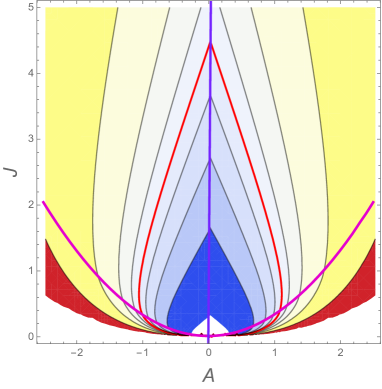
Figure 4: The equal level plot for free energy F(A,J)𝐹𝐴𝐽F(A,J) given by (86). The magenta line shows the phase transition line and the red one shows the change of sign of F(A,J)𝐹𝐴𝐽F(A,J)

In Fig.4 we plot the dependence of free energy F(A,J)𝐹𝐴𝐽F(A,J) on parameters A𝐴A and J𝐽J. We see that the half plane {(A,J):J>0}conditional-set𝐴𝐽𝐽0\{(A,J):\,J>0\} is divided into 8 regions by critical lines.

5 Conclusion

The formulation of the SYK model in real time is considered. The large N𝑁N asymptotic behavior of the generating functional Zq(A,J)subscript𝑍𝑞𝐴𝐽Z_{q}(A,J) in the zero dimensional SYK model with M=2𝑀2M=2 replicas has been studied and the phase transitions were investigated. There are 8 regions in the upper half plane {(A,J):J>0}conditional-set𝐴𝐽𝐽0\{(A,J):\,J>0\} with different behavior of the free energy F(A,J)𝐹𝐴𝐽F(A,J). For q=2𝑞2q=2 the critical curves are A2/J2=4,F(A,J)=0formulae-sequencesuperscript𝐴2superscript𝐽24𝐹𝐴𝐽0A^{2}/J^{2}=4,\,\,F(A,J)=0 and for q=4𝑞4q=4 the critical curves are A4/J2=44/33superscript𝐴4superscript𝐽2superscript44superscript33A^{4}/J^{2}=4^{4}/3^{3} as well as F(A,J)=0𝐹𝐴𝐽0F(A,J)=0 and A=0𝐴0A=0. For the arbitrary even q𝑞q the critical curve is given by the equation Aq/J2=qq/(q1)(q1)superscript𝐴𝑞superscript𝐽2superscript𝑞𝑞superscript𝑞1𝑞1A^{q}/J^{2}=q^{q}/(q-1)^{(q-1)}. It would be interesting to study the behavior in the model in this transition layer, i.e. an analogue of (29). The large N𝑁N behavior and phase transitions in the 0-dim SYK model in real time with arbitrary M>2𝑀2M>2 also deserves to study.

Acknowledgements

This work is supported by the Russian Science Foundation (project 14-50-00005, Steklov Mathematical Institute). We thank M. Khramtsov and M. Tikhanovskaya for useful discussions.

References

  • (1) S. Sachdev and J. Ye, ”Gapless spin fluid ground state in a random, quantum Heisenberg magnet,” Phys. Rev. Lett. 70 (1993) 3339, arXiv:cond-mat/9212030 [cond-mat].
  • (2) A. Kitaev, “A simple model of quantum holography,” KITP strings seminar and Entanglement 2015 program, (Feb. 12, April 7, and May 27, 2015) . http://online.kitp.ucsb.edu/online/entangled15/.
  • (3) S. Sachdev, “Bekenstein-Hawking Entropy and Strange Metals,” Phys. Rev. X 5, no. 4, 041025 (2015), [arXiv:1506.05111 [hep-th]].
  • (4) J. Polchinski and V. Rosenhaus, “The Spectrum in the Sachdev-Ye-Kitaev Model,” JHEP 1604, 001 (2016), [arXiv:1601.06768 [hep-th]].
  • (5) A. Jevicki, K. Suzuki and J. Yoon, “Bi-Local Holography in the SYK Model,” JHEP 1607, 007 (2016), [arXiv:1603.06246 [hep-th]].
  • (6) J. Maldacena and D. Stanford, “Remarks on the Sachdev-Ye-Kitaev model,” Phys. Rev. D 94, no. 10, 106002 (2016), [arXiv:1604.07818 [hep-th]].
  • (7) J. Maldacena, D. Stanford and Z. Yang, “Conformal symmetry and its breaking in two dimensional Nearly Anti-de-Sitter space,” PTEP 2016, no. 12, 12C104 (2016), [arXiv:1606.01857 [hep-th]].
  • (8) D. Bagrets, A. Altland and A. Kamenev, “Sachdev-Ye-Kitaev model as Liouville quantum mechanics,” Nucl. Phys. B 911, 191 (2016), [arXiv:1607.00694 [cond-mat.str-el]].
  • (9) K. Jensen, “Chaos in AdS2 Holography,” Phys. Rev. Lett.  117, no. 11, 111601 (2016), [arXiv:1605.06098 [hep-th]].
  • (10) J. Engelsoy, T. G. Mertens and H. Verlinde, “An investigation of AdS2 backreaction and holography,” JHEP 1607, 139 (2016), [arXiv:1606.03438 [hep-th]].
  • (11) J. S. Cotler et al., “Black Holes and Random Matrices,” JHEP 1705, 118 (2017), [arXiv:1611.04650 [hep-th]].
  • (12) D. J. Gross and V. Rosenhaus, “The Bulk Dual of SYK: Cubic Couplings,” JHEP 1705, 092 (2017), [arXiv:1702.08016 [hep-th]].
  • (13) D. J. Gross and V. Rosenhaus, “All point correlation functions in SYK,” JHEP 1712, 148 (2017), [arXiv:1710.08113 [hep-th]].
  • (14) A. Kitaev and S. J. Suh, “The soft mode in the Sachdev-Ye-Kitaev model and its gravity dual,” arXiv:1711.08467 [hep-th].
  • (15) V. S. Vladimirov, I. V. Volovich, ”Superanalysis. Differential calculus”, Theor. and Math. Phys., 59:1 (1984), 317-335; ”Superanalysis. II. Integral calculus”, Theor. and Math. Phys., 60:2 (1984), 743-765.
  • (16) Szego, G. Orthogonal Polynomials, 4th ed. Providence, RI: Amer. Math. Soc., 1975
  • (17) M. Wyman, ” The asymptotic behaviour of the Hermite polynomials”, Canad. J. Math., 15:332–349 (1963).
  • (18) D. Dominici, ”Asymptotic analysis of the Hermite polynomials from their differential - difference equation,” Journal of Difference Equations and Applications, 13, 1115-1128 (2007).