Optimization-based Motion Planning in Virtual Driving Scenarios with Application to Communicating Autonomous Vehicles

Abstract

The paper addresses the problem of providing suitable reference trajectories in motion planning problems for autonomous vehicles. Among the various approaches to compute a reference trajectory, our aim is to find those trajectories which optimize a given performance criterion, for instance fuel consumption, comfort, safety, time, and obey constraints, e.g. collision avoidance, safety regions, control bounds. This task can be approached by geometric shortest path problems or by optimal control problems, which need to be solved efficiently. To this end we use direct discretization schemes and model-predictive control in combination with sensitivity updates to predict optimal solutions in the presence of perturbations. Applications arising in autonomous driving are presented. In particular, a distributed control algorithm for traffic scenarios with several autonomous vehicles that use car-to-car communication is introduced.

1 Introduction

Virtual driving summarizes the ability to simulate vehicles in different driving scenarios on a computer. It is an important tool as it allows to analyze the dynamic behavior of a vehicle and the performance of driver assistance systems in parallel to the development process. The employment of virtual driving allows to reduce costs since simulations are less expensive and less time consuming than real test-drives. Moreover, virtual driving is particularly useful in scenarios that are potentially dangerous for human drivers such as collision avoidance scenarios or driving close to the physical limit. Moreover, the autonomous driving strategies can be developed and analyzed in virtual driving systems. However, virtual driving methods cannot fully replace physical testing since the virtual system is based on modeling assumptions that need to be verified in practice. Virtual driving simulators require models for the vehicle, the road, the environment (i.e. other cars, pedestrians, obstacles, …), components (i.e. sensors, cameras, …), and the driver (i.e. path planning, controller, driver assistance, …).

In this paper we focus on the driver, suitable path planning strategies, and control actions. Automatic path planning strategies are in the core of every virtual or real driving scenario for autonomous vehicles. Amongst the various approaches, e.g. sampling methods, shortest path problems and optimal control techniques, we focus on deterministic optimization-based methods such as geometric shortest paths, optimal control, and model-predictive control. While in virtual driving real-time capability is only of minor interest, in online computations it is the most important issue. In both cases robust methods are required that are capable of providing a suitable result reliably. A discussion of technical, legal, and social aspects of autonomous driving can be found in the recent book Maurer2015 .

This paper is organized as follows: Section 2 introduces working models for the vehicle, the road, obstacles, and the driver. In Section 3 approaches for optimization-based path planning are discussed. Amongst them we discuss geometric shortest path problems and optimal control approaches in more detail. Section 3.2 addresses collision detection methods. A model-predictive control scheme for communicating vehicles is suggested in Section 4. In Section 5 we discuss a feedback controller based on inverse kinematics for tracking a reference spline curve.

2 Modeling

Virtual driving requires a sufficiently realistic vehicle model, a model for its environment, and a driver model. Vehicle models exist in various levels of accuracy, ranging from simple point-mass models through single-track models to full car models. Which model to use depends on the effects that one likes to investigate. For handling purposes and online computations often a simple point-mass model or a single-track model with realistic tyre characteristics, compare Ger05a , are sufficiently accurate. For the investigation of dynamic load changes or vibrations a full car model in terms of a mechanical multi-body system is necessary, compare Ger03b ; Rill2011 for full car models and Burger2010 ; Burger2013 for applications with load excitations. Often, very detailed component models such as tyre models become necessary to investigate tyre-road contacts, compare Gallrein2007 ; Gallrein2014 .

Throughout the paper we use a simple kinematic car model, compare Rill2011 , since it is sufficient to introduce the basic ideas. The kinematic car model is valid for low lateral accelerations, low lateral tyre forces, and negligible side slip angles. It is not suitable for investigations close to the dynamic limit, though. The configuration of the car in a reference coordinate system is depicted in Figure 1. Herein, $\delta$ denotes the steering angle at the front wheels, $v$ the velocity of the car, $\psi$ the yaw angle, $\ell$ the distance from rear axle to front axle and $(x,y)$ the position of the midpoint of the rear axle.

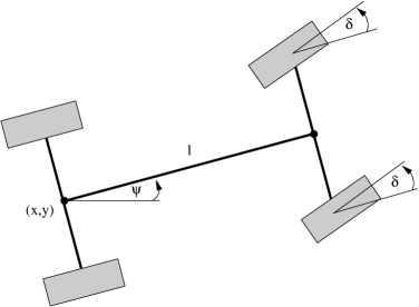
Figure 1: Configuration of the kinematic car model.

The equations of motion are derived as follows. The midpoint position and velocity of the rear axle of the car in the fixed reference system compute to

$$r_{R}=\left(\begin{array}[]{c}x\\ y\end{array}\right),\qquad v_{R}=\left(\begin{array}[]{c}x^{\prime}\\ y^{\prime}\end{array}\right).$$

The midpoint position and velocity of the front axle of the car in the fixed reference system compute to

$$r_{F} = \left(\begin{array}[]{c}x_{F}\\ y_{F}\end{array}\right)=r_{R}+S(\psi)\left(\begin{array}[]{c}\ell\\ 0\end{array}\right)=\left(\begin{array}[]{c}x+\ell\cos\psi\\ y+\ell\sin\psi\end{array}\right),$$

$$v_{F} = \left(\begin{array}[]{c}x_{F}^{\prime}\\ y_{F}^{\prime}\end{array}\right)=\left(\begin{array}[]{c}x^{\prime}-\ell\psi^{\prime}\sin\psi\\ y^{\prime}+\ell\psi^{\prime}\cos\psi\end{array}\right),$$

where

$$S(\psi)=\left(\begin{array}[]{cc}\cos\psi&-\sin\psi\\ \sin\psi&\cos\psi\end{array}\right)$$ (4)

is a rotation matrix that describes the rotation of the car’s fixed coordinate system against the inertial coordinate system.

Under the assumption that the lateral velocity components at rear axle and front axle vanish, we have that $r_{R}$, if transformed to the car’s reference system, only has a velocity component in the longitudinal direction of the car, i.e.

$$\left(\begin{array}[]{c}v\\ 0\end{array}\right)=S(\psi)^{\top}v_{R}\quad\Longleftrightarrow\quad v_{R}=S(\psi)\left(\begin{array}[]{c}v\\ 0\end{array}\right)=\left(\begin{array}[]{c}v\cos\psi\\ v\sin\psi\end{array}\right).$$

This leads to the differential equations for the position $(x,y)$ of the midpoint of the rear axle:

$$x^{\prime}(t)=v(t)\cos\psi(t),\qquad y^{\prime}(t)=v(t)\sin\psi(t).$$

Under the assumption that the lateral velocity component at the front axle vanishes, we have

$$0=e_{q}^{\top}v_{F,b},$$

where $e_{q}=(-\sin\delta,\cos\delta)^{\top}$ denotes the lateral direction of the front axle and

$$v_{F,b}:=S(\psi)^{\top}v_{F}=\left(\begin{array}[]{c}v\\ \ell\psi^{\prime}\end{array}\right)$$

denotes the representation of the velocity $v_{F}$ in the car’s body fixed reference system. The equation $0=e_{q}^{\top}v_{F,b}$ yields the differential equation

$$\psi^{\prime}(t)=\frac{v(t)}{\ell}\tan\delta(t)$$

for the yaw angle $\psi$. In summary, given the velocity $v(t)$ and the steering angle $\delta(t)$, the car’s motion is given by the following system of differential equations:

$$x^{\prime}(t) = v(t)\cos\psi(t),$$ (5)

$$y^{\prime}(t) = v(t)\sin\psi(t),$$ (6)

$$\psi^{\prime}(t) = \frac{v(t)}{\ell}\tan\delta(t).$$ (7)

The steering angle and the velocity are typically bounded by $|\delta|\leq\delta_{max}$ and by $0\leq v\leq v_{max}$ with given bounds $\delta_{max}$ and $v_{max}$, respectively. Moreover, one or more of the following modifications and restrictions can be used to yield a more realistic motion of the car:

• Instead of controlling the velocity directly one often controls the acceleration by adding the differential equation

  $$v^{\prime}(t)=a(t)$$ (8)

  with bounds for the control $a$, i.e. $a_{min}\leq a\leq a_{max}$.

• In order to model a certain delay in controlling the velocity $v$, one can consider the following differential equation for $v$:

  $$v^{\prime}(t)=\frac{v_{d}(t)-v(t)}{T}\qquad(T>0)$$ (9)

  Herein, $v_{d}(t)$ is the reference (=desired) velocity viewed as a control input and $v$ is the actual velocity. The constant $T$ allows to influence the response time, i.e. the delay of $v$.

• Instead of controlling the steering angle directly one often controls the steering angle velocity by adding the differential equation

  $$\delta^{\prime}(t)=w(t)$$ (10)

  with bounds for the control $w$, i.e. $|w|\leq w_{max}$.

The car model derived in this section only provides a simple model, which is, however, very useful for path planning tasks. More detailed models can be found in Rill2011 .

3 Trajectory Optimization and Path Planning

3.1 Geometric Path Planning by Shortest Paths

A first approach towards the automatic path planning is based on purely geometric considerations, whereas the detailed dynamics of the vehicle are not taken into account in its full complexity. In fact, a shortest path is sought that connects two given points in a configuration space, e.g. vehicle positions, while taking into account a fixed number of obstacles. The result is a sequence of configuration points that need to be tracked by the vehicle. This simple, but robust and effective planning strategy turns out to be useful in the presence of complicated path constraints or many fixed obstacles that need to be avoided. The resulting path may serve as a reference path for inverse dynamics, a feedback tracking controller, or as an initial guess for more sophisticated optimization approaches from optimal control.

In summary, the following steps need to be performed in order to compute a trajectory from an initial position to a terminal position, while taking obstacles into account:

• Solve a collision-free geometric shortest path problem using Dijkstra’s algorithm. The shortest path consists of a sequence of way-points leading from the initial position to the terminal position.

• Interpolate the way-points by a cubic spline function (use a thinning algorithm if necessary).

• Use inverse kinematics based on the car model or a feedback controller to track the spline function.

The above steps are discussed step by step.

In a first attempt we focus on the two dimensional $(x,y)$-plane as the configuration space, which is often sufficient for autonomous ground-based vehicles. Note that the subsequent techniques can be easily extended to higher dimensions, e.g. in the context of robotics or flight path optimization.

Consider a two dimensional configuration space

$$Q=\{(x,y)^{\top}\in{\mathbb{R}}^{2}\;|\;x_{min}\leq x\leq x_{max},y_{min}\leq y\leq y_{max}\}=[x_{min},x_{max}]\times[y_{min},y_{max}],$$

which corresponds to the feasible $(x,y)$-positions of the reference point on the vehicle. An equidistant discretization of the configuration space reads as

$$Q_{h}=\{(x_{i},y_{j})^{\top}\in{\mathbb{R}}^{2}\;|\;x_{i}=x_{min}+ih_{x},\;y_{j}=y_{min}+jh_{x},i=0,\ldots,N_{x},j=0,\ldots,N_{y}\}$$

with step-sizes $h_{x}=(x_{max}-x_{min})/N_{x}$ and $h_{y}=(y_{max}-y_{min})/N_{y}$ and given numbers $N_{x},N_{y}\in{\mathbb{N}}$. Every grid point $q\in Q_{h}$ corresponds to the position of the vehicle’s reference point.

The geometric motion of the vehicle can be modeled in a very simplified way by transitions from a given grid point to neighboring grid points (called feasible transitions), see Figure 2.

Figure 2: Configuration space $Q_{h}$ and feasible transitions from a given grid point.

To this end, the discrete configuration space $Q_{h}$ together with the feasible transitions, defined by the discrete control set $\mathcal{U}_{h}$, define a directed graph $G=(Q_{h},E_{h})$ with nodes $Q_{h}$ and edges $E_{h}\subset Q_{h}\times Q_{h}$ such that

$$(\bar{q},q)\in E_{h}\qquad\Longleftrightarrow\qquad|x-\bar{x}|\leq h_{x}\mbox{ and }|y-\bar{x}|\leq h_{y},$$

where $\bar{q}=(\bar{x},\bar{y})^{\top}\in Q_{h}$ and $q=(x,y)^{\top}\in Q_{h}$. Note that the set of edges can be further reduced if only some of the transitions between grid points are permitted.

To each edge $(\bar{q},q)\in E_{h}$ of the graph we may assign the cost $c(\bar{q},q)=\|q-\bar{q}\|_{2}$ assuming that the time to move from node $\bar{q}$ to node $q$ is proportional to its Euclidean distance. More general costs may be assigned as well as long as they are non-negative. In particular we have to deal with infeasible nodes owing to collisions with obstacles. In order to avoid collisions, infeasible nodes can be eliminated from the set $Q_{h}$ beforehand or an infinite cost $c(\bar{q},q)$ can be assigned whenever $\bar{q}$ or $q$ are infeasible nodes. Whether a collision occurs can be checked with the technique of Section 3.2.

Given the graph $G$ and the non-negative cost function $c:E_{h}\rightarrow{\mathbb{R}}$, the task is to find a shortest path in $G$ leading from an initial node $q_{0}\in Q_{h}$ to a terminal node $q_{T}\in Q_{h}$. This can be achieved by Dijkstra’s shortest path algorithm or versions of it, compare Pap98 ; Kor08 . The algorithm, which exploits the dynamic programming principle, has a complexity of $\mathcal{O}(n^{2})$, where $n$ denotes the number of nodes in $G$. An efficient implementation of Dijkstra’s algorithm uses a priority queue, see Cormen2009 .

After a shortest path has been found, it can be further tuned in a post-processing process. The post-processing includes an optional thinning of the path as described in Nachtigal2015 , a spline interpolation, and the application of inverse kinematics or a tracking controller to follow the spline with the actual car model. A tracking controller based on the car model in (5)-(7) is designed in Section 5.

Figure 3 shows the result of the geometric shortest path planning approach for a double lane change maneuver. The trajectory is typically not optimal in the sense of optimal control, but may be acceptable for practical purposes or it may serve as an initial guess for an optimal control problem.

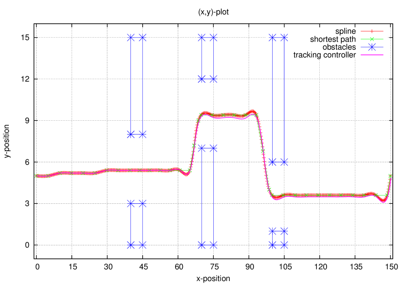
Figure 3: A car’s trajectory in the $(x,y)$-plane in the presence of obstacles starting at initial position $(0,5)$ and ending at position $(150,0)$: Shortest path, spline interpolation and tracked curve.

A more complicated track is depicted in Figure 4.

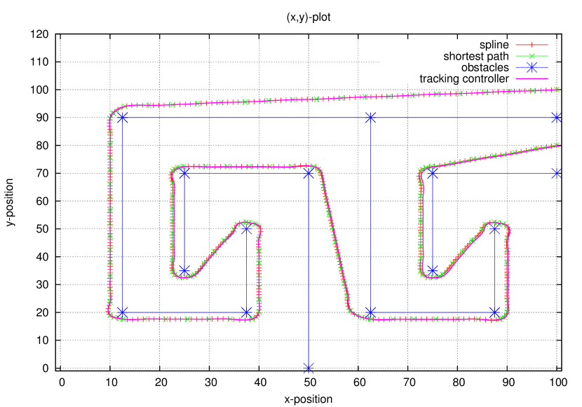
Figure 4: A car’s trajectory in the $(x,y)$-plane in the presence of obstacles starting at initial position $(100,100)$ and ending at position $(100,80)$: Shortest path, spline interpolation and tracked curve.

Although the geometric shortest path problem is robust and can handle fixed obstacles, moving obstacles (at the cost of an additional time state variable), and complicated obstacle geometries very well, it suffers from the disadvantage that, e.g. the steering angle $\delta$ cannot be constrained. For instance, the course in Figure 4 requires a maximum steering angle of 73 degrees, which is beyond the technical limit of a car. To avoid this remedy, it is possible to compute a cubic spline approximation in combination with inverse kinematics subject to constraints for the steering angle. Alternatively, one can modify the shortest path approach as follows: In the previous model, a purely geometric motion was considered that can be interpreted as controlling the motion in $x$- and $y$-direction independently from each other. This might be reasonable for omnidirectional robots, but it does not reflect the actual motion capabilities of a car with a steering device very well. To this end it is more realistic, although computationally more expensive, to work with a discretization of the dynamics (5)-(7) and the control set $\mathcal{U}:=[v_{min},v_{max}]\times[\delta_{min},\delta_{max}]$. This leads to a three dimensional configuration space $Q$ with points of type $q=(x,y,\psi)^{\top}$ subject to suitable bounds on the components. The discretized configuration space $Q_{h}$ is constructed as follows, where we use the explicit Euler method for simplicity: Let $\bar{q}=(\bar{x},\bar{y},\bar{\psi})^{\top}\in Q_{h}$ be arbitrary. Then $Q_{h}$ contains all the points $q=(x,y,\psi)^{\top}\in Q$ of type

$$q=\left(\begin{array}[]{c}x\\ y\\ \psi\end{array}\right)=\left(\begin{array}[]{c}\bar{x}+hv\cos\bar{\psi}\\ \bar{y}+hv\sin\bar{\psi}\\ \bar{\psi}+h\frac{v}{\ell}\tan\delta\end{array}\right)=:F(\bar{q},u)$$

with $u=(v,\delta)^{\top}\in\mathcal{U}_{h}$, where

$$\mathcal{U}_{h}:=\{(v_{i},\delta_{j})^{\top}\in{\mathbb{R}}^{2}\;|\;v_{i}=v_{min}+ih_{v},\;\delta_{j}=\delta_{min}+jh_{\delta},i=0,\ldots,N_{v},j=0,\ldots,N_{\delta}\}$$

is a discrete approximation to the set $\mathcal{U}$ with step-sizes $h_{v}=(v_{max}-v_{min})/N_{v}$ and $h_{\delta}=(\delta_{max}-\delta_{min})/N_{\delta}$.

Again, the discrete configuration space $Q_{h}$ together with the feasible transitions, defined by the discrete control set $\mathcal{U}_{h}$, define a directed graph $G=(Q_{h},E_{h})$ with nodes $Q_{h}$ and edges $E_{h}\subset Q_{h}\times Q_{h}$ such that

$$(\bar{q},q)\in E_{h}\qquad\Longleftrightarrow\qquad\exists u\in\mathcal{U}_{h}:q=F(\bar{q},u).$$

The graph is considerably larger than the previous one and the computational effort for solving the corresponding shortest path problem increases accordingly. Please note that time dependent obstacle motions can be incorporated at the dispense of an additional configuration variable which corresponds to the time. The shortest path approach essentially coincides with the dynamic programming approach, compare Bertsekas2012 .

3.2 Collision Detection

Collision detection is an important issue in robotics and autonomous systems and various approaches based on distance functions of convex bodies have been developed, see Gilbert1985 ; Johnson1985 ; Gilbert1988 . A smoothed distance measure was constructed in Escande2014 and can be used in gradient type optimization algorithms.

Often it is sufficient to approximate the vehicle with center $(x_{c},y_{c})$ and obstacles with centers $(x_{i},y_{i})$ by circles of radius $r$ and $r_{i}$, $i=1,\ldots,M$, respectively, and to impose state constraints of type

$$(x_{c}-x_{i})^{2}+(y_{c}-y_{i})^{2}\geq(r+r_{i})^{2},\qquad i=1,\ldots,M,$$

to prevent collisions. Herein, the center of the vehicle based on the configuration in Figure 1 is given by

$$r_{c}:=\left(\begin{array}[]{c}x_{c}\\ y_{c}\end{array}\right)=\left(\begin{array}[]{c}x\\ y\end{array}\right)+S(\psi)\left(\begin{array}[]{c}\ell/2\\ 0\end{array}\right).$$ (11)

Collision detection, taking the detailed shape of the vehicle and the obstacles into account, is much more involved, since it is not straightforward to compute the distance function for potentially non-convex bodies. We follow a technique in Landry2012 and assume that the shape of the vehicle of length $\ell$ and width $w$ in the two dimensional plane is given by a rectangle (w.r.t. to the vehicle’s coordinate system)

$$R=\{z\in{\mathbb{R}}^{2}\;|\;Az\leq b\},\qquad A=\left(\begin{array}[]{rr}1&0\\ -1&0\\ 0&1\\ 0&-1\end{array}\right),\ b=\left(\begin{array}[]{r}\ell/2\\ -\ell/2\\ w/2\\ -w/2\end{array}\right).$$

The rectangle moves along with the vehicle and its location at time $t$ is given by

$$R(t)=S(\psi(t))R+r_{c}(t)=\{z\in{\mathbb{R}}^{2}\;|\;AS(\psi(t))^{\top}z\leq b+AS(\psi(t))^{\top}r_{c}(t)\}$$

with $S$ from (4) and $r_{c}$ from (11). Let the $M$ obstacles at time $t$ be given by the union of convex polyhedra

$$Q_{i}(t):=\bigcup_{j=1}^{M_{i}}Q^{(i,j)}(t)\qquad\text{with}\qquad Q^{(i,j)}(t)=\{y\in{\mathbb{R}}^{2}\;|\;C^{(i,j)}(t)y\leq d^{(i,j)}(t)\},$$

where $M_{i}$ is the number of polyhedra in obstacle $Q_{i}$ and for $j=1,\ldots,M_{i}$, the matrix $C^{(i,j)}(t)\in{\mathbb{R}}^{q_{i,j}\times 2}$ and the vector $d^{(i,j)}(t)\in{\mathbb{R}}^{q_{i,j}}$ define the convex parts of the i-th obstacle at time $t$. Herein, $q_{i,j}$ is the number of facets in $Q^{(i,j)}$.

The vehicle and the obstacles do not collide at time $t$ if and only if

$$R(t)\cap Q^{(i,j)}(t)\,=\,\emptyset\qquad\forall j=1,\ldots,M_{i},i=1,\ldots,M.$$

This is equivalent to the infeasibility of the linear system

$$\left(\begin{array}[]{c}A(t)\\ C^{(i,j)}(t)\end{array}\right)\,z\,\leq\,\left(\begin{array}[]{c}b(t)\\ d^{(i,j)}(t)\end{array}\right),\quad\forall j=1,\ldots,M_{i},i=1,\ldots,M,$$ (12)

where $A(t):=AS(\psi(t))^{\top}$ and $b(t):=b+AS(\psi(t))^{\top}r_{c}(t)$. According to the Lemma of Gale the system (12) has no solution at time $t$ if and only if there exist vectors $w^{(i,j)}(t)\in{\mathbb{R}}^{4+q_{i,j}}$ such that

$$w^{(i,j)}(t)\,\geq\,0,\quad\left(\begin{array}[]{c}A(t)\\ C^{(i,j)}(t)\end{array}\right)^{\top}w^{(i,j)}(t)\,=\,0\quad\text{and}\quad\left(\begin{array}[]{c}b(t)\\ d^{(i,j)}(t)\end{array}\right)^{\top}w^{(i,j)}(t)<0.$$

Note that a scaled vector $\lambda w^{(i,j)}(t)$ with $\lambda>0$ satisfies the conditions as well, if $w^{(i,j)}(t)$ does so. Hence, we may bound the length of the components by one and impose the additional constraint $w^{(i,j)}(t)\leq e$, where $e=(1,\ldots,1)^{\top}$ denotes the vector of all ones of appropriate dimension.

This condition can be checked by solving the following linear program for all $j=1,\ldots,M_{i}$, $i=1,\ldots,M$, and all $t$:

Minimize

$$\left(\begin{array}[]{c}b(t)\\ d^{(i,j)}(t)\end{array}\right)^{\top}w^{(i,j)}(t)$$

subject to the constraints

$$0\,\leq\,w^{(i,j)}(t)\,\leq\,e,\qquad\left(\begin{array}[]{c}A(t)\\ C^{(i,j)}(t)\end{array}\right)^{\top}w^{(i,j)}(t)\,=\,0.$$

Note that the feasible sets of the linear programs are non-empty and compact and thus an optimal solution exists.

A collision does not occur, if the value function

$$\zeta^{(i,j)}(t):=\min\left\{\left(\begin{array}[]{c}b(t)^{\top}\\ d^{(i,j)}(t)\end{array}\right)^{\top}w\;\Bigg{|}\;0\,\leq w\,\leq\,e,\;\left(\begin{array}[]{c}A(t)\\ C^{(i,j)}(t)\end{array}\right)^{\top}w=0\right\}$$

is negative for all combinations $(i,j)$ and all $t$. Hence, collisions are avoided by imposing the non-linear and non-differentiable constraint

$$\sup_{t\in[0,t_{f}],(i,j)}\zeta^{(i,j)}(t)\leq-\varepsilon$$

for some $\varepsilon>0$ sufficiently small. Note that $\zeta^{(i,j)}$ implicitly depends on the vehicle’s state $(x,y,\psi)$.

As an alternative to the above linear programming approach, the Gilbert-Johnson-Keehrti algorithm from Gilbert1988 is frequently used in computer graphics and robotics for real-time collision detection. It uses Minkowski sums and convex hulls to compute the signed distance function between two polyhedral objects.

3.3 Optimal Drivers by Optimal Control

A virtual “optimal” driver can be modeled by means of a suitable optimal control problem, which fits into the following general class of parametric optimal control problems OCP($p$):

Minimize

$$\varphi(z(t_{f}),t_{f},p)+\int_{t_{0}}^{t_{f}}f_{0}(z(t),u(t),p)dt$$ (13)

subject to the constraints

$$z^{\prime}(t) =f(z(t),u(t),p) \mbox{a.e. in }[t_{0},t_{f}],$$ (14)

$$g(t,z(t),p) \leq 0 \mbox{in }[t_{0},t_{f}],$$ (15)

$$\psi(z(t_{0}),z(t_{f}),p) =0,$$ (16)

$$u(t) \in\mathcal{U} \mbox{a.e. in }[t_{0},t_{f}].$$ (17)

Herein, the objective function (13) typically consists of a linear combination of final time, steering effort and fuel consumption. The car model defines the differential equation in (14) for the state $z$ and control $u$, while road boundaries and stationary or moving obstacles lead to state constraints of type (15). Initial and terminal states of the vehicle at initial time $t_{0}$ and terminal time $t_{f}$ are limited by the constraint in (16). Finally, the control vector $u$ is restricted to the control set $\mathcal{U}$ in (17). The problem formulation may depend on a parameter vector $p$ that can be used to model perturbations or uncertainties, which enter the optimal control problem as parameters.

Given a nominal parameter $p^{*}$, various approaches exist to solve OCP($p^{*}$) numerically. The indirect solution approach exploits first order necessary optimality conditions, see Iof79 . The function space approach applies optimization procedures, i.e. gradient type methods in the function space setting of OCP($p^{*}$), compare Pol73 . For highly nonlinear problems with complicated state and control constraints, direct discretization methods, see Boc84 ; Bet01 ; Gerdts2012 , are often preferred owing to their flexibility and robustness. In the following example, we use an optimal control problem to model a parking maneuver of a car and solve the optimal control problem by the direct shooting method OCPID-DAE1, see OCPIDDAE1 .

Example 1 (Parking maneuver)

The task is to park a car in a parking space next to the car on the road. The car’s dynamics are given by (5)-(7), (8) and (10) with $\ell=2.7$ and width $b=1.8$. The state vector is given by $z=(x,y,\psi,v,\delta)^{\top}$ and the control vector by $u=(w,a)^{\top}$.

The steering angle velocity $w$ and the acceleration $a$ are restricted by the control constraints

$$w(t)\in[-0.5,0.5],\qquad a(t)\in[-0.5,0.5].$$ (18)

The steering angle $\delta$ is bounded by the state constraints

$$-\frac{\pi}{6}\leq\delta(t)\leq\frac{\pi}{6}.$$ (19)

The initial state of the car is given by

$$x(0)=2.5,\quad y(0)=1.5,\quad\psi(0)=v(0)=\delta(0)=0$$ (20)

and the terminal state by

$$x(t_{f})=-1.25,\quad y(t_{f})=-1.5,\quad\psi(t_{f})=v(t_{f})=\delta(t_{f})=0.$$ (21)

Moreover, the parking lot, which is located to the right of the car, is defined by the state constraints

$$y_{r}(t)\geq\eta(x_{r}(t))\quad\mbox{and}\quad y_{f}(t)\geq\eta(x_{f}(t)),$$ (22)

where

$$\left(\begin{array}[]{c}x_{r}(t)\\ y_{r}(t)\end{array}\right)=\left(\begin{array}[]{c}x(t)\\ y(t)\end{array}\right)+S(\psi(t))\left(\begin{array}[]{c}0\\ b/2\end{array}\right)\mbox{ and }\left(\begin{array}[]{c}x_{f}(t)\\ y_{f}(t)\end{array}\right)=\left(\begin{array}[]{c}x(t)\\ y(t)\end{array}\right)+S(\psi(t))\left(\begin{array}[]{c}\ell\\ b/2\end{array}\right)$$

denote the positions of the right front and right rear wheel centers, respectively, $S$ is the rotation matrix in (4) and $\eta$ is the piecewise defined and continuously differentiable function

$$\eta(x):=\left\{\begin{array}[]{ll}0,&\mbox{if }|x|\geq 2.5,\\ -3,&\mbox{if }|x|\leq 2.4,\\ -900(|x|-2.5)^{2}-6000(|x|-2.5)^{3},&\mbox{if }2.4<|x|<2.5.\end{array}\right.$$

Summarizing, the optimal control problem aims at minimizing a linear combination of final time and steering effort, that is

$$t_{f}+\int_{0}^{t_{f}}w(t)^{2}dt,$$

subject to the constraints (5)-(7), (8), (10), (18)-(22).

Figures 5-6 show the result of the direct shooting method OCPID-DAE1, see OCPIDDAE1 , with $N=101$ grid points and final time $t_{f}\approx 15.355$. Please note the 3 phases of the parking maneuver in Figure 5.

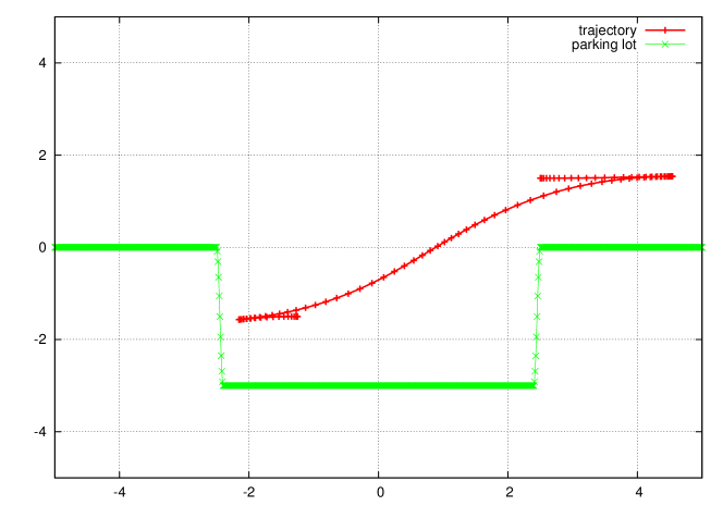
Figure 5: Trajectory $(x,y)$ for optimal parking maneuver.

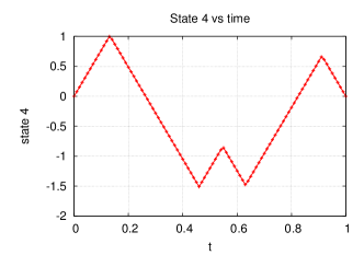
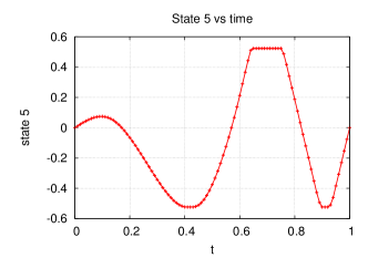
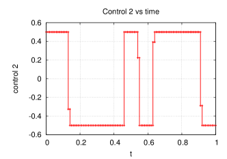
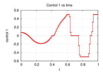
Figure 6: Velocity $v$ (state, top left), steering angle $\delta$ (state, top right), acceleration $a$ (control, bottom left), and steering angle velocity $w$ (control, bottom right) for optimal parking maneuver.

Figure 7 illustrates the motion of the car with some snapshots.

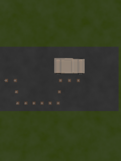
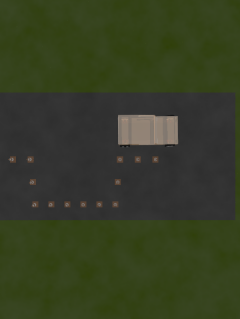
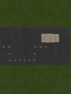
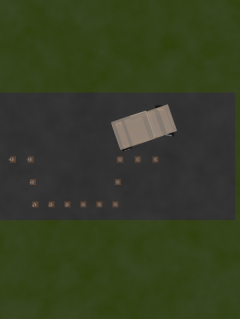
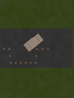
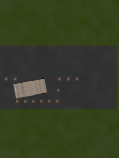
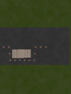
Figure 7: Snapshots of the car’s parking maneuver.

Example 1 illustrated how optimal control can be used to simulate a driver in an automatic parking maneuver. Now we like to investigate the influence of parameters. A parametric sensitivity analysis as in Mau01 for the nominal optimal control problem OCP($p^{*}$) with some nominal parameter $p^{*}$ allows to approximate the optimal solution $(z(p),u(p))$ of the perturbed problem OCP($p$) with $p$ close to $p^{*}$ locally by a first order Taylor approximation

$$z(p)\approx z(p^{*})+\frac{\partial z}{\partial p}(p^{*})(p-p^{*}),\quad u(p)\approx u(p^{*})+\frac{\partial u}{\partial p}(p^{*})(p-p^{*}).$$ (23)

This approximation holds for $p$ sufficiently close to $p^{*}$ under suitable assumptions on the nominal solution, i.e. first-order necessary conditions, strict complementarity, second-order sufficient conditions and linear independence constraint qualification have to hold. A similar approximation holds for discretized optimal control problems, compare Bue01a . These update formulas can be applied in real-time to update a nominal solution in the presence of perturbations in $p^{*}$. This idea can be exploited in multistep model-predictive control schemes as well, compare Palma2015 .

In the following example, we demonstrate the parametric sensitivity analysis for a collision avoidance maneuver.

Example 2 (Collision avoidance maneuver)

The task is to avoid a collision with a fixed obstacle that is blocking the right half of a straight road. The width of the road is $8$ meters and we aim to find the minimal distance $d$ such that an avoidance maneuver is possible with moderate steering effort. We introduce two perturbation parameters $p_{1}$ and $p_{2}$ with nominal values $p_{1}^{*}=p_{2}^{*}=0$ into the problem formulation. The first parameter $p_{1}$ models perturbations in the initial yaw angle. The second parameter $p_{2}$ models perturbations in the motion of the obstacle and allows the obstacle to move with a given velocity $v_{obs}=100$ [km/h] into a given direction with angle $\psi_{obs}=170$ [^∘].

The car’s dynamics are given by (5)-(7), (8) and (10) with $\ell=2.7$ and width $b=2$. The steering angle velocity $w$ and the acceleration $a$ are restricted by the control constraints

$$w(t)\in[-0.5,0.5],\qquad a(t)\in[-10.0,0.5].$$ (24)

The steering angle $\delta$ is bounded by the state constraints

$$-\frac{\pi}{6}\leq\delta(t)\leq\frac{\pi}{6}.$$ (25)

The initial state of the car is given by

$$x(0)=0,\quad y(0)=1.75,\quad\psi(0)=p_{1},\quad\delta(0)=0,\quad v(0)=27.78,$$ (26)

where $p_{1}$ is a perturbation parameter with nominal value $p_{1}^{*}=0$. The terminal state is given by

$$x(t_{f})=x_{obs}(t_{f})+3,\quad\psi(t_{f})=\delta(t_{f})=0$$ (27)

with

$$x_{obs}(t)=d+tp_{2}v_{obs}\cos\psi_{obs},\qquad y_{obs}(t)=3.5+tp_{2}v_{obs}\sin\psi_{obs}$$

and perturbation parameter $p_{2}$ with nominal value $p_{2}^{*}=0$. Note that the obstacle is not moving for the nominal parameter $p_{2}^{*}=0$.

Moreover, the obstacle is defined by the state constraints

$$s(x(t),x_{obs}(t),y_{obs}(t))+\frac{b}{2}\leq y(t)\leq 8-\frac{b}{2},$$ (28)

where $s$ is the piecewise defined and continuously differentiable function

$$s(x,d,h):=\left\{\begin{array}[]{ll}0,&\mbox{if }x<d,\\ 4h(x-d)^{3},&\mbox{if }d\leq x<d+0.5,\\ 4h(x-(d+1))^{3}+h,&\mbox{if }d+0.5\leq x<d+1,\\ h,&\mbox{if }x\geq d+1.\end{array}\right.$$

Summarizing, the optimal control problem aims at minimizing a linear combination of initial distance to the obstacle $d$ and steering effort, that is

$$d+18\int_{0}^{t_{f}}w(t)^{2}dt,$$

subject to the constraints (5)-(7), (8), (10), (24)-(28).

Figure 8 shows the output of the direct shooting method OCPID-DAE1, see OCPIDDAE1 , with $N=51$ grid points for the nominal optimal control problem with parameters $p_{1}^{*}=p_{2}^{*}=0$. The final time is $t_{f}\approx 1.00541$, the optimal distance to the obstacle amounts to $d\approx 19.62075$ and the acceleration is active at the lower bound with $a(t)=-10$ for all $t\in[0,t_{f}]$.

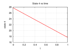
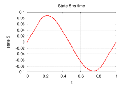
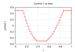
Figure 8: Trajectory $(x,y)$ (state, top), velocity $v$ (state, bottom left), steering angle $\delta$ (state, bottom middle) and steering angle velocity $w$ (control, bottom right) for optimal avoidance maneuver.

Figure 9 shows the sensitivities $\partial w/\partial p_{1}$ and $\partial w/\partial p_{2}$ of the nominal steering angle velocity $w(t)$ with respect to the parameters $p_{1}$ and $p_{2}$ for $t\in[0,t_{f}]$ .

Figure 9: Sensitivities of the steering angle velocity w.r.t. to $p_{1}$ (perturbation in initial yaw angle) and $p_{2}$ (perturbation of obstacle).

The sensitivities of the nominal final time $t_{f}$ with respect to $p_{1}$ and $p_{2}$ compute to

$$\frac{\partial t_{f}}{\partial p_{1}}\approx-1.66018,\qquad\frac{\partial t_{f}}{\partial p_{2}}\approx 0.50118.$$

The sensitivities of the nominal distance $d$ with respect to $p_{1}$ and $p_{2}$ compute to

$$\frac{\partial d}{\partial p_{1}}\approx-28.95949,\qquad\frac{\partial d}{\partial p_{2}}\approx 35.66225.$$

The sensitivities allow to predict the optimal solution under (small) perturbations using the Taylor approximation in (23). Figures 10-11 show the results of such a prediction for perturbations in the range of $p_{1}\in[-0.1,0.1]$ and $p_{2}\in[-0.1,0.1]$.

Figure 10: Perturbed trajectories (top), steering angle (bottom, left) and steering angle velocity (bottom, right) with sensitivity updates for perturbations $p_{1}\in[-0.1,0.1]$. Please note that not all perturbations are feasible.

Figure 11: Perturbed trajectories (top), steering angle (bottom, left) and steering angle velocity (bottom, right) with sensitivity updates for perturbations $p_{2}\in[-0.1,0.1]$. Please note that not all perturbations are feasible.

Naturally, these examples can only provide a small idea of how optimal control techniques can be used to control vehicles and many extensions and applications to more complicated scenarios exist. The problem of controlling an autonomous vehicle by means of optimal control in real-time was addressed in Schmidt2014b . Optimization based obstacle avoidance techniques can be found in Schmidt2014a ; Schmidt2014c .

A different approach that exploits ideas from reachability analysis was used in WooEsf:2012:IFA_4040 to design a controller for a scale car that drives autonomously on a given track. Reachable sets turn out to be a powerful tool to detect and avoid collisions and to investigate the influence on perturbations on the future dynamic behavior. A comprehensive overview can be found in Kurzhanski2014 . Althoff2010a uses reachability analysis with zonotopes and linearized dynamics for collision detection. Reachable set approximations through zonotopes have been obtained in Althoff2011f . Verification approaches for collision avoidance systems using reachable sets are investigated in Nielsson2014 ; Xausa2015 .

Virtual drives with gear shifts leading to mixed-integer optimal control problems have been considered in Ger05a ; Ger06b ; Kirches2010 .

4 Distributed Hierarchical Model-Predictive Control for Communicating Vehicles

While the trajectory generation for a single vehicle was in the focus of Section 3, we are now discussing control strategies for several autonomous vehicles that interact with each other. To this end we assume that we have $N\in{\mathbb{N}}$ vehicles that can communicate through suitable communication channels and exchange information on positions, velocities, and predicted future behavior. The aim is to efficiently control the vehicles in a self-organized and autonomous way without prescribing a route. We suggest to use a distributed model-predictive control (MPC) strategy and couple it with a priority list or hierarchy, compare Kianfar2012 ; Pannek2013 ; Gross2014 ; Findeisen2014 . The priority list will rank the vehicles in an adaptive way depending on the current driving situation and give highly ranked vehicles priority while driving. Vehicles with low priority have to obey the motion of vehicles with higher priority.

Model-predictive control is a well established feedback control paradigm, compare Gru11 for a detailed exposition and discussion of stability and robustness properties. The working principle of model predictive control is based on a repeated solution of (discretized) optimal control problems on a moving time horizon, see Figure 12. The model-predictive control scheme was used in Ger09 to simulate the drive on long tracks, see the picture on the right in Figure 12 for an example.

Figure 12: Model-predictive control scheme: Repeated optimization on a prediction horizon of length $T$ and control acting on a control interval of length $\tau$ (left). Application to a test-drive (right): Local solutions of the MPC scheme, compare Ger09 .

The MPC algorithm depends on a local time horizon of length $T>0$, sampling times $t_{i}$, $i\in{\mathbb{N}}_{0}$, and a shifting parameter $\tau>0$. On each local time horizon $[t_{i},t_{i}+T]$ an optimal control problem has to be solved for a given initial state, which may result from a measurement and represents the current state of the vehicle. Then the computed optimal control is implemented on the interval $[t_{i},t_{i}+\tau]$ and the state is measured again at the sampling time $t_{i+1}=t_{i}+\tau$. After that, the process is repeated on the shifted time interval $[t_{i+1},t_{i+1}+T]$. This control paradigm provides a feedback control, since it reacts on the actual state at the sampling times $t_{i}$, $i\in{\mathbb{N}}_{0}$. Moreover, the control paradigm is very flexible since control and state constraints and individual objectives can be considered in the local optimal control problems, compare Section 3.3.

The basic model-predictive control scheme has to be enhanced towards distributed vehicle systems. Herein, the computations take place on the individual vehicles and the relevant information is exchanged. In addition, a priority list has to be included.

4.1 Priority List

The priority list consists of a set of predefined rules to rank the vehicles. Vehicles with a lower priority have to take into account in their motion planning algorithm the motion of the vehicles with higher priority, while vehicles with the same priority can move independently, see Pannek2013 .

To simplify the computations we assume that each vehicle only considers its neighboring vehicles as potential obstacles in the state constraints, i.e. vehicles which are inside a certain communication radius or distance. Vehicles outside this neighborhood are ignored in the optimization process. For each of the $N\in{\mathbb{N}}$ vehicles we introduce the set

$$I_{NH}(i):=\left\{j\in\left\{1,\ldots,N\right\}\setminus\left\{i\right\}\mid j\text{ is a neighbor of }i\right\},$$

which contains the indexes of the neighbors of the $i$-th vehicle.

In order to avoid a conflict between vehicles, which could lead to a collision, we introduce a set of rules which assigns a distinct hierarchy level to each vehicle, i.e. every vehicle inside the $i$-th vehicle’s neighborhood has either a higher or lower hierarchy level than the $i$-th vehicle. The vehicle with the lower hierarchy level has to consider the safety boundary of the vehicles with a higher hierarchy level in terms of state constraints, while a vehicle with a higher priority is allowed to ignore the safety boundaries of neighboring vehicles with a lower priority. The set

$$I_{PR}(i):=\left\{j\in I_{NH}(i)\mid j\text{ has a higher priority than }i\right\}$$

contains all indexes of the neighboring vehicles of the $i$-th vehicle, which have a higher hierarchy level than the $i$-th vehicle. If a vehicle has the highest possible priority this set is empty, if it has the lowest hierarchy level it contains all neighboring vehicles. This approach is also able to handle vehicles, which are not part of the communication network, e.g. an ambulance or non autonomous vehicles, by giving those vehicles the highest priority. The rules may also have a certain priority, e.g. traffic rules may have a higher priority than mathematically motivated rules.

By this approach the computational effort is being reduced, because vehicles with no neighbors or vehicles with the highest hierarchy level are allowed to ignore other vehicles and are able to drive in an optimal way with fewer state constraints. It also reduces the potential for conflicts between vehicles, because of the distinct hierarchy. Depending on the scenario, the rules which assign the hierarchy level might change, e.g. if two vehicles meet at an intersection the vehicle coming from the right would have higher priority, but in a roundabout scenario the vehicle inside the roundabout would have the highest hierarchy level. To identify the priority we first considered traffic rules in our analysis. If those rules fail to assign a distinct priority we then used a mathematically motivated rule which is based on the adjoints computed by solving the optimal control problem. By using the adjoints for the controls we determined which vehicle would have the higher cost if it would deviate from its optimal trajectory. For a fixed set of priority rules we get the following distributed hierarchical model-predictive control algorithm:

Distributed Hierarchical MPC Algorithm Input: prediction horizon, control horizon, set of priority rules 1. Determine current states of all vehicles.
2a. Compute in parallel the optimal driving paths of all vehicles with respect to the neighborhood relations and hierarchy levels.
2b. For all vehicles (i) reset all previous neighborhood relations. (ii) screen for neighboring vehicles. (iii) submit current states and optimal driving paths to all neighbors. 2c. For all vehicles (i) reset all previous priority relations. (ii) apply the priority rules and assign the appropriate hierarchy levels. 3. Apply the computed optimal control on the given control horizon and repeat on shifted time horizon.

The computation of the optimal trajectory for a vehicle stops if the vehicle is close to the destination or if a fixed time limit is exceeded. The advantage of a model-predictive control approach is that after each iteration it is possible to update the neighborhood relations and the hierarchy levels.

4.2 Optimal Control Problems on Prediction Horizon

In Step 2a of the distributed hierarchical MPC algorithm each of the $N$ vehicles has to solve an individual optimal control problem of type (13) - (17), whose details will be defined in this section. We again use the dynamics (5)-(7), (8) and (10) with control vectors $u^{[j]}=(w^{[j]},a^{[j]})^{\top}$ and state vectors $z^{[j]}=(x^{[j]},y^{[j]},\psi^{[j]},v^{[j]},\delta^{[j]})^{\top}$ for the vehicles $j=1,\ldots,N$. We assume that the MPC scheme has proceeded until the sampling point $t_{i}$ with states $\bar{z}^{[j]}=z^{[j]}](t_{i})$, $j=1,\ldots,N$. Moreover, we assume that each vehicle $j\in\{1,\ldots,N\}$ has a given target position $(x_{\star}^{[j]},y_{\star}^{[j]})$ that it aims to reach. Let $I_{PR}(j)(t_{i})$, $j\in\{1,\ldots,N\}$, denote the priority sets of the vehicles at time $t_{i}$. Then the j-th vehicle has to solve the following optimal control problem on the local time horizon $[t_{i},t_{i}+T]$ in Step 2a:

Minimize

$$J(z^{[j]},u^{[j]}) =\alpha_{1}\,\left\|\left(\begin{array}[]{c}x^{[j]}(t_{i}+T)\\ y^{[j]}(t_{i}+T)\end{array}\right)-\left(\begin{array}[]{c}x^{[j]}_{\star}\\ y^{[j]}_{\star}\end{array}\right)\right\|^{2}$$ (33)

$$\quad+\alpha_{2}\,\int_{t_{i}}^{t_{i}+T}a^{[j]}(t)^{2}dt+\alpha_{3}\,\int_{t_{i}}^{t_{i}+T}w^{[j]}(t)^{2}dt$$ (34)

subject to the constraints (5)-(7), (8), (10) for $z^{[j]}$ and $u^{[j]}$, $z^{[j]}(t_{i})=\bar{z}^{[j]}$ and

$$v^{[j]}(t)\in[v_{min}^{[j]},v_{max}^{[j]}],\quad a^{[j]}(t)\in[a_{min}^{[j]},a_{max}^{[j]}],\quad w^{[j]}(t)\in[-w_{max}^{[j]},w_{max}^{[j]}],$$

and

$$\left(\begin{array}[]{c}x^{[j]}(t)\\ y^{[j]}(t)\end{array}\right) \in\Omega_{r}\cap\Omega_{c}^{[j]}(t)$$

for $t\in[t_{i},t_{i}+T]$.

Herein, the set $\Omega_{r}\subseteq{\mathbb{R}}^{2}$ defines state constraints imposed by the road. The set $\Omega_{c}^{[j]}(t)$ defines time dependent collision avoidance constraints imposed by vehicles with higher priority level, i.e.

$$\Omega_{c}^{[j]}(t)=\bigcap_{k\in I_{PR}(j)(t_{i})}\left\{\left(\begin{array}[]{c}x\\ y\end{array}\right)\in{\mathbb{R}}^{2}\;\Bigg{|}\;\left(\begin{array}[]{c}x-x_{c}^{[k]}(t)\\ y-y_{c}^{[k]}(t)\end{array}\right)^{\top}Q^{[j]}(\psi^{[k]}(t))\left(\begin{array}[]{c}x-x_{c}^{[k]}(t)\\ y-y_{c}^{[k]}(t)\end{array}\right)\geq 1\right\}.$$

Herein, we assumed an ellipsoidal shape of the vehicles $k\in I_{PR}(j)(t_{i})$ with half radii $r_{x}^{[k]}>0$, $r_{y}^{[k]}>0$, matrix

$$Q^{[k]}(\psi):=S(\psi)\left(\begin{array}[]{cc}\frac{1}{\left(r^{[k]}_{x}\right)^{2}}&0\\ 0&\frac{1}{\left(r^{[k]}_{y}\right)^{2}}\end{array}\right)S(\psi)^{\top}$$

with the rotation matrix $S$ from (4) and the vehicle’s center

$$\left(\begin{array}[]{c}x^{[k]}_{c}(t)\\ y^{[k]}_{c}(t)\end{array}\right)=\left(\begin{array}[]{c}x^{[k]}(t)\\ y^{[k]}(t)\end{array}\right)+S(\psi^{[k]}(t))\left(\begin{array}[]{c}\ell^{[k]}/2\\ 0\end{array}\right),$$

where $\ell^{[k]}$ is the length of vehicle $k$, compare (11).

The weights $\alpha_{1}^{[j]},\alpha_{2}^{[j]},\alpha_{3}^{[j]}>0$ can be used to individually weight the terms in the objective function (33) in order to model different drivers. The main goal of the vehicle is to reach its destination, i.e. to minimize the distance to its final destination $(x_{\star}^{[j]},y_{\star}^{[j]})$. The optimal control problem also allows to consider criteria such as fuel consumption or comfort in the minimization process by choosing moderate weights $\alpha_{2}^{[j]}$ and $\alpha_{3}^{[j]}$, which represent the cost for accelerating/braking and steering, respectively.

4.3 Simplifications

The approach in Section 4.2 provides full flexibility to the motion of the vehicles as long as they stay on the road and obey collision avoidance constraints. As a result the local optimal control problems are very nonlinear and occasionally require a high computational effort, especially if many vehicles interact. One way to decrease the computational effort is to simplify the car model so that the cars follow precomputed feasible trajectories coming, e.g., from a navigation system, compare Geyer2014 and Figure 13. By restricting the vehicle’s motion to a predefined curve, the degrees of freedom in the local optimal control problems are reduced considerably and real-time computations become realistic at the cost of reduced maneuverability.

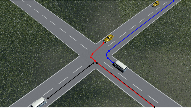
Figure 13: Distributed hierarchical control of autonomous cars along preassigned paths.

Let the trajectories of the $N$ vehicles be defined by cubic spline curves

$$\gamma^{[j]}(s)=\left(\begin{array}[]{c}x^{[j]}(s)\\ y^{[j]}(s)\end{array}\right),\qquad 0\leq s\leq L^{[j]},j=1,\ldots,N,$$

which interpolate given way-points $(x_{i}^{[j]},y_{i}^{[j]})$, $i=0,\ldots,M^{[j]}$, $M^{[j]}\in\mathbb{N}$, i.e.

$$\gamma^{[j]}(s_{i}^{[j]})=\left(\begin{array}[]{c}x_{i}^{[j]}\\ y_{i}^{[j]}\end{array}\right),\qquad i=0,\ldots,M^{[j]},j=1,\ldots,N.$$

Herein, the curves are parametrized with respect to their arc lengths with

$$s^{[j]}_{0}:=0,\quad s^{[j]}_{i+1}:=s^{[j]}_{i}+\sqrt{\left(x^{[j]}_{i+1}-x^{[j]}_{i}\right)^{2}+\left(y^{[j]}_{i+1}-y^{[j]}_{i}\right)^{2}},\quad i=0,\ldots,M^{[j]}-1,$$

and $L^{[j]}:=s_{M^{[j]}}$. The initial value problem

$$(s^{[j]})^{\prime}(t)=v^{[j]}(t),\qquad s^{[j]}(0)=0$$ (35)

describes the motion of the j-th vehicle alongside the spline curve $\gamma^{[j]}$, where $t$ denotes the time and $v^{[j]}(t)$ the velocity of the j-th vehicle at time $t$. We assume that we are able to control the velocity $v^{[j]}(t)\in[v^{[j]}_{min},v^{[j]}_{max}]$ of the vehicle, where $v^{[j]}_{min}$ and $v^{[j]}_{max}$ are the minimum and maximum velocity, respectively. The position of the j-th vehicle at time $t$ is then given by $\gamma^{[j]}(s^{[j]}(t))=(x^{[j]}(s^{[j]}(t)),y^{[j]}(s^{[j]}(t)))^{\top}$.

In Step 2a of the distributed hierarchical model predictive control algorithm, the j-th vehicle has to solve the following optimal control problem on the time horizon $[t_{i},t_{i}+T]$, where $s^{[j]}_{\star}$ denotes the terminal arc-length for vehicle $j$ and $r>0$ is a given security distance. For simplicity we use a ball-shaped constraint for collision avoidance.

Minimize

$$\frac{1}{2}(s^{[j]}(t_{i}+T)-s^{[j]}_{\star})^{2}$$

subject to the constraints

$$(s^{[j]})^{\prime}(t) =v^{[j]}(t), t\in[t_{i},t_{i}+T],$$

$$v^{[j]}(t) \in[v^{[j]}_{min},v^{[j]}_{max}], t\in[t_{i},t_{i}+T],$$

$$\|\gamma^{[j]}(s^{[j]}(t))-\gamma^{[k]}(s^{[k]}(t))\|^{2} \geq r^{2}, \forall k\in I_{PR}(j)(t_{i}),t\in[t_{i},t_{i}+T].$$

Instead of controlling the velocity directly it is also possible to control the acceleration of the vehicles, compare (8), or to introduce a delay as in (9).

4.4 Numerical Results

We present numerical results for the distributed hierarchical model predictive controller in Sections 4.1, 4.2 using the full maneuverability of the cars. For a numerical solution it is important to choose suitable parameters. Especially the selection of the prediction horizon length $T$ and the control horizon length $\tau$ as well as the weights $\alpha_{1},\alpha_{2},\alpha_{3}$ is essential. If the prediction horizon is too short the reaction time might be to brief, if it is too large the computational effort is too high. The computational effort can also be reduced by the choice of the length of the control horizon, but its size also influences the approximation error. The choice of the weights for the controls are linked to the range of the controls and the preferred driving style.

We tested our approach for several everyday scenarios for $N=2$ or $N=3$ cars. All cars are subject to the same car model so they have the same dynamics and the same box-constraints as well as the same limits for velocity and steering angle. We also assumed that the cars are driving in an equal way, i.e. the objective function (33) of each car has the same weights. Furthermore the cars are allowed to occupy the entire road. Since all cars have the same parameters, we suppress the index $j$ throughout and used the following values:

$$\begin{array}[]{lcllcllcl}T&=&2[s]&\qquad\tau&=&0.1[s]&&&\\ \alpha_{1}&=&1&\qquad\alpha_{2}&=&1&\qquad\alpha_{3}&=&10\\ v_{\min}&=&1[m/s]&\qquad v_{\max}&=&10[m/s]&&&\\ a_{\min}&=&-10[m/s^{2}]&\qquad a_{\max}&=&1.5[m/s^{2}]&\qquad w_{\max}&=&0.5[rad]\\ \ell&=&4[m]&\qquad r_{x}&=&3.5[m]&\qquad r_{y}&=&2.5[m]\end{array}$$

Example 3 (Scenario 1: Avoiding a parking car)

In this scenario we consider two consecutive cars which drive in the same lane and direction as shown in Figure 14. The car in the front is going straight for some time and then it parks in the right lane. The second car is driving behind the first car with the same velocity until the car in the front stops. The parked car is then considered to be an obstacle by the second car and an evasive maneuver is executed. After the second car passed by the first car it changes from the left to right lane again.

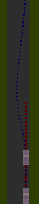
Figure 14: Scenario 1: Trajectory (left) and snapshots of the motion (pictures on the right).

Example 4 (Scenario 2: Two cars driving through a narrow space.)

This time we examine two cars cars which move towards each other from opposite directions and both cars have to pass through a narrow space in the middle of the road as shown in Figure 15. The car coming from below is closer to the obstacle. Therefore it drives through the narrow space first while the second car slows down and waits until the first car passed through the obstacle. Then the second car accelerates and also moves through the narrow space.

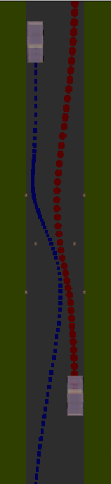
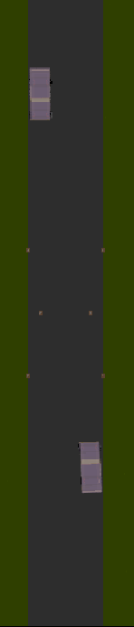
Figure 15: Scenario 2: Trajectory (left) and snapshots of the motion (pictures on the right).

Example 5 (Scenario 3: Three cars at a intersection)

For the last scenario we consider three cars which cross each other at a intersection, compare Figure 16. In this case, traffic rules apply and the cars on the right of each car have higher priority, i.e. the car coming from below has a higher hierarchy level than the car coming from the left, which has a higher priority than the car coming from above, which has to drive onto the left lane of the road so that the car in the middle is able to turn left without collision. The car from below is allowed to ignore the other cars and is able to turn left without collision as shown in figure 17.

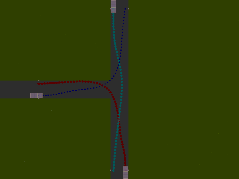
Figure 16: Scenario 3: Trajectories.

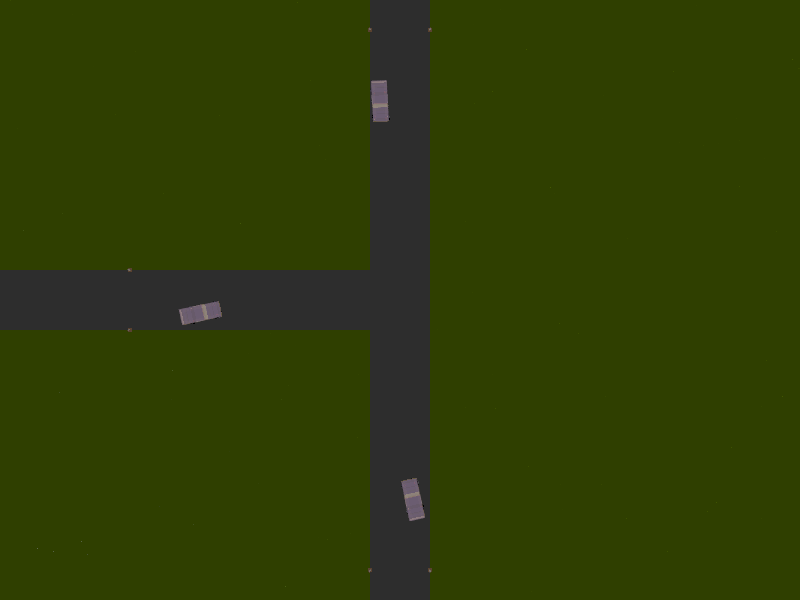
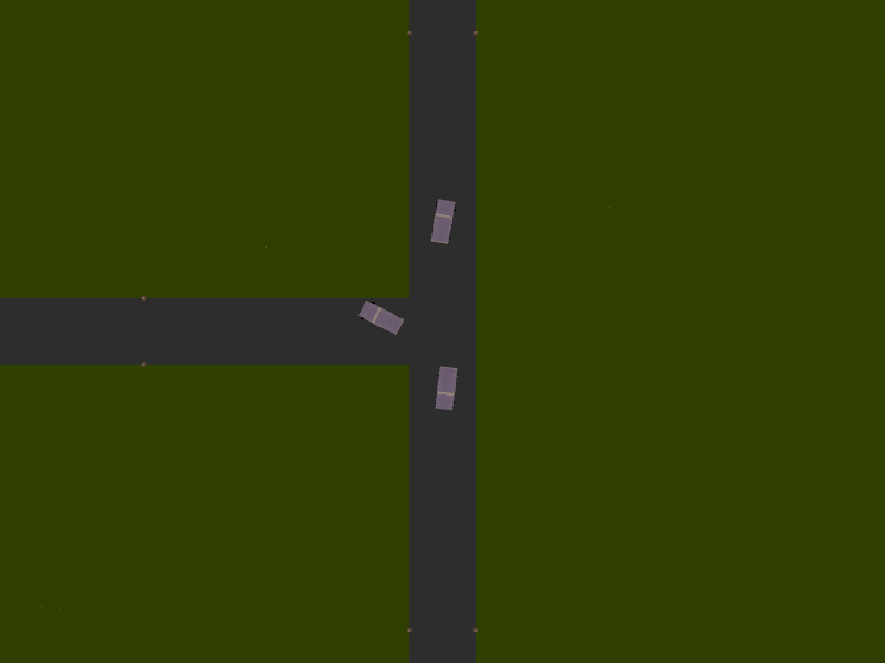
Figure 17: Snapshots of scenario 3.

5 A Tracking Controller for Spline Curves

Once a reference track has been obtained, e.g., by the techniques in Section 3, the task is to follow the track with a real car. To this end let the reference track (=desired track) be given by a cubic spline curve

$$\gamma(t):=\left(\begin{array}[]{c}x_{d}(t)\\ y_{d}(t)\end{array}\right),\qquad t\in[t_{0},t_{f}],$$ (36)

which interpolates the solution obtained by one of the techniques in Section 3 at given grid points within $[t_{0},t_{f}]$. The goal is to design a nonlinear feedback controller according to the flatness concept in Fliess95 ; Rotella2002 ; Martin2003 . The basic idea is to use inverse kinematics in order to find a feedback law for the control inputs of the car. To this end we consider the system of differential equations given by (5)-(7), where we control the velocity $v$ and the steering angle $\delta$. We assume that we can measure the outputs

$$y_{1}:=x\qquad\mbox{and}\qquad y_{2}:=y,$$

i.e. the (x,y)-position of the vehicle. By differentiation we obtain

$$y_{1}^{\prime} = x^{\prime}=v\cos\psi,$$ (37)

$$y_{1}^{\prime\prime} = x^{\prime\prime}=v^{\prime}\cos\psi-v\psi^{\prime}\sin\psi=v^{\prime}\cos\psi-\frac{v^{2}}{\ell}\sin\psi\tan\delta,$$ (38)

$$y_{2}^{\prime} = y^{\prime}=v\sin\psi,$$ (39)

$$y_{2}^{\prime\prime} = y^{\prime\prime}=v^{\prime}\sin\psi+v\psi^{\prime}\cos\psi=v^{\prime}\sin\psi+\frac{v^{2}}{\ell}\cos\psi\tan\delta.$$ (40)

Multiplication of (37) by $\cos\psi$ and of (39) by $\sin\psi$, adding both equations, exploiting $\psi=\arctan(y^{\prime}/x^{\prime})$ and solving for the control $v$ yields

$$v=V(y_{1},y_{2}) := y_{1}^{\prime}\cos\left(\arctan\left(\frac{y_{2}^{\prime}}{y_{1}^{\prime}}\right)\right)+y_{2}^{\prime}\sin\left(\arctan\left(\frac{y_{2}^{\prime}}{y_{1}^{\prime}}\right)\right)$$

$$= \sqrt{(y_{1}^{\prime})^{2}+(y_{2}^{\prime})^{2}}.$$

Likewise, multiplication of (38) by $\sin\psi$ and of (40) by $\cos\psi$, subtracting equations, exploiting $\psi=\arctan(y^{\prime}/x^{\prime})$, $v=\sqrt{(y_{1}^{\prime})^{2}+(y_{2}^{\prime})^{2}}$, and solving for the control $\delta$ yields

$$\delta=\Delta(y_{1},y_{2}) := \arctan\left(\frac{\ell\left(y_{2}^{\prime\prime}\cos\left(\arctan\left(\frac{y_{2}^{\prime}}{y_{1}^{\prime}}\right)\right)-y_{1}^{\prime\prime}\sin\left(\arctan\left(\frac{y_{2}^{\prime}}{y_{1}^{\prime}}\right)\right)\right)}{v^{2}}\right)$$

$$= \arctan\left(\frac{\ell\left(y_{2}^{\prime\prime}y_{1}^{\prime}-y_{1}^{\prime\prime}y_{2}^{\prime}\right)}{\left(\left(y_{1}^{\prime}\right)^{2}+\left(y_{2}^{\prime}\right)^{2}\right)^{\frac{3}{2}}}\right).$$

If we introduce the reference coordinates $x_{d}$ and $y_{d}$ (=desired outputs) from (36) into these formula, then the corresponding controls $v_{d}=V(x_{d},y_{d})$ and $\delta_{d}=\Delta(x_{d},y_{d})$ would track the reference input provided the initial value is consistent with the reference trajectory. However, in practice there will be deviations due to modeling errors or disturbances. Hence, we need a feedback control law that is capable of taking deviations from the reference input into account. Such a feedback control law reads as follows, compare Rotella2002 for general flat systems:

$$K_{v}(y_{1},y_{2},y_{1,d},y_{2,d}):=\sqrt{\left(y_{1,d}^{\prime}-k_{1}\left(y_{1}-y_{1,d}\right)\right)^{2}+\left(y_{2,d}^{\prime}-k_{2}\left(y_{2}-y_{2,d}\right)\right)^{2}},$$

and

$$K_{\delta}(y_{1},y_{2},y_{1,d},y_{2,d}):=$$

$$\qquad\arctan\left(\ell\,\frac{\left(y_{2,d}^{\prime\prime}-k_{5}\left(y_{2}^{\prime}-y_{2,d}^{\prime}\right)-k_{6}\left(y_{2}-y_{2,d}\right)\right)\,y_{1}^{\prime}}{\left(\left(y_{1}^{\prime}\right)^{2}+\left(y_{2}^{\prime}\right)^{2}\right)^{\frac{3}{2}}}\right.$$

$$\qquad\qquad\qquad\left.-\ell\frac{\left(y_{1,d}^{\prime\prime}-k_{3}\left(y_{1}^{\prime}-y_{1,d}^{\prime}\right)-k_{4}\left(y_{1}-y_{1,d}\right)\right)\,y_{2}^{\prime}}{\left(\left(y_{1}^{\prime}\right)^{2}+\left(y_{2}^{\prime}\right)^{2}\right)^{\frac{3}{2}}}\right).$$

Herein, $k_{1},\ldots,k_{6}$ are constants that influence the response time. $y_{1}\ (=x)$ and $y_{2}\ (=y)$ are the actual measurements of the car’s midpoint position of the rear axle and $y_{1,d}\ (=x_{d})$ and $y_{2,d}\ (=y_{d})$ are the reference coordinates, respectively. In addition, the derivatives $y_{1}^{\prime}=x^{\prime}$ and $y_{2}^{\prime}=y^{\prime}$ need to be estimated as well, for instance by finite difference approximations using the position measurements.

If we insert this feedback control law into our system, we obtain the closed loop system

$$x^{\prime}(t) =K_{v}(x(t),y(t),x_{d}(t),y_{d}(t))\cos\psi(t),$$ (41)

$$y^{\prime}(t) =K_{v}(x(t),y(t),x_{d}(t),y_{d}(t))\sin\psi(t),$$ (42)

$$\psi^{\prime}(t) =\frac{K_{v}(x(t),y(t),x_{d}(t),y_{d}(t))}{\ell}\tan K_{\delta}(x(t),y(t),x_{d}(t),y_{d}(t)).$$ (43)

To study the stability behavior we assume $k_{1}=k_{2},k_{3}=k_{5},k_{4}=k_{6}$ and linearize the right side of the system with respect to the reference trajectory, which gives us the time variant matrix

$$A=\begin{pmatrix}-\frac{k_{1}\,\left(x_{d}^{\prime}\right)^{2}}{v_{d}}&-\frac{k_{1}\,x_{d}^{\prime}\,y_{d}^{\prime}}{v_{d}}&-y_{d}^{\prime}\\ -\frac{k_{1}\,x_{d}^{\prime}\,y_{d}^{\prime}}{v_{d}}&-\frac{k_{1}\,\left(y_{d}^{\prime}\right)^{2}}{v_{d}}&x_{d}^{\prime}\\ \frac{k_{1}\,\left(y_{d}^{\prime\prime}\,\left(x_{d}^{\prime}\right)^{2}-x_{d}^{\prime\prime}\,x_{d}^{\prime}\,y_{d}^{\prime}\right)-k_{3}\,y_{d}^{\prime}\,v_{d}^{2}}{v_{d}^{4}}&\frac{k_{1}\left(y_{d}^{\prime\prime}\,x_{d}^{\prime}\,y_{d}^{\prime}-x_{d}^{\prime\prime}\,\left(y_{d}^{\prime}\right)^{2}\right)-k_{3}\,y_{d}^{\prime}\,v_{d}^{2}}{v_{d}^{4}}&-k_{2}\end{pmatrix},$$

with $v_{d}:=\sqrt{\left(x_{d}^{\prime}\right)^{2}+\left(y_{d}^{\prime}\right)^{2}}$, where we suppressed the argument $t$ for notational simplicity. The characteristic polynomial of the matrix is

$$\det(\lambda\,I_{4}-A)=\left(\lambda^{2}+k_{3}\lambda+k_{4}\right)\left(\lambda+k_{1}\right).$$

It follows, if $\lambda+k_{1}$ and $\lambda^{2}+k_{3}\lambda+k_{4}$ are Hurwitz the linearized system is asymptotic stable and thereby the closed loop nonlinear system is locally asymptotic stable.

Measurement errors can be modeled by introducing white noise $(x_{wn},y_{wn})^{\top}$ and $(x^{\prime}_{wn},y^{\prime}_{wn})^{\top}$ into the feedback control law, i.e. by changing $x$ and $y$ to $x-x_{wn}$ and $y-y_{wn}$ and by changing $x^{\prime}$ and $y^{\prime}$ to $x^{\prime}-x^{\prime}_{wn}$ and $y^{\prime}-y^{\prime}_{wn}$.

Example 6 (Tracking controller)

To test the constructed feedback controller we consider to have a constant reference velocity $v_{d}=11.5\,[\frac{m}{s}]$ and $\ell=2.8\,[m]$ to be the distance from rear axle to front axle. For the parameters in the closed loop system we chose $k_{1}=k_{2}=1$, $k_{3}=k_{4}=k_{5}=k_{6}=2$. For the system with white noise we chose a random number generator with values in the interval $[-10,10)$ (in meters) for the $(x,y)$-position and in the interval $[-2,2]$ (in meters per second) for the velocities $(x^{\prime},y^{\prime})$. In practice it is possible to measure the actual position with a tolerance of below one millimeter, but for illustration purposes we use a higher tolerance to test the tracking ability of the controller. For the system with an offset we changed the initial state from $(-26,-1)^{\top}$ to $(-16,9)^{\top}$. In all cases the control values of the feedback control law are projected into the feasible control set $[0,50]$ for the velocity $v$ and to $[-\pi/6,\pi/6]$ for the steering angle $\delta$.

Figure 18 shows the simulations with the feedback controlled system (41) - (43) for a given track at a sampling rate of 20 Hz. For better visibility only every 5th data point is plotted in Figure 18. In all cases the controller is able to accurately follow the track.

Figure 18: Tracking controller output: Trajectory of car with initial position on the track (top), with white noise (middle), and with white noise and initial state offset (bottom).

- (1) Althoff, M.: Reachability analysis and its application to the safety assessment of autonomous cars. Dissertation, Technische Universität München (2010). Http://nbn-resolving.de/urn/resolver.pl?urn:nbn:de:bvb:91-diss-20100715-963752-1-4
- (2) Althoff, M., Krogh, B.H.: Zonotope bundles for the efficient computation of reachable sets. In: Proc. of the 50th IEEE Conference on Decision and Control, pp. 6814–6821 (2011)
- (3) Bertsekas, D.P.: Dynamic programming and optimal control. Vol. 2. 4th ed., 4th ed. edn. Belmont, MA: Athena Scientific (2012)
- (4) Betts, J.T.: Practical methods for optimal control using nonlinear programming, Advances in Design and Control, vol. 3. SIAM, Philadelphia (2001)
- (5) Bock, H.G., Plitt, K.J.: A Multiple Shooting Algorithm for Direct Solution of Optimal Control Problems. Proceedings of the 9th IFAC Worldcongress, Budapest, Hungary (1984)
- (6) Burger, M.: Calculating road input data for vehicle simulation. Multibody System Dynamics pp. 1–18 (2013)
- (7) Burger, M., Speckert, M., Dreßler, K.: Optimal control of multibody systems for the calculation of invariant input loads. In: C.e.a. Schindler (ed.) Proceedings of the 1st Commercial Vehicle Technology Symposium (CVT 2010), pp. 387–396. Shaker Verlag (2010)
- (8) Büskens, C., Maurer, H.: Sensitivity Analysis and Real-Time Optimization of Parametric Nonlinear Programming Problems. In: M. Grötschel, S.O. Krumke, J. Rambau (eds.) Online Optimization of Large Scale Systems, pp. 3–16. Springer (2001)
- (9) Cormen, T. H. and Leiserson, C. E. and Rivest, R. L. and Stein, C.: Introduction to Algorithms, 3 edn. MIT Press (2009)
- (10) Dariana, R., Schmidt, S., Kasper, R.: Optimization based obstacle avoidance. In: World Academie of Science, Engineering and Technology (WASET), 8.2014, 9, pp. 1084–1089 (2014)
- (11) Dariani, R., Schmidt, S., Kasper, R.: Real time optimization path planning strategy for an autonomous vehicle with obstacle avoidance. In: FISITA 2014 World Automotive Congress; 35 (Maastricht) : 2014.06.02-06, Art. F2014-IVC-028 (2014)
- (12) Escande, A., Miossec, S., Benallegue, M., Kheddar, A.: A strictly convex hull for computing proximity distances with continuous gradients. Robotics, IEEE Transactions on 30(3), 666–678 (2014)
- (13) Findeisen, R., Allgöwer, F., Fischer, J., Gross, D., Grüne, L., Hanebeck, U.D., Pannek, J., Stursberg, O., Worthmann, K., Varutti, P., Kern, B., Reble, M., Müller, M.: Distributed and Networked Model Predictive Control. In: J. Lunze (ed.) Control Theory of Digitally Networked Dynamic Systems, pp. 111–167. Springer (2014)
- (14) Fliess, M., Levine, J.L., Martin, P., Rouchon, P.: Flatness and defect of non-linear systems: introductory theory and examples. International Journal of Control 61(6), 1327–1361 (1995)
- (15) Gallrein, A., Baecker, M.: Cdtire: a tire model for comfort and durability applications. Vehicle System Dynamics 45 Supplement, 69–77 (2007)
- (16) Gallrein, A., Baecker, M., Burger, M., Gizatullin, A.: An advanced flexible realtime tire model and its integration into fraunhofer’s driving simulator. Tech. rep., SAE Technical Paper 2014-01-0861 (2014)
- (17) Gerdts, M.: A Moving Horizon Technique for the Simulation of Automobile Test-Drives. ZAMM 83(3), 147–162 (2003)
- (18) Gerdts, M.: Solving Mixed-Integer Optimal Control Problems by Branch&Bound: A Case Study from Automobile Test-Driving with Gear Shift. Optimal Control, Applications and Methods 26(1), 1–18 (2005)
- (19) Gerdts, M.: A variable time transformation method for mixed-integer optimal control problems. Optimal Control, Applications and Methods 27(3), 169–182 (2006)
- (20) Gerdts, M.: Optimal control of ODEs and DAEs. Walter de Gruyter, Berlin/Boston (2012)
- (21) Gerdts, M.: Ocpid-dae1 – optimal control and parameter identification with differential-algebraic equations of index 1. Tech. rep., User’s Guide, Engineering Mathematics, Department of Aerospace Engineering, University of the Federal Armed Forces at Munich, http://www.optimal-control.de (2013)
- (22) Gerdts, M., Henrion, R., Hömberg, D., Landry, C.: Path planning and collision avoidance for robots. Numerical Algebra Control and Optimization 2(3), 437–463 (2012). DOI 10.3934/naco.2012.2.437
- (23) Gerdts, M., Karrenberg, S., Müller-Beßler, B., Stock, G.: Generating locally optimal trajectories for an automatically driven car. Optimization and Engineering 10, 439–463 (2009)
- (24) Geyer, H.R.: Realisierung einer modell-prädiktiven regelung auf modellfahrzeugen (in german; realization of a model-predictive control concept on scale cars). Master’s thesis, University of the Federal Armed Forces at Munich, Institute of Mathematics and Applied Computing, Neubiberg (2014)
- (25) Gilbert, E., Johnson, D.: Distance functions and their application to robot path planning in the presence of obstacle. IEEE Journal of Robotics and Automation RA-1, 21–30 (1985)
- (26) Gilbert, E., Johnson, D., Keerthi, S.: a fast procedure for computing the distance between complex objects in three-dimensional space. IEEE Journal of Robotics and Automation 4(2), 193–203 (1988)
- (27) Groß, D., Stursberg, O.: Distributed predictive control of communicating and constrained systems. ZAMM - Zeitschrift für Angewandte Mathematik und Mechanik 94(4), 303–316 (2014)
- (28) Grüne, L., Pannek, J.: Nonlinear model predictive control. Theory and algorithms. London: Springer (2011)
- (29) Ioffe, A.D., Tihomirov, V.M.: Theory of extremal problems. North-Holland Publishing Company, Amsterdam, New York, Oxford (1979)
- (30) Johnson, D., Gilbert, E.: Minimum time robot path planning in the presence of obstacles. In: Decision and Control, 1985 24th IEEE Conference on, vol. 24, pp. 1748–1753 (1985)
- (31) Kianfar, R., Augusto, B., Ebadighajari, A., Hakeem, U., Nilsson, J., Raza, A., Tabar, R.S., Irukulapati, N.V., Englund, C., Falcone, P., Papanastasiou, S., Svensson, L., Wymeersch, H.: Design and Experimental Validation of a Cooperative Driving System in the Grand Cooperative Driving Challenge. IEEE Transactions on Intelligent Transportation Systems 13(3), 994–1007 (2012)
- (32) Kirches, C., Sager, S., Bock, H., Schlöder, J.: Time-optimal control of automobile test drives with gear shifts. Optimal Control Applications and Methods (2010). DOI http://dx.doi.org/10.1002/oca.892. URL http://mathopt.de/PUBLICATIONS/Kirches2010.pdf. DOI 10.1002/oca.892
- (33) Korte, B., Vygen, J.: Combinatorial Optimization – Theory and Algorithms, Algorithms and Combinatorics, vol. 21, fourth edition edn. Springer Berlin Heidelberg (2008)
- (34) Kurzhanski, A.B., Varaiya, P.: Dynamics and control of trajectory tubes – theory and computation. Systems & Control: Foundations & Applications. Birkhäuser, Springer Cham Heidelberg New York Dordrecht London (2014)
- (35) Martin, P., Murray, R.M., Rouchon, P.: Flat systems, equivalence and trajectory generation. Tech. rep., CDS Technical Report, http://www.cds.caltech.edu/ murray/papers/2003d_mmr03-cds.html (2003)
- (36) Maurer, H., Augustin, D.: Sensitivity Analysis and Real-Time Control of Parametric Optimal Control Problems Using Boundary Value Methods. In: M. Grötschel, S.O. Krumke, J. Rambau (eds.) Online Optimization of Large Scale Systems, pp. 17–55. Springer (2001)
- (37) Maurer, M. and Gerdes, J. C. and Lenz, B. and Winner, H.: Autonomes Fahren – Technische, rechtliche und gesellschaftliche Aspekte. Springer Vieweg, Berlin Heidelberg (2015)
- (38) Nachtigal, H.: Berechnung von starttrajektorien zur optimierung von virtuellen testfahrten mit hindernissen (in german; computation of initial trajectories for optimized virtual testdrives in the presence of obstacles). Tech. rep., University of the Federal Armed Forces at Munich, Institute of Mathematics and Applied Computing, Bachelor thesis, Neubiberg (2015)
- (39) Nilsson, J., Fredriksson, J., , Odblom, A.C.: Verification of collision avoidance systems using reachability analysis. In: Proceedings of 19th IFAC World Congress, pp. 10,676––10,681 (2014)
- (40) Palma, V.G.: Robust updated mpc schemes. Ph.D. thesis, Universität Bayreuth, Bayreuth (2015)
- (41) Pannek, J.: Parallelizing a state exchange strategy for noncooperative distributed nmpc. System & Control Letters 62, 29–36 (2013)
- (42) Papadimitriou, C.H., Steiglitz, K.: Combinatorial Optimization–Algorithms and Complexity. Dover Publications (1998)
- (43) Polak, E.: An historical survey of computational methods in optimal control. SIAM Review 15(2), 553–584 (1973)
- (44) Rill, G.: Road Vehicle Dynamics – Fundamentals and Modeling. Taylor & Francis (2011)
- (45) Rotella, F., Carrillo, F.J., Ayadi, M.: Polynomial controller design based on flatness. Kybernetika 38(5), 571–584 (2002)
- (46) Schmidt, S., Dariana, R., Kasper, R.: Real-time path planning for an autonomous vehicle using optimal control. In: OPT-i. - Kos Island, insges. 10 S., 2014 ; Kongress: OPT-i; (Kos, Island, Greece) : 2014.06.04-06 (2014)
- (47) Wood, T., Esfahani, P.M., Lygeros, J.: Hybrid Modelling and Reachability on Autonomous RC-Cars. In: IFAC Conference on Analysis and Design of Hybrid Systems (ADHS). Eindhoven, Netherlands (2012). URL http://control.ee.ethz.ch/index.cgi?page=publications;action=%details;id=4040
- (48) Xausa, I.: Verification of collision avoidance systems using optimal control and sensitivity analysis. Ph.D. thesis, University of the Federal Armed Forces at Munich, Neubiberg (2015)