The Hybrid Bootstrap: A Drop-in Replacement for Dropout

Abstract

Regularization is an important component of predictive model building. The hybrid bootstrap is a regularization technique that functions similarly to dropout except that features are resampled from other training points rather than replaced with zeros. We show that the hybrid bootstrap offers superior performance to dropout. We also present a sampling based technique to simplify hyperparameter choice. Next, we provide an alternative sampling technique for convolutional neural networks. Finally, we demonstrate the efficacy of the hybrid bootstrap on non-image tasks using tree-based models. The code used to generate this paper is available here.

1 Introduction

The field of machine learning offers many potent models for inference. Unfortunately, simply optimizing how well these models perform on a fixed training sample often leads to relatively poor performance on new test data compared to models that fit the training data less well. Regularization schemes are used to constrain the fitted model to improve performance on new data.

One popular regularization tactic is to corrupt the training data with independently sampled noise. This constrains the model to work on data that is different from the original training data in a way that does not change the correct inference. Sietsma and Dow demonstrated that adding Gaussian noise to the inputs improved the generalization of neural networks [1]. More recently, Srivastava et al. showed that setting a random collection of layer inputs of a neural network to zero for each training example greatly improved model test performance [2].

Both of these types of stochastic regularization have been shown to be roughly interpretable as types of weight penalization, similar to traditional statistical shrinkage techniques. Bishop showed that using a small amount of additive noise is approximately a form of generalized Tikhonov regularization [3]. Van der Maaten et al. showed that dropout and several other types of sampled noise can be replaced in linear models with modified loss functions that have the same effect [4]. Similarly, Wager et al. showed that, for generalized linear models, using dropout is approximately equivalent to an $l^{2}$ penalty following a scaling of the design matrix [5].

As noted by Goodfellow et al., corrupting noise can be viewed as a form of dataset augmentation [6]. Traditional data augmentation seeks to transform training points in ways that may drastically alter the point but minimally change the correct inference. Corruption generally makes the correct inference more ambiguous. Often, effective data augmentation requires domain-specific knowledge. However, data augmentation also tends to be much more effective than corruption, presumably because it prepares models for data similar to that which they may actually encounter. For example, DropConnect is a stochastic corruption method that is similar to dropout except that it randomly sets neural network weights, rather than inputs, to zero. Wan et al. showed that DropConnect (and dropout) could be used to reduce the error of a neural network on the MNIST [7] digits benchmark by roughly 20 percent. However, using only traditional augmentation they were able to reduce the error by roughly 70 percent [8]. Since corruption seems to be a less effective regularizer than traditional data augmentation, we improved dropout by modifying it to be more closely related to the underlying data generation process.

1.1 The Hybrid Bootstrap

An obvious criticism of dropout as a data augmentation scheme is that one does not usually expect to encounter randomly zeroed features in real data, except perhaps in the “nightmare at test time” [9] scenario where important features are actually anticipated to be missing. One therefore may wish to replace some of the elements of a training point with values more plausible than zeros. A natural solution is to sample a replacement from the other training points. This guarantees that the replacement arises from the correct joint distribution of the elements being replaced. We call this scheme the hybrid bootstrap because it produces hybrids of the training points by bootstrap [10] sampling. More formally, define $\boldsymbol{x}$ to be a vectorized training point. Then a dropout sample point $\tilde{\boldsymbol{x}}$ of $\boldsymbol{x}$ is

$$\tilde{\boldsymbol{x}}=\frac{1}{1-p}\boldsymbol{x}\odot\boldsymbol{\epsilon},$$ (1)

where $\odot$ is the elementwise product, $\boldsymbol{\epsilon}$ is a random vector of appropriate dimension such that $\epsilon_{i}\sim Ber(1-p)$, and $p\in[0,1]$. The normalization by $\frac{1}{1-p}$ seems to be in common use, although it was not part of the original dropout specification [2]. We then define a hybrid bootstrap sample point $\boldsymbol{\overset{\overset{\large.}{\cup}}{x}}$ as

$$\boldsymbol{\overset{\overset{\large.}{\cup}}{x}}=\boldsymbol{x}\odot\boldsymbol{\epsilon}+\boldsymbol{\overset{\large.}{\cup}}\odot(\boldsymbol{1}-\boldsymbol{\epsilon}),$$ (2)

where $\boldsymbol{\overset{\large.}{\cup}}$ is a vectorized random training point and $\boldsymbol{1}$ is a vector of ones of appropriate length. In Figure 1, we compare dropout and hybrid bootstrap sample points for a digit 5.

Figure 1: Dropout randomly (with probability $p$) sets a selection of covariates to zero. The hybrid bootstrap randomly replaces a selection of covariates with those from another training point. The dropout samples in this figure have not been normalized for their corruption levels as would typically be done when used for training.

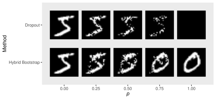
Typically dropout is performed with the normalization given in Equation 1, but we do not use that normalization for this figure because it would make the lightly corrupted images dim; we do use the normalization elsewhere for dropout. This normalization does not seem to be useful for the hybrid bootstrap. One clear difference between the hybrid bootstrap and dropout for the image data of Figure 1 is that the dropout corrupted sample point remains recognizable even for corruption levels greater than 0.5, whereas the hybrid bootstrap sample, unsurprisingly, appears to be more strongly the corrupting digit 0 at such levels. In general, we find that lower fractions of covariates should be resampled for the hybrid bootstrap than should be dropped in dropout.

1.2 Paper outline

In this paper, we focus on applying the hybrid bootstrap to image classification using convolutional neural networks (CNNs) [11] in the same layerwise way dropout is typically incorporated. The basic hybrid bootstrap is an effective tool in its own right, but we have also developed several refinements that improve its performance both for general prediction purposes and particularly for image classification. In Section 3, we discuss a technique for simplifying the choice of the hyperparameter $p$ for the hybrid bootstrap and dropout. In Section 4, we introduce a sampling modification that improves the performance of the hybrid bootstrap when used with convolutional neural networks. In Section 5, we compare the performance of the hybrid bootstrap and dropout for different amounts of training data. Section 6 contains results on several standard benchmark image datasets. The hybrid bootstrap is a useful addition to models besides convolutional neural networks; we present some performance results for the multilayer perceptron [12] and gradient boosted trees [13] in Section 7.

2 CNN Implementation Details

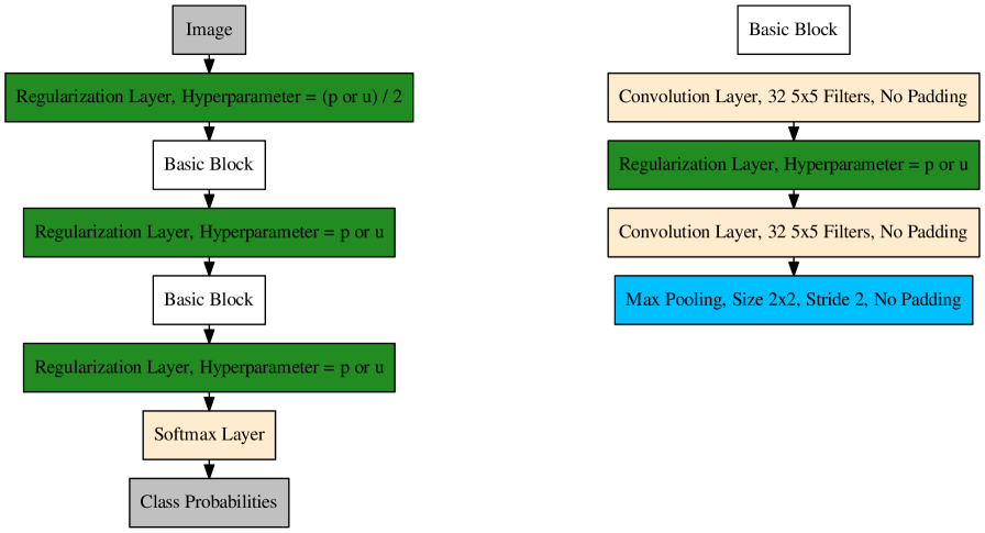
We fit the CNNs in this paper using backpropagation and stochastic gradient descent (SGD) with momentum. The hybrid bootstrap requires selection of $\boldsymbol{\overset{\large.}{\cup}}$ in Equation 2 for each training example. We find that using a $\boldsymbol{\overset{\large.}{\cup}}$ corresponding to the same training point to regularize every layer of a neural network leads to worse performance than using different points for each layer. We use a shifted version of each training minibatch to serve as the collection of $\boldsymbol{\overset{\large.}{\cup}}$ required to compute the input to each layer. We increment the shift by one for each layer. In other words, the corrupting noise for the first element of a minibatch will come from the second element for the input layer, from the third element for the second layer, and so on. We use a simple network architecture given in Figure 2 for all CNN examples except those in Section 6. All activation functions except for the last layer are rectified linear units (ReLUs) [14]. As Srivastava et al. [2] found for dropout, we find that using large amounts of momentum is helpful for obtaining peak performance with the hybrid bootstrap and generally use a momentum of 0.99 by the end of our training schedules, except in Section 6. We make extensive use of both Keras [15], and Theano [16] to implement neural networks and train them on graphics processing units (GPUs).

Figure 2: Network architecture for CNN experiments in this paper (except the benchmark results).

3 Choosing $p$

The basic hybrid bootstrap requires selection of a hyperparameter $p$ to determine what fraction of inputs are to be resampled. This is a nuisance because the quality of the selection can have a dramatic effect on performance, and a lot of computational resources are required to perform cross validation for complicated networks. Fortunately, $p$ need not be a fixed value, and we find that sampling $p$ for each hybrid bootstrap sample to be effective. We sample from a $\text{Uniform}(0,u)$ distribution. Sampling in this way offers two advantages relative to using a single value:

1. Performance is much less sensitive to the choice of $u$ than it is to the choice of $p$ (i.e. tuning is easier).

2. Occasionally employing near-zero levels of corruption ensures that the model performs well on the real training data.

Figure 3: Test set performance (top) and test set performance over the course of training (bottom) using a constant hyperparameter vs. a sampled hyperparameter for dropout and the hybrid bootstrap on the MNIST digits with 1,000 training examples. The colored lines in the bottom panel correspond to the regularization levels indicated in the top panel. Sampled hyperparameters perform as well as constant hyperparameters but are much less sensitive to the choice of $u$ than to $p$.

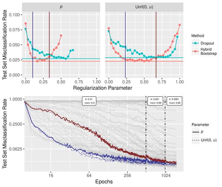
The first advantage is illustrated in the top panel of Figure 3. Clearly there are many satisfactory choices of $u$ for both the hybrid bootstrap and dropout, whereas only a narrow range of $p$ is nearly optimal. However, as the bottom panel of Figure 3 demonstrates, this insensitivity is somewhat contingent upon training for a sufficient number of epochs. The advantages of sampling a regularization level for each training point follow from the way neural networks are fit. SGD and SGD with momentum update the parameters of a neural network by translating them in the direction of the negative gradient of a minibatch or a moving average of the negative gradient of minibatches respectively. The minibatch gradient can be written as

$$\frac{1}{m}\nabla_{\boldsymbol{\theta}}\sum_{i=1}^{m}L(f(\boldsymbol{x}^{(i)};\boldsymbol{\theta}),\boldsymbol{y}^{(i)}),$$ (3)

where $m$ is the number of points in the batch, $\boldsymbol{\theta}$ is the vector of model parameters, $L$ is the loss, $f$ is the model, $\boldsymbol{x}^{(i)}$ is the ith training example in the batch, and $\boldsymbol{y}^{(i)}$ is the target of the ith training example in the batch [6]. Equation 3 can be rewritten using the chain rule as

$$\frac{1}{m}\sum_{i=1}^{m}\left[\nabla_{f(\boldsymbol{x}^{(i)};\boldsymbol{\theta})}L(f(\boldsymbol{x}^{(i)};\boldsymbol{\theta}),\boldsymbol{y}^{(i)})\cdot\frac{Df(\boldsymbol{x}^{(i)};\boldsymbol{\theta})}{d\boldsymbol{\theta}}\right].$$ (4)

The gradient of the loss in Equation 4 is “small” when the loss is small; therefore, the individual contribution to the minibatch gradient is small from individual training examples with small losses. As training progresses, the model tends to have relatively small losses for relatively less-corrupted training points. Therefore, less-corrupted examples contribute less to the gradient after many epochs of training. We illustrate this in Figure 4 by observing the Euclidean norm of the gradient in each layer as training of our experimental architecture on 1,000 MNIST training digits progresses.

Figure 4: As training progresses, training points that have been corrupted less have smaller gradients than more heavily corrupted points.

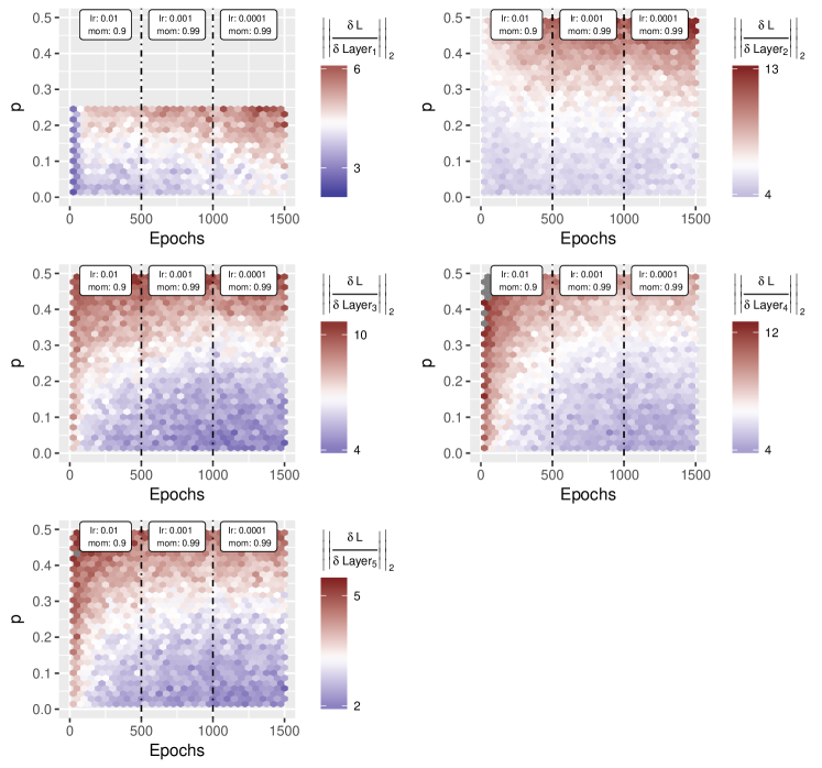
Clearly low probabilities of resampling are associated with smaller gradients. This relationship is somewhat less obvious for layers far from the output because the gradient size is affected by the amount of corruption between these layers and the output.

We have no reason to suppose that the uniform distribution is optimal for sampling the hyperparameter $p$. We employ it because:

1. We can easily ensure that $p$ is between zero and one.

2. Uniformly distributed random numbers are readily available in most software packages.

3. Using the uniform distribution ensures that values of $p$ near zero are relatively probable compared to some symmetric, hump-shaped alternatives. This is a hedge to ensure regularized networks do not perform much worse than unregularized networks. For instance, using the uniform distribution helps assure that the optimization can “get started,” whereas heavily corrupted networks can sometimes fail to improve at all.

There are other plausible substitutes, such as the Beta distribution, which we have not investigated.

4 Structured Sampling for Convolutional Networks

The hybrid bootstrap of Equation 2 does not account for the spatial structure exploited by CNNs, so we investigated whether changing the sampling pattern based on this structure would improve the hybrid bootstrap’s performance on image tasks.

Figure 5: Visualization of different hybrid bootstrap sampling schemes for CNNs.

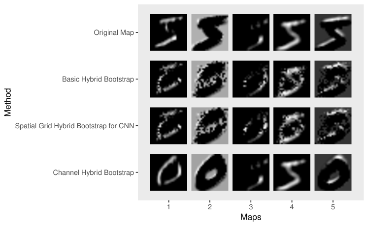
In particular, we wondered if CNNs would develop redundant filters to “solve” the problem of the hybrid bootstrap since the resampling locations are chosen independently for each filter. We therefore considered using the same spatial swapping pattern for every filter, which we call the spatial grid hybrid bootstrap since pixel positions are either swapped or not. Tompson et. al considered dropping whole filters as a modified form of dropout that they call SpatialDropout (their justification is also spatial) [17]. This approach seems a little extreme in the case of the hybrid bootstrap because the whole feature map would be swapped, but perhaps it could work since the majority of feature maps will still be associated with the target class. We call this variant the channel hybrid bootstrap to avoid confusion with the spatial grid hybrid bootstrap.

The feature maps following regularization corresponding to these schemes are visualized in Figure 5. It is difficult to visually distinguish the spatial grid hybrid bootstrap from the basic hybrid bootstrap even though the feature maps for the spatial grid hybrid bootstrap are all swapped at the same locations, whereas the locations for the basic hybrid bootstrap are independently chosen. This may explain their similar performance.

We compare the error rates of the three hybrid bootstrap schemes in the top left panel of Figure 6 for various values of $u$ by training on 1,000 points and computing the accuracy on the remaining 59,000 points in the conventional training set. Both the spatial grid and the channel hybrid bootstrap outperform the basic hybrid bootstrap for low levels of corruption. As $u$ increases, the basic hybrid bootstrap and the spatial grid hybrid bootstrap reach similar levels of performance. Both methods reach a (satisfyingly flat) peak at approximately $u=0.45$. As indicated in the top right panel of Figure 6, the test accuracies of both the basic hybrid bootstrap and the spatial grid hybrid bootstrap are similar for different initializations of the network at this chosen parameter. We compare the redundancy of networks regularized using the three hybrid bootstrap variants at this level of corruption.

One possible measure of the redundancy of filters in a particular layer of a CNN is the average absolute correlation between the output of the filters. We consider the median absolute correlation for 10 different initializations in the bottom panel of Figure 6. The middle two layers exhibit the pattern we expected: the spatial grid hybrid bootstrap leads to relatively small correlations between filters. However, this pattern does not hold for the first and last convolutional layer. If we attempt to reduce the initial absolute correlations of the filters with a rotation, even this pattern does not hold up.

Figure 6: Validation accuracy of structured sampling schemes using 1,000 training images (top left), test accuracy of structured sampling schemes for 10 different initializations (top right), and median absolute correlations of neurons in convolutional layers following training for 10 initializations (bottom).

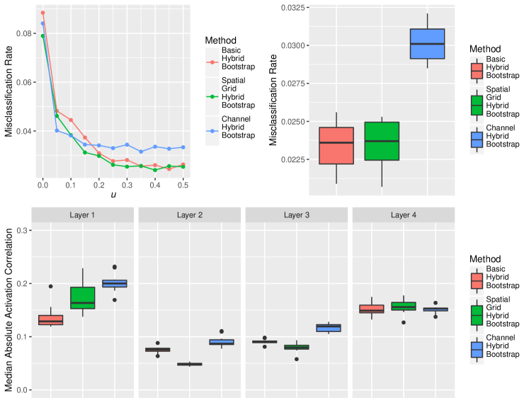
Overall, the difference in performance between the spatial grid hybrid bootstrap and the basic hybrid bootstrap is modest, particularly near their optimal parameter value. We use the spatial grid hybrid bootstrap for CNNs on the basis that it seems to perform at least as well as the basic hybrid bootstrap, and outperforms the basic hybrid bootstrap if we select a $u$ that is too small.

5 Performance as a Function of Number of Training Examples

We find the hybrid bootstrap to be particularly effective when only a small number of training points are available. In the most extreme case, only one training point per class exists. So-called one-shot learning seeks to discriminate based on a single training example. In Figure 7, we compare the performance of dropout and the hybrid bootstrap for different training set sizes using the hyperparameters $u=0.45$ and $u=0.65$ for the hybrid bootstrap and dropout respectively.

Figure 7: Performance of the hybrid bootstrap compared to dropout for different training set sizes. Here a random guess assigns a probability of $\frac{1}{k}$ where $k$ is the number of classes.

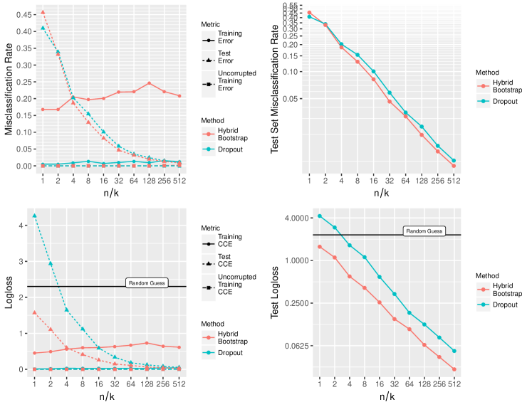
Both techniques perform remarkably well even for small dataset sizes but the hybrid bootstrap has a clear advantage. If one considers the logloss as a measure of model performance, the hybrid bootstrap works even when only one or two examples from each class are available. However, dropout is less effective than assigning equal odds to each class for those dataset sizes. The error rate of the network on dropout-corrupted data (shown in the top left panel of Figure 7) is quite low even though there is a large amount of dropout. This comparison is potentially unfair to dropout as an experienced practitioner may suspect that our test architecture contains too many parameters for such a small training set before using it. However, for the less-experienced who must rely on it, cross validation is challenging with only one training point.

6 Benchmarks

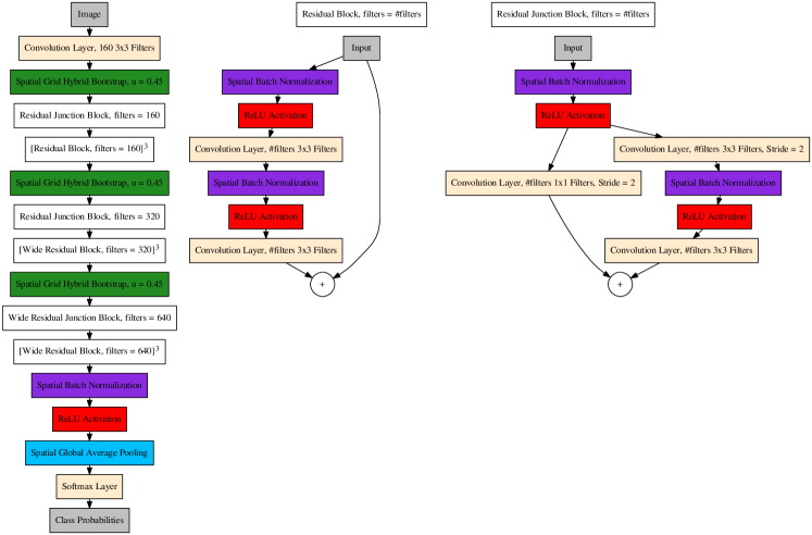
The previous sections employed smaller versions of the MNIST training digits for the sake of speed, but clearly the hybrid bootstrap is only useful if it works for larger datasets and for data besides the MNIST digits. To evaluate the hybrid bootstrap’s performance on three standard image benchmarks, we adopt a CNN architecture very similar to the wide residual networks (WRNs) of Zagoruyko and Komodakis [18] with three major differences. First, they applied dropout immediately prior to certain weight layers. Since their network uses skip connections, this means difficult regularization patterns can be bypassed, defeating the regularization. We therefore apply the hybrid bootstrap prior to each set of network blocks at a particular resolution. Second, we use 160 rather than 16 filters in the initial convolutional layer. This allows us to use the same level of hybrid bootstrap for each of the three regularization layers. Third, their training schedule halted after decreasing the learning rate three times by 80%. Our version of the network continues to improve significantly at lower learning rates, so we decrease by the same amount five times. Our architecture is visualized in Figure 8.

Figure 8: Network architecture for benchmark results. Biases are not used. All convolutional layers have linear activations. Exponents represent the number of repeated layers.

We test this network on the CIFAR10 and CIFAR100 datasets, which consist of RGB images with 50,000 training examples and 10,000 test cases each and 10 and 100 classes respectively [19]. We also evaluate this network on the MNIST digits. We augment the CIFAR data with 15% translations and horizontal flips. We do not use data augmentation for the MNIST digits. The images are preprocessed by centering and scaling according to the channel-wise mean and standard deviation of the training data. We use SGD with Nesterov momentum 0.9 and start with learning rate 0.1. The learning rate is decreased by 80% every 60 epochs and the network is trained for 360 epochs total. The results are given in Table 1. We attempted to use dropout in the same position as we use the hybrid bootstrap, but this worked very poorly. At dropout levels $p=0.5$ and $p=0.25$, the misclassification rates on the CIFAR100 test set are 50.56% and 28.83% respectively, which is much worse than the hybrid bootstrap result. To have a real comparison to dropout, we have included the dropout-based results from the original wide residual network paper. It is apparent in Table 1 that adding the hybrid bootstrap in our location makes a much bigger difference than adding dropout to the residual blocks.

Table 1: Benchmark results. Values are misclassification percentages. The CIFAR datasets are augmented with translations and flips. The MNIST digits are not augmented.

Dataset	Hybrid Bootstrap	No Stochastic Reg.	Dropout	No Stochastic Reg.
	(Our Architecture)	(Our Architecture)	(WRN 28-10)	(WRN 28-10)
CIFAR10	3.4	4.13	3.89	4.00
CIFAR100	18.36	20.1	18.85	19.25
MNIST	0.3	0.66	NA	NA

7 Other Algorithms

The hybrid bootstrap is not only useful for CNNs. It is also applicable to other inferential algorithms and can be applied without modifying their underlying code by expanding the training set in the manner of traditional data augmentation.

7.1 Multilayer Perceptron

The multilayer perceptron is not of tremendous modern interest for image classification, but it is still an effective model for other tasks. Dropout is commonly used to regularize the multilayer perceptron, but the hybrid bootstrap is even more effective. As an example, we train a multilayer perceptron on the MNIST digits with 2 “hidden” layers of $2^{13}$ neurons each with ReLU activations and $u=0.225$, $u=0.45$ hybrid bootstrap regularization for each layer respectively. We use weight decay 0.00001 and SGD with momentum 0.9 and batch size 512. We start the learning rate at 0.1 and multiply it by 0.2 every 250 epochs for 1,000 epochs total training. The resulting network has error 0.81% on the MNIST test set. Srivastava et al. used dropout on the same architecture with resulting error 0.95% [2]. However, their training schedule was different and they used a max-norm constraint rather than weight decay. To verify that this improvement is not simply a consequence of these differences rather than the result of replacing dropout with the hybrid bootstrap, we use the same parameters but replace the hybrid bootstrap with dropout $p=0.25$, $p=0.5$ respectively. The resulting network has test set error 1.06%.

7.2 Boosted Trees

One of the most effective classes of prediction algorithms is that based on gradient boosted trees described by Friedman [13]. Boosted tree algorithms are not very competitive with CNNs on image classification problems, but they are remarkably effective for prediction problems in general and have the same need for regularization as other nonparametric models. We use XGBoost [20], a popular implementation of gradient boosted trees.

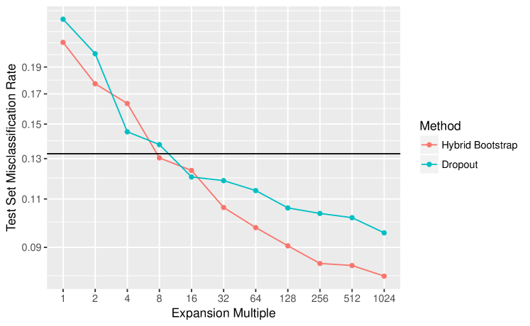
Vinayak and Gilad-Bachrach proposed dropping the constituent models of the booster during training, similar to dropout [21]. This requires modifying the underlying model fitting, which we have not attempted with the hybrid bootstrap. However, if we naively generate hybrid bootstrap data on 1,000 MNIST digits with the hyperparameters $u=0.45$ and $u=0.65$ for the hybrid bootstrap and dropout respectively, we can see that the hybrid bootstrap outperforms dropout in Figure 9. We note that extreme expansion of the training data by hybrid bootstrap sampling seems to be important for peak predictive performance. However, this must be balanced by consideration of the computational cost.

Figure 9: Comparison of boosted tree test set performance on the MNIST digits for stochastic expansions of 1,000 training images. The horizontal line is the performance of an XGBoost model using four times as many trees and a smaller step size, but no additional regularization.

Figure 10: Comparison of different regularization mechanisms for boosted trees for breast cancer malignancy (top) and Titanic passenger survival (bottom). The number of trees selected using cross validation is printed at the top of each panel. Horizontal lines are at the minimum of each curve to aid comparison, but the variation of each curve is of significant importance too.

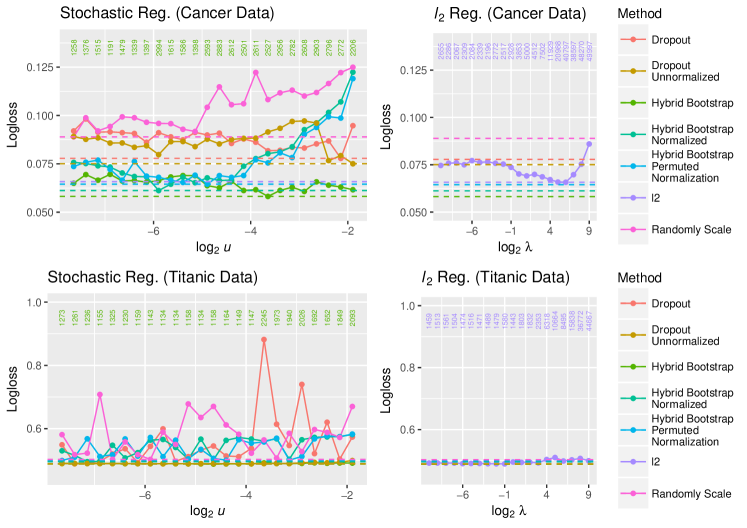
We also compare dropout and the hybrid bootstrap for the breast cancer dataset where malignancy is predicted from a set of 30 features [22]. XGBoost provides its own $l^{2}$-type regularization technique that we typically set to a negligible level when using the hybrid bootstrap. We compare XGBoost‘s $l^{2}$ regularization with several stochastic methods. The stochastic methods are: the hybrid bootstrap, dropout, the hybrid bootstrap with the dropout normalization, the hybrid bootstrap with a random permutation of the dropout normalization, dropout without the normalization, and just the dropout normalization. We expand the training dataset by a factor of 1,000 for the stochastic methods. Early experiments on depth-one trees indicated that simply randomly scaling the data was effective but this does not seem to apply to other tree depths. We randomly split the 569 observations into a training set and a test set and use the median of a five-fold cross validation to select the appropriate number of depth-two trees. We allow at most 50,000 trees for the $l^{2}$ regularized method and 3,000 trees for the stochastic regularization methods. We perform the same the same procedure for the well-known Titanic survival data [23] except the test set is chosen to be the canonical test set. We use only numeric predictors and factor levels with three or fewer levels for the Titanic data, leaving us with $p=7$ and 891 and 418 observations in the training and test sets respectively. The results are given in Figure 10. The hybrid bootstrap outperforms the $l^{2}$ regularization in both cases (very marginally in the case of the Titanic data). The normalized stochastic methods do not seem to be terribly effective, particularly for the Titanic data. We suspect this is because they replace the the factor data with non-factor values. We note that training using the augmented data takes much longer than the $l^{2}$ regularization. However, the number of trees selected for the $l^{2}$ regularization method (printed in the same figure) may be significantly larger than for the stochastic methods, so the stochastic regularizers may offer a computational advantage at inference time. The sizes of these datasets are small, and we note that the $l^{2}$ regularization has a lower (oracle) classification error for the cancer data. Of course, nothing prevents one from using both regularization schemes as part of an ensemble, which works well in our experience.

8 Discussion

The hybrid bootstrap is an effective form of regularization. It can be applied in the same fashion as the tremendously popular dropout technique but offers superior performance. The hybrid bootstrap can easily be incorporated into other existing algorithms. Simply construct hybrid bootstrap data as we do in Section 7. Unlike other noising schemes, the hybrid bootstrap does not change the support of the data. However, the hybrid bootstrap does have some disadvantages. The hybrid bootstrap requires the choice of at least one additional hyperparameter. We have attempted to mitigate this disadvantage by sampling the hybrid bootstrap level, which makes performance less sensitive to the hyperparameter. The hybrid bootstrap performs best when the original dataset is greatly expanded. The magnitude of this disadvantage depends on the scenario in which supervised learning is being used. We think that any case where dropout is being used is a good opportunity to use the hybrid bootstrap. However, there are some cases, such as linear regression, where the hybrid bootstrap seems to offer roughly the same predictive performance as existing methods, such as ridge regression, but at a much higher computational cost. The hybrid bootstrap’s performance may depend on the basis in which the data are presented. This disadvantage is common to many algorithms. One reason we think the hybrid bootstrap works so well for neural networks is that they can create features in a new basis at each layer that can themselves be hybrid bootstrapped, so the initial basis is not as important as it may be for other algorithms.

We have given many examples of the hybrid bootstrap working, but have devoted little attention to explaining why it works. There is a close relationship between hypothesis testing and regularization. For instance, the limiting behavior of ridge regression is to drive regression coefficients to zero, a state which is a common null hypothesis. The limiting behavior of the hybrid bootstrap is to make the class (or continuous target) statistically independent of the regressors, as in a permutation test. Perhaps the hybrid bootstrap forces models to possess a weaker dependence between predictor variables and the quantity being predicted than they otherwise would. We recognize this is a vague explanation (and could be said of other forms of regularization), but we do find that the hybrid bootstrap has a lot of practical utility.

9 Miscellaneous Acknowledgments

While we were writing this paper, Michael Jahrer independently used the basic hybrid bootstrap as input noise (under the alias “swap noise”) for denoising autoencoders as a component of his winning submission to the Porto Seguro Safe Driver Prediction Kaggle competition. Clearly this further establishes the utility of the hybrid bootstrap!

We have also recently learned that there are currently at least three distinct groups that have papers at various points in the publishing process concerning convex combinations of training points, which are similar to hybrid bootstrap combinations [24, 25, 26].

Glossary

CNN

convolutional neural network

GPU

graphics processing unit

ReLU

rectified linear unit

SGD

stochastic gradient descent

WRN

wide residual network

References

- [1] Jocelyn Sietsma and Robert JF Dow. Creating artificial neural networks that generalize. Neural Networks, 4(1):67–79, 1991.
- [2] Nitish Srivastava, Geoffrey E Hinton, Alex Krizhevsky, Ilya Sutskever, and Ruslan Salakhutdinov. Dropout: a simple way to prevent neural networks from overfitting. Journal of Machine Learning Research, 15(1):1929–1958, 2014.
- [3] Chris M Bishop. Training with noise is equivalent to Tikhonov regularization. Neural Computation, 7(1):108–116, 1995.
- [4] Laurens Van Der Maaten, Minmin Chen, Stephen Tyree, and Kilian Q Weinberger. Learning with marginalized corrupted features. In Proceedings of the 30th International Conference on Machine Learning, pages 410–418, 2013.
- [5] Stefan Wager, Sida Wang, and Percy S Liang. Dropout training as adaptive regularization. In Advances in Neural Information Processing Systems, pages 351–359, 2013.
- [6] Ian Goodfellow, Yoshua Bengio, and Aaron Courville. Deep Learning. MIT Press, 2016.
- [7] Yann LeCun, Léon Bottou, Yoshua Bengio, and Patrick Haffner. Gradient-based learning applied to document recognition. Proceedings of the IEEE, 86(11):2278–2324, 1998.
- [8] Li Wan, Matthew Zeiler, Sixin Zhang, Yann L Cun, and Rob Fergus. Regularization of neural networks using DropConnect. In Proceedings of the 30th International Conference on Machine Learning, pages 1058–1066, 2013.
- [9] Amir Globerson and Sam Roweis. Nightmare at test time: robust learning by feature deletion. In Proceedings of the 23rd International Conference on Machine Learning, pages 353–360. ACM, 2006.
- [10] Bradley Efron and Robert J Tibshirani. An Introduction to the Bootstrap. CRC press, 1994.
- [11] Yann LeCun, Bernhard Boser, John S Denker, Donnie Henderson, Richard E Howard, Wayne Hubbard, and Lawrence D Jackel. Backpropagation applied to handwritten zip code recognition. Neural Computation, 1(4):541–551, 1989.
- [12] Frank Rosenblatt. Principles of neurodynamics. perceptrons and the theory of brain mechanisms. Technical report, DTIC Document, 1961.
- [13] Jerome H Friedman. Greedy function approximation: a gradient boosting machine. Annals of statistics, pages 1189–1232, 2001.
- [14] Vinod Nair and Geoffrey E Hinton. Rectified linear units improve restricted Boltzmann machines. In Proceedings of the 27th International Conference on Machine Learning (ICML-10), pages 807–814, 2010.
- [15] François Chollet et al. Keras. https://github.com/fchollet/keras, 2015.
- [16] Theano Development Team. Theano: A Python framework for fast computation of mathematical expressions. arXiv e-prints, abs/1605.02688, May 2016.
- [17] Jonathan Tompson, Ross Goroshin, Arjun Jain, Yann LeCun, and Christoph Bregler. Efficient object localization using convolutional networks. In Proceedings of the IEEE Conference on Computer Vision and Pattern Recognition, pages 648–656, 2015.
- [18] Sergey Zagoruyko and Nikos Komodakis. Wide residual networks. In BMVC, 2016.
- [19] Alex Krizhevsky and Geoffrey Hinton. Learning multiple layers of features from tiny images. Technical report, University of Toronto, 2009.
- [20] Tianqi Chen and Carlos Guestrin. XGBoost: A scalable tree boosting system. In Proceedings of the 22nd ACM SIGKDD International Conference on Knowledge Discovery and Data Mining, pages 785–794. ACM, 2016.
- [21] Rashmi Korlakai Vinayak and Ran Gilad-Bachrach. DART: Dropouts meet Multiple Additive Regression Trees. In Proceedings of the Eighteenth International Conference on Artificial Intelligence and Statistics, pages 489–497, 2015.
- [22] W Nick Street, William H Wolberg, and Olvi L Mangasarian. Nuclear feature extraction for breast tumor diagnosis. In Biomedical Image Processing and Biomedical Visualization, volume 1905, pages 861–871. International Society for Optics and Photonics, 1993.
- [23] Thomas Cason. titanic3 Data Description. http://biostat.mc.vanderbilt.edu/wiki/pub/Main/DataSets/titanic3info.txt [Accessed: 2018-01-01].
- [24] H. Zhang, M. Cisse, Y. N. Dauphin, and D. Lopez-Paz. mixup: Beyond Empirical Risk Minimization. ArXiv e-prints, October 2017.
- [25] Y. Tokozume, Y. Ushiku, and T. Harada. Between-class Learning for Image Classification. ArXiv e-prints, November 2017.
- [26] H. Inoue. Data Augmentation by Pairing Samples for Images Classification. ArXiv e-prints, January 2018.