A Novel Contourlet Domain Watermark Detector for Copyright Protection

Abstract

Digital media can be distributed via Internet easily, so, media owners are eagerly seeking methods to protect their rights. A typical solution is digital watermarking for copyright protection. In this paper, we propose a novel contourlet domain image watermarking scheme for copyright protection. In the embedding phase, we insert the watermark into the image using an additive contourlet domain spread spectrum approach. In the detection phase, we design a detector using likelihood ratio test (LRT). Since the performance of the LRT detector is completely dependent on the accuracy of the employed statistical model, we first study the statistical properties of the contourlet coefficients. This study demonstrates the heteroscedasticity and heavy-tailed marginal distribution of these coefficients. Therefore, we propose using two dimensional generalized autoregressive conditional heteroscedasticity (2D-GARCH) model that is compatible with the contourlet coefficients. Motivated by the modeling results, we design a new watermark detector based on 2D-GARCH model. Also, we analyze its performance by computing the receiver operating characteristics. Experimental results confirm the high efficiency of the proposed detector. Since a watermark detector for copyright protection should be robust against attacks, we examine the robustness of the proposed detector under different kinds of attacks.

1 INTRODUCTION

The Internet is an efficient distribution system for digital media. Data distribution on the internet increases the importance of the data security and copyright protection issues. A typical solution is digital watermarking. Digital watermarking can be defined as the practice of imperceptibly altering a media content to embed a message about that media. Digital watermarks can be applied to different media contents such as image, video, and audio. Also, watermarking can be used in a wide variety of applications such as broadcast monitoring, data authentication, and copyright protection [1]. In copyright protection, the main goal is watermark detection, i.e., it is enough to decide whether a received media contains a watermark generated with a certain key [2, 3]. In other applications, the watermark decoding may be required, i.e., the watermark serves as a secret message that should be decoded correctly [4, 5]. In this paper, we focus on image watermarking for copyright protection.
In the literature, different watermarking methods for copyright protection have been proposed. They can be classified based on the domain in which the watermark is embedded for example pixel or transform domain. Due to the watermark embedding method, the watermarking schemes can be classified into two main groups: quantization based [6, 7] and spread spectrum based approaches [8, 9, 10, 11]. The spread spectrum watermarking is so popular because it provides a very high level of security and robustness. In this scheme, a pseudorandom signal is added into the original media. Spread spectrum approaches use a transform domain for watermark embedding. Different types of transforms such as the discrete Fourier transform (DFT) [12], the discrete cosine transform (DCT) [2], the discrete wavelet transform (DWT) [10, 11, 13, 14] and the contourlet transform [15, 16, 17] have been used. Contourlet transform is an efficient extension of the wavelet transform using multiscale and multidirectional filterbanks. This transform provides nearly critical sampling while permits different number of directions in each scale [18]. From the viewpoint of watermarking, spreading property of the contourlet transform is important since embedding the watermark signal into a specific subband results in spreading out the watermark signal in all subbands during the reconstruction of the watermarked image [16]. Recently, due to the good properties of the contourlet transform, a number of watermarking methods have been proposed in this domain [15, 16, 17, 19, 20, 21, 22].
In frequency domain watermarking, the correlation detector has been used most commonly [22, 23, 24, 25]. This detector is optimal only when the distribution of data samples is Gaussian. To achieve an optimal detector for the non-Gaussian data, Bayesian log-likelihood ratio test (LRT) can be employed. The choice of the statistical model used in the LRT is of great importance. Several different priors have been considered for modeling the frequency domain coefficients in watermark detection such as Laplacian [26], generalized Gaussian [27], Bessel K form [17] and alpha-stable [16].
In this paper, we use contourlet domain for watermarking and it is known that the contourlet coefficients are non-Gaussian [16, 28]. Due to the distribution used for the contourlet coefficients, different types of LRT detectors can be achieved. Previously proposed models for the contourlet coefficients assume that these coefficients are identically distributed [16, 28]. In the current work, we demonstrate that this assumption is not compatible with the contourlet coefficients and these coefficients are heteroscedastic, i.e., their conditional variance is not constant. So, to overcome the limitations of the previously proposed watermark detectors, we suggest employing generalized autoregressive conditional heteroscedasticity (GARCH) model for the contourlet coefficients. This model proposed by Bollerslev in [29] for the financial time series. 2D-GARCH which is the extension of GARCH model into two dimensions, has been discussed in [30, 31, 32]. This model allows the conditional variance to change over two dimensions [30, 33]. We show that 2D-GARCH model can capture the important characteristics of contourlet coefficients such as heteroscedasticity and heavy-tailed marginal distribution. This model provides an efficient structure for the intrascale dependencies of contourlet coefficients. Due to the modeling results, we design a novel watermark detector in the contourlet domain based on 2D-GARCH model. Our approach is based on solid statistical theory and we derive the ROC of the 2D-GARCH based detector analytically. Experimental results confirm the high efficiency of the proposed watermarking method.
It should be mentioned that this paper is the first work that considers and captures the heteroscedasticity of the contourlet coefficients. We think that taking into account the heteroscedasticity of the contourlet coefficients can lead to great results in other fields such as contourlet domain image denoising.
This paper is organized as follows. In section 2, we review the contourlet transform. Section 3 discusses the statistical modeling of the contourlet coefficients. In this section, we introduce 2D-GARCH model and study its compatibility with the contourlet coefficients. Watermark embedding process is explained in section 4. Section 5 describes the 2D-GARCH based watermark detector and analyzes its performance. Section 6 Sreports the simulation results. In this section, the experimental performance of the proposed detector is evaluated and compared with two other related watermark detectors. Finally, section 7 concludes the paper.

2 CONTOURLET TRANSFORM

The wavelet transform is an efficient tool for one dimensional piecewise smooth signals; but, in dealing with two dimensional signals, it can not efficiently represent the singularities. So, to capture the intrinsic geometrical structures in natural images, many directional image representations have been developed recently such as dual-tree complex wavelet [34], ridgelets [35], curvelets [36], and contourlets [18]. Contourlet transform provides a sparse expansion for typical images having smooth contours. This transform consists of two major stages: the subband decomposition using Laplacian Pyramid (LP) [37] and the directional transform using Directional Filter Banks (DFB) [18]. Fig. 1 represents the relation between LP and DFB decomposition. Combining LP and DFB makes Pyramidal Directional Filter Bank(PDFB).

Figure 1: The contourlet transform filter bank

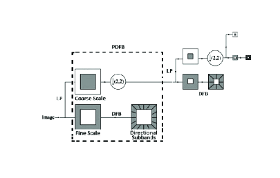
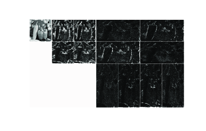
Contourlet transform includes one or many PDFB stages. In the contourlet transform, multiscale and directional decomposition stages are independent of each other and different scales can be decomposed into different numbers of directions. The contourlet transform provides a high level of flexibility in decomposition while being close to critically sampled [18]. Other directional representations are significantly overcomplete or provide a fixed number of directions. The subbands of contourlet transform for the Peppers image have been shown in Fig. 2. It is clear from this figure that only contourlets that fit with both location and direction of the image edges produce significant coefficients.

Figure 2: Contourlet transform on the Peppers image: The contourlet transform with two pyramidal levels is used which followed by four directions in the first level and eight directions in the second level. Large coefficients are shown in white and small coefficients are shown in black [18]

3 STATISTICAL MODELING

It is known that the contourlet coefficients are highly non-Gaussian [16, 28]. The histograms of these coefficients have heavier tails and more sharply peaked modes at zero compared with that of a Gaussian PDF. Here, using Lagrange-multiplier test, we demonstrate that heteroscedasticity exists in the contourlet coefficients, i.e., their conditional variance is non-constant. This property has not been mentioned before and the proposed models for these coefficients suppose them to be identically distributed [16, 28]. To overcome the inefficiency of the previously proposed models in capturing the heteroscedasticity and the dependency of the contourlet coefficients, we propose using 2D-GARCH model. In the following parts, we review 2D-GARCH model and study whether this model provides a flexible and appropriate tool for the coefficients within the framework of multiscale and directional contourlet analysis of the images. It should be mentioned that in this paper, we use 9-7 biorthogonal filters for multiscale decomposition, and PKVA ladder filters [38] for multi directional decomposition [18].

3.1 2D-GARCH Model

Generalized autoregressive conditional heteroscedasticity (GARCH) model has been proposed by Bollerslev in [29]. GARCH processes are a class of zero mean, serially uncorrelated, but not serially independent processes with non-constant variances conditioned on the past [29]. 2D-GARCH processes are the extension of GARCH in two dimensions [39]. Suppose $f_{ij}$ represents a two dimensional stochastic process that follows 2D-GARCH($p_{1},p_{2}$ ,$q_{1},q_{2}$), where ($p_{1},p_{2}$ ,$q_{1},q_{2}$) denotes the order of the model. We have

$$f_{ij} = \sqrt{h_{ij}}\varepsilon_{ij}$$ (1)

$$h_{ij} = \alpha_{0}+\sum_{k\ell\in\Omega_{1}}{\alpha_{k\ell}f_{i-k,j-\ell}^{2}}+\sum_{k\ell\in\Omega_{2}}{\beta_{k\ell}h_{i-k,j-\ell}},$$ (2)

where $\varepsilon_{ij}$ represents an i.i.d two-dimensional stochastic process with standard normal distribution ($\varepsilon_{ij}$$\sim$$\mathcal{N}(0,1)$) and

$$\Omega_{1} = \{k\ell\left|{0\leq k\leq q_{1},0\leq\ell\leq q_{2}}\right.,(k\ell)\neq(0,0)\}$$

$$\Omega_{2} = \{k\ell\left|{0\leq k\leq p_{1},0\leq\ell\leq p_{2}}\right.,(k\ell)\neq(0,0)\}.$$

The conditional variance of $f_{ij}$ is $h_{ij}$ and the conditional distribution of $f_{ij}$ can be formulated as:

$$p(f_{ij}\left|{\psi_{ij}}\right.)=\frac{1}{{\sqrt{2\pi h_{ij}}}}\exp(\frac{{-f_{ij}^{2}}}{{2h_{ij}}}),$$ (3)

where $\psi_{ij}$ is the information set defined as

$$\psi_{ij}=\{\{f_{i-k,j-\ell}\}_{k,\ell\in\Omega_{1}},\{h_{i-k,j-\ell}\}_{k,\ell\in\Omega_{2}}\}.$$

The model parameters are $\Gamma$ = $\{\{\alpha_{0}$, $\alpha_{01}$ , $\cdots,\alpha_{q_{1}q_{2}},\beta_{01},\cdots,\beta_{p_{1}p_{2}}\}\}$ that should be estimated. We use maximum likelihood estimation and the likelihood function can be formulated as

$$LF(\Gamma)=\prod\limits_{ij\in\Phi}{p(f_{ij}\left|{\psi_{ij})}\right.},$$ (4)

where $\Phi=\{ij|{1\leq i\leq M,1\leq j\leq N\}}$ is the sample space of size $M\times N$.

Table 1: Results of Engle and two dimensional [41] hypothesis tests for the presence of 2D-GARCH effect in the eight contourlet subbands of the finest scale for the Peppers image.

	scan	H	pValue	GARCHstat
	vertical	1	0	941.8335
subband	horizontal	1	0	3.9431e+003
1	diagonal	1	0	5.1349e+003
	two dimensional	1	0	1.0166e+004
	vertical	1	0	2.6268e+004
subband	horizontal	1	0	2.3267e+003
2	diagonal	1	0	633.5300
	two dimensional	1	0	2.1819e+004
	vertical	1	0	7.7814e+003
subband	horizontal	1	0	2.4306e+003
3	diagonal	1	0	3.3464e+003
	two dimensional	1	0	7.1432e+003
	vertical	1	0	553.8294
subband	horizontal	1	0	1.7055e+003
4	diagonal	1	0	1.3882e+003
	two dimensional	1	0	6.8305e+003
	vertical	1	0	1.5818e+003
subband	horizontal	1	0	71.1390
5	diagonal	1	0	2.9839e+003
	two dimensional	1	0	1.2155e+004
	vertical	1	0	3.1624e+003
subband	horizontal	1	0	1.1515e+004
6	diagonal	1	0	2.8019e+003
	two dimensional	1	0	6.9759e+003
	vertical	1	0	6.2005e+003
subband	horizontal	1	0	2.6225e+004
7	diagonal	1	0	1.7621e+003
	two dimensional	1	0	2.5357e+004
	vertical	1	0	2.5334e+003
subband	horizontal	1	0	1.4457e+003
8	diagonal	1	0	5.9819e+003
	two dimensional	1	0	8.1015e+003

3.2 2D-GARCH Modeling of the Contourlet Coefficients

Here, we study the compatibility of 2D-GARCH model with the contourlet coefficients. In this way, we carried out extensive simulations on a large number of images. But, due to the space limitation, we present some limited results. 2D-GARCH is a heteroscedastic model that allows the conditional variance to change over two dimensions with a special structure of the dependencies as described in section 3.1. To check the suitability of the 2D-GARCH model for the contourlet coefficients, we should examine the heteroscedasticity of these coefficients and their compatibility with the special type of dependency provided by 2D-GARCH model. In this way, two LM tests have been proposed before [40, 41] and we use them:
1) LM test proposed by Engle in [40]: This test checks the null hypothesis that no GARCH effects exist. It can be used for one dimensional signals. Comparing the structure of conditional variance in 1D-GARCH and 2D-GARCH models, we can conclude that to test the two dimensional GARCH effect, we can apply it for horizontal, vertical, and diagonal scans of the contourlet subbands.
2) LM test proposed in [41, 42] that examines the two-dimensional GARCH effect.
The results of applying these two hypothesis tests for the eight directional subbands in the finest scale of the Peppers image have been shown in table 1. For other test images, similar results have been obtained. In this table “H” is a Boolean decision variable that “1” indicates acceptance of the alternative hypothesis that GARCH effects exist, “pValue” is the significance level at which this test rejects the null hypothesis, and “GARCHstat” indicates GARCH test statistic. The significance level is $0.05$ . This table demonstrates the existence of two dimensional heteroscedasticity in the contourlet coefficients that can be efficiently captured using 2D-GARCH model.
To study the statistical significance of the reported results, we perform the LM tests on the eight directional subbands in the finest scale of 50 natural images. Table 2 reports the mean and standard deviation of the results. All of the computed GARCH test statistics “GARCHstat”s are large. Since the standard deviation of “GARCHstat” is also large, we report the minimum and maximum value of “GARCHstat”, too. It is obvious from this table that all of the tested subbands are heteroscedastic. So, we should mention this property in modelling the contourlet subbands .

• Table 2: Results of Engle and two dimensional [41] hypothesis tests for the presence of 2D-GARCH effect in the contourlet subbands of 50 natural images.

  scan	H		pValue		GARCHstat
  	mean	std	mean	std	mean	std	min	max
  vertical	1	0	0	0	4.83e+003	2.04e+003	589.23	1.00e+004
  horizontal	1	0	0	0	4.87e+003	2.23e+003	571.51	1.22e+004
  diagonal	1	0	0	0	5.58e+003	2.28e+003	2.43e+003	1.42e+004
  two dimensional	1	0	0	0	1.11e+004	2.07e+003	7.29e+003	1.74e+004

Figure 3: Histograms of the contourlet coefficients for Peppers image: (a) directional subband in the first pyramidal level (b) directional subband in the third pyramidal level

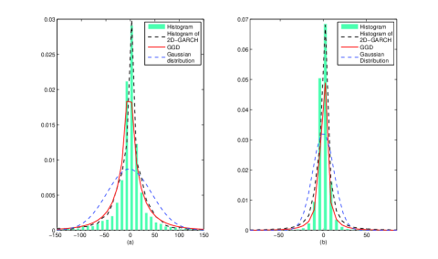
Also, we check the compatibility between the histograms of contourlet coefficients and the 2D-GARCH model. Fig. 3 presents the histograms of two contourlet subbands of Peppers image and the histograms of the best fitted 2D-GARCH model. This figure also shows the best fitted Gaussian and Generalized Gaussian (GG) distributions. It is clear from this figure that 2D-GARCH model provides a better fit to the data. We have obtained similar results for other test images.

4 WATERMARK EMBEDDING

To embed the watermark, we use an additive spread spectrum scheme in the contourlet domain. First, we apply the contourlet transform to the original image. To increase the robustness of the watermark, we insert the watermark in the most significant direction of the image. In this way, we compute the energy of each directional subband in the finest scale and select the subband with the highest energy to embed the watermark. Let ${\bf{f}}=\{f_{ij}|i=1,...,M,j=1,...,N\}$ denotes the selected subband of the original image. We use bold type to denote two dimensional vectors. The rule for additive embedding of the watermark sequence in this subband is

$$g_{ij}=f_{ij}+\gamma s_{ij}=f_{ij}+w_{ij},$$ (5)

where ${\bf{s}}=\{s_{ij}|i=1,...,M,j=1,...,N\}$ denotes the watermark sequence used for marking the contourlet subband, ${\bf{g}}=\{g_{ij}|i=1,...,M,j=1,...,N\}$ denotes the watermarked contourlet subband, and $\gamma$ is the embedding power. ${\bf{s}}$ is a bipolar watermark taking the values $-1$ and $1$ with the same probability. It is obtained by using a pseudorandom sequence (PRS) generator with an initial state depends on the value of a secret key. The final watermark signal $w_{ij}=\gamma s_{ij}$ is generated by the multiplication of the pseudorandom sequence $s_{ij}$ and the embedding power $\gamma$ [10]. $\gamma$ controls the watermark to document ratio (WDR).

5 WATRMARK DETECTION BASED ON 2D-GARCH MODEL

For copyright protection, the detector needs to verify the existence of a known watermark in a given image [10, 16]. Using (5), the additive watermark detection for copyright protection in the contourlet domain can be mathematically formulated as the binary hypothesis test:

$$\mathcal{H}_{0} : g_{ij}=f_{ij}$$ (6)

$$\mathcal{H}_{1} : g_{ij}=f_{ij}+w_{ij}$$ (7)

in which, we verify the existence of $w_{ij}$ in the contourlet coefficients of an image. Here, $\mathcal{H}_{0}$ and $\mathcal{H}_{1}$ denote the null and alternative hypotheses, respectively. In this work, we use a Bayesian log-likelihood ratio test (LLRT) to detect the watermark. It should be mentioned that a detector based on LLRT maximizes the probability of detection (deciding $\mathcal{H}_{1}$ when $\mathcal{H}_{1}$ is true) for a fixed probability of false-alarm (deciding $\mathcal{H}_{1}$ when $\mathcal{H}_{0}$ is true). The Bayesian LLRT is given by

$$\log\{\Lambda({\bf{g}})\}=\log\{\frac{p({\bf{g}}|\mathcal{H}_{1})}{p({\bf{g}}|\mathcal{H}_{0})}\}{\begin{array}[]{c}1\\[-2.84544pt] >\\[-5.69046pt] <\\[-2.84544pt] 0\end{array}}log\{k\frac{P(\mathcal{H}_{0})}{P(\mathcal{H}_{1})}\}=T$$ (8)

where $p({\bf{g}}|\mathcal{H}_{0})$ and $p({\bf{g}}|\mathcal{H}_{1})$ are the pdfs of ${\bf{g}}$ under the conditions $\mathcal{H}_{0}$ and $\mathcal{H}_{1}$, respectively, $k$ is a constant denotes the ratio of false alarm cost to the miss-detection (deciding $\mathcal{H}_{0}$ when $\mathcal{H}_{1}$ is true) cost. $P(\mathcal{H}_{0})$ and $P(\mathcal{H}_{1})$ are the probabilities of null and alternative hypotheses, respectively. To minimize the probability of miss-detection for a bounded false alarm probability, the threshold $T$ is computed using Neyman–Pearson criteria.
To design an efficient detector using (8), the correct choice of priors for the contourlet coefficients is certainly a very important factor. As studied in section 3.2, there is a good compatibility between 2D-GARCH model and the contourlet coefficients. So, we design a watermark detector based on this model. Assume that the contourlet coefficients of the original image ${\bf{f}}$ follow 2D-GARCH model. Using (3), (6), and (7), the log-likelihood ratio given in (8) can be written as:

$$\log\{\Lambda({\bf{g}})\} = \log\frac{\prod\limits_{ij\in\Phi}{p(g_{ij}-w_{ij}\left|{\psi_{ij})}\right.}}{\prod\limits_{ij\in\Phi}{p(g_{ij}\left|{\psi_{ij})}\right.}}$$ (9)

$$= \log\frac{\prod\limits_{ij\in\Phi}{\frac{1}{{\sqrt{2\pi h_{ij}}}}\exp(\frac{{-(g_{ij}-w_{ij})^{2}}}{{2h_{ij}}})}}{\prod\limits_{ij\in\Phi}{\frac{1}{{\sqrt{2\pi h_{ij}}}}\exp(\frac{{-g_{ij}^{2}}}{{2h_{ij}}})}}$$ (10)

where $\psi_{ij}$ and $\Phi$ are as defined in section 3.1. Substituting $h_{ij}$ from (2) in (10), the log-likelihood ratio can be formulated as (11).

• $$\log \{\Lambda({\bf{g}})\}=\log\frac{\prod\limits_{ij\in\Phi}{\frac{1}{{\sqrt{2\pi\alpha_{0}+\sum_{k\ell\in\Omega_{1}}{\alpha_{k\ell}(g_{i-k,j-\ell}-w_{i-k,j-\ell})^{2}}+\sum_{k\ell\in\Omega_{2}}{\beta_{k\ell}h_{i-k,j-\ell}}}}}\exp(\frac{{-(g_{ij}-w_{ij})^{2}}}{{2\alpha_{0}+\sum_{k\ell\in\Omega_{1}}{\alpha_{k\ell}(g_{i-k,j-\ell}-w_{i-k,j-\ell})^{2}}+\sum_{k\ell\in\Omega_{2}}{\beta_{k\ell}h_{i-k,j-\ell}}}})}}{\prod\limits_{ij\in\Phi}{\frac{1}{{\sqrt{2\pi\alpha_{0}+\sum_{k\ell\in\Omega_{1}}{\alpha_{k\ell}g_{i-k,j-\ell}^{2}}+\sum_{k\ell\in\Omega_{2}}{\beta_{k\ell}h_{i-k,j-\ell}}}}}\exp(\frac{{-g_{ij}^{2}}}{{2\alpha_{0}+\sum_{k\ell\in\Omega_{1}}{\alpha_{k\ell}g_{i-k,j-\ell}^{2}}+\sum_{k\ell\in\Omega_{2}}{\beta_{k\ell}h_{i-k,j-\ell}}}})}}$$ (11)

  $$= \sum\limits_{ij\in\Phi}-\log\sqrt{{\sum_{k\ell\in\Omega_{1}}{\alpha_{k\ell}(g_{i-k,j-\ell}-w_{i-k,j-\ell})^{2}}+\sum_{k\ell\in\Omega_{2}}{\beta_{k\ell}h_{i-k,j-\ell}}}}+\log\sqrt{{\sum_{k\ell\in\Omega_{1}}{\alpha_{k\ell}g_{i-k,j-\ell}^{2}}+\sum_{k\ell\in\Omega_{2}}{\beta_{k\ell}h_{i-k,j-\ell}}}}$$

  $$+ \sum\limits_{ij\in\Phi}\left[\frac{{g_{ij}^{2}}}{{2\alpha_{0}+\sum_{k\ell\in\Omega_{1}}{\alpha_{k\ell}g_{i-k,j-\ell}^{2}}+\sum_{k\ell\in\Omega_{2}}{\beta_{k\ell}h_{i-k,j-\ell}}}}+\frac{{-(g_{ij}-w_{ij})^{2}}}{{2\alpha_{0}+\sum_{k\ell\in\Omega_{1}}{\alpha_{k\ell}(g_{i-k,j-\ell}-w_{i-k,j-\ell})^{2}}+\sum_{k\ell\in\Omega_{2}}{\beta_{k\ell}h_{i-k,j-\ell}}}}\right]$$

  $$= \sum\limits_{ij\in\Phi}\log\sqrt{\frac{\sum_{k\ell\in\Omega_{1}}{\alpha_{k\ell}g_{i-k,j-\ell}^{2}}+\sum_{k\ell\in\Omega_{2}}{\beta_{k\ell}h_{i-k,j-\ell}}}{\sum_{k\ell\in\Omega_{1}}{\alpha_{k\ell}(g_{i-k,j-\ell}-w_{i-k,j-\ell})^{2}}+\sum_{k\ell\in\Omega_{2}}{\beta_{k\ell}h_{i-k,j-\ell}}}}+\sum\limits_{ij\in\Phi}[\frac{{g_{ij}^{2}}}{{2\alpha_{0}+\sum_{k\ell\in\Omega_{1}}{\alpha_{k\ell}g_{i-k,j-\ell}^{2}}+\sum_{k\ell\in\Omega_{2}}{\beta_{k\ell}h_{i-k,j-\ell}}}}$$

  $$+ \frac{{-(g_{ij}-w_{ij})^{2}}}{{2\alpha_{0}+\sum_{k\ell\in\Omega_{1}}{\alpha_{k\ell}(g_{i-k,j-\ell}-w_{i-k,j-\ell})^{2}}+\sum_{k\ell\in\Omega_{2}}{\beta_{k\ell}h_{i-k,j-\ell}}}}]$$

Figure 4: Histograms of log-likelihood ratio $\log\Lambda$ under (a) $\mathcal{H}_{0}$ and (b) $\mathcal{H}_{1}$ conditions. Vertical bars show the normalized histogram , Gaussian distribution depicted in red dashed line. (Peppers image, directional subband in the finest scale with the highest energy)

5.1 Analysis of the Detector Performance

To analyze the performance of our proposed detector in terms of its probability of false alarm $P_{F}$ and its probability of detection $P_{D}$, first, we should investigate the distribution of log-likelihood ratio $\log\Lambda$ in (11). In the following, by using normalized histograms, Kolmogrov-Smirnov test and the estimated kurtosis, we demonstrate that $\log\Lambda$ could be well approximated by a Gaussian distribution.
We obtain the histogram of log-likelihood ratio under the conditions $\mathcal{H}_{0}$ and $\mathcal{H}_{1}$ by repeating the embedding step 1000 times. Each time starts with a uniquely-defined key to randomly generate the watermark sequence. In the rest of this paper, we use a similar way to obtain the experimental results. 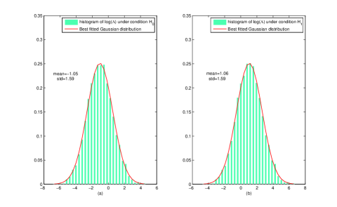We focus on the contourlet subband in which the watermark is embedded, i.e, the directional subband in the finest scale with the highest energy. The histograms of log-likelihood ratio for the most energetic subband in the finest scale of the Peppers image under the conditions $\mathcal{H}_{0}$ and $\mathcal{H}_{1}$ have been shown in Fig. 4.a and Fig. 4.b, respectively (WDR= -50 dB). This figure also represents the best fitted Gaussian distribution. We can see that the Gaussian distribution has been well fitted to the histograms. Also, it is clear from Fig. 4 that the mean of $\log\Lambda$ under the conditions $\mathcal{H}_{0}$ and $\mathcal{H}_{1}$ have approximately the same amplitude and opposite sign, and the variances under these conditions are approximately equal. It should be mentioned that the modeling results of different images are similar.

Table 3: Results of the KS test for $\log\Lambda$ of Peppers image (directional subband in the finest scale with the highest energy) under the conditions $\mathcal{H}_{0}$ and $\mathcal{H}_{1}$.

WDR (dB)		-50	-52	-54	-56	-58	-60
	$H$	0	0	0	0	0	0
$\mathcal{H}_{0}$	$KSD$	0.0178	0.0166	0.0176	0.0169	0.0157	0.0150
	$H$	0	0	0	0	0	0
$\mathcal{H}_{1}$	$KSD$	0.0168	0.0172	0.0167	0.0168	0.0151	0.0152

Now, we use the Kolmogrov-Smirnov (KS) test to quantify the results. This test evaluates the compatibility between the distribution of a sample data $p(x)$ and a given PDF $p_{1}(x)$. KS method is a binary hypothesis test. The null hypothesis ($H_{0}$) denotes that the distribution $p(x)$ is same as $p_{1}(x)$. To employ this test, first, the KS distance ($KSD$) should be computed:

$$KSD=\max_{-\infty<x<\infty}|P(x)-P_{1}(x)|.$$ (12)

where $P(x)$ and $P_{1}(x)$ denote the corresponding cumulative distribution functions. Then, KS distance is compared with a threshold to decide between two hypotheses ($H_{0}$ and $H_{1}$). This threshold is determined based on the significance level of the test. We perform KS test to examine the compatibility between the density of $\log\Lambda$ ($p(x)$) with the Gaussian distribution ($p_{1}(x)$). Table 3 reports the accepted hypothesis “$H$” and $KSD$ in different WDRs for the Peppers image. “$H$” takes the values “0” and “1” to indicate $H_{0}$ and $H_{1}$, respectively. These results verify that $\log\Lambda$ can be well approximated with the Gaussian distribution.
Also, the sample kurtosis of $\log\Lambda$ (fourth moment divided by the square of the second moment) in different WDRs have been reported in table 4. All of the estimated kurtoses are close to the value of three, which is expected for a Gaussian distribution.
Finally, to demonstrate the statistical significance of the reported results, we perform the KS test on $\log\Lambda$ of contourlet coefficients for 50 natural images (the subbands in the finest scale with the highest energy) and also compute the corresponding kurtoses. The mean and standard deviation of the results have been reported in table 5 and table 6. It is evident from these tables that for all of the tested subbands, $\log\Lambda$ can be efficiently approximated by the Gaussian distribution.

Table 4: kurtosis for $\log\Lambda$ of Peppers image (directional subband in the finest scale with the highest energy) under the conditions $\mathcal{H}_{0}$ and $\mathcal{H}_{1}$.

WDR (dB)	-50	-52	-54	-56	-58	-60
$\mathcal{H}_{0}$	2.9346	3.0898	2.9808	2.9213	2.9451	2.8006
$\mathcal{H}_{1}$	2.9370	3.0902	2.9810	2.9197	2.9450	2.8012

Table 5: mean and standard deviation of the KS test results for $\log\Lambda$ of 50 natural images (directional subband in the finest scale with the highest energy) under the conditions $\mathcal{H}_{0}$ and $\mathcal{H}_{1}$.

mean
WDR (dB)		-50	-52	-54	-56	-58	-60
	$H$	0	0	0	0	0	0
$\mathcal{H}_{0}$	$KSD$	0.0203	0.0212	0.0196	0.0201	0.0199	0.0214
	$H$	0	0	0	0	0	0
$\mathcal{H}_{1}$	$KSD$	0.0202	0.0207	0.0197	0.0202	0.0198	0.0212
std
WDR (dB)		-50	-52	-54	-56	-58	-60
	$H$	0	0	0	0	0	0
$\mathcal{H}_{0}$	$KSD$	0.0060	0.0056	0.0048	0.0051	0.0050	0.0062
	$H$	0	0	0	0	0	0
$\mathcal{H}_{1}$	$KSD$	0.0053	0.0051	0.0051	0.0056	0.0051	0.0058

Table 6: mean and standard deviation of kurtosis for $\log\Lambda$ of 50 natural image (directional subband in the finest scale with the highest energy) under the conditions $\mathcal{H}_{0}$ and $\mathcal{H}_{1}$.

mean
WDR (dB)	-50	-52	-54	-56	-58	-60
$\mathcal{H}_{0}$	2.9146	2.8911	2.9485	2.9305	2.9326	2.9474
$\mathcal{H}_{1}$	2.9181	2.8900	2.9506	2.9357	2.9325	2.9608
std
WDR (dB)	-50	-52	-54	-56	-58	-60
$\mathcal{H}_{0}$	0.2301	0.1672	0.1614	0.2143	0.2126	0.1710
$\mathcal{H}_{1}$	0.2248	0.1664	0.1722	0.2229	0.2129	0.1674

So, we assume that $\log\Lambda$ follows the Gaussian distribution. Based on this assumption, the probability of false alarm and the probability of detection can be computed as [10]:

$$P_{F}=Q\left(\frac{T-\mu_{0}}{\sigma_{0}}\right)\quad P_{D}=Q\left(\frac{T-\mu_{1}}{\sigma_{1}}\right)$$ (13)

where $Q(x)$ is defined as $Q(x)=\frac{1}{\sqrt{2\pi}}\int_{x}^{\infty}\exp(-\frac{u^{2}}{2})du$ and $T$ is the threshold in (8). $\mu_{0},\sigma_{0},\mu_{1},\sigma_{1}$ are the mean and standard deviation of $\log\Lambda$ conditioned on the two hypotheses, $\mathcal{H}_{0}$ and $\mathcal{H}_{1}$. From (13), we have

$$T=\sigma_{0}Q^{-1}(P_{F})+\mu_{0}$$ (14)

Using (13) and (14), the receiver operating characteristic (ROC) of the watermark detector that presents the function relation between the probabilities of detection ($P_{D}$) and false alarm ($P_{F}$ ) can be formulated as

$$P_{D}=Q\left(\frac{1}{\sigma_{1}}\left[\sigma_{0}Q^{-1}(P_{F})+\mu_{0}-\mu_{1}\right]\right).$$ (15)

Therefore, to analyze the performance of the proposed detector, $\mu_{0},\sigma_{0},\mu_{1},$ and $\sigma_{1}$ should be estimated. In Appendix A, we compute them.
We should notice that the watermark signal is very small in comparison with the original contourlet coefficients. Therefore, similar to some previously proposed watermark detectors such as [10, 11], we suppose that the insertion of the watermark doesn’t change the parameters of the statistical model significantly. We estimate the parameters of 2D-GARCH model using the received image, so, the proposed watermark detector is blind.
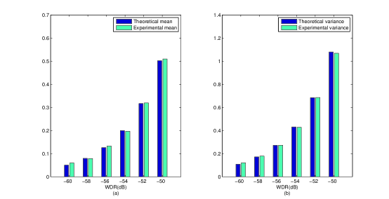
Here, we examine the validity of the theoretical mean and variance of $\log\Lambda$ under $\mathcal{H}_{0}$ and $\mathcal{H}_{1}$ computed in (17)-(22) by using the mean and variance of the experimental results of the test statistic. Since we have $\mu_{0}=-\mu_{1},\quad\sigma_{0}^{2}=\sigma_{1}^{2}$, reporting the results under one of the hypotheses is sufficient. We performed Monte Carlo experiments using the 2D-GARCH detector and compute the mean and the variance of the experimental results. The experimental and the theoretical means and variances as a function of WDR have been plotted in Fig. 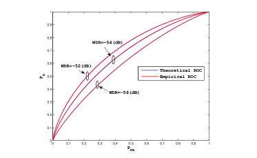5.a and fig. 5.b. Also, Fig. 6 shows the experimental and the theoretical ROCs for three different WDRs. It is clear from Fig. 5 and Fig. 6 that the empirical measurements fit the theoretical estimates.

Figure 5: (a) Empirical and theoretical means of test statistic, (b) Empirical and theoretical variances of test statistic. (Peppers image, directional subband in the finest scale with the highest energy)

Figure 6: Empirical and theoretical ROCs (Peppers image, directional subband in the finest scale with the highest energy)

6 EXPERIMENTAL RESULTS

In this section, we study the performance of the proposed watermark detector experimentally. For multiscale decomposition, 9-7 biorthogonal filters with two levels of pyramidal decomposition are used. In the multi directional decomposition stage, PKVA ladder filters are employed. The finest scale is decomposed into eight directional subbands and the subband with the highest energy is selected to embed the watermark. We use 2D-GARCH(1,1,1,1). To evaluate the efficiency of the proposed watermark detector, we performed simulations on a large number of images. However, due to the space limitations, we report the results of four $512\times 512$ grayscale representative images, namely, Peppers, Living room, Lake, and Pirate. Also, we used 50 natural images and report the averaged results. In the following, first, we assess the performance of the contourlet domain 2D-GARCH detector without any kind of attack. Then, since copyright protection needs robust watermark detector, we study the robustness of the proposed detector under different kinds of attacks. Also, we compare the proposed method with the other related detectors.

6.1 Performance without attack

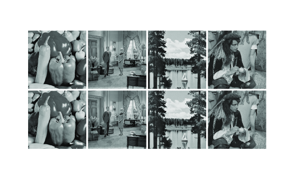
In fig. 7, four test images and the watermarked version of them with $WDR=-50dB$ are represented. This figure confirms that the proposed method satisfies the watermark invisibility.
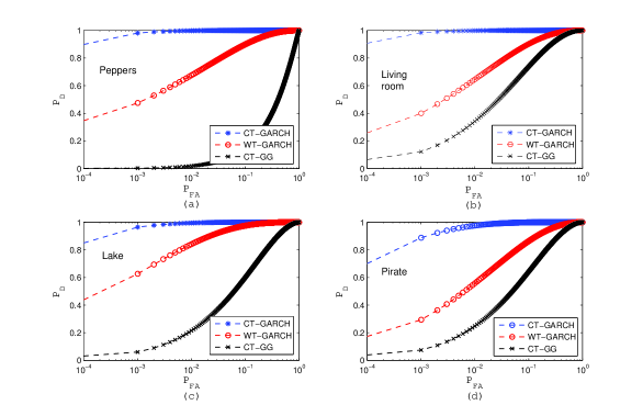
Now, we use ROC to study the performance of the proposed detector and to compare it with the other related detectors. Fig. 8 presents the ROCs of the contourlet domain 2D-GARCH based detector (CT-GARCH) for the four test images. This figure also compares the ROCs of the proposed method with two other detectors: 1) contourlet domain generalized Gaussian based detector (CT-GG). It should be mentioned that using generalized Gaussian distribution for the contourlet coefficients has been proposed in some papers such as [28]. 2) wavelet domain 2D-GARCH based detector (WT-GARCH). For the wavelet domain 2D-GARCH based detector, 2D-GARCH(1,1,1,1) is used and the watermark is embedded in the detail subbands of the second level decomposition. We use “Daubechies” wavelet with four vanishing moments. This figure shows that the proposed detector provides the highest probability of detection for any chosen value of the false alarm.

Figure 7: Test images: “Peppers”, “Living Room”,‘Lake‘”, and “Pirate”, up to down: Original images, and watermarked images using the proposed scheme with WDR=-50 dB

Figure 8: ROC of the three statistical detectors. Test images are (a) Peppers, (b) Living Room, (c) Lake, and (d) Pirate. (WDR=-50 dB)

6.2 Performance under attacks

In this section, we assess the performance of the contourlet domain 2D-GARCH based detector under some standard attacks, i.e., JPEG compression, median and Gaussian filtering, scaling, and a combinational attack. Also, we compare the performance of the CT-GARCH detector with the CT-GG and WT-GARCH detectors. To study the detection performance quantitatively, the area under the ROC curve (AUROC) has been used [11, 44].
Table 7 reports the AUROC results of the CT-GARCH, CT-GG, and WT-GARCH detectors under JPEG compression attack for WDR = -45 dB and WDR = -50 dB. It is clear from this table that the CT-GARCH detector outperforms the other detectors.

Table 7: auroc results under JPEG compression (QF=60) attack

WDR = -50 dB
Image	CT-GG	WT-GARCH	CT-GARCH
	Detector	Detector	Detector
Peppers	0.7887	0.8512	0.9814
Living room	0.7527	0.9294	0.7527
Lake	0.8968	0.0.8393	0.9488
Pirate	0.6818	0.8166	0.9145
WDR = -45 dB
Peppers	0.8634	0.9407	1.0000
Living room	0.9718	0.9765	1.0000
Lake	0.9916	0.9338	0.9964
Pirate	0.8449	0.9143	0.9948

The AUROC results of the CT-GARCH, CT-GG, and WT-GARCH detectors under scaling attack have been reported in table 8 (WDR = -45 dB and WDR = -50 dB). We can see the higher performance of CT-GARCH detector under scaling attack.
The median filter is a nonlinear filter which produces a smoother image. This filter might cause to fail in watermark detection and a detector performance under this attack is demanding. Table 9 and table 10 represent the AUROC results of the detectors in WDR = -45 dB and WDR = -50 dB under median and Gaussian filtering attacks, respectively (with the windows of size $5\times 5$). For Gaussian filtering, the standard deviation of the filter is set to $w/6$ where $w$ is the size of window. Due to the very high efficiency of the proposed method under Gaussian filtering attack in WDR = -45 dB and WDR = -50 dB, we also report the results under this attack for very weak watermark signal WDR = -60 dB. The reported results demonstrate the efficiency of the CT-GARCH detector.
To investigate the performance of the detectors under combinational attacks, table 11 reports the AUROC results under combination of the Gaussian filtering (window size = $5\times 5$) and additive white Gaussian noise (AWGN) attacks (std=10). The high performance of the proposed method under this combinational attack is obvious from this table.
Finally, to investigate the statistical significance of the reported results, we perform the robustness tests on 50 natural images. The averaged AUROC results over 50 images are reported in table 12 . This table confirms the higher performance of the proposed method (CT-GARCH) in comparison with CT-GG and WT-GARCH.

Table 8: AUROC results under scaling attack (scaling factor = 0.75)

WDR = -50 dB
Image	CT-GG	WT-GARCH	CT-GARCH
	Detector	Detector	Detector
Peppers	0.7877	0.7516	0.9920
Living room	0.7578	0.8335	0.9986
Lake	0.7510	0.8532	0.9941
Pirate	0.8174	0.7870	0.9834
WDR = -45 dB
Peppers	0.8431	0.9026	1.0000
Living room	0.8748	0.9115	1.0000
Lake	0.8334	0.9319	1.0000
Pirate	0.8873	0.9128	1.0000

Table 9: AUROC results under median filtering attack (window size = $5\times 5$)

WDR = -50 dB
Peppers	0.8237	0.8037	0.9971
Living room	0.9994	0.8820	1.0000
Lake	0.9959	0.7193	0.9996
Pirate	0.6258	0.9964	0.8784
WDR = -45 dB
Peppers	1.0000	0.8965	1.0000
Living room	1.0000	0.9676	1.0000
Lake	1.0000	0.9140	1.0000
Pirate	1.0000	0.9742	1.0000

Table 10: AUROC results under Gaussian filtering attack (window size = $5\times 5$)

WDR = -60 dB
Image	CT-GG	WT-GARCH	CT-GARCH
	Detector	Detector	Detector
Peppers	0.7000	0.6469	0.9150
Living room	0.5182	0.6264	0.9541
Lake	0.7962	0.6249	0.8556
Pirate	0.8108	0.6622	0.8904
WDR = -50 dB
Peppers	0.9439	0.8565	1.0000
Living room	0.9269	0.8808	1.0000
Lake	0.9152	0.8902	1.0000
Pirate	0.9965	0.8795	1.0000
WDR = -45 dB
Peppers	0.7300	0.9700	1.0000
Living room	0.9993	0.9789	1.0000
Lake	0.9994	0.9362	1.0000
Pirate	1.0000	0.9816	1.0000

Table 11: AUROC results under combination of Gaussian Filtering and AWGN attacks

WDR = -50 dB
Image	CT-GG	WT-GARCH	CT-GARCH
	Detector	Detector	Detector
Peppers	0.8864	0.7773	0.9649
Living room	0.8299	0.7268	0.9936
Lake	0.8732	0.8195	0.9761
Pirate	0.6160	0.7090	0.9772
WDR = -45 dB
Peppers	0.7604	0.8960	1.0000
Living room	0.9556	0.9084	1.0000
Lake	0.5300	0.9143	1.0000
Pirate	0.8686	0.8887	1.0000

Table 12: Average AUROC results for 50 natural images under different types of attacks (WDR = -50 $dB$)

Attack	CT-GG	WT-GARCH	CT-GARCH
type	Detector	Detector	Detector
Compression	0.8463	0.8454	0.9320
(QF=60)
Scaling	0.7863	0.7982	0.9654
(SF=0.75)
Median Filtering	0.9324	0.8864	0.9828
$5\times 5$
Gaussian Filtering	0.9288	0.8705	0.9951
$5\times 5$
Gaussian Filtering	0.7536	0.7585	0.9708
+ AWGN

7 conclusion

This paper proposed a novel watermark detector for contourlet domain additive image watermarking. Watermark detection can be formulated as a binary hypothesis test. Based on Neyman-Pearson criterion, the optimal detector can be achieved using LRT. Selecting the statistical model employed in the LRT is a major issue.
In this paper [2], we have first studied the statistical characteristics of the contourlet coefficients. The heteroscedasticity of these coefficients has been shown using two Lagrange multiplier tests. The previously proposed statistical models usually assume the contourlet coefficients to be identically distributed and cannot capture the heteroscedasticity of these coefficients. So, these models don’t provide a good compatibility with the contourlet coefficients and the watermark detectors based on such models show inadequate performance. To overcome this problem, we studied the compatibility between the contourlet coefficients and 2D-GARCH which is an efficient and flexible heteroscedastic model. Consequently, we designed a watermark detector based on 2D-GARCH model. Our method is based on solid statistical theory and the ROC of 2D-GARCH based detector has been derived analytically. We have studied the experimental efficiency of the proposed detector in detail by conducting several experiments. The robustness of the proposed detector against different kinds of attacks has been evaluated and the superiority of the proposed method compared with some other methods has been shown [1, 2].
This paper is the first work that studies and captures the heteroscedasticity of the contourlet coefficients, and taking into account the heteroscedasticity of the contourlet coefficients can lead to good results in other fields such as contourlet domain image restoration.

Appendix A Appendix A

Here we compute $\mu_{0},\sigma_{0},\mu_{1},$ and $\sigma_{1}$ as defined in section 5.1. To simplify the notation, we define two functions: :

$$\mathcal{X}({\bf F}_{ij},\gamma)=\quad\quad\quad\quad\quad\quad\quad\quad\quad\quad\quad\quad\quad\quad\quad\quad\quad\quad\quad\quad\quad\quad\quad$$

$$\sqrt{\frac{\sum_{k\ell\in\Omega_{1}}{\alpha_{k\ell}f_{i-k,j-\ell}^{2}}+\sum_{k\ell\in\Omega_{2}}{\beta_{k\ell}h_{i-k,j-\ell}}}{\sum_{k\ell\in\Omega_{1}}{\alpha_{k\ell}(f_{i-k,j-\ell}-\gamma)^{2}}+\sum_{k\ell\in\Omega_{2}}{\beta_{k\ell}h_{i-k,j-\ell}}}}\quad\quad\quad\quad$$

$$\mathcal{Y}({\bf F}_{ij},\gamma)=\quad\quad\quad\quad\quad\quad\quad\quad\quad\quad\quad\quad\quad\quad\quad\quad\quad\quad\quad\quad\quad\quad\quad$$

$$0.5(\frac{{{f}_{ij}^{2}}}{{2\alpha_{0}+\sum_{k\ell\in\Omega_{1}}{\alpha_{k\ell}f_{i-k,j-\ell}^{2}}+\sum_{k\ell\in\Omega_{2}}{\beta_{k\ell}h_{i-k,j-\ell}}}})\quad\quad\quad$$

$$+\frac{{-({f}_{ij}-\gamma)^{2}}}{{2\alpha_{0}+\sum_{k\ell\in\Omega_{1}}{\alpha_{k\ell}(f_{i-k,j-\ell}-\gamma)^{2}}+\sum_{k\ell\in\Omega_{2}}{\beta_{k\ell}h_{i-k,j-\ell}}}})\quad$$ (16)

where $\Omega_{1},\Omega_{2},h_{i,j}$ are as defined in section 3.1 and ${\bf F}_{ij}=\{f_{n,m}|1\leq n\leq i,1\leq m\leq j\}$. The watermark sequence is an i.i.d. two dimensional random process which takes the values $+\gamma$ or $+\gamma$ with the same probability. In this case, using (11), the mean of $\log\Lambda$ under the condition $\mathcal{H}_{0}$ can be computed as

$$\mu_{0} = E_{w}(\log\Lambda|\mathcal{H}_{0})=0.5(\sum_{i,j}{\log\mathcal{X}({\bf F}_{ij},\gamma)+\log\mathcal{X}({\bf F}_{ij},-\gamma)})$$ (17)

$$+ 0.5(\sum_{i,j}{\mathcal{Y}({\bf F}_{ij},\gamma)+\mathcal{Y}({\bf F}_{ij},-\gamma)})$$

where $E_{w}(.)$ denotes the expectation on $w$. To calculate the variance of $\log\Lambda$ conditioned on $\mathcal{H}_{0}$, first $E_{w}(\log\Lambda|\mathcal{H}_{0})^{2}$ is computed:

$$E {}_{w}(\log\Lambda|\mathcal{H}_{0})^{2}=E_{w}(\sum_{i,j}\log\mathcal{X}({\bf F}_{ij},w)+\sum_{i,j}\mathcal{Y}({\bf F}_{ij},w))^{2}$$ (18)

$$= 0.5(\sum_{i,j}\log\mathcal{X}({\bf F}_{ij},\gamma)+\sum_{i,j}\mathcal{Y}({\bf F}_{ij},\gamma))^{2}$$

$$+ (\sum_{i,j}\log\mathcal{X}({\bf F}_{ij},-\gamma)+\sum_{i,j}\mathcal{Y}({\bf F}_{ij},-\gamma))^{2}$$

then, we have

$$\sigma_{0}^{2}=E_{w}(\log\Lambda|\mathcal{H}_{0})^{2}-\mu_{0}$$ (19)

In the same way, we can compute the mean of $\log\Lambda$ conditioned on $\mathcal{H}_{1}$ as

$$\mu_{1} = E_{w}(\log\Omega|\mathcal{H}_{1})=0.5(\sum_{i,j}{\log\mathcal{X}^{-1}({\bf F}_{ij},\gamma)+\log\mathcal{X}^{-1}({\bf F}_{ij},-\gamma)})$$ (20)

$$+ 0.5(\sum_{i,j}{-\mathcal{Y}({\bf F}_{ij},\gamma)-\mathcal{Y}({\bf F}_{ij},-\gamma)}).$$

To compute the variance of $\log\Lambda$ conditioned on $\mathcal{H}_{1}$, we have

$$E_{w}(\log\Omega|\mathcal{H}_{1})^{2} = E_{w}(\sum_{i,j}\log\mathcal{X}^{-1}({\bf F}_{ij},w)+\sum_{i,j}-\mathcal{Y}({\bf F}_{ij},w))^{2}$$ (21)

$$= 0.5(\sum_{i,j}\log\mathcal{X}^{-1}({\bf F}_{ij},\gamma)+\sum_{i,j}-\mathcal{Y}({\bf F}_{ij},\gamma))^{2}$$

$$+ (\sum_{i,j}\log\mathcal{X}^{-1}({\bf F}_{ij},-\gamma)+\sum_{i,j}-\mathcal{Y}({\bf F}_{ij},-\gamma))^{2}$$

and

$$\sigma_{1}^{2} = E_{w}(\log\Omega|\mathcal{H}_{1})^{2}-\mu_{1}$$ (22)

References

- [1] I. J. Cox, M. L. Miller, J. A. Bloom, J. Fridrich, and T. Kolker,Digital Watermarking and steganography, Second ed. Morgan Kaufmann Publishers, 2008.
- [2] Q. Cheng and T. S. Huang, “Robust optimum detection of transform domain multiplicative watermarks”, IEEE Trans. Signal Process., vol. 51, no. 4, pp. 906–924, Apr. 2003.
- [3] W. Liu, L. Dong, and W. Zeng, “Optimum detection for spread-spectrum watermarking that employs self-masking,” IEEE Trans. Inf. Forensics Security, vol. 2, no. 4, pp. 645–654, Dec. 2007.
- [4] A. Valizadeh, and Z. J. Wang, “An Improved Multiplicative Spread Spectrum Embedding Scheme for Data Hiding”, IEEE Trans. Inf. Forensics Security, vol. 7, no. 4, pp. 1127–1143, Aug. 2012.
- [5] M. Amirmazlaghani, M. Rezghi, and H. Amindavar, “A novel robust scaling image watermarking scheme based on Gaussian Mixture Model”, Expert Systems with Applications, vol. 42, pp. 1960–1971, 2015.
- [6] B. Chen and G. W. Wornell, “Quantization index modulation: A class of provably good methods for digital watermarking and information embedding, IEEE Trans. Inf. Theory, vol. 47, no. 4, pp. 1423 1443, Apr. 2001.
- [7] O. E. Okman and G. B. Akar, ”Quantization index modulation-based image watermarking using digital holography, J. Opt. Soc. Amer., vol. 24, no. 1, pp. 243 252, 2007.
- [8] I. J. Cox, J. Kilian, F. T. Leighton, and T. Shanon, “Secure spread spectrum watermarking for multimedia,” IEEE Trans. Image Process., vol. 6, no. 12, pp. 1673 1687, Dec. 1997.
- [9] X. Huang and B. Zhang, “Statistically robust detection of multiplicative spread-spectrum watermarks,” IEEE Trans. Inf. Forensics Sec., vol. 2, no. 1, pp. 1 -13, Jan. 2007.
- [10] S. M. Mahbubur Rahman, M. Omair Ahmad, and M. N. S. Swamy, “A New statistical detector for DWT-Based additive image watermarking using the Gauss Hermite expansion”, IEEE Trans. Image Processing, vol. 18, no. 8, pp. 1782–1796, Aug. 2009.
- [11] Y. Bian and S. Liang, “Locally optimal detection of image watermarks in the wavelet domain using Bessel K Form distribution”, IEEE Trans. Image Processing, vol. 22, no. 6, pp. 2372–2384, June. 2013.
- [12] V. R. Doncel, N. Nikolaidis, and I. Pitas, ”An optimal detector structure for the Fourier descriptors domain watermarking of 2D vector graphics, IEEE Trans. Vis. Comput. Graph., vol. 13, no. 5, pp. 851 -863, May 2007.
- [13] V. S. Verma, R. K. Jha, and A. Ojha, “Significant region based robust watermarking scheme in lifting wavelet transform domain”, Expert Systems with Applications, vol. 42, no. 21, pp. 8184-8197, Nov. 2015.
- [14] A. Tareef, and A. Al-Ani “A highly secure oblivious sparse coding-based watermarking system for ownership verification”, Expert Systems with Applications, vol. 42, no. 4, pp. 2224-2233, Mar. 2015.
- [15] P. P. Niu, X. Y.Wang, Y.P. Yang, and M. Y. Lu,“A novel color image watermarking scheme in nonsampled contourlet-domain”, Expert Systems with Applications, vol. 38, no. 3, pp. 2081-2098, Mar. 2011.
- [16] H.R. Sadreazami, M. O. Ahmad, and M. N. S. , Swamy, “A Study of multiplicative watermark detection in the contourlet domain using alpha-stable distributions”, IEEE Trans. Image Processing, vol. 23, no. 10, pp. 4348–4360, Oct. 2014.
- [17] M. Rabizadeh, M. Amirmazlaghani, and M. Ahmadian-Attari, “ A New detector for contourlet domain multiplicative image watermarking using Bessel K form distribution”, Journal of Visual Communication and Image Representation, vol. 40, PP. 324-334, 2016.
- [18] M. N. Do and M. Vetterli, “The contourlet transform: An efficient directional multiresolution image representation,” IEEE Trans. Image Process., vol. 14, no. 12, pp. 2091 2106, Dec. 2005.
- [19] S. Ranjbar, F. Zargari, and M. Ghanbari, “A highly robust two-stage Contourlet-based digital image watermarking method”, Signal Processing:Image Communications, vol. 28, no. 10, pp. 1526 1536, Nov. 2013.
- [20] L. Li, X. Yuan, Z. Lu, J. S. Pan, “ Rotation invariant watermark embedding based on scale-adapted characteristic ”, Information Sciences, vol. 180, no. 15, pp. 2875-2888, Aug. 2010.
- [21] X. Y. Wang, A. L. Wang, H. Y. Yang, Y. Zhang, C. P. Wang, “A new robust digital watermarking based on exponent moments invariants in nonsubsampled contourlet transform domain”, Computers & Electrical Engineering, vol. 40, no. 3, pp. 942-955 Apr. 2014.
- [22] H. Song, S. Yu, X. Yang, L. Song, and C. Wang, “Contourlet-based image adaptive watermarking”, Signal Processing:Image Communications, vol. 23, no. 3, pp. 162-178, Mar. 2008.
- [23] M. Jayalakshmi, S.N. Merchant, U.B. Desai, “Blind watermarking in contourlet domain with improved detection”, Proc. Intelligent Information Hiding and Multimedia Signal Processing (IIH-MSP), Pasadena, CA, USA, Dec. 2006.
- [24] M. S. Hsieh, D. C. Tseng, and Y. H. Huang, “Hiding digital watermarks using multiresolution wavelet transform,” IEEE Trans. Ind. Electron., vol. 48, no. 5, pp. 875 -882, May 2001.
- [25] N. Kaewkamnerd and K. Rao, “Wavelet based image adaptive watermarking scheme,” Electron. Lett., vol. 36, no. 4, pp. 312 -313, 2000.
- [26] T. M. Ng and H. K. Garg, “Maximum-likelihood detection in DWT domain image watermarking using Laplacian modeling,” IEEE Signal Process. Lett., vol. 12, no. 4, pp. 285- 288, Apr. 2005.
- [27] A. Nikolaidis and I. Pitas, “Asymptotically optimal detection for additive watermarking in the DCT and DWT domains,” IEEE Trans. Image Process., vol. 12, no. 5, pp. 563 -571, May 2003.
- [28] H. Qu and Y. Peng, “Contourlet coefficient modeling with generalized Gaussian distribution and application,” in Proc. Int. Conf. Audio, Lang., Image Process. (ICALIP), Jul. 2008.
- [29] T. Bollerslev, “Generalized autoregressive conditional heteroscedasticity,” J. Econometrics, vol. 31, pp. 307- 327, 1986.
- [30] M. Amirmazlaghani, H. Amindavar, and A.R. Moghaddamjoo, “Speckle suppression in SAR images using the 2-D GARCH model”, IEEE Trans. Image Processing, vol. 18, no. 2, pp. 250–259, Feb. 2009.
- [31] M. Amirmazlaghani, “Additive watermark detection in wavelet domain using 2D-GARCH model”, Information Science, 370, pp. 1-17, 2016.
- [32] M. Amirmazlaghani and H. Amindavar, “ Image denoising using two-dimensional GARCH model”, in Systems, Signals and Image Processing, pp. 397–400, 2007.
- [33] M Amirmazlaghani, H Amindavar, “Wavelet domain Bayesian processor for speckle removal in medical ultrasound images” IET image processing, vol. 6, no. 5, pp. 580-588, 2012.
- [34] I. W. Selesnick, R. G. Baraniuk, and N. C. Kingsbury, “The dual-tree complex wavelet transform,” IEEE Signal Process. Mag., vol. 22, no. 6, pp. 123 156, Nov. 2005.
- [35] E. J. Cand s and D. L. Donoho, ”Ridgelets: A key to higher-dimensional intermittency?” Philosoph. Trans. Roy. Soc. London A, vol. 357, no. 1760, pp. 2495 2509, 1999.
- [36] E. J. Cand s and D. L. Donoho, “Curvelets A surprisingly effective non-adaptive representation for objects with edges,’ in Curve and Surface Fitting, C. R. A. Cohen and L. Schumaker, Eds. Nashville, TN, USA: Vanderbilt Univ. Press, 2000.
- [37] D. Minh, and M.Vetterli,“Framing pyramids”, IEEE Transactions on Signal Processing, vol. 51, pp. 2329 2342, Sep. 2003.
- [38] S.-M. Phoong, C. W. Kim, P. P. Vaidyanathan, and R. Ansari, “A new class of two-channel biorthogonal filter banks and wavelet bases,” IEEE Trans. Signal Process., vol. 43, no. 3, pp. 649 665, Mar. 1995.
- [39] M. Amirmazlaghani, H. Amindavar, “ A novel wavelet domain statistical approach for denoising SAR images”, in 16th IEEE International Conference on Image Processing (ICIP), pp. 3861-3864, 2009.
- [40] R.F. Engle, “Autoregressive conditional heteroskedasticity with estimates of the variance of U.K. inflation”, Econometrica 50, pp.987-1008,1982.
- [41] M. Amirmazlaghani, and H. Amindavar, “A novel sparse method for despeckling SAR images”, IEEE Trans. Geosci. Remote Sensing, vol.5̇0, no. 12, pp. 5024–5032, Dec. 2012.
- [42] M. Amirmazlaghani, and H. Amindavar, “ Statistical modeling and denoising Wigner–Ville distribution”, Digital Signal Processing, vol. 23, no. 2, pp. 506-513, 2013.
- [43] A. K. Mairgiotis, N. P. Galatsanos, and Y. Yang, “New additive watermark detectors based on a hierarchical spatially adaptive image model,” IEEE Trans. Inf. Forensics Security, vol. 3, no. 1, pp. 29 -37, Mar. 2008.
- [44] A. K. Mairgiotis, N. P. Galatsanos, and Y. Yang, “New additive watermark detectors based on a hierarchical spatially adaptive image model,” IEEE Trans. Inf. Forensics Security, vol. 3, no. 1, pp. 29 -37, Mar. 2008.