EPJ Web of Conferences \woctitleLattice2017
Progress on Complex Langevin simulations of a finite density matrix model for QCD
Abstract
We study the Stephanov model, which is an RMT model for QCD at finite density, using the Complex Langevin algorithm. Naive implementation of the algorithm shows convergence towards the phase quenched or quenched theory rather than to intended theory with dynamical quarks. A detailed analysis of this issue and a potential resolution of the failure of this algorithm are discussed. We study the effect of gauge cooling on the Dirac eigenvalue distribution and time evolution of the norm for various cooling norms, which were specifically designed to remove the pathologies of the complex Langevin evolution. The cooling is further supplemented with a shifted representation for the random matrices. Unfortunately, none of these modifications generate a substantial improvement on the complex Langevin evolution and the final results still do not agree with the analytical predictions.
1 Introduction
Many interesting physical systems have a complex action which impedes Monte Carlo simulations due to the notorious sign problem. In this category belongs QCD at finite baryon density, Yang-Mills theories in the presence of a -term, systems of strongly correlated electrons and many other interesting physical systems. The Complex Langevin (CL) algorithm has been advocated as one of the most promising routes for a solution of the sign problem Parisi:1984cs ; Aarts:2008wh . Despite some successes in toy models, the algorithm seems to have pathological issues such as converging to the wrong theory. Detailed studies have also revealed that the criteria which were put forward in order to guarantee a correct result are not fulfilled in practice in many cases of interest such as cold and dense QCD close to the chiral limit. An update of the current status can be found in ES . In this talk we discuss a Random Matrix Theory (RMT) model of QCD at nonzero baryon density, which has an exponentially hard sign problem, but serves as an excellent test bed for new algorithms since it can be solved analytically. This model is based on a model for QCD at nonzero nonzero temperature or imaginary chemical potential Jackson:1995nf and was extended to QCD at nonzero chemical potential by Stephanov in Misha . It has a rich phenomenological structure, in particular, it shows a first order transition to a phase of nonzero baryon density. RMT has provided a great deal of analytical results for non-perturbative aspects of QCD, including finite density, lattice cutoff effects and topology DSV ; ADSV ; KVZprl ; KVZprd ; KVZ2c ; CSZ ; pdrmt ; like . First results of our studies were presented in conf16 .
2 Random Matrix Model
We study an RMT model for QCD at finite density, proposed by Stephanov Misha . This model is defined by its partition function
| (1) |
Originally this model at imaginary chemical potential was introduced as a model for QCD at nonzero temperature Jackson:1995nf in which case it has a second order chiral symmetry restoration transition. The block structure of the Dirac operator is
| (2) |
where a term proportional to the baryon chemical potential has been added to the chRMT Dirac operator first proposed in ShVe93 . The matrix is a random complex matrix of size , consisting of Gaussian distributed random numbers, is the size of the block matrix , and is the analogue of the topological charge. Here we focus on the case, because the topological charge has a negligible effect on the observables that we study. In direct analogy to QCD, RMT simulations are similarly hampered by the sign problem, which becomes exponentially hard when the quark mass is inside the support of the Dirac spectrum.
We mainly focus on two observables, the mass dependent chiral condensate and the baryon number density which are defined as
| (3) |
In order to understand better the success and failure of the complex Langevin algorithm we will, in parallel to the Stephanov model, also study a similar matrix model for QCD at finite density which turns out not to have a transition to a phase with nonzero baryon density. This is the Osborn model James , which is a model for QCD at low baryon density. It is a two-matrix model which is structurally quite similar to the Stephanov model and its partition function reads
| (4) |
The Dirac operator has the form
| (5) |
However this model has a quite trivial dependence on the baryon chemical potential since its partition function at is related to the one at by a multiplicative factor, as follows James ; Bloch:2012ye
| (6) |
Due to the above factorization property of the partition function the Osborn model does not possess a phase transition to a phase with non-zero baryon density and thus can only describe properties of QCD for low values of the baryon chemical potential and is expected to have a simpler sign problem compared to the model of Stephanov. In this work, we will check in detail some of the proposed techniques which could in principle fix the problematic issues of the CL algorithm.
The partition function of the Stephanov model can be brought to a form that allows for an easy numerical evaluation at finite , or can be treated completely analytically by a saddle point approximation when the matrix size HJV . For the case of one dynamical flavor, , the partition function, in units where the chiral condensate , can be reduced to a -model via bosonization
| (7) |
where is the bosonized version of . If one changes variables to polar coordinates, the angular integral can be computed analytically and it evaluates to a modified Bessel function. In the end, the partition function becomes a one-fold integral
| (8) |
We perform numerical simulations of the Stephanov model employing the Complex Langevin algorithm and we test the algorithm by comparing the numerical data from our simulations to analytical results for the chiral condensate and the baryon density that we can derive by differentiating the partition function (8) with respect to the corresponding sources, and . We also perform simulations of the Osborn model in order to better sketch how the CL algorithm can handle models (or theories in general) that have a strong or a mild sign problem.
3 Implementation of the algorithm
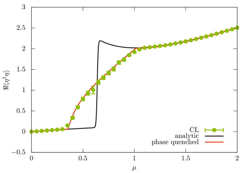
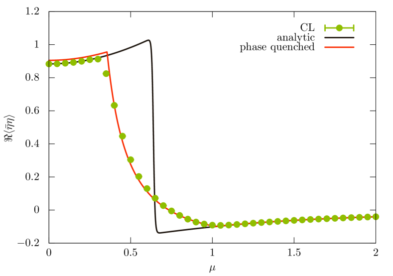
When employing the CL algorithm, the real degrees of freedom of the original model will take on complex values; this is called complexification. To clearly distinguish between pre- and post-complexification variables, we introduce the following notation,
| (9) |
where describes the RMT system before complexification, while and are general complex matrices describing the complexified system. At zero Langevin time, , we have , but this will no longer be the case for . In the Cartesian representation the complex matrices and are given by
| (10) |
where for , while for . As we already showed in conf16 a naive implementation of the algorithm leads to convergence to the phase quenched theory, as is clearly demonstrated in figure 1.
4 Gauge cooling
The RMT action is invariant under a gauge transformation, whereas after the variables have been complexified, this invariance is enhanced to a symmetry. One can utilize this additional gauge symmetry in order to modify the Langevin evolution in the hope to retrieve the correct results for this model. This method of treating the pathologies of the algorithm has been coined as gauge cooling, and has been employed with success on certain models sexty1 ; Nagata1 ; Nagata:2016mmh . Closely related to our study is its successful application to the Osborn model Nagata1 .
4.1 Cooling norms
The matrices , so that , are constructed in a way that reduces a cooling norm. Various norms are built in ways that parametrize pathological features of the Complex Langevin evolution. The natural norm is the Hermiticity norm which quantifies the difference between and ,
| (11) |
One can also introduce an eigenvalue norm Nagata1
| (12) |
where are the lowest eigenvalues of the positive definite matrix , and is a real positive parameter. Finally we can define an anti-Hermiticity norm which reads
| (13) |
The matrices and are the off-diagonal elements of : , . The first two norms as well as the anti-Hermiticity norm for were first proposed in Nagata1 . For the Stephanov model, we are using the anti-Hermiticity norm with because for the derivatives with respect to the similarity transformation are independent of the chemical potential. For the Osborn model, where this is not a problem, we use . Usually different norms attempt to fix different problems of the Langevin evolution so one can also combine them to make aggregate norms. For example one could combine the Hermiticity norm, which gives the magnitude of drift into the imaginary plane, with either the anti-Hermiticity or the eigenvalue norm, which both deal with the singularities of the drift,
| (14) |
We refer the reader to Nagata1 ; CLarticle for the details on how to construct the matrix .
4.2 Gauge cooling results
Next, we present our results when applying the method of gauge cooling to the two aforementioned matrix models. In these runs we have used a block matrix of size , Langevin stepsize , and runtime . Between each Langevin update we perform ten cooling transformations. In what follows the Stephanov model is simulated at parameters , while we chose for the Osborn model. Parameters are chosen in a way that the two models have a seemingly equally severe sign problem to overcome.
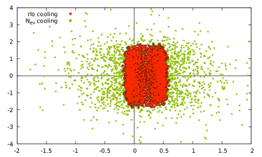
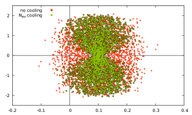
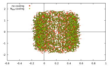
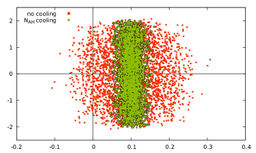
We start by looking at scatter plots of the eigenvalues of the Dirac matrix, shown in figure 2. In direct analogy with the results obtained by Nagata:2016mmh the RHS plot shows the effects of cooling on the Osborn model. For this model, the effect of cooling is that the eigenvalue distribution deforms and avoids the origin. On the other hand, this is not the case for the Stephanov model shown on the LHS. Figure 3 shows the same models cooled via . Here again, we observe that cooling cures the pathologies of the Osborn model but not of the Stephanov model.
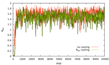
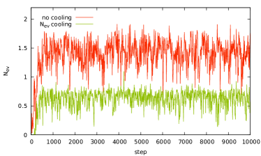
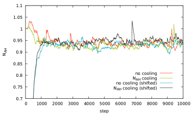
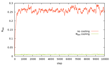
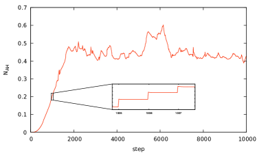
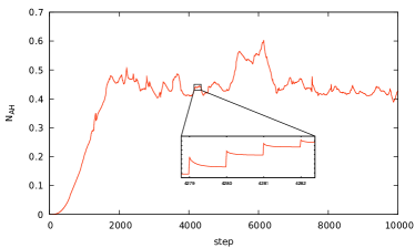
We now focus on (figure 4) and (figure 5) as a function of Langevin time. We observe that in the case of the Osborn model the norms are heavily reduced by the application of cooling but the Stephanov model is unaffected. Even in the extreme case of the shifted representation (see the next section), which through its advantageous initial conditions could have been a promising fix, we see that we obtain results similar to those without cooling and/or shifting. In figure 6 we show our results for matrices where we plot the norm and zoom in, in order to see better the effects of cooling and Langevin updates. Once thermalization has been reached we see that the cooling does not have a great enough impact on the simulation as to overcome a single Langevin update; this does not change when decreasing the CL algorithm’s stepsize, indicating that the solutions we are interested in are out of reach of the transformations.
5 Shifted representation
Another possible resolution of the problematic issues of the algorithm is to shift the chemical potential out of the fermion determinant to the "gauge" degrees of freedom. This can be achieved by a simple change of variables. The Dirac operator initially reads
| (15) |
One can absorb into as follows, . In terms of the matrices and the action reads
| (16) |
where and . This result in different Langevin forces CLarticle .
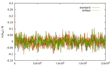
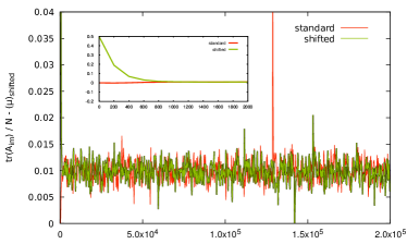
To analyze the dynamics of the shifted representation we analyze the matrix elements of and during a typical CL simulation; these are shown in figure 7. Although the two matrices start out very different, they do coincide after thermalization. This means that
| (17) |
and thus they converge to the same solution.
6 Conclusions
In this contribution we have performed a detailed comparison of the effects of gauge cooling on two different matrix models for QCD at finite density. We have shown that gauge cooling can fix the pathologies of the Osborn model, where the sign problem is artificial and can even be removed by careful redefinition of the parameters, but fails to overcome the problems of the Stephanov model which is a true matrix model for QCD at finite baryon density. The Stephanov model, possessing a phase transition to a phase with non-zero baryon density, is an excellent candidate for this type of investigations since dedicated studies have shown that CL fails when one approaches the deconfinement transition region of the QCD phase diagram, cf. Fodor and Bloch17 for an attempt to fix this problem.
7 Acknowledgements
SZ acknowledges support by the National Science Foundation (USA) under grant PHY-1516509 and by the Jefferson Science Associates, LLC under U.S. DOE Contract # DE-AC05- 06OR23177. JV acknowledges partial support from U.S. DOE Grant No. DEFAG- 88FR40388. JB was supported by the Deutsche Forschungsgemeinschaft (SFB/TRR-55). The authors would like to thank G. Aarts, I. O. Stamatescu, K. Nagata and J. Nishimura for fruitful discussions.
References
- (1) G. Parisi, Phys. Lett. 131B, 393 (1983)
- (2) G. Aarts, Phys. Rev. Lett. 102, 131601 (2009), 0810.2089
- (3) E. Seiler, 1708.08254
- (4) A.D. Jackson, J.J.M. Verbaarschot, Phys. Rev. D53, 7223 (1996)
- (5) M.A. Stephanov, Phys. Rev. Lett. 76, 4472 (1996)
- (6) P.H. Damgaard, K. Splittorff, J.J.M. Verbaarschot, Phys. Rev. Lett. 105, 162002 (2010)
- (7) G. Akemann, P.H. Damgaard, K. Splittorff, J.J.M. Verbaarschot, Phys. Rev. D83, 085014 (2011)
- (8) M. Kieburg, J.J.M. Verbaarschot, S. Zafeiropoulos, Phys. Rev. Lett. 108, 022001 (2012)
- (9) M. Kieburg, J.J.M. Verbaarschot, S. Zafeiropoulos, Phys. Rev. D88, 094502 (2013)
- (10) M. Kieburg, J.J.M. Verbaarschot, S. Zafeiropoulos, Phys. Rev. D92, 045026 (2015)
- (11) K. Cichy, K. Splittorff, S. Zafeiropoulos (2016), 1612.01289
- (12) A.M. Halasz, A.D. Jackson, R.E. Shrock, M.A. Stephanov, J.J.M. Verbaarschot, Phys. Rev. D58, 096007 (1998)
- (13) J.B. Kogut, M.A. Stephanov, D. Toublan, J.J.M. Verbaarschot, A. Zhitnitsky, Nucl. Phys. B582, 477 (2000)
- (14) J. Bloch, J. Glesaaen, O. Philipsen, J. Verbaarschot, S. Zafeiropoulos, EPJ Web Conf. 137, 07030 (2017)
- (15) E.V. Shuryak, J.J.M. Verbaarschot, Nucl. Phys. A560, 306 (1993)
- (16) J.C. Osborn, Phys. Rev. Lett. 93, 222001 (2004)
- (17) J. Bloch, Phys. Rev. D86, 074505 (2012)
- (18) A.M. Halasz, A.D. Jackson, J.J.M. Verbaarschot, Phys. Rev. D56, 5140 (1997)
- (19) E. Seiler, D. Sexty, I.O. Stamatescu, Phys. Lett. B723, 213 (2013)
- (20) K. Nagata, J. Nishimura, S. Shimasaki, JHEP 07, 073 (2016)
- (21) K. Nagata, H. Matsufuru, J. Nishimura, S. Shimasaki, PoS LATTICE2016, 067 (2016)
- (22) J. Bloch, J. Glesaaen, J.J.M. Verbaarschot, S. Zafeiropoulos (2017), 1712.07514
- (23) Z. Fodor, S.D. Katz, D. Sexty, C. TÃrÃk, Phys. Rev. D92, 094516 (2015)
- (24) J. Bloch, O. Schenk, 1707.08874