System-Aware Compression

Yehuda Dar, Michael Elad, and Alfred M. Bruckstein Computer Science Department, Technion – Israel Institute of Technology
{ydar,elad,freddy}@cs.technion.ac.il
Abstract

Many information systems employ lossy compression as a crucial intermediate stage among other processing components. While the important distortion is defined by the system’s input and output signals, the compression usually ignores the system structure, therefore, leading to an overall sub-optimal rate-distortion performance. In this paper we propose a compression methodology for an operational rate-distortion optimization considering a known system layout, modeled using linear operators and noise. Using the alternating direction method of multipliers (ADMM) technique, we show that the design of the new globally-optimized compression reduces to a standard compression of a ”system adjusted” signal. Essentially, the proposed framework leverages standard compression techniques to address practical settings of the noisy source coding problem. We further explain the main ideas of our method by theoretically studying the case of a cyclo-stationary Gaussian signal. We present experimental results for coding of one-dimensional signals and for video compression using the HEVC standard, showing significant gains by the adjustment to an acquisition-rendering system.

I Introduction

Lossy compression has a central role in information systems where the data may be inaccurately represented in order to meet storage-space or transmission-bandwidth constraints. While the compression is a crucial system-component, it is only an intermediate stage among data processing procedures that determine the eventual output of the system. For example, consider a common audio/visual system structure where the source signal is acquired and compressed for its storage/transmission, then the decompression is followed by a rendering stage producing the ultimate system output. Evidently, in this example, the quality of the system output is determined by the acquisition-rendering chain, and not solely on the lossy compression stage. Nevertheless, the compression is usually designed independently of the system structure, thus inducing a sub-optimal rate-distortion performance for the complete system.

Here we propose a compression approach defined by an operational rate-distortion optimization considering a known system structure. Specifically, we study a general flow (Fig. 1) where the compression is preceded by a linear operator distorting the input along with an additive white noise, and the decompression is followed by another linear operation. We formulate a rate-distortion optimization based on a quadratic distortion metric involving the system’s linear operators. For general linear operators, this intricate rate-distortion optimization is too hard to be directly solved for high dimensional signals. Consequently, we address this challenge using the alternating direction method of multipliers (ADMM) technique [1], suggesting an iterative procedure that relies on the simpler tasks of standard compression (which is system independent!) and 2subscript2\ell_{2}-constrained deconvolution for the linear operators of the system.

Refer to caption
Figure 1: The general system structure considered in this paper.

Optimizing the system output quality from the compression standpoint is an attractive answer to the inherent tradeoff among distortion, bit-cost, and computational complexity. First, bits are wisely spent for representing signal components that will be important at the output of the overall system (for example, one should obviously not code signal components belonging to the null space of the post-decompression operator). Second, the added computational load can be well accommodated in the compression environment that is often rich in computational and time resources, in contrast to the decompression stage.

Importantly, the proposed compression framework is a paradigm for addressing intricate rate-distortion optimization forms via iterative solution of easier problems emerging from the ADMM method (or other variable-splitting optimization techniques [2]). Indeed, the problem addressed here is an extension of our recent compression method [3] that pre-compensates for a later degradation occurring after decompression. In this paper the task is harder than in [3], as the source signal is available only in its degraded version. The recent wide use of ADMM for complicated signal restoration problems (e.g., [4, 5, 6, 7, 8]) suggests that our ADMM-based approach for complicated compression problems entails great potential.

Essentially, we study here a remote source coding problem (e.g., see its origins in [9, 10] and their successors). Our contribution is mainly the deterministic setting versus the statistical perspective used in previous works. Specifically, we consider an operational rate-distortion problem for the compression of a given signal, based on a different distortion metric imposed by the lack of an explicit statistical model of the unknown source. Our settings lead to the remarkable result that, using the ADMM technique, one can employ a standard compression method to address remote source coding problems in much more complicated instances than were previously feasible (e.g., [11]).

Using rate-distortion theory, we further study the examined problem in statistical settings (considering the proposed distortion metric) for the case of a cyclo-stationary Gaussian source signal and linear shift-invariant system operators. Our results show that the initial rate-distortion optimization reduces to a reverse water-filling procedure adjusted to the system operators and considering the pseudoinverse-filtered version of the input signal. We use these theoretic results to explain concepts appearing (differently) in the proposed practical method intended for non-Gaussian signals and general linear system operators.

Jointly using sampling and source coding procedures is fundamental to digitization-based systems (see, e.g., [12]). Accordingly, we demonstrate our general framework for adapting standard compression methods to the specific settings of a complete acquisition-rendering system. We present experiments considering coding of one-dimensional signals using an adaptive tree-based technique, and to video compression using the state-of-the-art HEVC standard [13]. Comparisons of our strategy to a regular compression flow exhibited that our method achieves significant gains at medium/high bit-rates.

II The Proposed Method

Let us describe the considered system structure (Fig. 1). A source signal, an N𝑁N-length column vector 𝐱N𝐱superscript𝑁\mathbf{x}\in\mathbb{R}^{N}, undergoes a linear processing represented by the M×N𝑀𝑁M\times N matrix 𝐀𝐀\mathbf{A} and, then, deteriorated by an additive white Gaussian noise vector 𝐧𝒩(0,σn2𝐈)similar-to𝐧𝒩0superscriptsubscript𝜎𝑛2𝐈\mathbf{n}\sim\mathcal{N}\left(0,\sigma_{n}^{2}\mathbf{I}\right), resulting in the signal

𝐰=𝐀𝐱+𝐧𝐰𝐀𝐱𝐧\displaystyle\mathbf{w}=\mathbf{A}\mathbf{x}+\mathbf{n} (1)

where 𝐰𝐰\mathbf{w} and 𝐧𝐧\mathbf{n} are M𝑀M-length column vectors. We represent the lossy compression procedure via the mapping C:M:𝐶superscript𝑀C:\mathbb{R}^{M}\rightarrow\mathcal{B} from the M𝑀M-dimensional signal domain to a discrete set \mathcal{B} of binary compressed representations (that may have different lengths). The signal 𝐰𝐰\mathbf{w} is the input to the compression component of the system, producing the compressed binary data b=C(𝐰)b𝐶𝐰\textit{b}=C\left(\mathbf{w}\right) that can be stored or transmitted in an error-free manner. Then, on a device and settings depending on the specific application, the compressed data bb\textit{b}\in\mathcal{B} is decompressed to provide the signal 𝐯=F(b)𝐯𝐹b\mathbf{v}=F\left(\textit{b}\right) where F:𝒮:𝐹𝒮F:\mathcal{B}\rightarrow\mathcal{S} represents the decompression mapping between the binary compressed representations in \mathcal{B} to the corresponding decompressed signals in the discrete set 𝒮M𝒮superscript𝑀\mathcal{S}\subset\mathbb{R}^{M}. The decompressed signal 𝐯𝐯\mathbf{v} is further processed by the linear operator denoted as the N×M𝑁𝑀N\times M matrix 𝐁𝐁\mathbf{B}, resulting in the system output signal

𝐲=𝐁𝐯,𝐲𝐁𝐯\displaystyle\mathbf{y}=\mathbf{B}\mathbf{v}, (2)

which is an N𝑁N-length real-valued column vector.

As an example, consider an acquisition-compression-rendering system where the signal 𝐰𝐰\mathbf{w} is a sampled version of the source signal 𝐱𝐱\mathbf{x}, and the system output 𝐲𝐲\mathbf{y} is the rendered version of the decompressed signal 𝐯𝐯\mathbf{v}.

We assume here that the operators 𝐀𝐀\mathbf{A} and 𝐁𝐁\mathbf{B}, as well as the noise variance σn2superscriptsubscript𝜎𝑛2\sigma_{n}^{2}, are known and fixed (i.e., cannot be optimized). Consequently, we formulate a new compression procedure in order to optimize the end-to-end rate-distortion performance of the entire system. Specifically, we want the system output 𝐲𝐲\mathbf{y} to be the best approximation of the source signal 𝐱𝐱\mathbf{x} under the bit-budget constraint. However, at the compression stage we do not accurately know 𝐱𝐱\mathbf{x}, but rather its degraded form 𝐰𝐰\mathbf{w} formulated in (1). This motivates us to suggest the following distortion metric with respect to the system output 𝐲𝐲\mathbf{y}

ds(𝐰,𝐲)=1M𝐰𝐀𝐲22.subscript𝑑𝑠𝐰𝐲1𝑀superscriptsubscriptnorm𝐰𝐀𝐲22\displaystyle d_{s}\left(\mathbf{w},\mathbf{y}\right)=\frac{1}{M}\left\|{\mathbf{w}-\mathbf{A}\mathbf{y}}\right\|_{2}^{2}. (3)

This metric conforms with the fact that if 𝐲𝐲\mathbf{y} is close to 𝐱𝐱\mathbf{x}, then, by (1), 𝐰𝐰\mathbf{w} will be close to 𝐀𝐲𝐀𝐲\mathbf{A}\mathbf{y} up to the noise 𝐧𝐧\mathbf{n}. Indeed, for the ideal case of 𝐲=𝐱𝐲𝐱\mathbf{y}=\mathbf{x} the metric (3) becomes

ds(𝐰,𝐱)=1M𝐧22σn2subscript𝑑𝑠𝐰𝐱1𝑀superscriptsubscriptnorm𝐧22superscriptsubscript𝜎𝑛2\displaystyle d_{s}\left(\mathbf{w},\mathbf{x}\right)=\frac{1}{M}\left\|{\mathbf{n}}\right\|_{2}^{2}\approx\sigma_{n}^{2} (4)

where the last approximate equality is under the assumption of a sufficiently large M𝑀M (the length of 𝐧𝐧\mathbf{n}). Since 𝐲=𝐁𝐯𝐲𝐁𝐯\mathbf{y}=\mathbf{B}\mathbf{v}, we can rewrite the distortion ds(𝐰,𝐲)subscript𝑑𝑠𝐰𝐲d_{s}\left(\mathbf{w},\mathbf{y}\right) in (3) as a function of the decompressed signal 𝐯𝐯\mathbf{v}, namely,

dc(𝐰,𝐯)=1M𝐰𝐀𝐁𝐯22.subscript𝑑𝑐𝐰𝐯1𝑀superscriptsubscriptnorm𝐰𝐀𝐁𝐯22\displaystyle d_{c}\left(\mathbf{w},\mathbf{v}\right)=\frac{1}{M}\left\|{\mathbf{w}-\mathbf{A}\mathbf{B}\mathbf{v}}\right\|_{2}^{2}. (5)

Since the operator 𝐁𝐁\mathbf{B} produces the output signal 𝐲𝐲\mathbf{y}, an ideal result will be 𝐲=𝐏B𝐱𝐲subscript𝐏𝐵𝐱\mathbf{y}=\mathbf{P}_{B}\mathbf{x}, where 𝐏Bsubscript𝐏𝐵\mathbf{P}_{B} is the matrix projecting onto 𝐁𝐁\mathbf{B}’s range. The corresponding ideal distortion is

D0ds(𝐰,𝐏B𝐱)=1M𝐀(𝐈𝐏B)𝐱+𝐧22.subscript𝐷0subscript𝑑𝑠𝐰subscript𝐏𝐵𝐱1𝑀superscriptsubscriptnorm𝐀𝐈subscript𝐏𝐵𝐱𝐧22\displaystyle D_{0}\triangleq d_{s}\left(\mathbf{w},\mathbf{P}_{B}\mathbf{x}\right)=\frac{1}{M}\left\|{\mathbf{A}\left(\mathbf{I}-\mathbf{P}_{B}\right)\mathbf{x}+\mathbf{n}}\right\|_{2}^{2}. (6)

We use the distortion metric (5) to constrain the bit-cost minimization in the following rate-distortion optimization

𝐯^=argmin𝐯𝒮R(𝐯)subject toD01M𝐰𝐀𝐁𝐯22D0+Dmissing-subexpression^𝐯𝐯𝒮argminmissing-subexpression𝑅𝐯missing-subexpressionsubject tomissing-subexpressionsubscript𝐷01𝑀superscriptsubscriptnorm𝐰𝐀𝐁𝐯22subscript𝐷0𝐷\displaystyle\begin{aligned} &\hat{\mathbf{v}}=\underset{\mathbf{v}\in\mathcal{S}}{\text{argmin}}&&{R\left(\mathbf{v}\right)}\\ &\text{subject to}&&D_{0}\leq\frac{1}{M}\left\|{\mathbf{w}-\mathbf{A}\mathbf{B}\mathbf{v}}\right\|_{2}^{2}\leq D_{0}+D\end{aligned} (7)

where R(𝐯)𝑅𝐯R\left(\mathbf{v}\right) evaluates the length of the binary compressed description of the decompressed signal 𝐯𝐯\mathbf{v}, and D0𝐷0D\geq 0 determines the allowed distortion. By (6), the value D0subscript𝐷0D_{0} depends on the operator 𝐀𝐀\mathbf{A}, the null space of 𝐁𝐁\mathbf{B}, the source signal 𝐱𝐱\mathbf{x}, and the noise realization 𝐧𝐧\mathbf{n}. Since 𝐱𝐱\mathbf{x} and 𝐧𝐧\mathbf{n} are unknown, D0subscript𝐷0D_{0} cannot be accurately calculated in the operational case (in Section III we formulate the expected value of D0subscript𝐷0D_{0} for the case of a cyclo-stationary Gaussian source signal). We address the optimization (7) using its unconstrained Lagrangian form

𝐯^=argmin𝐯𝒮R(𝐯)+λ1M𝐰𝐀𝐁𝐯22^𝐯𝐯𝒮argmin𝑅𝐯𝜆1𝑀superscriptsubscriptnorm𝐰𝐀𝐁𝐯22\displaystyle\hat{\mathbf{v}}=\underset{\mathbf{v}\in\mathcal{S}}{\text{argmin}}~{}~{}{R\left(\mathbf{v}\right)+\lambda\frac{1}{M}\left\|{\mathbf{w}-\mathbf{A}\mathbf{B}\mathbf{v}}\right\|_{2}^{2}} (8)

where λ0𝜆0\lambda\geq 0 is a Lagrange multiplier corresponding to some distortion constraint DλD0subscript𝐷𝜆subscript𝐷0D_{\lambda}\geq D_{0} (such optimization strategy with respect to some Lagrange multiplier is common, e.g., in video coding [13]). In the case of high-dimensional signals, the discrete set 𝒮𝒮\mathcal{S} is extremely large and, therefore, it is impractical to directly solve the Lagrangian form in (8) for generally structured matrices 𝐀𝐀\mathbf{A} and 𝐁𝐁\mathbf{B}. This difficulty vanishes, for example, when 𝐀=𝐁=𝐈𝐀𝐁𝐈\mathbf{A}=\mathbf{B}=\mathbf{I}, reducing the Lagrangian optimization in (8) to the standard (system independent) compression form (see, e.g., [14, 15]). Indeed, such standard Lagrangian rate-distortion optimizations are practically solved using block-based designs that translate the task to a sequence of block-level optimizations of feasible dimensions.

Here we consider general 𝐀𝐀\mathbf{A} and 𝐁𝐁\mathbf{B} matrices, and address the computational difficulty in solving (8) using the alternating direction method of multipliers (ADMM) technique [1]. For start, we apply variable splitting to rewrite (8) as

𝐯^=argmin𝐯𝒮,𝐳MR(𝐯)+λ1M𝐰𝐀𝐁𝐳22subject to𝐯=𝐳missing-subexpression^𝐯formulae-sequence𝐯𝒮𝐳superscript𝑀argmin𝑅𝐯𝜆1𝑀superscriptsubscriptnorm𝐰𝐀𝐁𝐳22missing-subexpressionsubject to𝐯𝐳\displaystyle\begin{aligned} &\hat{\mathbf{v}}=\underset{\mathbf{v}\in\mathcal{S},{\mathbf{z}}\in\mathbb{R}^{M}}{\text{argmin}}~{}~{}{R\left(\mathbf{v}\right)+\lambda\frac{1}{M}\left\|{\mathbf{w}-\mathbf{A}\mathbf{B}\mathbf{z}}\right\|_{2}^{2}}\\ &\text{subject to}~{}~{}~{}~{}\mathbf{v}=\mathbf{z}\end{aligned} (9)

where 𝐳M𝐳superscript𝑀\mathbf{z}\in\mathbb{R}^{M} is an auxiliary variable that is not (directly) restricted to the discrete set 𝒮𝒮\mathcal{S}. The augmented Lagrangian (in its scaled form) and the method of multipliers (see [1, Ch. 2]) turn (9) into the following iterative procedure

(𝐯^(t),𝐳^(t))=superscript^𝐯𝑡superscript^𝐳𝑡absent\displaystyle\left(\hat{\mathbf{v}}^{(t)},\hat{\mathbf{z}}^{(t)}\right)= (10)
argmin𝐯𝒮,𝐳MR(𝐯)+λ1M𝐰𝐀𝐁𝐳22+β2𝐯𝐳+𝐮(t)22subscriptargminformulae-sequence𝐯𝒮𝐳superscript𝑀𝑅𝐯𝜆1𝑀superscriptsubscriptnorm𝐰𝐀𝐁𝐳22𝛽2superscriptsubscriptnorm𝐯𝐳superscript𝐮𝑡22\displaystyle\mathop{{\text{argmin}}}\limits_{\mathbf{v}\in\mathcal{S},{\mathbf{z}}\in\mathbb{R}^{M}}R\left(\mathbf{v}\right)+\lambda\frac{1}{M}\left\|{\mathbf{w}-\mathbf{A}\mathbf{B}\mathbf{z}}\right\|_{2}^{2}+\frac{\beta}{2}{\left\|{\mathbf{v}-\mathbf{z}+\mathbf{u}^{(t)}}\right\|_{2}^{2}}
𝐮(t+1)=𝐮(t)+(𝐯^(t)𝐳^(t)),superscript𝐮𝑡1superscript𝐮𝑡superscript^𝐯𝑡superscript^𝐳𝑡\displaystyle\mathbf{u}^{(t+1)}=\mathbf{u}^{(t)}+\left(\hat{\mathbf{v}}^{(t)}-\hat{\mathbf{z}}^{(t)}\right), (11)

where t𝑡t is the iteration number, 𝐮(t)Msuperscript𝐮𝑡superscript𝑀\mathbf{u}^{(t)}\in\mathbb{R}^{M} is the scaled dual variable, and β𝛽\beta is an auxiliary parameter originating at the augmented Lagrangian. Further simplifying (10) using one iteration of alternating minimization gives the ADMM form of the problem

𝐯^(t)=argmin𝐯𝒮R(𝐯)+β2𝐯𝐳~(t)22superscript^𝐯𝑡subscriptargmin𝐯𝒮𝑅𝐯𝛽2superscriptsubscriptnorm𝐯superscript~𝐳𝑡22\displaystyle\hat{\mathbf{v}}^{(t)}=\mathop{{\text{argmin}}}\limits_{\mathbf{v}\in\mathcal{S}}R\left(\mathbf{v}\right)+\frac{\beta}{2}{\left\|{\mathbf{v}-\tilde{\mathbf{z}}^{(t)}}\right\|_{2}^{2}} (12)
𝐳^(t)=argmin𝐳Mλ1M𝐰𝐀𝐁𝐳22+β2𝐳𝐯~(t)22superscript^𝐳𝑡subscriptargmin𝐳superscript𝑀𝜆1𝑀superscriptsubscriptnorm𝐰𝐀𝐁𝐳22𝛽2superscriptsubscriptnorm𝐳superscript~𝐯𝑡22\displaystyle\hat{\mathbf{z}}^{(t)}=\mathop{\text{argmin}}\limits_{{\mathbf{z}}\in\mathbb{R}^{M}}\lambda\frac{1}{M}\left\|{\mathbf{w}-\mathbf{A}\mathbf{B}\mathbf{z}}\right\|_{2}^{2}+\frac{\beta}{2}{\left\|{\mathbf{z}-\tilde{\mathbf{v}}^{(t)}}\right\|_{2}^{2}} (13)
𝐮(t+1)=𝐮(t)+(𝐯^(t)𝐳^(t)).superscript𝐮𝑡1superscript𝐮𝑡superscript^𝐯𝑡superscript^𝐳𝑡\displaystyle\mathbf{u}^{(t+1)}=\mathbf{u}^{(t)}+\left(\hat{\mathbf{v}}^{(t)}-\hat{\mathbf{z}}^{(t)}\right). (14)

where 𝐳~(t)=𝐳^(t1)𝐮(t)superscript~𝐳𝑡superscript^𝐳𝑡1superscript𝐮𝑡\tilde{\mathbf{z}}^{(t)}=\hat{\mathbf{z}}^{(t-1)}-\mathbf{u}^{(t)} and 𝐯~(t)=𝐯^(t)+𝐮(t)superscript~𝐯𝑡superscript^𝐯𝑡superscript𝐮𝑡\tilde{\mathbf{v}}^{(t)}=\hat{\mathbf{v}}^{(t)}+\mathbf{u}^{(t)}. Importantly, the compression design, expressed by {𝒮,R}𝒮𝑅\left\{\mathcal{S},R\right\}, and the system-specific operators {𝐀,𝐁}𝐀𝐁\left\{\mathbf{A},\mathbf{B}\right\} were decoupled by the ADMM to reside in distinct optimization problems that are easier to solve.

We identify the first stage (12) as the Lagrangian optimization employed for standard compression (and decompression) tasks considering the regular mean squared error metric. Specifically, the Lagrange multiplier for this standard optimization is λ~=βM2~𝜆𝛽𝑀2\tilde{\lambda}=\frac{\beta M}{2}. Furthermore, we suggest to replace the solution of (12) with the application of a standard compression (and decompression) technique, even one that does not follow the Lagrangian optimization formulated in (12). We denote the standard compression and decompression via

b(t)=StandardCompress(𝐳~(t),θ)superscriptb𝑡𝑆𝑡𝑎𝑛𝑑𝑎𝑟𝑑𝐶𝑜𝑚𝑝𝑟𝑒𝑠𝑠superscript~𝐳𝑡𝜃\displaystyle{\textit{b}}^{(t)}=StandardCompress\left(\tilde{\mathbf{z}}^{(t)},\theta\right) (15)
𝐯^(t)=StandardDecompress(b(t))superscript^𝐯𝑡𝑆𝑡𝑎𝑛𝑑𝑎𝑟𝑑𝐷𝑒𝑐𝑜𝑚𝑝𝑟𝑒𝑠𝑠superscriptb𝑡\displaystyle\hat{\mathbf{v}}^{(t)}=StandardDecompress\left({\textit{b}}^{(t)}\right) (16)

where θ𝜃\theta is a general parameter that extends the Lagrange multiplier role in determining the rate-distortion tradeoff (see Algorithm 1). This important suggestion defines our method as a generic approach that can optimize any compression technique with respect to the specific system it resides in.

The second optimization stage (13) is an 2subscript2\ell_{2}-constrained deconvolution problem, that can be easily solved in various ways. The analytic solution of (13) is

𝐳^(t)=(𝐁𝐀𝐀𝐁+βM2λ𝐈)1(𝐁𝐀𝐰+βM2λ𝐯~(t)),superscript^𝐳𝑡superscriptsuperscript𝐁superscript𝐀𝐀𝐁𝛽𝑀2𝜆𝐈1superscript𝐁superscript𝐀𝐰𝛽𝑀2𝜆superscript~𝐯𝑡\displaystyle\hat{\mathbf{z}}^{(t)}=\left(\mathbf{B}^{*}\mathbf{A}^{*}\mathbf{A}\mathbf{B}+\frac{\beta M}{2\lambda}\mathbf{I}\right)^{-1}\left(\mathbf{B}^{*}\mathbf{A}^{*}\mathbf{w}+\frac{\beta M}{2\lambda}\tilde{\mathbf{v}}^{(t)}\right),~{}~{}~{} (17)

showing it as a weighted averaging of 𝐰𝐰\mathbf{w} and 𝐯~(t)superscript~𝐯𝑡\tilde{\mathbf{v}}^{(t)}. In the generic description given in Algorithm 1 we replace the quantity βM2λ𝛽𝑀2𝜆\frac{\beta M}{2\lambda} with the parameter β~~𝛽\tilde{\beta}.

The proposed method is summarized in Algorithm 1. Our goal is to provide a binary compressed representation of the optimized solution. Hence, the procedure output is the compressed data, b(t)superscriptb𝑡{\textit{b}}^{(t)}, obtained in the compression stage of the last iteration.

Algorithm 1 Generic System-Aware Compression
1:Inputs: 𝐰𝐰\mathbf{w}, θ𝜃\theta, β~~𝛽\tilde{\beta}.
2:Initialize t=0𝑡0t=0 , 𝐳^(0)=𝐰superscript^𝐳0𝐰{\hat{\mathbf{z}}}^{(0)}=\mathbf{w} , 𝐮(1)=𝟎superscript𝐮10\mathbf{u}^{(1)}=\mathbf{0}.
3:repeat
4:     tt+1𝑡𝑡1t\leftarrow t+1
5:     𝐳~(t)=𝐳^(t1)𝐮(t)superscript~𝐳𝑡superscript^𝐳𝑡1superscript𝐮𝑡\tilde{\mathbf{z}}^{(t)}=\hat{\mathbf{z}}^{(t-1)}-\mathbf{u}^{(t)}
6:     b(t)=StandardCompress(𝐳~(t),θ)superscriptb𝑡𝑆𝑡𝑎𝑛𝑑𝑎𝑟𝑑𝐶𝑜𝑚𝑝𝑟𝑒𝑠𝑠superscript~𝐳𝑡𝜃{\textit{b}}^{(t)}=StandardCompress\left(\tilde{\mathbf{z}}^{(t)},\theta\right)
7:     𝐯^(t)=StandardDecompress(b(t))superscript^𝐯𝑡𝑆𝑡𝑎𝑛𝑑𝑎𝑟𝑑𝐷𝑒𝑐𝑜𝑚𝑝𝑟𝑒𝑠𝑠superscriptb𝑡\hat{\mathbf{v}}^{(t)}=StandardDecompress\left({\textit{b}}^{(t)}\right)
8:     𝐯~(t)=𝐯^(t)+𝐮(t)superscript~𝐯𝑡superscript^𝐯𝑡superscript𝐮𝑡\tilde{\mathbf{v}}^{(t)}=\hat{\mathbf{v}}^{(t)}+\mathbf{u}^{(t)}
9:     𝐳^(t)=(𝐁𝐀𝐀𝐁+β~𝐈)1(𝐁𝐀𝐰+β~𝐯~(t))superscript^𝐳𝑡superscriptsuperscript𝐁superscript𝐀𝐀𝐁~𝛽𝐈1superscript𝐁superscript𝐀𝐰~𝛽superscript~𝐯𝑡\hat{\mathbf{z}}^{(t)}=\left(\mathbf{B}^{*}\mathbf{A}^{*}\mathbf{A}\mathbf{B}+\tilde{\beta}\mathbf{I}\right)^{-1}\left(\mathbf{B}^{*}\mathbf{A}^{*}\mathbf{w}+\tilde{\beta}\tilde{\mathbf{v}}^{(t)}\right)
10:     𝐮(t+1)=𝐮(t)+(𝐯^(t)𝐳^(t))superscript𝐮𝑡1superscript𝐮𝑡superscript^𝐯𝑡superscript^𝐳𝑡\mathbf{u}^{(t+1)}=\mathbf{u}^{(t)}+\left(\hat{\mathbf{v}}^{(t)}-\hat{\mathbf{z}}^{(t)}\right)
11:until stopping criterion is satisfied
12:Output: b(t)superscriptb𝑡{\textit{b}}^{(t)}, which is the binary compressed data obtained in the last iteration.

III Theoretic Analysis for the Gaussian Case

In this section we use the rate-distortion theory framework to further explore the fundamental problem of system-optimized compression. We consider the case of a cyclo-stationary Gaussian signal and system involving linear shift-invariant operators and no noise, yet, the obtained results exhibit the prominent ideas of the general problem and the operational method presented in Section II.

III-A Problem Formulation and Solution

The source signal is modeled here as 𝐱𝒩(0,𝐑𝐱)similar-to𝐱𝒩0subscript𝐑𝐱\mathbf{x}\sim\mathcal{N}\left(0,\mathbf{R}_{\mathbf{x}}\right), i.e., a zero-mean Gaussian random vector with a circulant autocorrelation matrix 𝐑𝐱subscript𝐑𝐱\mathbf{R}_{\mathbf{x}}. The eigenvalues of 𝐑𝐱subscript𝐑𝐱\mathbf{R}_{\mathbf{x}} are denoted as {λk(𝐱)}k=0N1superscriptsubscriptsuperscriptsubscript𝜆𝑘𝐱𝑘0𝑁1\left\{\lambda_{k}^{\left(\mathbf{x}\right)}\right\}_{k=0}^{N-1}. The first processing part of the system produces the signal 𝐰=𝐀𝐱𝐰𝐀𝐱{\mathbf{w}}=\mathbf{A}\mathbf{x}, where here 𝐀𝐀\mathbf{A} is a real-valued N×N𝑁𝑁N\times N circulant matrix. Evidently, the signal 𝐰𝐰\mathbf{w} is a zero-mean Gaussian random vector with autocorrelation matrix 𝐑𝐰=𝐀𝐑𝐱𝐀subscript𝐑𝐰subscript𝐀𝐑𝐱superscript𝐀\mathbf{R}_{\mathbf{w}}\nolinebreak=\nolinebreak\mathbf{A}\mathbf{R}_{\mathbf{x}}\mathbf{A}^{*}.

Here 𝐀𝐀\mathbf{A} and 𝐁𝐁\mathbf{B} are circulant N×N𝑁𝑁N\times N matrices, thus, diagonalized by the N×N𝑁𝑁N\times N Discrete Fourier Transform (DFT) matrix 𝐅𝐅\mathbf{F} as 𝐅𝐀𝐅=𝚲𝐀superscript𝐅𝐀𝐅subscript𝚲𝐀\mathbf{F}\mathbf{A}\mathbf{F}^{*}=\mathbf{\Lambda}_{\mathbf{A}} and 𝐅𝐁𝐅=𝚲𝐁superscript𝐅𝐁𝐅subscript𝚲𝐁\mathbf{F}\mathbf{B}\mathbf{F}^{*}=\mathbf{\Lambda}_{\mathbf{B}}, where 𝚲𝐀subscript𝚲𝐀\mathbf{\Lambda}_{\mathbf{A}} and 𝚲𝐁subscript𝚲𝐁\mathbf{\Lambda}_{\mathbf{B}} are diagonal matrices formed by the elements {akF}k=0N1superscriptsubscriptsubscriptsuperscript𝑎𝐹𝑘𝑘0𝑁1\left\{a^{F}_{k}\right\}_{k=0}^{N-1} and {bkF}k=0N1superscriptsubscriptsubscriptsuperscript𝑏𝐹𝑘𝑘0𝑁1\left\{b^{F}_{k}\right\}_{k=0}^{N-1}, respectively. Accordingly, the pseudoinverse matrix of 𝐀𝐀\mathbf{A} is defined as 𝐀+=𝐅𝚲𝐀+𝐅superscript𝐀superscript𝐅superscriptsubscript𝚲𝐀𝐅\mathbf{A}^{+}=\mathbf{F}^{*}\mathbf{\Lambda}_{\mathbf{A}}^{+}\mathbf{F}, where 𝚲𝐀+superscriptsubscript𝚲𝐀\mathbf{\Lambda}_{\mathbf{A}}^{+} is the pseudoinverse of 𝚲𝐀subscript𝚲𝐀\mathbf{\Lambda}_{\mathbf{A}}, an N×N𝑁𝑁N\times N diagonal matrix with the kthsuperscript𝑘𝑡k^{th} diagonal component akF,+=1/akFsubscriptsuperscript𝑎𝐹𝑘1subscriptsuperscript𝑎𝐹𝑘a^{F,+}_{k}={1}/{a^{F}_{k}} for k𝑘k where akF0subscriptsuperscript𝑎𝐹𝑘0a^{F}_{k}\neq 0, and akF,+=0subscriptsuperscript𝑎𝐹𝑘0a^{F,+}_{k}=0 for k𝑘k where akF=0subscriptsuperscript𝑎𝐹𝑘0a^{F}_{k}=0. The matrix 𝐁𝐁\mathbf{B} has corresponding definitions to those given above for 𝐀𝐀\mathbf{A}.

Recall that the system output is 𝐲=𝐁𝐯𝐲𝐁𝐯\mathbf{y}=\mathbf{B}\mathbf{v}, where here 𝐯𝐯\mathbf{v} is the random vector representing the decompressed signal. Accordingly, in the theoretic framework here, the rate is associated with the mutual information I(𝐰,𝐲)𝐼𝐰𝐲I\left(\mathbf{w},\mathbf{y}\right). In (7) we formulated the operational rate-distortion optimization describing our practical task, cast here in the theoretic framework to

minp𝐯|𝐰I(𝐰;𝐁𝐯)s.t.NE{D0}E{𝐰𝐀𝐁𝐯22}N(E{D0}+D)missing-subexpressionsubscript𝑝conditional𝐯𝐰minmissing-subexpression𝐼𝐰𝐁𝐯missing-subexpressions.t.missing-subexpression𝑁𝐸subscript𝐷0𝐸superscriptsubscriptnorm𝐰𝐀𝐁𝐯22𝑁𝐸subscript𝐷0𝐷\displaystyle\begin{aligned} &\underset{p_{\mathbf{v}|\mathbf{w}}}{\text{min}}&&{I\left(\mathbf{w};\mathbf{B}\mathbf{v}\right)}\\ &\text{s.t.}&&NE\left\{D_{0}\right\}\leq E\left\{\left\|{\mathbf{w}-\mathbf{A}\mathbf{B}\mathbf{v}}\right\|_{2}^{2}\right\}\leq N\left(E\left\{D_{0}\right\}+D\right)\end{aligned} (18)

where p𝐯|𝐰subscript𝑝conditional𝐯𝐰p_{\mathbf{v}|\mathbf{w}} is the conditional probability-density-function of 𝐯𝐯\mathbf{v} given 𝐰𝐰\mathbf{w}, and D0𝐷0D\geq 0 determines the allowed expected distortion. The value E{D0}𝐸subscript𝐷0E\left\{D_{0}\right\}, stemming from (6) and the noiseless settings here, is the minimal expected distortion evaluated (see Appendix A) as

E{D0}=1Nk:akF0,bkF=0|akF|2λk(𝐱).𝐸subscript𝐷01𝑁subscript:𝑘formulae-sequencesuperscriptsubscript𝑎𝑘𝐹0superscriptsubscript𝑏𝑘𝐹0superscriptsuperscriptsubscript𝑎𝑘𝐹2superscriptsubscript𝜆𝑘𝐱\displaystyle E\left\{D_{0}\right\}=\frac{1}{N}\sum\limits_{k:a_{k}^{F}\neq 0~{},~{}b_{k}^{F}=0}{\left\lvert a_{k}^{F}\right\rvert^{2}\lambda_{k}^{\left(\mathbf{x}\right)}}. (19)

We state that the basic rate-distortion optimization problem in (18) is equivalent to (see proof in Appendix B)

minp𝐯|𝐰~I(𝐰~;𝐏𝐁𝐏𝐀𝐯)s.t.E{𝐀𝐁(𝐰~𝐯)22}NDmissing-subexpressionsubscript𝑝conditional𝐯~𝐰minmissing-subexpression𝐼~𝐰subscript𝐏𝐁subscript𝐏𝐀𝐯missing-subexpressions.t.missing-subexpression𝐸superscriptsubscriptnorm𝐀𝐁~𝐰𝐯22𝑁𝐷\displaystyle\begin{aligned} &\underset{p_{\mathbf{v}|\tilde{\mathbf{w}}}}{\text{min}}&&{I\left(\tilde{\mathbf{w}};\mathbf{P}_{\mathbf{B}}\mathbf{P}_{\mathbf{A}}\mathbf{v}\right)}\\ &\text{s.t.}&&E\left\{\left\|{\mathbf{A}\mathbf{B}\left(\tilde{\mathbf{w}}-\mathbf{v}\right)}\right\|_{2}^{2}\right\}\leq ND~{}~{}~{}~{}~{}\end{aligned} (20)

where 𝐰~=𝐁+𝐀+𝐰~𝐰superscript𝐁superscript𝐀𝐰{\tilde{\mathbf{w}}}=\mathbf{B}^{+}\mathbf{A}^{+}\mathbf{w} is the pseudoinverse filtered compression-input 𝐰𝐰\mathbf{w}. Here 𝐏𝐀subscript𝐏𝐀\mathbf{P}_{\mathbf{A}} and 𝐏𝐁subscript𝐏𝐁\mathbf{P}_{\mathbf{B}} are projection matrices corresponding to the range of 𝐀𝐀\mathbf{A} and 𝐁𝐁\mathbf{B}, respectively. We define the set 𝒦AB{k:akF0andbkF0}subscript𝒦𝐴𝐵conditional-set𝑘superscriptsubscript𝑎𝑘𝐹0andsuperscriptsubscript𝑏𝑘𝐹0\mathcal{K}_{AB}\nolinebreak\triangleq\nolinebreak\left\{k:a_{k}^{F}\neq 0~{}\text{and}~{}b_{k}^{F}\neq 0\right\} that contains the DFT-domain component indices belonging to the range of the joint operator 𝐀𝐁𝐀𝐁\mathbf{AB}.

Since 𝐰~~𝐰\tilde{\mathbf{w}} is a cyclo-stationary Gaussian random vector, we transform the optimization (20) into a Fourier-domain distortion-allocation problem considering independent Gaussian variables (see proof in Appendix C), namely,

min{Dk}k𝒦ABk𝒦AB12log(λk(𝐰~)Dk)s.t.k𝒦AB|akFbkF|2DkND0Dkλk(𝐰~),k𝒦AB.missing-subexpressionsubscriptsubscript𝐷𝑘𝑘subscript𝒦𝐴𝐵minmissing-subexpressionsubscript𝑘subscript𝒦𝐴𝐵12subscriptsuperscript𝜆~𝐰𝑘subscript𝐷𝑘missing-subexpressions.t.missing-subexpressionsubscript𝑘subscript𝒦𝐴𝐵superscriptsubscriptsuperscript𝑎𝐹𝑘subscriptsuperscript𝑏𝐹𝑘2subscript𝐷𝑘𝑁𝐷missing-subexpressionmissing-subexpressionmissing-subexpressionformulae-sequence0subscript𝐷𝑘subscriptsuperscript𝜆~𝐰𝑘𝑘subscript𝒦𝐴𝐵\displaystyle\begin{aligned} &\underset{\left\{D_{k}\right\}_{k\in\mathcal{K}_{AB}}}{\text{min}}&&\sum\limits_{k\in\mathcal{K}_{AB}}{\frac{1}{2}\log\left({\frac{\lambda^{\left(\tilde{\mathbf{w}}\right)}_{k}}{D_{k}}}\right)}\\ &\text{s.t.}&&\sum\limits_{k\in\mathcal{K}_{AB}}{\left|a^{F}_{k}b^{F}_{k}\right|^{2}D_{k}}\leq ND~{}~{}~{}\\ &&&0\leq D_{k}\leq\lambda^{\left(\tilde{\mathbf{w}}\right)}_{k}~{}~{}~{},~{}{k\in\mathcal{K}_{AB}}.\end{aligned} (21)

where for k𝒦AB𝑘subscript𝒦𝐴𝐵{k\in\mathcal{K}_{AB}} the value λk(𝐰~)=λk(𝐰)/|akFbkF|2subscriptsuperscript𝜆~𝐰𝑘subscriptsuperscript𝜆𝐰𝑘superscriptsubscriptsuperscript𝑎𝐹𝑘subscriptsuperscript𝑏𝐹𝑘2\lambda^{\left(\tilde{\mathbf{w}}\right)}_{k}=\lambda^{\left({\mathbf{w}}\right)}_{k}/{\left|a^{F}_{k}b^{F}_{k}\right|^{2}} is the variance of the kthsuperscript𝑘𝑡k^{th} DFT-coefficient of 𝐰~~𝐰{\tilde{\mathbf{w}}}. The solution of problem (21), obtained using Lagrangian optimization and the KKT conditions, is given by the following distortion allocation: for k𝒦AB𝑘subscript𝒦𝐴𝐵k\in\mathcal{K}_{AB}

Dk={θ/|akFbkF|2,for 0θ<|akFbkF|2λk(𝐰~)λk(𝐰~),for θ|akFbkF|2λk(𝐰~),\displaystyle D_{k}=\left\{{\begin{array}[]{*{20}{c}}{\theta/\left|a^{F}_{k}b^{F}_{k}\right|^{2}}&{,\text{for~{}~{}}0\leq\theta<\left|a^{F}_{k}b^{F}_{k}\right|^{2}\lambda^{\left(\tilde{\mathbf{w}}\right)}_{k}}\\ \lambda^{\left(\tilde{\mathbf{w}}\right)}_{k}&{,\text{for~{}~{}~{}}\theta\geq\left|a^{F}_{k}b^{F}_{k}\right|^{2}\lambda^{\left(\tilde{\mathbf{w}}\right)}_{k},}{}{}\end{array}}\right. (24)

where θ𝜃\theta is set such that k𝒦AB|akFbkF|2Dk=NDsubscript𝑘subscript𝒦𝐴𝐵superscriptsubscriptsuperscript𝑎𝐹𝑘subscriptsuperscript𝑏𝐹𝑘2subscript𝐷𝑘𝑁𝐷\sum\limits_{k\in\mathcal{K}_{AB}}{\left|a^{F}_{k}b^{F}_{k}\right|^{2}D_{k}}=ND is satisfied. Importantly, for k𝒦AB𝑘subscript𝒦𝐴𝐵k\notin\mathcal{K}_{AB} the rate is Rk=0subscript𝑅𝑘0R_{k}=0 and the distortion is set to Dk=0subscript𝐷𝑘0D_{k}=0 (see Appendix C). The optimal rates corresponding to (24) assign for k𝒦AB𝑘subscript𝒦𝐴𝐵k\in\mathcal{K}_{AB} that also obeys 0θ<|akFbkF|2λk(𝐰~)0𝜃superscriptsubscriptsuperscript𝑎𝐹𝑘subscriptsuperscript𝑏𝐹𝑘2subscriptsuperscript𝜆~𝐰𝑘0\leq\theta<\left|a^{F}_{k}b^{F}_{k}\right|^{2}\lambda^{\left(\tilde{\mathbf{w}}\right)}_{k}

Rk=12log(|akFbkF|2λk(𝐰~)θ)subscript𝑅𝑘12superscriptsubscriptsuperscript𝑎𝐹𝑘subscriptsuperscript𝑏𝐹𝑘2subscriptsuperscript𝜆~𝐰𝑘𝜃\displaystyle R_{k}=\frac{1}{2}\log\left({\left|a^{F}_{k}b^{F}_{k}\right|^{2}\frac{\lambda^{\left(\tilde{\mathbf{w}}\right)}_{k}}{\theta}}\right) (26)

and otherwise Rk=0subscript𝑅𝑘0R_{k}=0. Eq. (26) shows that the optimal rate assignments include compensation for the modulation applied beforehand in the pseudoinverse filtering of the input 𝐰𝐰\mathbf{w}. Moreover, DFT components belonging to the null spaces of 𝐀𝐀\mathbf{A} and 𝐁𝐁\mathbf{B} are not coded (i.e., get zero rates).
Refer to caption
(a)
Refer to caption
(b)
Refer to caption
(c)
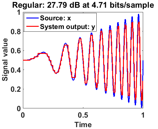
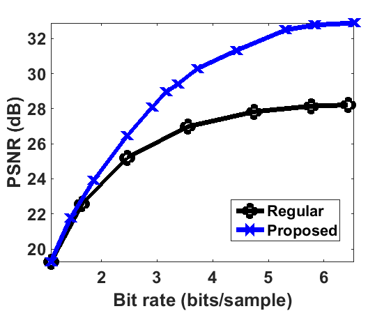
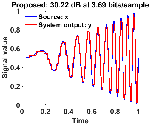
Figure 2: Experiment for one-dimensional signal and adaptive tree-based coding in an acquisition-rendering system. The amplitude-modulated chirp source signal is the blue curve in (a) and (b). The red curves in (a) and (b) are the system output (rendered) signals resulting from regular compression and the proposed method, respectively. (c) Comparison of PSNR-bitrate curves.

III-B Problem Solution in Theory and Practice

While the theoretic framework above considers a cyclo-stationary Gaussian signal and a noiseless system composed of linear shift-invariant operators, the solution presented exhibits important ideas that also appear in the practical method of Section II. Recall that our method is designed for the operational settings of the problem treating non-Gaussian signals and general linear operators, hence, the resemblances between the above theory and practice are at the conceptual level and may materialize differently.

We addressed the theoretic problem (18) using a simple inverse filtering of the input data 𝐰𝐰\mathbf{w}, transforming the problem into (20) and (21) that were solved using an extended version of the standard reverse water-filling procedure. Analogously, our practical method (Algorithm 1) repeatedly compresses a signal formed by an 2subscript2\ell_{2}-constrained deconvolution filtering, that can be rewritten also as a pseudoinverse filtering of the input followed by a weighted averaging with 𝐯~(t)superscript~𝐯𝑡\tilde{\mathbf{v}}^{(t)}, i.e.,

𝐳^(t)=(𝐁𝐀𝐀𝐁+β~𝐈)1(𝐁𝐀𝐀𝐁𝐰~+β~𝐯~(t)).superscript^𝐳𝑡superscriptsuperscript𝐁superscript𝐀𝐀𝐁~𝛽𝐈1superscript𝐁superscript𝐀𝐀𝐁~𝐰~𝛽superscript~𝐯𝑡\displaystyle\hat{\mathbf{z}}^{(t)}=\left(\mathbf{B}^{*}\mathbf{A}^{*}\mathbf{A}\mathbf{B}+\tilde{\beta}\mathbf{I}\right)^{-1}\left(\mathbf{B}^{*}\mathbf{A}^{*}\mathbf{A}\mathbf{B}\tilde{\mathbf{w}}+\tilde{\beta}\tilde{\mathbf{v}}^{(t)}\right).~{}~{}~{} (27)

This shows that, in practice as well as in theory, the input 𝐰𝐰\mathbf{w} should go through a pseudoinverse filtering (softened via (27)) as a preceding stage to compression.

The second prominent principle of the theoretic solution, exhibited in (26), is to compensate for the modulation applied by the pseudoinverse filter corresponding to the effective system operator 𝐀𝐁𝐀𝐁\mathbf{A}\mathbf{B}. Similarly in Algorithm 1, the constrained deconvolution stage (27) implements this idea by better preserving 𝐰~~𝐰\tilde{\mathbf{w}} components corresponding to higher energy parts of 𝐀𝐁𝐀𝐁\mathbf{A}\mathbf{B}. This is clearly observed in the particular case of circulant 𝐀𝐀\mathbf{A} and 𝐁𝐁\mathbf{B}, where the filtering (27) reduces to the DFT-domain component-level operation of

z^kF,(t)=(|akFbkF|2w~kF+β~v~kF,(t))/(|akFbkF|2+β~)subscriptsuperscript^𝑧𝐹𝑡𝑘superscriptsubscriptsuperscript𝑎𝐹𝑘subscriptsuperscript𝑏𝐹𝑘2subscriptsuperscript~𝑤𝐹𝑘~𝛽subscriptsuperscript~𝑣𝐹𝑡𝑘superscriptsubscriptsuperscript𝑎𝐹𝑘subscriptsuperscript𝑏𝐹𝑘2~𝛽\displaystyle\hat{{z}}^{F,(t)}_{k}=\left(\left|a^{F}_{k}b^{F}_{k}\right|^{2}\tilde{{w}}^{F}_{k}+\tilde{\beta}\tilde{{v}}^{F,(t)}_{k}\right)/\left({\left|a^{F}_{k}b^{F}_{k}\right|^{2}+\tilde{\beta}}\right) (28)

where w~kFsubscriptsuperscript~𝑤𝐹𝑘\tilde{{w}}^{F}_{k} and v~kF,(t)subscriptsuperscript~𝑣𝐹𝑡𝑘\tilde{{v}}^{F,(t)}_{k} are the kthsuperscript𝑘𝑡k^{th} DFT-coefficients of 𝐰~~𝐰\tilde{\mathbf{w}} and 𝐯~(t)superscript~𝐯𝑡\tilde{\mathbf{v}}^{(t)}, respectively.

IV Experimental Results

In this section we employ Algorithm 1 to adjust standard compression designs to acquisition-rendering systems where the compression is an intermediate stage. Specifically, we model the source as a high-resolution discrete signal, acquired via linear shift-invariant low-pass filtering and uniform sub-sampling. Then, this acquired signal is available for compression, and after decompression it is linearly rendered back to the source resolution by replicating each decompressed sample (in a uniform pattern matching the source sub-sampling).

IV-1 Coding of One Dimensional Signals

The compression approach here relies on adaptive tree-based segmentation of the signal (for another instance of this prevalent idea see [16]). Specifically, here we compress a one-dimensional signal using an operational rate-distortion optimization determining a binary-tree corresponding to a non-uniform segmentation of the signal, where each segment is represented by a constant value defined by the quantized average-value of the interval (see more details in Appendix D). We consider the system flow of acquisition-compression-decompression-rendering for an amplitude-modulated chirp source signal. Figures 2a and 2b exhibit the system output (i.e., the rendered signal) resulting from the use of a regular compression at 4.71 bpp and from employing our method at 3.69 bpp, respectively. Evidently, our method outperforms the regular approach in terms of PSNR and also in reproducing the chirp signal peaks. Comparing our method to the regular approach at various bit-rates (Fig. 2c) shows significant PSNR gains at medium/high bit-rates.

IV-2 Video Coding

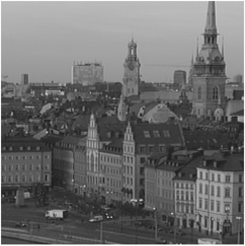
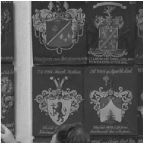
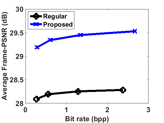
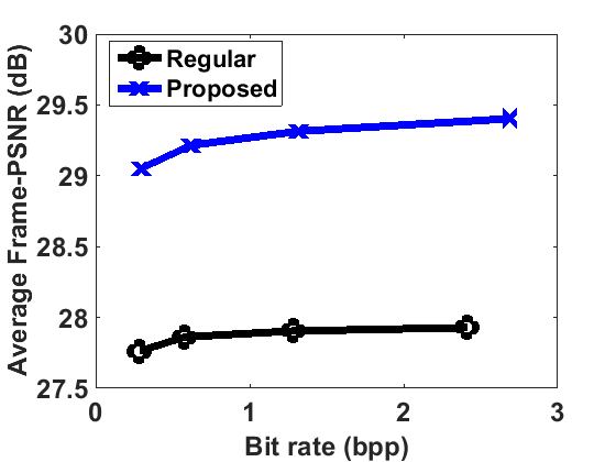
We evaluated our method also for adjusting the HEVC coding standard [13] to a simplified acquisition-rendering system, considering the spatial dimensions of the frames (more details are provided in Appendix E). The PSNR-bitrate curves in Fig. 3 and the visual results (see Appendix E) show the capability of our approach for generically adapting a complicated compression method to a given system structure.
Refer to caption
(a) ’Stockholm’ video
Refer to caption
(b) ’Shields’ video
Figure 3: HEVC coding of 10 video frames. The curves present the PSNR of the system rendered output with respect to the high-resolution source.

V Conclusion

In this paper we considered a system employing lossy compression as an intermediate stage, and proposed a methodology to optimize the system rate-distortion performance from the compression standpoint. We presented a generic operational method and explained its main ideas using rate-distortion theory of Gaussian signals. We provided experimental demonstrations of the effectiveness of our approach for coding of 1D signals and video sequences.

Acknowledgment

This research was supported in part by the European Research Council under European Union’s Seventh Framework Program, ERC Grant agreement no. 320649, and by the Israel Science Foundation grant no. 2597/16.

References

  • [1] S. Boyd, N. Parikh, E. Chu, B. Peleato, and J. Eckstein, “Distributed optimization and statistical learning via the alternating direction method of multipliers,” Foundations and Trends in Machine Learning, vol. 3, no. 1, pp. 1–122, 2011.
  • [2] Y. Dar, M. Elad, and A. M. Bruckstein, “Restoration by compression,” arXiv preprint arXiv:1711.05147, 2017.
  • [3] ——, “Optimized pre-compensating compression,” arXiv preprint arXiv:1711.07901, 2017.
  • [4] M. V. Afonso, J. M. Bioucas-Dias, and M. A. Figueiredo, “Fast image recovery using variable splitting and constrained optimization,” IEEE Trans. Image Process., vol. 19, no. 9, pp. 2345–2356, 2010.
  • [5] S. V. Venkatakrishnan, C. A. Bouman, and B. Wohlberg, “Plug-and-play priors for model based reconstruction,” in IEEE GlobalSIP, 2013.
  • [6] Y. Dar, A. M. Bruckstein, M. Elad, and R. Giryes, “Postprocessing of compressed images via sequential denoising,” IEEE Trans. Image Process., vol. 25, no. 7, pp. 3044–3058, 2016.
  • [7] A. Rond, R. Giryes, and M. Elad, “Poisson inverse problems by the plug-and-play scheme,” Journal of Visual Communication and Image Representation, vol. 41, pp. 96–108, 2016.
  • [8] Y. Romano, M. Elad, and P. Milanfar, “The little engine that could: Regularization by denoising (red),” SIAM Journal on Imaging Sciences, vol. 10, no. 4, pp. 1804–1844, 2017.
  • [9] R. Dobrushin and B. Tsybakov, “Information transmission with additional noise,” IRE Trans. Inf. Theory, vol. 8, no. 5, pp. 293–304, 1962.
  • [10] J. Wolf and J. Ziv, “Transmission of noisy information to a noisy receiver with minimum distortion,” IEEE Trans. Inf. Theory, vol. 16, no. 4, pp. 406–411, 1970.
  • [11] O. K. Al-Shaykh and R. M. Mersereau, “Lossy compression of noisy images,” IEEE Trans. Image Process., vol. 7, no. 12, pp. 1641–1652, 1998.
  • [12] A. Kipnis, A. J. Goldsmith, Y. C. Eldar, and T. Weissman, “Distortion rate function of sub-Nyquist sampled Gaussian sources,” IEEE Trans. Inf. Theory, vol. 62, no. 1, pp. 401–429, 2016.
  • [13] G. J. Sullivan, J. Ohm, W.-J. Han, and T. Wiegand, “Overview of the high efficiency video coding (hevc) standard,” IEEE Trans. Circuits and Systems for Video Technology, vol. 22, no. 12, pp. 1649–1668, 2012.
  • [14] Y. Shoham and A. Gersho, “Efficient bit allocation for an arbitrary set of quantizers,” IEEE Trans. Acoust., Speech, Signal Process., vol. 36, no. 9, pp. 1445–1453, 1988.
  • [15] A. Ortega and K. Ramchandran, “Rate-distortion methods for image and video compression,” IEEE Signal Process. Mag., vol. 15, no. 6, pp. 23–50, 1998.
  • [16] R. Shukla, P. L. Dragotti, M. N. Do, and M. Vetterli, “Rate-distortion optimized tree-structured compression algorithms for piecewise polynomial images,” IEEE Trans. Image Process., vol. 14, no. 3, pp. 343–359, 2005.
  • [17] P. A. Chou, T. Lookabaugh, and R. M. Gray, “Optimal pruning with applications to tree-structured source coding and modeling,” IEEE Trans. Inf. Theory, vol. 35, no. 2, pp. 299–315, 1989.
  • [18] H. Everett III, “Generalized lagrange multiplier method for solving problems of optimum allocation of resources,” Operations research, vol. 11, no. 3, pp. 399–417, 1963.

Appendix A The Theoretic Settings: Minimal Expected Distortion

The minimal distortion was defined in (6) for the operational settings. Here we will formulate its expected value, needed for the statistical settings of Section III. Expecting (6), considering M=N𝑀𝑁M=N and no noise, gives

E{D0}𝐸subscript𝐷0\displaystyle E\left\{D_{0}\right\} =\displaystyle= 1NE{𝐀(𝐈𝐏𝐁)𝐱22}1𝑁𝐸superscriptsubscriptnorm𝐀𝐈subscript𝐏𝐁𝐱22\displaystyle\frac{1}{N}E\left\{\left\|{\mathbf{A}\left(\mathbf{I}-\mathbf{P}_{\mathbf{B}}\right)\mathbf{x}}\right\|_{2}^{2}\right\} (29)
=\displaystyle= 1NE{𝐅𝚲𝐀𝐅𝐅(𝐈𝚲𝐏𝐁)𝐅𝐱22}1𝑁𝐸superscriptsubscriptnormsuperscript𝐅subscript𝚲𝐀superscript𝐅𝐅𝐈subscript𝚲subscript𝐏𝐁𝐅𝐱22\displaystyle\frac{1}{N}E\left\{\left\|{\mathbf{F}^{*}\mathbf{\Lambda}_{\mathbf{A}}\mathbf{F}\mathbf{F}^{*}\left(\mathbf{I}-\mathbf{\Lambda}_{\mathbf{P}_{\mathbf{B}}}\right)\mathbf{F}\mathbf{x}}\right\|_{2}^{2}\right\}
=\displaystyle= 1NE{𝚲𝐀(𝐈𝚲𝐏𝐁)𝐱F22}1𝑁𝐸superscriptsubscriptnormsubscript𝚲𝐀𝐈subscript𝚲subscript𝐏𝐁superscript𝐱𝐹22\displaystyle\frac{1}{N}E\left\{\left\|{\mathbf{\Lambda}_{\mathbf{A}}\left(\mathbf{I}-\mathbf{\Lambda}_{\mathbf{P}_{\mathbf{B}}}\right)\mathbf{x}^{F}}\right\|_{2}^{2}\right\}
=\displaystyle= 1NE{k:akF0,bkF=0|akFxkF|2}1𝑁𝐸subscript:𝑘formulae-sequencesuperscriptsubscript𝑎𝑘𝐹0superscriptsubscript𝑏𝑘𝐹0superscriptsuperscriptsubscript𝑎𝑘𝐹superscriptsubscript𝑥𝑘𝐹2\displaystyle\frac{1}{N}E\left\{\sum\limits_{k:a_{k}^{F}\neq 0~{},~{}b_{k}^{F}=0}\left\lvert{a_{k}^{F}{x}_{k}^{F}}\right\rvert^{2}\right\}
=\displaystyle= 1Nk:akF0,bkF=0|akF|2λk(𝐱),1𝑁subscript:𝑘formulae-sequencesuperscriptsubscript𝑎𝑘𝐹0superscriptsubscript𝑏𝑘𝐹0superscriptsuperscriptsubscript𝑎𝑘𝐹2superscriptsubscript𝜆𝑘𝐱\displaystyle\frac{1}{N}\sum\limits_{k:a_{k}^{F}\neq 0~{},~{}b_{k}^{F}=0}{\left\lvert a_{k}^{F}\right\rvert^{2}\lambda_{k}^{\left(\mathbf{x}\right)}},

where 𝐱F𝐅𝐱superscript𝐱𝐹𝐅𝐱\mathbf{x}^{F}\triangleq\mathbf{F}\mathbf{x}. Furthermore, we used the circulant structure of 𝐏𝐁subscript𝐏𝐁\mathbf{P}_{\mathbf{B}} (as it is the projection matrix corresponding to the range of the circulant matrix 𝐁𝐁\mathbf{B}) providing the DFT-based diagonalization via 𝐅𝐏𝐁𝐅=𝚲𝐏𝐁subscript𝐅𝐏𝐁superscript𝐅subscript𝚲subscript𝐏𝐁\mathbf{F}\mathbf{P}_{\mathbf{B}}\mathbf{F}^{*}=\mathbf{\Lambda}_{\mathbf{P}_{\mathbf{B}}}. Moreover, we utilized the formation of the diagonal matrix 𝚲𝐏𝐁subscript𝚲subscript𝐏𝐁\mathbf{\Lambda}_{\mathbf{P}_{\mathbf{B}}} where the (k,k)𝑘𝑘\left(k,k\right) entry is 1 for k𝑘k corresponding to bkF0superscriptsubscript𝑏𝑘𝐹0b_{k}^{F}\neq 0, and otherwise the (k,k)𝑘𝑘\left(k,k\right) entry is 0.

Appendix B The Theoretic Settings: Equivalence of Optimization Problems (18) and (20)

Let us begin by proving the equivalence between the distortion constraints of optimizations (18) and (20). We define the matrix 𝐇𝐀𝐁𝐇𝐀𝐁\mathbf{H}\triangleq\mathbf{A}\mathbf{B} joining the two linear operators of the system. In Section III we considered 𝐀𝐀\mathbf{A} and 𝐁𝐁\mathbf{B} to be N×N𝑁𝑁N\times N circulant matrices and, thus, 𝐇𝐇\mathbf{H} is also a N×N𝑁𝑁N\times N circulant matrix. Consequently, 𝐇𝐇\mathbf{H} is diagonalized by the N×N𝑁𝑁N\times N DFT matrix 𝐅𝐅\mathbf{F} via 𝐅𝐇𝐅=𝚲𝐇superscript𝐅𝐇𝐅subscript𝚲𝐇\mathbf{F}\mathbf{H}\mathbf{F}^{*}=\mathbf{\Lambda}_{\mathbf{H}}, where 𝚲𝐇subscript𝚲𝐇\mathbf{\Lambda}_{\mathbf{H}} is a diagonal matrix formed by the elements hkF=akFbkFsubscriptsuperscript𝐹𝑘subscriptsuperscript𝑎𝐹𝑘subscriptsuperscript𝑏𝐹𝑘h^{F}_{k}=a^{F}_{k}b^{F}_{k} for k=0,,N1𝑘0𝑁1k=0,...,N-1. The pseudoinverse matrix of 𝐇𝐇\mathbf{H} is defined as 𝐇+=𝐅𝚲𝐇+𝐅superscript𝐇superscript𝐅superscriptsubscript𝚲𝐇𝐅\mathbf{H}^{+}=\mathbf{F}^{*}\mathbf{\Lambda}_{\mathbf{H}}^{+}\mathbf{F}, where 𝚲𝐇+superscriptsubscript𝚲𝐇\mathbf{\Lambda}_{\mathbf{H}}^{+} is the pseudoinverse of 𝚲𝐇subscript𝚲𝐇\mathbf{\Lambda}_{\mathbf{H}}, an N×N𝑁𝑁N\times N diagonal matrix with the kthsuperscript𝑘𝑡k^{th} diagonal component

hkF,+={1akFbkF,for k𝒦AB0,for k𝒦AB.\displaystyle h^{F,+}_{k}=\left\{{\begin{array}[]{*{20}{c}}{\frac{1}{a^{F}_{k}b^{F}_{k}}}&{,\text{for~{}~{}}k\in\mathcal{K}_{AB}}\\ 0&{,\text{for~{}~{}}k\notin\mathcal{K}_{AB}.}\end{array}}\right. (32)

where 𝒦AB{k:akF0andbkF0}subscript𝒦𝐴𝐵conditional-set𝑘superscriptsubscript𝑎𝑘𝐹0andsuperscriptsubscript𝑏𝑘𝐹0\mathcal{K}_{AB}\nolinebreak\triangleq\nolinebreak\left\{k:a_{k}^{F}\neq 0~{}\text{and}~{}b_{k}^{F}\neq 0\right\} includes the DFT-domain component indices defining the range of the joint operator 𝐀𝐁𝐀𝐁\mathbf{AB}.

Now, let us develop the distortion expression appearing in the constraint of optimization (18):

𝐰𝐀𝐁𝐯22superscriptsubscriptnorm𝐰𝐀𝐁𝐯22\displaystyle\left\|{\mathbf{w}-\mathbf{A}\mathbf{B}\mathbf{v}}\right\|_{2}^{2} =\displaystyle= 𝐰𝐇𝐯22superscriptsubscriptnorm𝐰𝐇𝐯22\displaystyle\left\|{\mathbf{w}-\mathbf{H}\mathbf{v}}\right\|_{2}^{2}
=\displaystyle= (𝐈𝐇𝐇+)𝐰+𝐇𝐇+𝐰𝐇𝐯22superscriptsubscriptnorm𝐈superscript𝐇𝐇𝐰superscript𝐇𝐇𝐰𝐇𝐯22\displaystyle\left\|{\left(\mathbf{I}-\mathbf{H}\mathbf{H}^{+}\right)\mathbf{w}+\mathbf{H}\mathbf{H}^{+}\mathbf{w}-\mathbf{H}\mathbf{v}}\right\|_{2}^{2}
=\displaystyle= (𝐈𝐇𝐇+)𝐰+𝐇(𝐇+𝐰𝐯)22superscriptsubscriptnorm𝐈superscript𝐇𝐇𝐰𝐇superscript𝐇𝐰𝐯22\displaystyle\left\|{\left(\mathbf{I}-\mathbf{H}\mathbf{H}^{+}\right)\mathbf{w}+\mathbf{H}\left(\mathbf{H}^{+}\mathbf{w}-\mathbf{v}\right)}\right\|_{2}^{2}
=\displaystyle= (𝐈𝐇𝐇+)𝐰22+𝐇(𝐇+𝐰𝐯)22superscriptsubscriptnorm𝐈superscript𝐇𝐇𝐰22superscriptsubscriptnorm𝐇superscript𝐇𝐰𝐯22\displaystyle\left\|{\left(\mathbf{I}-\mathbf{H}\mathbf{H}^{+}\right)\mathbf{w}}\right\|_{2}^{2}+\left\|{\mathbf{H}\left(\mathbf{H}^{+}\mathbf{w}-\mathbf{v}\right)}\right\|_{2}^{2}
+(𝐇+𝐰𝐯)𝐇(𝐈𝐇𝐇+)𝐰superscriptsuperscript𝐇𝐰𝐯superscript𝐇𝐈superscript𝐇𝐇𝐰\displaystyle+\left(\mathbf{H}^{+}\mathbf{w}-\mathbf{v}\right)^{*}\mathbf{H}^{*}\left(\mathbf{I}-\mathbf{H}\mathbf{H}^{+}\right)\mathbf{w}
+𝐰(𝐈𝐇𝐇+)𝐇(𝐇+𝐰𝐯)superscript𝐰superscript𝐈superscript𝐇𝐇𝐇superscript𝐇𝐰𝐯\displaystyle+\mathbf{w}^{*}\left(\mathbf{I}-\mathbf{H}\mathbf{H}^{+}\right)^{*}\mathbf{H}\left(\mathbf{H}^{+}\mathbf{w}-\mathbf{v}\right)
=\displaystyle= (𝐈𝐇𝐇+)𝐰22+𝐇(𝐇+𝐰𝐯)22superscriptsubscriptnorm𝐈superscript𝐇𝐇𝐰22superscriptsubscriptnorm𝐇superscript𝐇𝐰𝐯22\displaystyle\left\|{\left(\mathbf{I}-\mathbf{H}\mathbf{H}^{+}\right)\mathbf{w}}\right\|_{2}^{2}+\left\|{\mathbf{H}\left(\mathbf{H}^{+}\mathbf{w}-\mathbf{v}\right)}\right\|_{2}^{2}~{}~{}~{}~{}

where the last equality readily stems from the relation

𝐇(𝐈𝐇𝐇+)=𝟎.superscript𝐇𝐈superscript𝐇𝐇0\displaystyle\mathbf{H}^{*}\left(\mathbf{I}-\mathbf{H}\mathbf{H}^{+}\right)=\mathbf{0}. (34)

We use the DFT-based diagonalization of 𝐇𝐇\mathbf{H} to continue developing the expression of the first term in (B):

(𝐈𝐇𝐇+)𝐰22superscriptsubscriptnorm𝐈superscript𝐇𝐇𝐰22\displaystyle\left\|{\left(\mathbf{I}-\mathbf{H}\mathbf{H}^{+}\right)\mathbf{w}}\right\|_{2}^{2} =\displaystyle= (𝐈𝐅𝚲𝐇𝐅𝐅𝚲𝐇+𝐅)𝐰22superscriptsubscriptnorm𝐈superscript𝐅subscript𝚲𝐇superscript𝐅𝐅superscriptsubscript𝚲𝐇𝐅𝐰22\displaystyle\left\|{\left(\mathbf{I}-\mathbf{F}^{*}\mathbf{\Lambda}_{\mathbf{H}}\mathbf{F}\mathbf{F}^{*}\mathbf{\Lambda}_{\mathbf{H}}^{+}\mathbf{F}\right)\mathbf{w}}\right\|_{2}^{2} (35)
=\displaystyle= 𝐅(𝐈𝚲𝐇𝚲𝐇+)𝐅𝐰22superscriptsubscriptnormsuperscript𝐅𝐈subscript𝚲𝐇superscriptsubscript𝚲𝐇𝐅𝐰22\displaystyle\left\|{\mathbf{F}^{*}\left(\mathbf{I}-\mathbf{\Lambda}_{\mathbf{H}}\mathbf{\Lambda}_{\mathbf{H}}^{+}\right)\mathbf{F}\mathbf{w}}\right\|_{2}^{2}
=\displaystyle= (𝐈𝚲𝐇𝚲𝐇+)𝐰F22superscriptsubscriptnorm𝐈subscript𝚲𝐇superscriptsubscript𝚲𝐇superscript𝐰𝐹22\displaystyle\left\|{\left(\mathbf{I}-\mathbf{\Lambda}_{\mathbf{H}}\mathbf{\Lambda}_{\mathbf{H}}^{+}\right)\mathbf{w}^{F}}\right\|_{2}^{2}
=\displaystyle= k:hkF=0|wkF|2=subscript:𝑘superscriptsubscript𝑘𝐹0superscriptsuperscriptsubscript𝑤𝑘𝐹2absent\displaystyle\sum\limits_{k:h_{k}^{F}=0}\left\lvert w_{k}^{F}\right\rvert^{2}=
=\displaystyle= k:akF0,bkF=0|akFxkF|2subscript:𝑘formulae-sequencesuperscriptsubscript𝑎𝑘𝐹0superscriptsubscript𝑏𝑘𝐹0superscriptsuperscriptsubscript𝑎𝑘𝐹superscriptsubscript𝑥𝑘𝐹2\displaystyle\sum\limits_{k:a_{k}^{F}\neq 0,b_{k}^{F}=0}\left\lvert a_{k}^{F}x_{k}^{F}\right\rvert^{2}

where we used the DFT-domain expression of the kthsuperscript𝑘𝑡k^{th} component of 𝐰Fsuperscript𝐰𝐹\mathbf{w}^{F} as wkF=akFxkFsuperscriptsubscript𝑤𝑘𝐹superscriptsubscript𝑎𝑘𝐹superscriptsubscript𝑥𝑘𝐹w_{k}^{F}=a_{k}^{F}x_{k}^{F}, reducing to wkF=0superscriptsubscript𝑤𝑘𝐹0w_{k}^{F}=0 when akF=0superscriptsubscript𝑎𝑘𝐹0a_{k}^{F}=0. Taking the expectation of (35), noting that the source signal 𝐱𝐱\mathbf{x} and the noise 𝐧𝐧\mathbf{n} are independent, yields

E{(𝐈𝐇𝐇+)𝐰22}=k:akF0,bkF=0|akF|2λk(𝐱).𝐸superscriptsubscriptnorm𝐈superscript𝐇𝐇𝐰22subscript:𝑘formulae-sequencesuperscriptsubscript𝑎𝑘𝐹0superscriptsubscript𝑏𝑘𝐹0superscriptsuperscriptsubscript𝑎𝑘𝐹2superscriptsubscript𝜆𝑘𝐱\displaystyle E\left\{\left\|{\left(\mathbf{I}-\mathbf{H}\mathbf{H}^{+}\right)\mathbf{w}}\right\|_{2}^{2}\right\}=\sum\limits_{k:a_{k}^{F}\neq 0~{},~{}b_{k}^{F}=0}{\left\lvert a_{k}^{F}\right\rvert^{2}\lambda_{k}^{\left(\mathbf{x}\right)}}. (36)

Then, using (B) and (36) we get that

E{𝐰𝐀𝐁𝐯22}𝐸superscriptsubscriptnorm𝐰𝐀𝐁𝐯22\displaystyle E\left\{\left\|{\mathbf{w}-\mathbf{A}\mathbf{B}\mathbf{v}}\right\|_{2}^{2}\right\} =\displaystyle= E{𝐀𝐁(𝐰~𝐯)22}𝐸superscriptsubscriptnorm𝐀𝐁~𝐰𝐯22\displaystyle E\left\{\left\|{\mathbf{A}\mathbf{B}\left(\tilde{\mathbf{w}}-\mathbf{v}\right)}\right\|_{2}^{2}\right\}
+k:akF0,bkF=0|akF|2λk(𝐱),subscript:𝑘formulae-sequencesuperscriptsubscript𝑎𝑘𝐹0superscriptsubscript𝑏𝑘𝐹0superscriptsuperscriptsubscript𝑎𝑘𝐹2superscriptsubscript𝜆𝑘𝐱\displaystyle+\sum\limits_{k:a_{k}^{F}\neq 0~{},~{}b_{k}^{F}=0}{\left\lvert a_{k}^{F}\right\rvert^{2}\lambda_{k}^{\left(\mathbf{x}\right)}},

where 𝐰~=𝐁+𝐀+𝐰~𝐰superscript𝐁superscript𝐀𝐰\tilde{\mathbf{w}}=\mathbf{B}^{+}\mathbf{A}^{+}\mathbf{w}. Eq. (29) implies

NE{D0}=k:akF0,bkF=0|akF|2λk(𝐱)𝑁𝐸subscript𝐷0subscript:𝑘formulae-sequencesuperscriptsubscript𝑎𝑘𝐹0superscriptsubscript𝑏𝑘𝐹0superscriptsuperscriptsubscript𝑎𝑘𝐹2superscriptsubscript𝜆𝑘𝐱\displaystyle NE\left\{D_{0}\right\}=\sum\limits_{k:a_{k}^{F}\neq 0~{},~{}b_{k}^{F}=0}{\left\lvert a_{k}^{F}\right\rvert^{2}\lambda_{k}^{\left(\mathbf{x}\right)}} (38)

that jointly with (B) yields the transformation of the expected distortion constraint in the optimization (18), namely,

NE{D0}E{𝐰𝐀𝐁𝐯22}N(E{D0}+D)𝑁𝐸subscript𝐷0𝐸superscriptsubscriptnorm𝐰𝐀𝐁𝐯22𝑁𝐸subscript𝐷0𝐷\displaystyle NE\left\{D_{0}\right\}\leq E\left\{\left\|{\mathbf{w}-\mathbf{A}\mathbf{B}\mathbf{v}}\right\|_{2}^{2}\right\}\leq N\left(E\left\{D_{0}\right\}+D\right)~{}~{} (39)

into

0E{𝐀𝐁(𝐰~𝐯)22}ND.0𝐸superscriptsubscriptnorm𝐀𝐁~𝐰𝐯22𝑁𝐷\displaystyle 0\leq E\left\{\left\|{\mathbf{A}\mathbf{B}\left(\tilde{\mathbf{w}}-\mathbf{v}\right)}\right\|_{2}^{2}\right\}\leq ND. (40)

Since (40) is the distortion constraint in optimization (20), we proved that the distortion constraints of optimizations (18) and (20) are interchangeable.

We continue by showing the equivalence of the mutual information terms appearing in the optimization costs of (18) and (20). We start with I(𝐰;𝐁𝐯)𝐼𝐰𝐁𝐯I\left(\mathbf{w};\mathbf{B}\mathbf{v}\right) used in (18). By the data processing inequality, the compression-input 𝐰𝐰\mathbf{w} and its filtered version 𝐀+𝐰superscript𝐀𝐰\mathbf{A}^{+}{\mathbf{w}} obey

I(𝐰;𝐁𝐯)I(𝐀+𝐰;𝐁𝐯).𝐼𝐰𝐁𝐯𝐼superscript𝐀𝐰𝐁𝐯\displaystyle I\left(\mathbf{w};\mathbf{B}\mathbf{v}\right)\geq I\left(\mathbf{A}^{+}{\mathbf{w}};\mathbf{B}\mathbf{v}\right). (41)

In the theoretic settings we consider the noiseless case where 𝐰=𝐀𝐱𝐰𝐀𝐱\mathbf{w}=\mathbf{A}\mathbf{x}, hence, 𝐀+𝐰=𝐏𝐀𝐱superscript𝐀𝐰subscript𝐏𝐀𝐱\mathbf{A}^{+}{\mathbf{w}}=\mathbf{P}_{\mathbf{A}}\mathbf{x}. Recall that 𝐏𝐀subscript𝐏𝐀\mathbf{P}_{\mathbf{A}} is the projection matrix of the range of 𝐀𝐀\mathbf{A}. Since 𝐀𝐀\mathbf{A} is circulant, 𝐏𝐀subscript𝐏𝐀\mathbf{P}_{\mathbf{A}} is also circulant and diagonalized by the DFT matrix via 𝐅𝐏𝐀𝐅=𝚲𝐏𝐀subscript𝐅𝐏𝐀superscript𝐅subscript𝚲subscript𝐏𝐀\mathbf{F}\mathbf{P}_{\mathbf{A}}\mathbf{F}^{*}=\mathbf{\Lambda}_{\mathbf{P}_{\mathbf{A}}} where 𝚲𝐏𝐀=𝚲𝐀𝚲𝐀+subscript𝚲subscript𝐏𝐀subscript𝚲𝐀superscriptsubscript𝚲𝐀\mathbf{\Lambda}_{\mathbf{P}_{\mathbf{A}}}=\mathbf{\Lambda}_{{\mathbf{A}}}\mathbf{\Lambda}_{{\mathbf{A}}}^{+}. Accordingly, we can write

𝐀𝐀+𝐰=𝐀𝐏𝐀𝐱=𝐀𝐱=𝐰superscript𝐀𝐀𝐰subscript𝐀𝐏𝐀𝐱𝐀𝐱𝐰\displaystyle\mathbf{A}\mathbf{A}^{+}{\mathbf{w}}=\mathbf{A}\mathbf{P}_{\mathbf{A}}\mathbf{x}=\mathbf{A}\mathbf{x}=\mathbf{w} (42)

exhibiting 𝐰𝐰\mathbf{w} as a processing of 𝐀+𝐰superscript𝐀𝐰\mathbf{A}^{+}{\mathbf{w}}, thus, by the data processing inequality we get

I(𝐰;𝐁𝐯)I(𝐀+𝐰;𝐁𝐯)𝐼𝐰𝐁𝐯𝐼superscript𝐀𝐰𝐁𝐯\displaystyle I\left(\mathbf{w};\mathbf{B}\mathbf{v}\right)\leq I\left(\mathbf{A}^{+}{\mathbf{w}};\mathbf{B}\mathbf{v}\right) (43)

that together with (41) implies

I(𝐰;𝐁𝐯)=I(𝐀+𝐰;𝐁𝐯).𝐼𝐰𝐁𝐯𝐼superscript𝐀𝐰𝐁𝐯\displaystyle I\left(\mathbf{w};\mathbf{B}\mathbf{v}\right)=I\left(\mathbf{A}^{+}{\mathbf{w}};\mathbf{B}\mathbf{v}\right). (44)

The above showed that since 𝐰𝐰\mathbf{w} is in the range of 𝐀𝐀\mathbf{A}, its processing via 𝐀+superscript𝐀\mathbf{A}^{+} is invertible and, thus, the mutual information is preserved under such processing of 𝐰𝐰\mathbf{w}.

Similar to the above arguments, we can show that since the system output 𝐁𝐯𝐁𝐯\mathbf{B}\mathbf{v} is in the range of 𝐁𝐁\mathbf{B}, its processing via 𝐁+superscript𝐁\mathbf{B}^{+} is invertible and, therefore, the mutual information is preserved under such filtering of 𝐁𝐯𝐁𝐯\mathbf{B}\mathbf{v}:

I(𝐀+𝐰;𝐁𝐯)𝐼superscript𝐀𝐰𝐁𝐯\displaystyle I\left(\mathbf{A}^{+}{\mathbf{w}};\mathbf{B}\mathbf{v}\right) =\displaystyle= I(𝐀+𝐰;𝐁+𝐁𝐯)𝐼superscript𝐀𝐰superscript𝐁𝐁𝐯\displaystyle I\left(\mathbf{A}^{+}{\mathbf{w}};\mathbf{B}^{+}\mathbf{B}\mathbf{v}\right) (45)
=\displaystyle= I(𝐀+𝐰;𝐏𝐁𝐯).𝐼superscript𝐀𝐰subscript𝐏𝐁𝐯\displaystyle I\left(\mathbf{A}^{+}{\mathbf{w}};\mathbf{P}_{\mathbf{B}}\mathbf{v}\right).

Consider the decomposition of 𝐀+𝐰superscript𝐀𝐰\mathbf{A}^{+}{\mathbf{w}} based on its projections on 𝐁𝐁\mathbf{B}’s range and nullspace, namely,

𝐀+𝐰=𝐏𝐁𝐀+𝐰+(𝐈𝐏𝐁)𝐀+𝐰.superscript𝐀𝐰subscript𝐏𝐁superscript𝐀𝐰𝐈subscript𝐏𝐁superscript𝐀𝐰\displaystyle\mathbf{A}^{+}{\mathbf{w}}=\mathbf{P}_{\mathbf{B}}\mathbf{A}^{+}{\mathbf{w}}+\left(\mathbf{I}-\mathbf{P}_{\mathbf{B}}\right)\mathbf{A}^{+}{\mathbf{w}}. (46)

Observe that

(𝐈𝐏𝐁)𝐀+𝐰𝐈subscript𝐏𝐁superscript𝐀𝐰\displaystyle\left(\mathbf{I}-\mathbf{P}_{\mathbf{B}}\right)\mathbf{A}^{+}{\mathbf{w}} =\displaystyle= 𝐅(𝐈𝚲𝐏𝐁)𝐅𝐅𝚲𝐀+𝐅𝐰superscript𝐅𝐈subscript𝚲subscript𝐏𝐁superscript𝐅𝐅superscriptsubscript𝚲𝐀𝐅𝐰\displaystyle\mathbf{F}^{*}\left(\mathbf{I}-\mathbf{\Lambda}_{\mathbf{P}_{\mathbf{B}}}\right)\mathbf{F}\mathbf{F}^{*}\mathbf{\Lambda}_{\mathbf{A}}^{+}\mathbf{F}{\mathbf{w}} (47)
=\displaystyle= 𝐅(𝐈𝚲𝐏𝐁)𝚲𝐀+𝐰Fsuperscript𝐅𝐈subscript𝚲subscript𝐏𝐁superscriptsubscript𝚲𝐀superscript𝐰𝐹\displaystyle\mathbf{F}^{*}\left(\mathbf{I}-\mathbf{\Lambda}_{\mathbf{P}_{\mathbf{B}}}\right)\mathbf{\Lambda}_{\mathbf{A}}^{+}{\mathbf{w}^{F}}

and the second random variable considered by the mutual information in (45) is

𝐏𝐁𝐯subscript𝐏𝐁𝐯\displaystyle\mathbf{P}_{\mathbf{B}}\mathbf{v} =\displaystyle= 𝐅𝚲𝐏𝐁𝐅𝐰superscript𝐅subscript𝚲subscript𝐏𝐁𝐅𝐰\displaystyle\mathbf{F}^{*}\mathbf{\Lambda}_{\mathbf{P}_{\mathbf{B}}}\mathbf{F}{\mathbf{w}} (48)
=\displaystyle= 𝐅𝚲𝐏𝐁𝐰Fsuperscript𝐅subscript𝚲subscript𝐏𝐁superscript𝐰𝐹\displaystyle\mathbf{F}^{*}\mathbf{\Lambda}_{\mathbf{P}_{\mathbf{B}}}{\mathbf{w}}^{F}

where 𝐰Fsuperscript𝐰𝐹{\mathbf{w}}^{F} is the DFT-domain representation of 𝐰𝐰{\mathbf{w}}. Note that the diagonal projection matrices 𝚲𝐏𝐁𝚲𝐁𝚲𝐁+subscript𝚲subscript𝐏𝐁subscript𝚲𝐁superscriptsubscript𝚲𝐁\mathbf{\Lambda}_{\mathbf{P}_{\mathbf{B}}}\triangleq\mathbf{\Lambda}_{\mathbf{B}}\mathbf{\Lambda}_{\mathbf{B}}^{+} and 𝐈𝚲𝐏𝐁𝐈subscript𝚲subscript𝐏𝐁\mathbf{I}-\mathbf{\Lambda}_{\mathbf{P}_{\mathbf{B}}} appearing in (48) and (47), respectively, imply that the DFT-domain representations of (𝐈𝐏𝐁)𝐀+𝐰𝐈subscript𝐏𝐁superscript𝐀𝐰\left(\mathbf{I}-\mathbf{P}_{\mathbf{B}}\right)\mathbf{A}^{+}{\mathbf{w}} and 𝐏𝐁𝐯subscript𝐏𝐁𝐯\mathbf{P}_{\mathbf{B}}\mathbf{v} have complementary non-overlapping supports (defined by the component indices where the value may be nonzero). Let us develop the mutual information in (45) to leverage the mentioned structures and the decomposition (46):

I(𝐀+𝐰;𝐏𝐁𝐯)=𝐼superscript𝐀𝐰subscript𝐏𝐁𝐯absent\displaystyle I\left(\mathbf{A}^{+}{\mathbf{w}};\mathbf{P}_{\mathbf{B}}\mathbf{v}\right)=
=I(𝐅𝐀+𝐰;𝐅𝐏𝐁𝐯)absent𝐼superscript𝐅𝐀𝐰subscript𝐅𝐏𝐁𝐯\displaystyle=I\left(\mathbf{F}\mathbf{A}^{+}{\mathbf{w}};\mathbf{F}\mathbf{P}_{\mathbf{B}}\mathbf{v}\right) (49)
=I(𝚲𝐀+𝐰F;𝚲𝐏𝐁𝐯F)absent𝐼superscriptsubscript𝚲𝐀superscript𝐰𝐹subscript𝚲subscript𝐏𝐁superscript𝐯𝐹\displaystyle=I\left(\mathbf{\Lambda}_{\mathbf{A}}^{+}{\mathbf{w}^{F}};\mathbf{\Lambda}_{\mathbf{P}_{\mathbf{B}}}\mathbf{v}^{F}\right) (50)
k:bkF0I(akF,+wkF;vkF)+k:bkF=0I(akF,+wkF;0)absentsubscript:𝑘superscriptsubscript𝑏𝑘𝐹0𝐼superscriptsubscript𝑎𝑘𝐹superscriptsubscript𝑤𝑘𝐹superscriptsubscript𝑣𝑘𝐹subscript:𝑘superscriptsubscript𝑏𝑘𝐹0𝐼superscriptsubscript𝑎𝑘𝐹superscriptsubscript𝑤𝑘𝐹0\displaystyle\geq\sum\limits_{k:b_{k}^{F}\neq 0}{I\left(a_{k}^{F,+}{{w}_{k}^{F}};{v}_{k}^{F}\right)}+\sum\limits_{k:b_{k}^{F}=0}{I\left(a_{k}^{F,+}{{w}_{k}^{F}};0\right)} (51)
=k:bkF0I(akF,+wkF;vkF)absentsubscript:𝑘superscriptsubscript𝑏𝑘𝐹0𝐼superscriptsubscript𝑎𝑘𝐹superscriptsubscript𝑤𝑘𝐹superscriptsubscript𝑣𝑘𝐹\displaystyle=\sum\limits_{k:b_{k}^{F}\neq 0}{I\left(a_{k}^{F,+}{{w}_{k}^{F}};{v}_{k}^{F}\right)} (52)

where (49) is due to the preservation of mutual information under a unitary transformation. The lower bound in (51) emerges from the independence of the DFT-domain variables wkFsuperscriptsubscript𝑤𝑘𝐹{{w}_{k}^{F}}, k=0,,N1𝑘0𝑁1k=0,...,N-1, since they originate in the cyclo-stationary Gaussian signal 𝐱𝐱\mathbf{x} processed by the circulant matrix 𝐀𝐀\mathbf{A}. In Appendix C we exhibit a backward channel construction based on independent components vkFsuperscriptsubscript𝑣𝑘𝐹{v}_{k}^{F} in the DFT domain, therefore, satisfying the inequality (51) with equality. Using (52) and pending on the construction shown in Appendix C, we state that

I(𝐀+𝐰;𝐏𝐁𝐯)𝐼superscript𝐀𝐰subscript𝐏𝐁𝐯\displaystyle I\left(\mathbf{A}^{+}{\mathbf{w}};\mathbf{P}_{\mathbf{B}}\mathbf{v}\right) =\displaystyle= k:bkF0I(akF,+wkF;vkF)subscript:𝑘superscriptsubscript𝑏𝑘𝐹0𝐼superscriptsubscript𝑎𝑘𝐹superscriptsubscript𝑤𝑘𝐹superscriptsubscript𝑣𝑘𝐹\displaystyle\sum\limits_{k:b_{k}^{F}\neq 0}{I\left(a_{k}^{F,+}{{w}_{k}^{F}};{v}_{k}^{F}\right)} (53)
=\displaystyle= I(𝐏𝐁𝐀+𝐰;𝐏𝐁𝐯)𝐼subscript𝐏𝐁superscript𝐀𝐰subscript𝐏𝐁𝐯\displaystyle I\left(\mathbf{P}_{\mathbf{B}}\mathbf{A}^{+}{\mathbf{w}};\mathbf{P}_{\mathbf{B}}\mathbf{v}\right)

Note that 𝐏𝐁𝐀+𝐰subscript𝐏𝐁superscript𝐀𝐰\mathbf{P}_{\mathbf{B}}\mathbf{A}^{+}{\mathbf{w}} is in the range of 𝐀𝐀\mathbf{A}, hence, using similar arguments to those given in the last paragraph, one can show that

I(𝐏𝐁𝐀+𝐰;𝐏𝐁𝐯)=I(𝐏𝐁𝐀+𝐰;𝐏𝐀𝐏𝐁𝐯)𝐼subscript𝐏𝐁superscript𝐀𝐰subscript𝐏𝐁𝐯𝐼subscript𝐏𝐁superscript𝐀𝐰subscript𝐏𝐀subscript𝐏𝐁𝐯\displaystyle I\left(\mathbf{P}_{\mathbf{B}}\mathbf{A}^{+}{\mathbf{w}};\mathbf{P}_{\mathbf{B}}\mathbf{v}\right)=I\left(\mathbf{P}_{\mathbf{B}}\mathbf{A}^{+}{\mathbf{w}};\mathbf{P}_{\mathbf{A}}\mathbf{P}_{\mathbf{B}}\mathbf{v}\right) (54)

Furthermore, since 𝐏𝐁𝐀+𝐰subscript𝐏𝐁superscript𝐀𝐰\mathbf{P}_{\mathbf{B}}\mathbf{A}^{+}{\mathbf{w}} belongs also to the range of 𝐁𝐁\mathbf{B}, its processing via 𝐁+superscript𝐁\mathbf{B}^{+} is invertible, thus,

I(𝐏𝐁𝐀+𝐰;𝐏𝐀𝐏𝐁𝐯)=I(𝐁+𝐀+𝐰;𝐏𝐀𝐏𝐁𝐯).𝐼subscript𝐏𝐁superscript𝐀𝐰subscript𝐏𝐀subscript𝐏𝐁𝐯𝐼superscript𝐁superscript𝐀𝐰subscript𝐏𝐀subscript𝐏𝐁𝐯\displaystyle I\left(\mathbf{P}_{\mathbf{B}}\mathbf{A}^{+}{\mathbf{w}};\mathbf{P}_{\mathbf{A}}\mathbf{P}_{\mathbf{B}}\mathbf{v}\right)=I\left(\mathbf{B}^{+}\mathbf{A}^{+}{\mathbf{w}};\mathbf{P}_{\mathbf{A}}\mathbf{P}_{\mathbf{B}}\mathbf{v}\right). (55)

Due to the circulant structure of 𝐏𝐀subscript𝐏𝐀\mathbf{P}_{\mathbf{A}} and 𝐏𝐁subscript𝐏𝐁\mathbf{P}_{\mathbf{B}}, they commute and, therefore,

I(𝐏𝐁𝐀+𝐰;𝐏𝐀𝐏𝐁𝐯)=I(𝐁+𝐀+𝐰;𝐏𝐁𝐏𝐀𝐯),𝐼subscript𝐏𝐁superscript𝐀𝐰subscript𝐏𝐀subscript𝐏𝐁𝐯𝐼superscript𝐁superscript𝐀𝐰subscript𝐏𝐁subscript𝐏𝐀𝐯\displaystyle I\left(\mathbf{P}_{\mathbf{B}}\mathbf{A}^{+}{\mathbf{w}};\mathbf{P}_{\mathbf{A}}\mathbf{P}_{\mathbf{B}}\mathbf{v}\right)=I\left(\mathbf{B}^{+}\mathbf{A}^{+}{\mathbf{w}};\mathbf{P}_{\mathbf{B}}\mathbf{P}_{\mathbf{A}}\mathbf{v}\right), (56)

that is the mutual information in the cost of problem (20). To conclude, we showed the equivalence of the costs (based on the backward-channel construction presented next in Appendix C) and the constraints of problems (18) and (20), therefore, these optimization problems are interchangeable.

Appendix C The Theoretic Settings: Equivalence of Optimization Problems (20) and (21)

Since 𝐀𝐀\mathbf{A} and 𝐁𝐁\mathbf{B} are circulant matrices, the expected distortion E{𝐀𝐁(𝐰~𝐯)22}𝐸superscriptsubscriptnorm𝐀𝐁~𝐰𝐯22E\left\{\left\|{\mathbf{A}\mathbf{B}\left(\tilde{\mathbf{w}}-\mathbf{v}\right)}\right\|_{2}^{2}\right\}, appearing in the constraint of (20), has the following additively-separable form in the DFT domain

E{𝐀𝐁(𝐰~𝐯)22}𝐸superscriptsubscriptnorm𝐀𝐁~𝐰𝐯22\displaystyle E\left\{\left\|{\mathbf{A}\mathbf{B}\left(\tilde{\mathbf{w}}-\mathbf{v}\right)}\right\|_{2}^{2}\right\} =\displaystyle= E{𝚲𝐀𝚲𝐁(𝐰~F𝐯F)22}𝐸superscriptsubscriptnormsubscript𝚲𝐀subscript𝚲𝐁superscript~𝐰𝐹superscript𝐯𝐹22\displaystyle E\left\{\left\|{\mathbf{\Lambda}_{\mathbf{A}}\mathbf{\Lambda}_{\mathbf{B}}\left(\tilde{\mathbf{w}}^{F}-\mathbf{v}^{F}\right)}\right\|_{2}^{2}\right\}~{}~{}~{}~{}~{}~{} (57)
=\displaystyle= k=0N1|akFbkF|2E{|w~kFvkF|2}.superscriptsubscript𝑘0𝑁1superscriptsubscriptsuperscript𝑎𝐹𝑘subscriptsuperscript𝑏𝐹𝑘2𝐸superscriptsubscriptsuperscript~𝑤𝐹𝑘subscriptsuperscript𝑣𝐹𝑘2\displaystyle\sum\limits_{k=0}^{N-1}{\left|a^{F}_{k}b^{F}_{k}\right|^{2}E\left\{\left|{\tilde{w}^{F}_{k}-v^{F}_{k}}\right|^{2}\right\}}.~{}~{}~{}~{}~{}~{}

This expected distortion formulation motivates us to address the entire rate-distortion optimization in the DFT domain and with respect to a pseudoinverse filtered version of the input 𝐰𝐰\mathbf{w}. For this purpose we will treat next the optimization cost of the problem given in (20).

Since 𝐰~𝐁+𝐀+𝐰~𝐰superscript𝐁superscript𝐀𝐰\tilde{\mathbf{w}}\triangleq\mathbf{B}^{+}\mathbf{A}^{+}{\mathbf{w}} is a cyclo-stationary Gaussian signal, we apply the following familiar lower bounds:

I(𝐰~;𝐏𝐁𝐏𝐀𝐯)𝐼~𝐰subscript𝐏𝐁subscript𝐏𝐀𝐯\displaystyle I\left(\tilde{\mathbf{w}};\mathbf{P}_{\mathbf{B}}\mathbf{P}_{\mathbf{A}}\mathbf{v}\right) =\displaystyle= I(𝐅𝐰~;𝐅𝐏𝐁𝐏𝐀𝐯)𝐼𝐅~𝐰subscript𝐅𝐏𝐁subscript𝐏𝐀𝐯\displaystyle I\left(\mathbf{F}\tilde{\mathbf{w}};\mathbf{F}\mathbf{P}_{\mathbf{B}}\mathbf{P}_{\mathbf{A}}\mathbf{v}\right) (58)
=\displaystyle= I(𝐰~F;𝚲𝐏𝐁𝚲𝐏𝐀𝐯F)𝐼superscript~𝐰𝐹subscript𝚲subscript𝐏𝐁subscript𝚲subscript𝐏𝐀superscript𝐯𝐹\displaystyle I\left(\tilde{\mathbf{w}}^{F};\mathbf{\Lambda}_{\mathbf{P}_{\mathbf{B}}}\mathbf{\Lambda}_{\mathbf{P}_{\mathbf{A}}}\mathbf{v}^{F}\right) (59)
\displaystyle\geq k𝒦ABI(w~kF;vkF)subscript𝑘subscript𝒦𝐴𝐵𝐼subscriptsuperscript~𝑤𝐹𝑘subscriptsuperscript𝑣𝐹𝑘\displaystyle\sum_{k\in\mathcal{K}_{AB}}{I\left(\tilde{{w}}^{F}_{k};{v}^{F}_{k}\right)} (60)

where (58) is due to the invariance of mutual information under a unitary transformation, (59) exhibits the diagonal forms of the projection matrices, and the bound (60) is due to the independence of the DFT coefficients {w~kF}k=0N1superscriptsubscriptsubscriptsuperscript~𝑤𝐹𝑘𝑘0𝑁1\left\{\tilde{{w}}^{F}_{k}\right\}_{k=0}^{N-1} stemming from cyclo-stationary Gaussian characteristics of 𝐰~~𝐰\tilde{\mathbf{w}}. Moreover, note that (60) refers only to mutual information of DFT components belonging to the range of 𝐀𝐁𝐀𝐁\mathbf{A}\mathbf{B}, this is due to (59) where 𝐯Fsuperscript𝐯𝐹\mathbf{v}^{F} components corresponding to the nullspace of 𝐀𝐁𝐀𝐁\mathbf{A}\mathbf{B} are zeroed (hence, they yield zero mutual information and zero rate). The next lower bound emerges from the definition of the rate-distortion function for each of the components, i.e.,

k𝒦ABI(w~kF;vkF)subscript𝑘subscript𝒦𝐴𝐵𝐼subscriptsuperscript~𝑤𝐹𝑘subscriptsuperscript𝑣𝐹𝑘\displaystyle\sum_{k\in\mathcal{K}_{AB}}{I\left(\tilde{{w}}^{F}_{k};{v}^{F}_{k}\right)} \displaystyle\geq k𝒦ABRk(Dk)subscript𝑘subscript𝒦𝐴𝐵subscript𝑅𝑘subscript𝐷𝑘\displaystyle\sum_{k\in\mathcal{K}_{AB}}{R_{k}\left(D_{k}\right)} (61)
=\displaystyle= k𝒦AB[12log(λk(𝐰~)Dk)]+subscript𝑘subscript𝒦𝐴𝐵subscriptdelimited-[]12subscriptsuperscript𝜆~𝐰𝑘subscript𝐷𝑘\displaystyle\sum\limits_{k\in\mathcal{K}_{AB}}{\left[\frac{1}{2}\log\left({\frac{\lambda^{\left(\tilde{\mathbf{w}}\right)}_{k}}{D_{k}}}\right)\right]_{+}} (62)

where the last equality relies on the rate-distortion function formulation for a scalar Gaussian source. The kthsuperscript𝑘𝑡k^{th} variable here is w~kFsubscriptsuperscript~𝑤𝐹𝑘\tilde{{w}}^{F}_{k}, having the a variance denoted as λk(𝐰~)subscriptsuperscript𝜆~𝐰𝑘\lambda^{\left(\tilde{\mathbf{w}}\right)}_{k}. Here, the kthsuperscript𝑘𝑡k^{th}-component rate corresponds to an expected squared-error distortion denoted as DkE{|w~kFvkF|2}subscript𝐷𝑘𝐸superscriptsubscriptsuperscript~𝑤𝐹𝑘subscriptsuperscript𝑣𝐹𝑘2D_{k}\triangleq E\left\{\left|{\tilde{w}^{F}_{k}-v^{F}_{k}}\right|^{2}\right\} .

The mutual-information lower bound in (62) is further minimized under the total distortion constraint that expresses the weights introduced in (57) for each of the DFT components, i.e., the distortion-allocation optimization is

min{Dk}k𝒦ABk𝒦AB12log(λk(𝐰~)Dk)s.t.k𝒦AB|akFbkF|2DkND0Dkλk(𝐰~),k𝒦AB.missing-subexpressionsubscriptsubscript𝐷𝑘𝑘subscript𝒦𝐴𝐵minmissing-subexpressionsubscript𝑘subscript𝒦𝐴𝐵12subscriptsuperscript𝜆~𝐰𝑘subscript𝐷𝑘missing-subexpressions.t.missing-subexpressionsubscript𝑘subscript𝒦𝐴𝐵superscriptsubscriptsuperscript𝑎𝐹𝑘subscriptsuperscript𝑏𝐹𝑘2subscript𝐷𝑘𝑁𝐷missing-subexpressionmissing-subexpressionmissing-subexpressionformulae-sequence0subscript𝐷𝑘subscriptsuperscript𝜆~𝐰𝑘𝑘subscript𝒦𝐴𝐵\displaystyle\begin{aligned} &\underset{\left\{D_{k}\right\}_{k\in\mathcal{K}_{AB}}}{\text{min}}&&\sum\limits_{k\in\mathcal{K}_{AB}}{\frac{1}{2}\log\left({\frac{\lambda^{\left(\tilde{\mathbf{w}}\right)}_{k}}{D_{k}}}\right)}\\ &\text{s.t.}&&\sum\limits_{k\in\mathcal{K}_{AB}}{\left|a^{F}_{k}b^{F}_{k}\right|^{2}D_{k}}\leq ND~{}~{}~{}\\ &&&0\leq D_{k}\leq\lambda^{\left(\tilde{\mathbf{w}}\right)}_{k}~{}~{}~{},~{}k\in\mathcal{K}_{AB}.\end{aligned} (63)

where the operator []+subscriptdelimited-[]\left[\cdot\right]_{+} in (62) was replaced with componentwise constraints. The optimization (63) is solved using Lagrangian optimization and the KKT conditions. We denote here the optimal distortions as {D^k}k=0N1superscriptsubscriptsubscript^𝐷𝑘𝑘0𝑁1\left\{\hat{D}_{k}\right\}_{k=0}^{N-1}, where for k𝒦AB𝑘subscript𝒦𝐴𝐵k\notin\mathcal{K}_{AB} we set D^k=0subscript^𝐷𝑘0\hat{D}_{k}=0, and use them next for showing the achievability of the mutual-information lower bound.

We define 𝚲D^subscript𝚲^𝐷\mathbf{\Lambda}_{\hat{D}} as the N×N𝑁𝑁N\times N diagonal matrix with D^ksubscript^𝐷𝑘\hat{D}_{k} as the kthsuperscript𝑘𝑡k^{th} diagonal value. Also recall that 𝐇𝐀𝐁𝐇𝐀𝐁\mathbf{H}\triangleq\mathbf{A}\mathbf{B} and the related definitions given above. Consider the following construction for a backward channel producing 𝐰~~𝐰\tilde{\mathbf{w}} from 𝐯𝐯\mathbf{v}. Let

𝐯𝐯\displaystyle{\mathbf{v}} similar-to\displaystyle\sim 𝒩(𝟎,𝐇+𝐑𝐰𝐇+𝐇+𝐅𝚲D^𝐅𝐇+)𝒩0superscript𝐇subscript𝐑𝐰superscript𝐇absentsuperscript𝐇superscript𝐅subscript𝚲^𝐷superscript𝐅𝐇absent\displaystyle\mathcal{N}\left(\mathbf{0},\mathbf{H}^{+}\mathbf{R}_{\mathbf{w}}\mathbf{H}^{+*}-\mathbf{H}^{+}\mathbf{F}^{*}\mathbf{\Lambda}_{\hat{D}}\mathbf{F}\mathbf{H}^{+*}\right) (64)
𝐳𝐳\displaystyle\mathbf{z} similar-to\displaystyle\sim 𝒩(𝟎,𝐇+𝐅𝚲D^𝐅𝐇+)𝒩0superscript𝐇superscript𝐅subscript𝚲^𝐷superscript𝐅𝐇absent\displaystyle\mathcal{N}\left(\mathbf{0},\mathbf{H}^{+}\mathbf{F}^{*}\mathbf{\Lambda}_{\hat{D}}\mathbf{F}\mathbf{H}^{+*}\right) (65)

be two independent random vectors, constructing 𝐰~~𝐰\tilde{\mathbf{w}} via

𝐰~=𝐯+𝐳,~𝐰𝐯𝐳\displaystyle\tilde{\mathbf{w}}={\mathbf{v}}+\mathbf{z}, (66)

hence, 𝐰~𝒩(𝟎,𝐇+𝐑𝐰𝐇+)similar-to~𝐰𝒩0superscript𝐇subscript𝐑𝐰superscript𝐇absent\tilde{\mathbf{w}}\sim\mathcal{N}\left(\mathbf{0},\mathbf{H}^{+}\mathbf{R}_{\mathbf{w}}\mathbf{H}^{+*}\right), agreeing with 𝐰~=𝐇+𝐰~𝐰superscript𝐇𝐰\tilde{\mathbf{w}}\nolinebreak=\nolinebreak\mathbf{H}^{+}\mathbf{w} where 𝐰𝒩(𝟎,𝐑𝐰)similar-to𝐰𝒩0subscript𝐑𝐰\mathbf{w}\sim\mathcal{N}\left(\mathbf{0},\mathbf{R}_{\mathbf{w}}\right). Additionally, the construction (64)-(66) leads to

E{𝐇(𝐰~𝐯)22}𝐸superscriptsubscriptnorm𝐇~𝐰𝐯22\displaystyle E\left\{\left\|\mathbf{H}\left({{\tilde{\mathbf{w}}}-{\mathbf{v}}}\right)\right\|_{2}^{2}\right\} =\displaystyle= E{𝐇𝐳22}𝐸superscriptsubscriptnorm𝐇𝐳22\displaystyle E\left\{\left\|\mathbf{H}\mathbf{z}\right\|_{2}^{2}\right\} (67)
=\displaystyle= E{𝐳𝐇𝐇𝐳}𝐸superscript𝐳superscript𝐇𝐇𝐳\displaystyle E\left\{\mathbf{z}^{*}\mathbf{H}^{*}\mathbf{H}\mathbf{z}\right\}
=\displaystyle= E{Trace{𝐳𝐇𝐇𝐳}}𝐸𝑇𝑟𝑎𝑐𝑒superscript𝐳superscript𝐇𝐇𝐳\displaystyle E\left\{Trace\left\{\mathbf{z}^{*}\mathbf{H}^{*}\mathbf{H}\mathbf{z}\right\}\right\}
=\displaystyle= E{Trace{𝐇𝐳𝐳𝐇}}𝐸𝑇𝑟𝑎𝑐𝑒superscript𝐇𝐳𝐳superscript𝐇\displaystyle E\left\{Trace\left\{\mathbf{H}\mathbf{z}\mathbf{z}^{*}\mathbf{H}^{*}\right\}\right\}
=\displaystyle= Trace{𝐇𝐑𝐳𝐇}𝑇𝑟𝑎𝑐𝑒subscript𝐇𝐑𝐳superscript𝐇\displaystyle Trace\left\{\mathbf{H}\mathbf{R}_{\mathbf{z}}\mathbf{H}^{*}\right\}
=\displaystyle= Trace{𝐇𝐇+𝐅𝚲D^𝐅𝐇+𝐇}𝑇𝑟𝑎𝑐𝑒superscript𝐇𝐇superscript𝐅subscript𝚲^𝐷superscript𝐅𝐇absentsuperscript𝐇\displaystyle Trace\left\{\mathbf{H}\mathbf{H}^{+}\mathbf{F}^{*}\mathbf{\Lambda}_{\hat{D}}\mathbf{F}\mathbf{H}^{+*}\mathbf{H}^{*}\right\}
=\displaystyle= Trace{𝐅𝚲𝐇𝚲𝐇+𝚲D^𝚲𝐇+𝚲𝐇𝐅}𝑇𝑟𝑎𝑐𝑒superscript𝐅subscript𝚲𝐇superscriptsubscript𝚲𝐇subscript𝚲^𝐷superscriptsubscript𝚲𝐇absentsuperscriptsubscript𝚲𝐇𝐅\displaystyle Trace\left\{\mathbf{F}^{*}\mathbf{\Lambda}_{\mathbf{H}}\mathbf{\Lambda}_{\mathbf{H}}^{+}\mathbf{\Lambda}_{\hat{D}}\mathbf{\Lambda}_{\mathbf{H}}^{+*}\mathbf{\Lambda}_{\mathbf{H}}^{*}\mathbf{F}\right\}
=\displaystyle= Trace{𝐅𝚲D^𝐅}𝑇𝑟𝑎𝑐𝑒superscript𝐅subscript𝚲^𝐷𝐅\displaystyle Trace\left\{\mathbf{F}^{*}\mathbf{\Lambda}_{\hat{D}}\mathbf{F}\right\}
=\displaystyle= Trace{𝚲D^}𝑇𝑟𝑎𝑐𝑒subscript𝚲^𝐷\displaystyle Trace\left\{\mathbf{\Lambda}_{\hat{D}}\right\}
=\displaystyle= ND𝑁𝐷\displaystyle ND

that reaches the maximal allowed distortion in (63). We used here the relation 𝚲𝐇𝚲𝐇+𝚲D^𝚲𝐇+𝚲𝐇=𝚲D^subscript𝚲𝐇superscriptsubscript𝚲𝐇subscript𝚲^𝐷superscriptsubscript𝚲𝐇absentsuperscriptsubscript𝚲𝐇subscript𝚲^𝐷\mathbf{\Lambda}_{\mathbf{H}}\mathbf{\Lambda}_{\mathbf{H}}^{+}\mathbf{\Lambda}_{\hat{D}}\mathbf{\Lambda}_{\mathbf{H}}^{+*}\mathbf{\Lambda}_{\mathbf{H}}^{*}=\mathbf{\Lambda}_{\hat{D}}, emerging from the fact that D^k=0subscript^𝐷𝑘0\hat{D}_{k}=0 for components in the nullspace of 𝐇𝐇\mathbf{H}. This construction fulfills (51), (60) and (61) with equality, thus, proves the equivalence of the optimization problems (18), (20), and (21).

Appendix D Additional Details on the Experiments for Coding of One-Dimensional Signals

D-1 The Tree-based Coding Method for One-Dimensional Signals

We consider a coding procedure that relies on a nonuniform segmentation of the signal based on a binary tree structure. The method presented here is influenced by the general framework given in [17] for optimizing tree-structures, and by the rate-distortion Lagrangian optimization in [14, 15].

We consider the coding of a M𝑀M-length vector 𝐰M𝐰superscript𝑀\mathbf{w}\in\mathbb{R}^{M}, where M=2d0𝑀superscript2subscript𝑑0M=2^{d_{0}} for some positive integer d0subscript𝑑0d_{0}. The procedure starts with a full d𝑑d-depth binary-tree (dd0𝑑subscript𝑑0d\leq d_{0}), which is the initial tree, describing a uniform partitioning of the vector components wksubscript𝑤𝑘w_{k}, k=0,,M1𝑘0𝑀1k=0,...,M-1, into 2dsuperscript2𝑑2^{d} sub-vectors of M2d𝑀superscript2𝑑M\cdot 2^{-d} length. The segmentation of the vector is represented by the leaves of the binary tree: the sub-vector location and length are determined by the leaf place in the tree, in particular, the sub-vector length is defined by the tree-level that the leaf belongs to. The examined nonuniform segmentations are induced by all the trees obtained by repeatedly pruning neighboring-leaves having the same parent node. The initial d𝑑d-depth full-tree together with all its pruned subtrees form the set of relevant trees, denoted here as 𝒯dsubscript𝒯𝑑\mathcal{T}_{d}.

The leaves of a tree T𝒯d𝑇subscript𝒯𝑑T\in\mathcal{T}_{d} form a set denoted as L(T)𝐿𝑇L(T), where the number of leaves is referred to as |L(T)|𝐿𝑇|L(T)|. Accordingly, the tree T𝑇T represents a (possibly) nonuniform partitioning of the M𝑀M-length vector into |L(T)|𝐿𝑇|L(T)| segments. A leaf lL(T)𝑙𝐿𝑇l\nolinebreak\in\nolinebreak L(T) resides in the h(l)𝑙h(l) level of the tree and corresponds to the indexing interval [a(l)left,,a(l)right]subscriptsuperscript𝑎𝑙𝑒𝑓𝑡𝑙subscriptsuperscript𝑎𝑟𝑖𝑔𝑡𝑙\left[a^{left}_{(l)},...,a^{right}_{(l)}\right] of length Δ(l)=M2h(l)Δ𝑙𝑀superscript2𝑙\Delta\left(l\right)\nolinebreak=\nolinebreak M\cdot 2^{-h(l)}. A segment, corresponding to the leaf lL(T)𝑙𝐿𝑇l\in L(T), is represented by its average value

w^(l)=1Δ(l)k=a(l)lefta(l)rightwksubscript^𝑤𝑙1Δ𝑙superscriptsubscript𝑘subscriptsuperscript𝑎𝑙𝑒𝑓𝑡𝑙subscriptsuperscript𝑎𝑟𝑖𝑔𝑡𝑙subscript𝑤𝑘\displaystyle{\hat{w}_{(l)}}=\frac{1}{\Delta\left(l\right)}\mathop{\sum}_{k=a^{left}_{(l)}}^{a^{right}_{(l)}}w_{k} (68)

that is further uniformly quantized using qb=8subscript𝑞𝑏8q_{b}=8 bits. The quantized sample corresponding to the lthsuperscript𝑙𝑡l^{th} leaf (segment) is denoted as w^(l)Qsuperscriptsubscript^𝑤𝑙𝑄{\hat{w}_{(l)}^{Q}}. This coding structure leads to reconstruction squared-error induced by the tree T𝒯d𝑇subscript𝒯𝑑T\in\mathcal{T}_{d} and calculated based on its leaves, L(T)𝐿𝑇L(T), via

2(T)=lL(T)k=a(l)lefta(l)right(wkw^(l)Q)2.superscript2𝑇subscript𝑙𝐿𝑇superscriptsubscript𝑘subscriptsuperscript𝑎𝑙𝑒𝑓𝑡𝑙subscriptsuperscript𝑎𝑟𝑖𝑔𝑡𝑙superscriptsubscript𝑤𝑘superscriptsubscript^𝑤𝑙𝑄2\displaystyle\mathcal{E}^{2}\left(T\right)=\mathop{\sum}_{l\in L(T)}{\mathop{\sum}\limits_{k=a^{left}_{(l)}}^{a^{right}_{(l)}}{\left(w_{k}-{\hat{w}_{(l)}^{Q}}\right)^{2}}}. (69)

For a given signal 𝐰M𝐰superscript𝑀\mathbf{w}\in\mathbb{R}^{M} and a budget of ρ𝜌\rho bits, one can formulate the optimization of a tree-structured nonuniform coding as

minimizeT𝒯d2(T)subject toqb|L(T)|=ρ,missing-subexpression𝑇subscript𝒯𝑑minimizemissing-subexpressionsuperscript2𝑇missing-subexpressionsubject tomissing-subexpressionsubscript𝑞𝑏𝐿𝑇𝜌\displaystyle\begin{aligned} &\underset{T\in\mathcal{T}_{d}}{\text{minimize}}&&\mathcal{E}^{2}\left(T\right)\\ &\text{subject to}&&q_{b}|L(T)|=\rho,\end{aligned} (70)

namely, the optimization searches for the tree associated with a bit-cost of ρ𝜌\rho bits that provides minimal reconstruction squared-error. The unconstrained Lagrangian form of (70) is

minT𝒯d{2(T)+ν(qb|L(T)|)},𝑇subscript𝒯𝑑superscript2𝑇𝜈subscript𝑞𝑏𝐿𝑇\displaystyle\underset{T\in\mathcal{T}_{d}}{\min}\left\{\mathcal{E}^{2}\left(T\right)+\nu\left(q_{b}|L(T)|\right)\right\}, (71)

where ν0𝜈0\nu\geq 0 is a Lagrange multiplier that corresponds to qb|L(T)|=ρsubscript𝑞𝑏𝐿𝑇𝜌q_{b}|L(T)|=\rho. However, it should be noted that due to the discrete nature of the problem such ν𝜈\nu does not necessarily exist for any ρ𝜌\rho value (see details, e.g., in [17, 18]). The problem (71) can also be written as

minT𝒯d{lL(T)k=a(l)lefta(l)right(wkw^(l)Q)2+νqb|L(T)|}.𝑇subscript𝒯𝑑subscript𝑙𝐿𝑇superscriptsubscript𝑘subscriptsuperscript𝑎𝑙𝑒𝑓𝑡𝑙subscriptsuperscript𝑎𝑟𝑖𝑔𝑡𝑙superscriptsubscript𝑤𝑘superscriptsubscript^𝑤𝑙𝑄2𝜈subscript𝑞𝑏𝐿𝑇\displaystyle\underset{T\in\mathcal{T}_{d}}{\min}\left\{\mathop{\sum}_{l\in L(T)}{\mathop{\sum}\limits_{k=a^{left}_{(l)}}^{a^{right}_{(l)}}{\left(w_{k}-{\hat{w}_{(l)}^{Q}}\right)^{2}}}+\nu q_{b}|L(T)|\right\}. (72)

Importantly, since the representation intervals do not overlap, the contribution of a leaf, lL(T)𝑙𝐿𝑇l\in L(T), to the Lagrangian cost is

C(l)=k=a(l)lefta(l)right(wkw^(l)Q)2+νqb.𝐶𝑙superscriptsubscript𝑘subscriptsuperscript𝑎𝑙𝑒𝑓𝑡𝑙subscriptsuperscript𝑎𝑟𝑖𝑔𝑡𝑙superscriptsubscript𝑤𝑘superscriptsubscript^𝑤𝑙𝑄2𝜈subscript𝑞𝑏\displaystyle C\left(l\right)=\mathop{\sum}\limits_{k=a^{left}_{(l)}}^{a^{right}_{(l)}}{\left(w_{k}-{\hat{w}_{(l)}^{Q}}\right)^{2}}+\nu q_{b}. (73)

The discrete optimization problem (72) of optimizing the tree for a given signal and a Lagrange multiplier ν𝜈\nu is practically addressed as follows. Start from the full d𝑑d-depth tree and determine the corresponding segments and their quantized samples, squared errors, and contributions to the Lagrangian cost (73). Go through the tree levels from bottom and up, in each tree level find the pairs of neighboring leaves having the same parent node and evaluate the pruning condition: if

C(left child)+C(right child)>C(parent)𝐶left child𝐶right child𝐶parent\displaystyle C\left(\text{left child}\right)+C\left(\text{right child}\right)>C\left(\text{parent}\right) (74)

is true, then prune the two leaves – implying that two segments are merged to form a single sub-vector of double length (thus, the total bit-cost is reduced by qbsubscript𝑞𝑏q_{b}). If the condition (74) is false, then the two leaves (and the associated representation segments) are kept. This evaluation is continued until reaching a level where no pruning is done, or when arriving to the root of the tree.

D-2 The Experiment Settings used for Adjusting Compression of One-Dimensional Signals to an Acquisition-Rendering System

The considered source signal 𝐱𝐱\mathbf{x} is an amplitude-modulated chirp (see the blue curves in Figs. 2a-2b), defined by sampling its mathematical formulation using 1024 samples uniformly spread in the ”time” interval [0,1)01[0,1). Note that the chirp signal values are in the range [0,1]01[0,1], a property used in the PSNR computation shown in the result evaluation in Fig. 2c.

The acquisition is modeled here by a low-pass filtering applied using a convolution with a Gaussian kernel (standard deviation 15) and support of 15 samples, followed by sub-sampling in a factor of 4, and an additive white Gaussian noise with standard deviation 0.001. This procedure results with the 256-samples signal 𝐰𝐰\mathbf{w} that is given to the compression. After decompression the rendering operator is applied by replicating each sample of 𝐯𝐯\mathbf{v} four times such that the piecewise-constant signal 𝐲𝐲\mathbf{y} is formed, having a size of 1024 samples.

We tested two compression strategies to employ in the acquisition-rendering system. The first is a regular compression using the tree-based procedure, described in the former subsection, applied based on some Lagrange multiplier ν𝜈\nu. The experiment for this regular flow was repeated for various values of the Lagrange multiplier ν𝜈\nu to produce the PSNR-bitrate curve in Fig. 2c. The second approach relied on the implementation of the proposed method (Algorithm 1) as the compression stage that leverages the standard tree-based coding described in the former subsection. This approach was evaluated for a range of ν𝜈\nu values to obtain the corresponding PSNR-bitrate curve in Fig. 2c. The implementation of our iterative method (Algorithm 1) run a maximum of 40 iterations or until convergence is detected.

Appendix E Additional Details on the Experiments for Video Coding

The source signal 𝐱𝐱\mathbf{x} is a sequence of 10 frames, each of 480×480480480480\times 480 pixels. The acquisition is modeled here by a low-pass filtering carried out by a convolution with a two-dimensional Gaussian kernel (standard deviation 1) and support of 5×5555\times 5 pixels, followed by horizontal and vertical sub-sampling in a factor of 2, and an additive white Gaussian noise with standard deviation 0.001. This procedure results with the 10-frame sequence 𝐰𝐰\mathbf{w} with a frame size of 240×240240240240\times 240 pixels. The rendering applied after decompression is simply done by replicating each pixel of 𝐯𝐯\mathbf{v} in a 2×2222\times 2 pixels square such that the rendered signal 𝐲𝐲\mathbf{y} has frames of 480×480480480480\times 480 pixels having spatial piecewise-constant form.

We evaluated two compression approaches to apply in the acquisition-rendering system. One, is to employ a regular compression using the HEVC video coding standard (using its reference software, version HM 15.0, available at http://hevc.hhi.fraunhofer.de/). The experiment for this regular approach was repeated for various values of the quality parameter of the HEVC to produce the PSNR-bitrate curve in Fig. 3. The second strategy implemented the proposed method (Algorithm 1) as the compression procedure that utilizes the HEVC standard. This approach was evaluated for a range of HEVC quality parameters to provide the corresponding PSNR-bitrate curve in Fig. 3. The implementation of our iterative method (Algorithm 1) run a maximum of 10 iterations or until convergence is detected.

In Fig. 3 we presented the PSNR-bitrate curves for the compression of segments of two video signals: ’Stockholm’ and ’Shields’. Here, in Figures 4 and 5, we show the third frame from the sequence, in its original form and in its rendered form using the regular approach and via the proposed method. Clearly, our method provides a more vivid image (also having higher PSNR) at a lower bit-rate.

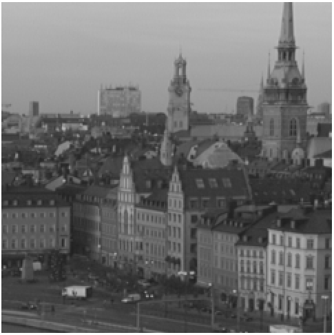
Refer to caption
(a) Source
Refer to caption
(b) Regular
Refer to caption
(c) Proposed
Figure 4: Coding a group of 10 frame from the ’Stockholm’ sequence (spatial portion of 480x480 pixels). (a) The third source frame. (b) the rendered frame using regular compression (28.29 dB at 2.37 bpp). (c) the rendered frame using the proposed compression (29.45 dB at 1.34 bpp).
Refer to caption
(a) Source
Refer to caption
(b) Regular
Refer to caption
(c) Proposed
Figure 5: Coding a group of 10 frame from the ’Shields’ sequence (spatial portion of 480x480 pixels). (a) The third source frame. (b) the rendered frame using regular compression (27.93 dB at 2.41 bpp). (c) the rendered frame using the proposed compression (29.31 dB at 1.31 bpp).