Understanding the interplay
between social and spatial behaviour

Abstract

According to personality psychology, personality traits determine many aspects of human behaviour. However, validating this insight in large groups has been challenging so far, due to the scarcity of multi-channel data. Here, we focus on the relationship between mobility and social behaviour by analysing trajectories and mobile phone interactions of $\sim 1,000$ individuals from two high-resolution longitudinal datasets. We identify a connection between the way in which individuals explore new resources and exploit known assets in the social and spatial spheres. We show that different individuals balance the exploration-exploitation trade-off in different ways and we explain part of the variability in the data by the big five personality traits. We point out that, in both realms, extraversion correlates with the attitude towards exploration and routine diversity, while neuroticism and openness account for the tendency to evolve routine over long time-scales. We find no evidence for the existence of classes of individuals across the spatio-social domains. Our results bridge the fields of human geography, sociology and personality psychology and can help improve current models of mobility and tie formation.

Introduction

Our social and spatial behaviour are shaped by both internal and external constraints. On one hand, external factors [1] such as time, cognition, age or the need for food constrain our possibilities. On the other hand, we are driven by internal needs, purposes and preferences. Specifically, within personality psychology, it has been conjectured that personality traits play a key role in shaping our choices across various situations [2, 3].

In the social realm, individuals cope with cognitive and temporal constraints by establishing and maintaining connections in a distinctive [4, 5] and persistent [4] manner. For example, the size of an individual’s social circle is bounded under $\sim 150$, the so-called Dunbar number [6], but varies among individuals around this limit [7]. These differences result from an interplay between physical and extrinsic factors such as gender [8], age [9] and socio-economic status [10] as well as from stable individual dispositions underlying personality [11].

Spatially, individuals are characterised by an activity space of repeatedly visited locations within which they move during their daily activities [12], but this geo-spatial signature varies in size [13] and spatial shape [14]. However, unlike the social case, the conjecture that individuals’ spatial behaviour is persistent in time [15] had not been verified until recently.

Here, we capitalise on the recent discovery that the size of the activity space is conserved and correlates with the social circle size [16] to test the conjecture that the same personality dispositions in part determine social and spatial behaviour. We test this theory by analysing two long-term datasets consisting of $\sim 1000$ individuals mobility trajectories and their phone interactions (for previous studies see section ‘State of the art’ below).

First, we test the hypothesis that the strategies individuals adopt in order to choose where to go and with whom to interact are similar. Then, we identify and characterise the prevailing socio-spatial profiles appearing in the datasets. Finally, we show that socio-spatial profiles can be partially explained by the widely adopted big-five personality trait model, often used to describe aspects of the social and emotional life [17, 18, 11, 7, 19, 20, 21, 22]. In the section ‘State of the art’, we review the relevant literature; in ‘Methods’ we describe data collection and pre-processing, and we provide details of the methods implemented; in ‘Results’ we present our findings.

State of the art

Individual-level variability in social and spatial behaviour has mostly been investigated in isolation so far, with few notable efforts to reconcile the two. Here, we briefly review the empirical findings in the two domains.

The social domain

Individuals deal with limited time and cognitive capacity resulting in finite social networks [6, 23] by distributing time unevenly across their social circle [24, 25, 26, 4, 27, 28]. While this is a shared strategy, there is clear evidence for individual-level variation. First, social circles vary in terms of diversity: they differ in size [7] - within a maximum upper-bound of $\sim 150$ individuals [6] - and in structure [4, 29]. Second, individuals display different attitudes towards exploration of social opportunities as they are more or less keen on creating new connections [30, 31, 32, 33]. Finally, individuals manage social interactions over time in different ways. Some are characterised by high level of stability as they maintain a very stable social circle, while others renew their social ties at high pace [5].

These heterogeneities can be partially explained by factors including gender [34, 8], age [9, 35, 36], socio-economic status [37, 10] and physical attractiveness [38]. Moreover, as conjectured by personality psychologists [39, 2], differences in personalities partially explain the variability in social circle composition [11, 7, 40, 17, 41, 42, 43, 44], and the different attitudes towards forming [30, 45], developing [46, 20] and replacing [29] social connections. It is worth noticing that many of these findings are recent, resulting from the analysis of digital communication traces.

The spatial domain

Constraints including physical capabilities, the distribution of resources, and the need to coordinate with others limit our possibilities to move in space [1]. Individuals cope with these limitations by allocating their time within an activity space of repeatedly visited locations [47], whose size is conserved over several years according to a recent study based on high-resolution trajectories [16], and previous ones based on unevenly sampled and low spatial resolution data [48, 49]. The activity space varies across individuals in terms of size [16] and shape [14]: it was shown that two distinct classes of individuals, returners and explorers, can be identified based on their propensity to visit new locations, similarly to the social domain [5]. Heterogeneities in spatial behaviour can be explained in terms of gender [50], age [51, 52], socio-economic [53, 35] and ethnic [54] differences. There has only been sporadic efforts to include personality measures in geographic research, despite the strong connections between the two [55]. Recent works [56, 44] suggest that spatial behaviour can be partially explained from personality traits. However, in [56], this understanding is based on biased data collected from location-based social networks. In [44], the connection between spatial behaviour and personality is not investigated extensively, as it is not the main focus of the study.

Social and spatial connection

Recently, connections between the social and spatial behaviour of pairs [57, 58, 59, 60, 61, 62] and groups [63] of individuals have been demonstrated, and used to design predictive models of mobility [58, 64, 65] or social ties [66, 59, 67, 68]. Shifting the attention to the individual level, recent works based on online social network data [69, 70], mobile phone calls data [62] and evenly sampled high resolution mobility trajectories [16] have shown correlations between the activity space size and the ego network structure, calling for further research to more closely examine the connections between social and spatial behaviour at the individual level.

Methods

Data description and pre-processing

Our study is based on $850$ high resolution trajectories and call records of participants in a $24$ months longitudinal experiment, the Copenhagen Networks Study (CNS) [71]. Results on the connections between social and spatial behaviour were corroborated with data from another experiment with fixed rate temporal sampling, but lower spatial resolution and sample size: the Lausanne Mobile Data Challenge (MDC) [72, 73], lasted for $19$ months (see Table 1).

	N	$\delta t$	$T$	$\delta x$	$TC$
CNS	850	16 s	24 months	10 m	0.84
MDC	185	60 s	19 months	100-200 m	0.73

Table 1: Characteristics of the mobility datasets considered. $N$ is the number of individuals, $\delta t$ the temporal resolution, $T$ the duration of data collection, $\delta x$ the spatial resolution, $TC$ the median weekly time coverage, defined as the fraction of time an individual’s location is known.

CNS dataset

The Copenhagen Networks Study (CNS) experiment took place between September 2013 and September 2015 [71] and involved $\sim 1000$ Technical University of Denmark students ($\sim 22\%$ female, $\sim 78\%$ male) typically aged between 19 and 21 years old. Participants’ position over time was estimated combining their smart-phones WiFi and GPS data using the method described in [74, 16]. The location estimation error is below 50 meters in 95% of the cases. Participants’ calls and sms activity was also collected as part of the experiment. Individuals’ background information were obtained through a 310 questions survey including the Big Five Inventory [75], which measures how individuals score on five broad domains of human personality traits: openness, conscientiousness, extraversion, agreeableness, neuroticism. The personality questionnaire used in the study is a version of the Big Five Inventory [75], translated from English into Danish. It contains 44 individual items and each trait is computed as the average of 7-10 items. Data collection was approved by the Danish Data Protection Agency. All participants provided individual informed consent. Mobility patterns of participants in the CNS experiment display statistical properties consistent with previous literature [13], as shown in [16].

MDC dataset

Data was collected by the Lausanne Data Collection Campaign between October 2009 and March 2011. The campaign involved an heterogeneous sample of $\sim 185$ volunteers with mixed backgrounds from the Lake Geneva region (Switzerland), who were allocated smart-phones [73]. In this work we used GSM data, that has the highest temporal sampling. Following Nokia’s privacy policy, individuals participating in the study provided informed consent [73]. The Lausanne Mobile Data Challenge experiment involves 62% male and 38% female participants, where the age range 22-33 year-old accounts for roughly 2/3 of the population [76].

Metrics

In this section, we define the concepts and metrics used to quantify the social and spatial behaviour of an individual $i$.

Exploration behaviour is characterised by the following quantities:

Number of new locations/week: $n_{loc}(i,t)$ is the number of locations discovered by $i$ in the week preceding $t$.

Number of new ties/week: $n_{tie}(i,t)$ is the number of individuals who had contact with $i$ (by sms or call) for the first time in the week preceding $t$.

Note that locations/ties are considered ‘new’ only if discovered after $20$ weeks from the beginning of data collection.

Exploitation behaviour can be quantified by considering:

Activity space: The set $AS(i,t)=\{\ell_{1},\ell_{2},...,\ell_{j},...\ell_{C}\}$ of locations $\ell_{j}$ that individual $i$ visited at least twice and where she spent a time $\tau_{j}$ larger than $200min$ during a time-window of $T=20$ weeks preceding time $t$ (see Supplementary Material for the analysis with $T=30$ weeks). Among the locations in the activity space, $i$ visited $\ell_{j}$ with probability $p(\ell_{j})=\tau_{j}/\sum\tau_{j}$. (It is worth noting that this time-based definition of activity space includes all significant locations independently of their spatial position and it is only loosely connected with space-oriented definitions widespread in the geography literature such as the “standard deviational ellipse” and the “road network buffer” [77]).

Social circle: The set $SC(i,t)=\{u_{1},u_{2},...,u_{j},...u_{k}\}$ of individuals $u_{j}$ with whom individual $i$ had a number of contacts $n_{j}>5$ by sms or call during a time-window of $T=20$ consecutive weeks preceding time $t$ (see Supplementary Material for the analysis with $T=30$ weeks). The probability that $i$ has contact with a given member $u_{j}$ of her social circle is $p(u_{j})=n_{j}/\sum n_{j}$.

For these two sets $AS(i,t)$ and $SC(i,t)$, we consider their sizes $C(i,t)$ and $k(i,t)$, quantifying the number of favoured locations and social ties, respectively; their entropies $H_{AS}(i,t)$ and $H_{SC}(i,t)$, measuring how time is allocated among locations and ties; their stabilities $J_{AS}(i,t)$ and $J_{SC}(i,t)$, quantifying the fraction of conserved locations and ties, respectively, across consecutive non-overlapping windows of $T=20$ weeks (see Supplementary Material for $T=30$); their rank turnovers $R_{AS}(i,t)$ and $R_{SC}(i,t)$ measuring the average absolute change in rank of an element in the set between consecutive windows. The mathematical definition of these quantities is provided in Table 2

	Activity space	Social circle
1) Size	$C(i,t)=|AS_{i}(t)|$	$k(i,t)=|SC(i,t)|$
2) Entropy	$H_{AS}(i,t)=-\sum\limits_{j=1}^{C(i,t)}{p(j)\log p(j)}$	$H_{SC}(i,t)=-\sum\limits_{j=1}^{k(i,t)}{p(j)\log p(j)}$
3) Stability	$J_{SC}(i,t)=\dfrac{|SC(i,t)\cap SC(i,t-T)|}{|SC(i,t)\cup SC(i,t-T)|}^{*}$	$J_{AS}(i,t)=\dfrac{|AS(i,t)\cap AS(i,t-T)|}{|AS(i,t)\cup AS(i,t-T)|}^{*}$
4) Rank       Turnover	$R_{AS}(i,t)=\sum\limits_{j=1}^{N}\dfrac{|r(j,t)-r(j,t-T)|^{**}}{N}$	$R_{SC}(i,t)=\sum\limits_{j=1}^{N}\dfrac{|r(j,t)-r(j,t-T)|^{**}}{N}$
∗ Here $T=20$ weeks, see Supplementary Material for the analysis with $T=30$ weeks
∗∗ $r(\ell_{k},t)$ and $r(u_{k},t)$ denote the rank of a location $\ell_{k}$ and individual $u_{k}$ at $t$, respectively

Table 2: Definition of the metrics characterising the activity space and the social circle. 1) The size of a set is the number of elements in the set 2) We compute the entropy of a set considering the probability $p(j)$ associated to each element $j$ of the set. 3) We measure the stability $J_{AS}$ by computing the Jaccard similarity between the activity space at $t$ and at $t-T$, with $T=20$ weeks. $J_{SC}$ is computed in the same way for the social circle. 4) We compute the rank turnover of a set by measuring for each of its elements $j$ the absolute change in rank between two consecutive time windows of length $T=20$ weeks. The rank is attributed based on the probability $p(j)$. The average absolute change in rank across all elements corresponds to the rank turnover.

.

Other metrics

In order to compare the difference in entropy between two different sets, we compute their Jensen-Shannon divergence (JSD). The JSD between two sets $P_{1}$ and $P_{2}$ is computed as $JSD(P_{1},P_{2})=H(\frac{1}{2}(P_{1}+P_{2}))-\frac{1}{2}[H(P_{1})+H(P_{2})]$ (see also [4]).

Results

Both in their spatial and social behaviour, individuals are constantly balancing a trade-off between the exploitation of familiar options (such as returning to a favourite restaurant or spending time with an old friend) and the exploration of new opportunities (such as visiting a new bar or going on a first date) [78]. We adopt this exploration-exploitation perspective to analyse the relationship between social and spatial strategies in our dataset [16].

We quantify the propensity for exploration and exploitation within each individual, $i$, using the metrics reported in Table 3, Fig. 1 and described in section ‘Methods’. We focus on two aspects of exploitation, (i) diversity, characterising how individuals allocate time among their set of familiar locations and friends, and (ii) evolution, characterising the tendency to change exploited locations and friends over time.

Figure 1: Schematic description of our framework.

	Exploration	Exploitation: Diversity	Exploitation: Evolution
Spatial	New loc./week, $n_{loc}$	Activity space size, $C$	Activity space stability, $J_{AS}$
		Activity space entropy, $H_{AS}$	Activity space rank turnover, $R_{AS}$
Social	New ties/week, $n_{tie}$	Social circle size, $k$	Social circle stability, $J_{SC}$
		Social circle entropy, $H_{SC}$	Social circle rank turnover, $R_{SC}$

Table 3: Metrics characterising social and spatial behaviour. The metrics are defined in section Methods

.

Exploration and exploitation are persistent in time. First, we verify that individual behaviour is persistent in time. For all the aforementioned measures, we compare the individual self-variation across time $d_{self}(i)$ with a reference difference $d_{ref}(i,j)$ between individuals $i$ and $j$. In the case of the activity space size, for example, self-variation is measured as $d_{self}=\langle|C(i,t)-C(i,t-T)|\rangle$, where $\langle\cdot\rangle$ is the average across time and $T=20$ weeks (see Supplementary Material for $T=30$) ; the reference difference is computed as $d_{ref}(i,j)=|\langle C(i,t)\rangle-\langle C(j,t)\rangle|$. If $d_{self}(i)<d_{ref}(i,j)$ for most $j$, we can conclude that for individual $i$, fluctuations of the activity space size are negligible compared to the difference with other individuals. The same procedure is followed for all metrics with an adjustment in the case of entropies: The persistence of the entropy $H_{AS}$ is verified by comparing the Janson-Shannon divergences $d_{self}=JSD(AS(i,t),AS(i,t-T))$ and $d_{ref}=JSD(AS(i,t),AS(j,t))$. The same method was used for $H_{SC}$ (see Methods and [4]).

Results from the CNS dataset reported in Table S3 show that for all metrics $d_{self}(i)<d_{ref}(i,j)$ holds in more than $99\%$ of cases on average (MDC: $97\%$, see Supplementary Material Table S1). Moreover, the average self-variation across the population $\overline{d_{self}}$ is consistent with $\overline{d_{self}}=0$ within errors, and $\overline{d_{self}}$ significantly smaller than the average reference difference $\overline{d_{ref}}$ (see Tables S3 and S1 in Supplementary Material).

	$\overline{d_{self}}$	$\overline{d_{ref}}$	$\overline{d_{self}(i)<d_{ref}(i,j)}$
Social circle size, $k$	$0.04\pm 0.09$	$12\pm 5$	$99$%
Activity space size, $C$	$0.04\pm 0.07$	$7\pm 3$	$99$%
New ties/week, $n_{tie}$	$0.05\pm 0.10$	$0.9\pm 0.5$	$96$%
New locations/week, $n_{loc}$	$0.10\pm 0.17$	$1\pm 1$	$95$%
Social circle entropy, $H_{SC}$	$0.002\pm 0.007$	$0.7\pm 0.2$	$99$%
Activity space entropy, $H_{AS}$	$0.002\pm 0.005$	$0.4\pm 0.1$	$99$%
Social circle stability, $J_{SC}$	$({9}\pm{22})\cdot 10^{-4}$	$0.13\pm 0.05$	$100$%
Activity space stability, $J_{AS}$	$({9}\pm{26})\cdot 10^{-4}$	$0.10\pm 0.04$	$99$%
Social circle rank turnover, $R_{SC}$	$0.05\pm 0.39$	$2\pm 1$	$99$%
Activity space rank turnover, $R_{AS}$	$0.04\pm 0.10$	$2\pm 1$	$99$%

Table 4: CNS dataset: Persistence of social and spatial behaviour.For each of the social and spatial metrics, $\overline{d_{self}}$ is the average self-distance and $\overline{d_{ref}}$ is the reference distance between an individual and all others, averaged across individuals. The third column reports the fraction of cases where $\overline{d_{self}(i)<d_{ref}(i,j)}$, averaged across the population.

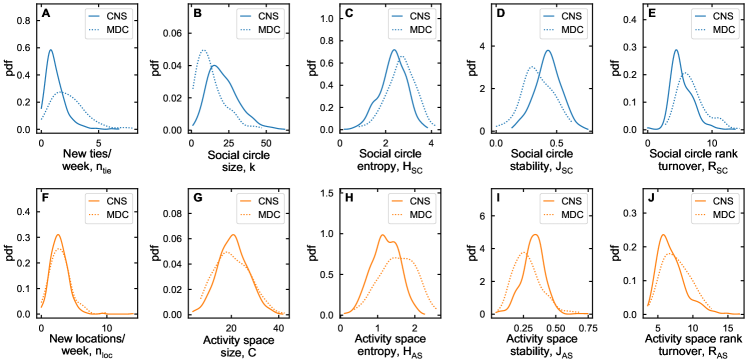
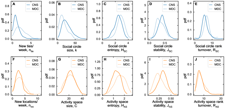
These results extend previous findings [4, 16] and suggest that each individual is characterised by a distinctive socio-spatial behaviour captured by the ensemble of these metrics averaged across time. In fact, these averages are heterogeneously distributed across the samples considered (see Fig. S2).

Figure 2: Distribution of social (above line) and spatial (bottom line) metrics for the CNS and MDC datasets.

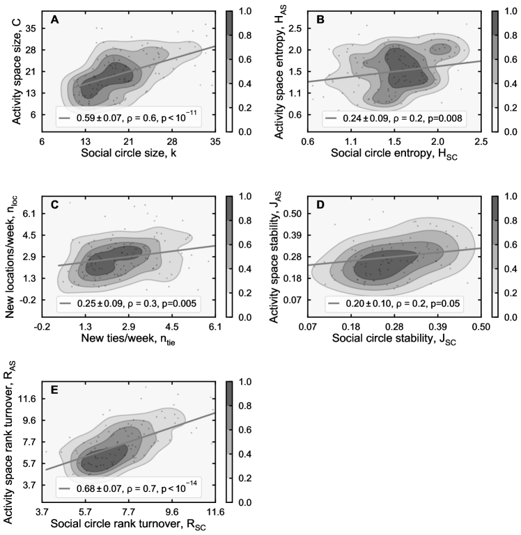
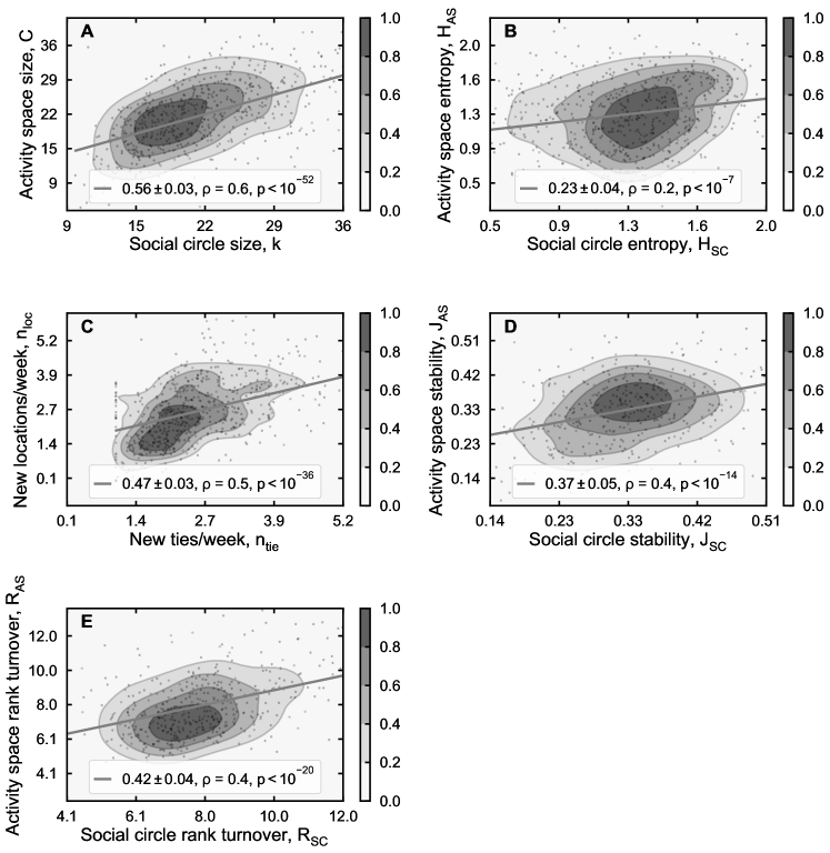
Exploration and exploitation are correlated in the social and spatial domain. A natural way to test the interdependency between social and spatial behaviours is measuring the correlation between a given social metric and a corresponding spatial one. We find positive and significant correlations for all metrics and datasets (see Figs. S3 and S1 in Supplementary Material).

Figure 3: CNS dataset: correlation between the four dimensions of social and spatial behaviour. (A) Activity space vs social circle size. (B) Activity space vs social circle composition measured as their entropy. (C) Average number of new locations vs new ties per week. (D) Stability of the activity space vs the stability of the social circle measured as the Jaccard similarity between their composition in consecutive time-windows. (E) Rank turnover of the activity space vs the rank turnover of the social circle. Coloured filled areas correspond to cumulative probabilities estimated via Gaussian Kernel Density estimations. Grey lines correspond to linear fit with angular coefficient $b$ reported in the legend. The Pearson correlation coefficient, with corresponding p-value, is reported in the legend.

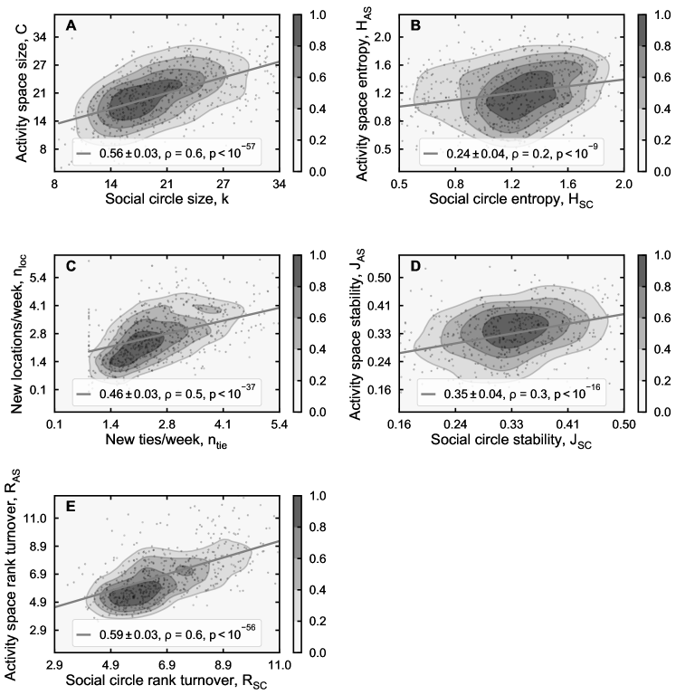
We find that individuals with high propensity to explore new locations are also more keen on exploring social opportunities (see Fig. S3A). Those with diverse mobility routine are also likely to have a correspondingly large social circle (see Fig. S3B), and those that often replace social ties, have also an unstable set of favourite locations (see Fig. S3C and D).

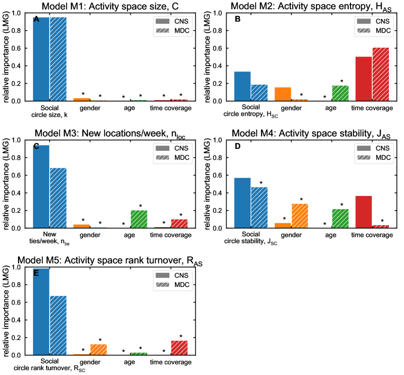
We verify that the observed correlations are not spurious by performing multiple regression analyses that control for other possible sources of variation: gender, age, and time coverage (the average time an individual position is known). We implement five multiple linear regression models M1, M2, M3, M4 and M5. Each regression model predicts a given spatial metric (the activity space size $C$, the activity space entropy $H_{AS}$, the number of new locations/week $n_{loc}$, the activity space stability $J_{AS}$ and the rank turnover $R_{AS}$) using the corresponding social metric and the control variables (age, gender and time coverage) as regressors. The relative importance of each regressor is assessed using the Lindeman, Merenda and Gold ($LMG$) [79] method.

Results obtained via weighted least square regression (see Tables S4 for the CNS dataset and S2 in Supplementary Material for the MDC dataset) reveal that the social metrics are significant predictors for spatial metrics (p value$<0.01$ in all cases except for M4 in the MDC dataset), and they typically have more importance than factors such as gender, time, coverage and age group (see Fig. S4).

Model M1: Activity space size, $C$	coeff	p val	LMG
Social circle size, $k$	$4\pm 0$	$<10^{-50}$	0.94
gender	$-0.4\pm 0.2$	0.05	0.05
time coverage	$0.4\pm 0.2$	0.06	0.01
[$R^{2}=0.32$, $F=100.44$, $p_{F}=0.0$ ]
Model M2: Activity space entropy, $H_{AS}$
Social circle entropy, $H_{SC}$	$0.07\pm 0.01$	$<10^{-6}$	0.42
gender	$-0.06\pm 0.01$	$<10^{-4}$	0.22
time coverage	$-0.07\pm 0.01$	$<10^{-5}$	0.36
[$R^{2}=0.11$, $F=27.30$, $p_{F}=0.0$]
Model M3: New locations/week, $n_{loc}$
New ties/week, $n_{tie}$	$0.60\pm 0.05$	$<10^{-32}$	0.9
gender	$-0.16\pm 0.05$	$<10^{-3}$	0.08
time coverage	$0.001\pm 0.047$	1.0	0.01
[$R^{2}=0.22$, $F=61.99$, $p_{F}=0.0$]
Model M4: Activity space stability, $J_{AS}$
Social circle stability, $J_{SC}$	$0.024\pm 0.004$	$<10^{-10}$	0.6
gender	$0.007\pm 0.003$	0.05	0.04
time coverage	$0.017\pm 0.004$	$<10^{-5}$	0.36
[$R^{2}=0.16$, $F=33.36$, $p_{F}=0.0$]
Model M5: Activity space rank turnover, $R_{AS}$
Social circle rank turnover, $R_{SC}$	$1\pm 0$	$<10^{-56}$	0.98
gender	$0.12\pm 0.07$	0.06	0.01
time coverage	$-0.12\pm 0.07$	0.07	0.01
[$R^{2}=0.36$, $F=108.31$, $p_{F}=0.0$]

Table 5: Linear regression models for the CNS dataset. For each model, we show the coefficients (coeff) calculated by the regression model, the probability (p val) that the variable is not relevant, and the relative importance (LMG) of each regressor computed using the Lindeman, Merenda and Gold method [79]. Gender is a binary variable taking value 1 for females and 2 for males. For this dataset, age is not relevant as all participants have similar age. For each model, we report the $R^{2}$ goodness of fit, the $F-test$ statistics with the corresponding p-value $p_{F}$.

Figure 4: Relative importance of regressors LMG of each regressor computed using the Lindeman, Merenda and Gold method [79] for models M1 (A), M2 (B), M3 (C), M4 (D) and M5 (D). Plain bars show results for the CNS dataset, dashed bars for the MDC dataset. Variables that are not significant in the regression model are marked with *.

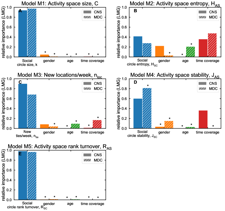
Among the control variables, gender is a significant predictor of spatial behaviour in the CNS dataset: Females display higher level of routine diversity and propensity towards exploration, in accordance with [80]. Time coverage, measuring the fraction of time an individual position is known, plays a significant role in explaining spatial entropy and activity space stability, since individuals who spend long time in the same place (or leave their phone in the same place) are more easily geo-localised. Age differences are not present within the sample of students participating in the CNS study, and they are not estimated to be relevant with respect to spatial behaviour in the MDC study.

We do not identify distinct classes of individuals. A natural question is whether or not, in the samples considered, there is evidence for distinct classes of individuals based on their socio-spatial behaviour [14, 5]. We approach this problem by reducing the set of metrics to a smaller number of uncorrelated variables by applying Principal Component Analysis [81, 82]. The principal components represent the data through linear combinations of the original variables: In Table 6 we report the percentage of variance in the data explained by all components; in Table 7 we report the coefficients $w$ describing how the original variables are linearly combined to obtain the first two principal components.

In both datasets, we find that the first principal component (PC 0) explains $\sim 40\%$ of the differences between individuals (see Table 6). For the CNS dataset, the variables contributing the most to PC 0 (e.g. such that $w^{2}>0.1$) are, in order, the activity space size $C$, the social circle size $k$, the number of new locations/week $n_{loc}$, the activity space entropy $H_{AS}$ and the number of new ties/week $n_{tie}$. $n_{loc}$ and $n_{tie}$ characterise the attitude towards exploration. The other metrics ($C$, $k$ and $H_{AS}$) are related to routine diversity, or the tendency to dispose of a large set of familiar locations and friends. Since the sign of $w$ is the same for all the metrics above, we can conclude that individuals with higher propensity towards exploration tend to have a more diverse social and spatial routine, and vice-versa. Similar conclusions could be drawn by looking at results obtained for the MDC dataset.

	PC 0	PC 1	PC 2	PC 3	PC 4	PC 5	PC 6	PC 7	PC 8	PC 9
CNS	0.39	0.17	0.12	0.08	0.07	0.06	0.04	0.03	0.03	0.01
MDC	0.43	0.14	0.13	0.08	0.07	0.06	0.04	0.03	0.02	0.01

Table 6: Variance explained by principal components. The fraction of variance explained by each principal component for the CNS and MDC dataset.

	CNS		MDC
	$w$ (PC 0)	$w$ (PC 1)	$w$ (PC 0)	$w$ (PC 1)
Social circle size, $k$	0.41	0.16	0.37	-0.15
Activity space size, $C$	0.42	-0.24	0.42	-0.08
New ties/week, $n_{tie}$	0.33	0.28	0.27	0.33
New locations/week, $n_{loc}$	0.38	-0.05	0.37	0.19
Social circle entropy, $H_{SC}$	0.31	0.30	0.34	0.09
Activity space entropy, $H_{AS}$	0.38	-0.16	0.30	-0.07
Social circle stability, $J_{SC}$	-0.16	-0.46	0.07	-0.72
Activity space stability, $J_{AS}$	-0.10	-0.49	-0.12	-0.51
Social circle rank turnover, $R_{SC}$	-0.20	0.28	-0.33	0.10
Activity space rank turnover, $R_{AS}$	-0.30	0.44	-0.38	0.17

Table 7: Contribution of the original variables to the first principal component. The scalar projection $w$ of the first (PC 0) and second (PC 1) principal components, along the axis defined by each of the original variables. Each principal component has unit norm, hence the sum of $w^{2}$ is $1$. Results are shown for the CNS and MDC datasets.

The second principal component (PC 1) accounts for $\sim 15\%$ of the total variation (see Table 6). It is dominated by the social circle stability $J_{SC}$ (CNS: $w^{2}=0.21$, MDC: $w^{2}=0.52$) and the activity space stability $J_{AS}$ (CNS: $w^{2}=0.24$, MDC: $w^{2}=0.26$) for both datasets (see Table 7). The sign of the coefficients $w$ for $J_{SC}$ and $J_{AS}$ are the same, further confirming that these two metrics are correlated (see also Fig. S3). We can conclude that the second principal component accounts for the effects of routine evolution, or the tendency to change familiar locations and friends over long time scales. We consider the first two principal components, PC 0 and PC 1, to reduce the effects of noise and we test the hypothesis that there exists different classes of individuals applying the gap statistic method [83]. We apply it by looking at the gap between the within-cluster dispersion expected under a uniform distribution of the data and the dispersion obtained after applying K-means. For all possible choices of $K>1$, we find that the gap is not large enough to support the existence of more than one class of individuals.

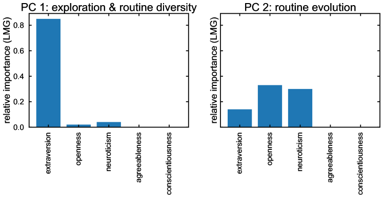
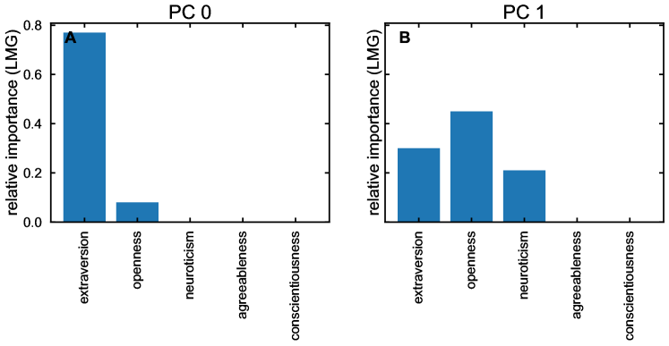
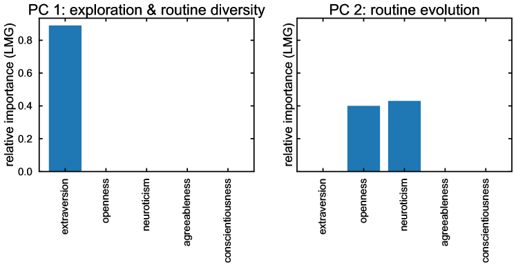
The big-five personality traits partly explain spatial and social behaviour. We verify if the differences between individuals can be explained by the Big five personality traits model [75], typically used to describe social and emotional life (see Table 8). We build two multiple linear regression models that use the Big five personality traits as regressors and one of the principal components describing socio-spatial behaviour as target. Results, shown in Table 9, show that three personality traits, neuroticism, openness and extraversion, are relevant predictors for socio-spatial behaviour. In particular, extraversion is the most important predictor of the first principal component: it positively correlates with the tendency to diversify routine and to explore opportunities. Neuroticism and openness explain instead the second principal component, since it correlates with the tendency to change routine over time (see also Fig. S5).

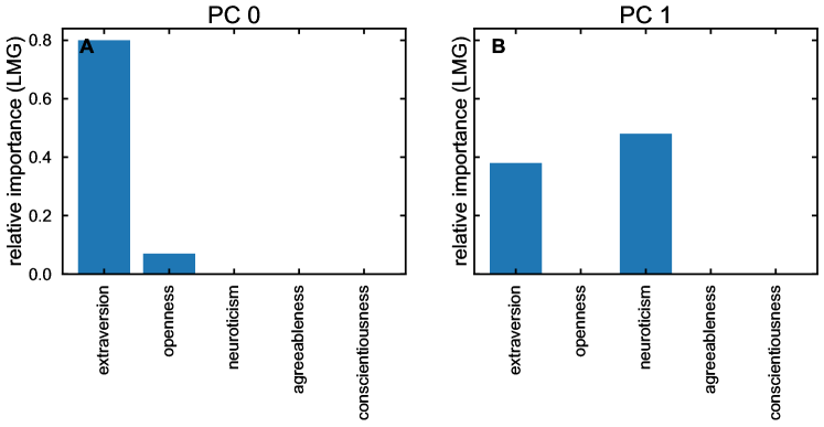
Finally, we perform all analyses considering only spatial metrics. Results are in line with those obtained considering all metrics: The first two principal components account for a large fraction of the variability in the data (see Table 10); The first component is dominated by the activity space size $C$, the number of new locations/week $n_{loc}$ and the activity space entropy $H_{AS}$, while the second is mostly controlled by the activity space stability $J_{AS}$ (Table 11). For the CNS dataset, extraversion is the most important predictor of the first principal component, while openness, extraversion and neuroticism account for the second component (see Table 12 and Fig. S6). The result presented above hold when choosing a time-window with length $T=30$ weeks (see Supplementary Material, section 2).

Trait	Related Adjectives
Extraversion	Active, Assertive, Energetic, Enthusiastic, Outgoing, Talkative
Agreeableness	Appreciative, Forgiving, Generous, Kind, Sympathetic
Conscientiousness	Efficient, Organised, Planful, Reliable, Responsible, Thorough
Neuroticism	Anxious, Self-pitying, Tense, Touchy, Unstable, Worrying
Openness to Experience	Artistic, Curious, Imaginative, Insightful, Original, Wide Interests

Table 8: The Big-Five traits and examples of adjectives describing them [84]

	PC 0 $R^{2}=0.17$, $F=21.40$, $p_{F}=0.0$			PC 1 $R^{2}=0.03$, $F=3.64$, $p_{F}=0.0$
	coeff	p val	LMG	coeff	p val	LMG
extraversion	$0.85\pm 0.09$	$<10^{-19}$	0.85	$0.12\pm 0.06$	0.05	0.14
openness	$-0.17\pm 0.08$	0.03	0.02	$0.13\pm 0.06$	0.02	0.33
neuroticism	$0.25\pm 0.09$	0.004	0.04	$0.15\pm 0.06$	0.02	0.3
agreeableness	$0.11\pm 0.08$	0.2	0.04	$-0.07\pm 0.06$	0.2	0.12
conscientiousness	$0.06\pm 0.08$	0.4	0.04	$-0.07\pm 0.06$	0.2	0.11

Table 9: Extraversion, openness, and neuroticism explain socio-spatial behaviour. The result of a multiple linear regression explaining principal components of socio-spatial data (see Table 7). The value of each coefficient (coeff) is reported together with the probability (p val) that the coefficient is not relevant for the model. The relative importance of each coefficient (LMG) is computed using the LMG method [79].

Figure 5: Relative importance of personality traits for socio-spatial behaviour LMG of each regressor computed using the Lindeman, Merenda and Gold method [79] for the multiple regression model of the principal components (see also Table 9).

Figure 6: Relative importance of personality traits for spatial behaviour LMG of each regressor computed using the Lindeman, Merenda and Gold method [79] for the multiple regression model of the principal components (see also Table 12).

	PC 0	PC 1	PC 2	PC 3	PC 4
CNS	0.53	0.21	0.13	0.10	0.04
MDC	0.56	0.19	0.13	0.07	0.04

Table 10: Variance explained by principal components (only spatial data). The fraction of variance explained by each principal component for the CNS and MDC dataset.

	CNS		MDC
	PC 0	PC 1	PC 0	PC 1
Activity space size, $C$	-0.58	0.02	0.55	0.12
New locations/week, $n_{loc}$	-0.48	-0.19	0.51	-0.09
Activity space entropy, $H_{AS}$	-0.50	-0.08	0.43	0.20
Activity space stability, $J_{AS}$	-0.02	0.94	-0.19	0.95
Activity space rank turnover, $R_{AS}$	0.43	-0.25	-0.47	-0.16

Table 11: Principal Components (only spatial data). The weight of each metric in the first two principal components, for both datasets.

	PC 0 $R^{2}=0.10$, $F=12.83$, $p_{F}=0.0$			PC 1 $R^{2}=0.03$, $F=3.50$, $p_{F}=0.0$
	coeff	p val	LMG	coeff	p val	LMG
extraversion	$-0.50\pm 0.07$	$<10^{-10}$	0.77	$-0.11\pm 0.05$	0.02	0.3
openness	$0.19\pm 0.07$	0.004	0.08	$-0.11\pm 0.04$	0.009	0.45
neuroticism	$-0.07\pm 0.07$	0.4	0.03	$-0.10\pm 0.05$	0.03	0.21
agreeableness	$-0.10\pm 0.07$	0.2	0.07	$0.01\pm 0.05$	0.8	0.01
conscientiousness	$-0.05\pm 0.07$	0.5	0.05	$0.03\pm 0.04$	0.4	0.03

Table 12: Extraversion, openness, and neuroticism explain spatial behaviour. The result of a multiple linear regression explaining principal components of spatial data (see Table 7). The value of each coefficient (coeff) is reported together with the probability (p val) that the coefficient is not relevant for the model. The relative importance of each coefficient (LMG) is computed using the LMG method [79].

Discussion

Using high resolution data from two large scale studies, we have investigated the connection between social and spatial behaviour for the first time. We have shown that, in both domains, individuals balance the trade-off between exploring new opportunities and exploiting known options in a distinctive and persistent manner. We have found that, to a significant extent, individuals adopt a similar strategy in the social and spatial sphere. These strategies are heterogeneous across the two samples considered, and there is no evidence suggesting that there exist distinct classes of individuals. Finally, we have shown that the big five personality traits explain related aspects of both social and spatial behaviour. In particular, we have found that extraverted individuals are more explorative and have diverse routines in both the social and the spatial sphere while neuroticism and openness associate with high level of routine instability in the social and spatial domain.

Our findings confirm the usefulness of mobile phone data to study the connections between behaviour and personality [85, 86, 40, 29, 44, 87]. The results are in line with previous findings on the relation between personality and social behaviour: extraversion correlates with ego-network size [43, 41, 18] and diverse composition [88], openness to experience to social network turnover [29] and neuroticism does not correlate with social network size [11]. Furthermore, our findings establish a relation between personality and spatial behaviour, validating the theories suggesting that spatial choices are partially dictated by personality dispositions [15] and that a single set of personality traits underlies many aspects of a person’s behaviour [2, 3].

Our findings on the connection between spatial behaviour and personality are consistent with the existing literature on personality. The correlation between exploration and extraversion could be explained by the fact that extraverted individuals are more likely to be risk-takers in various domains of life [89]. Extraverted individuals are also generally more likely to engage in social activities [90], which could partially explain why they allocate time among a larger set of locations. Furthermore, the key finding that individuals who score high in neuroticism and openness display a tendency to change familiar locations, and friends, over time fits well within the existing picture. In the case of neuroticism, it is well known that this trait is closely related with ‘stability’ [91], such that the trait of neuroticism is sometimes referred to as (low) ‘emotional stability’ [92]. Also, at the core of neuroticism is the tendency to experience negative emotions [93] including dissatisfaction [94], which in turn can lead into desire for change [95, 96]. Finally, it is known that people scoring high in neuroticism have a larger number of weak ties [42] and perceive that they tend to have less social support [97, 98], in line with our observation that they dispose of an unstable ego-network. Openness to experience has been shown to correlate with ‘disloyal’ behaviour also in other contexts such as politics [99] and shopping [100]. Our results, in agreement with previous studies on social [85, 86, 40, 29, 44, 87] and online [101, 102, 103, 104] behaviour, show that personality traits explain only partially how individuals behave in specific situations [105].

As a final point, we emphasize that the individual characterisation of spatial behaviour and connections with personality are fundamental to develop conceptual [55] and predictive [106] models of travel behaviour accounting for individual-level differences.

Competing interests

The authors declare that they have no competing interests.

Author’s contributions

LA, SL and AB designed the study; LA performed the analysis; LA, SL and AB analysed the results; LA, SL and AB wrote the paper.

List of Abbreviations

CNS: Copenhagen Networks Study
MDC: (Lausanne) Mobile Data Challenge
GSM: Global System for Mobile Communications
JSD: Jensen-Shannon divergence
LMG: Lindeman, Merenda and Gold

1 Results obtained with the MDC dataset

Tables S1, S2 and Fig. S1 report the results of the persistence analysis, the multiple regression analysis, and the correlation analysis for the MDC dataset.

	$\overline{d_{self}}$	$\overline{d_{ref}}$	$\overline{d_{self}(i)<d_{ref}(i,j)}$
Social circle size, $k$	$0.05\pm 0.13$	$10\pm 5$	$97$%
Activity space size, $C$	$0.07\pm 0.12$	$8\pm 3$	$97$%
New ties/week, $n_{tie}$	$0.2\pm 0.3$	$2\pm 1$	$91$%
New locations/week, $n_{loc}$	$0.2\pm 0.6$	$2\pm 1$	$90$%
Social circle entropy, $H_{SC}$	$0.006\pm 0.014$	$0.7\pm 0.3$	$97$%
Activity space entropy, $H_{AS}$	$0.004\pm 0.008$	$0.5\pm 0.2$	$97$%
Social circle stability, $J_{SC}$	$0.002\pm 0.005$	$0.15\pm 0.05$	$99$%
Activity space stability, $J_{AS}$	$0.002\pm 0.004$	$0.12\pm 0.05$	$99$%
Social circle rank turnover, $R_{SC}$	$0.07\pm 0.15$	$2\pm 1$	$98$%
Activity space rank turnover, $R_{AS}$	$0.2\pm 0.6$	$2\pm 1$	$97$%

Table S1: MDC dataset: Persistence of social and spatial behaviour. For each of the social and spatial metrics, $\overline{d_{self}}$ is the average self-distance and $\overline{d_{ref}}$ is the reference distance between an individual and all others, averaged across individuals. The third column reports the fraction of cases where $\overline{d_{self}(i)<d_{ref}(i,j)}$, averaged across the population.

Figure S1: MDC dataset: correlation between the four dimensions of social and spatial behaviour. (A) Activity space vs social circle size. (B) Activity space vs social circle composition measured as their entropy. (C) Average number of new locations vs new ties per week. (D) Stability of the activity space vs the stability of the social circle measured as the Jaccard similarity between their composition in consecutive time-windows. (E) Rank turnover of the activity space vs the rank turnover of the social circle. Coloured filled areas correspond to cumulative probabilities estimated via Gaussian Kernel Density estimations. Grey lines correspond to linear fit with angular coefficient $b$ reported in the legend. The Pearson correlation coefficient, with corresponding p-value, is reported in the legend.

Model M1: Activity space size, $C$	coeff	p val	LMG
Social circle size, $k$	$5\pm 1$	$<10^{-11}$	0.98
gender	$0.1\pm 0.6$	0.8	0.01
age group	$0.6\pm 0.6$	0.3	0.01
time coverage	$-0.4\pm 0.6$	0.4	0.0
[$R^{2}=0.40$, $F=16.80$, $p_{F}=0.0$]
Model M2: Activity space entropy, $H_{AS}$
Social circle entropy, $H_{SC}$	$0.11\pm 0.04$	0.009	0.28
gender	$0.04\pm 0.04$	0.3	0.03
age group	$-0.08\pm 0.04$	0.06	0.21
time coverage	$-0.14\pm 0.04$	0.002	0.48
[$R^{2}=0.20$, $F=6.50$, $p_{F}=0.0$]
Model M3: New locations/week, $n_{loc}$
New ties/week, $n_{tie}$	$0.5\pm 0.1$	0.002	0.69
gender	$0.01\pm 0.15$	0.9	0.04
age group	$0.2\pm 0.1$	0.2	0.1
time coverage	$-0.3\pm 0.1$	0.06	0.17
[$R^{2}=0.13$, $F=3.78$, $p_{F}=0.0$]
Model M4: Activity space stability, $J_{AS}$
Social circle stability, $J_{SC}$	$0.02\pm 0.01$	0.1	0.82
gender	$-0.006\pm 0.012$	0.6	0.15
age group	$-0.003\pm 0.012$	0.8	0.03
time coverage	$({-10}\pm{1213})\cdot 10^{-5}$	1.0	0.0
[$R^{2}=0.04$, $F=0.80$, $p_{F}=0.5$]
Model M5: Activity space rank turnover, $R_{AS}$
Social circle rank turnover, $R_{SC}$	$1\pm 0$	$<10^{-15}$	0.97
gender	$0.04\pm 0.15$	0.8	0.02
age group	$-0.2\pm 0.1$	0.1	0.01
time coverage	$-0.06\pm 0.15$	0.7	0.0
[$R^{2}=0.55$, $F=27.24$, $p_{F}=0.0$]

Table S2: Linear regression models for the MDC dataset. For each model, we report the $R^{2}$ goodness of fit, the $F-test$ statistics with the corresponfing p-value $p_{F}$. We show the coefficients (coeff) calculated by the regression model, the probability (p val) that the variable is not relevant, and the relative importance (LMG) of each regressor computed using the Lindeman, Merenda and Gold method. Gender is a binary variable taking value 1 for females and 2 for males.

2 Results obtained with other windows

Figs. S3, S5, S5, S6 and Tables S3, S4, S5, S6, S7, S8, S9, S10 report the results obtained choosing a time-window with length $T=30$ weeks (see main manuscript, section ‘Methods’).

Figure S2: T=30, Distribution of social (above line) and spatial (bottom line) metrics for the CNS and MDC datasets.

Figure S3: T=30, CNS dataset: correlation between the four dimensions of social and spatial behaviour. (A) Activity space vs social circle size. (B) Activity space vs social circle composition measured as their entropy. (C) Average number of new locations vs new ties per week. (D) Stability of the activity space vs the stability of the social circle measured as the Jaccard similarity between their composition in consecutive time-windows. (E) Rank turnover of the activity space vs the rank turnover of the social circle. Coloured filled areas correspond to cumulative probabilities estimated via Gaussian Kernel Density estimations. Grey lines correspond to linear fit with angular coefficient $b$ reported in the legend. The Pearson correlation coefficient, with corresponding p-value, is reported in the legend.

Figure S4: T=30, Relative importance of regressors LMG of each regressor computed using the Lindeman, Merenda and Gold method for models M1 (A), M2 (B), M3 (C), M4 (D) and M5 (E). Plain bars show results for the CNS dataset, dashed bars for the MDC dataset. Variables that are not significant in the regression model are marked with *.

Figure S5: T=30, Relative importance of personality traits for socio-spatial behaviour LMG of each regressor computed using the Lindeman, Merenda and Gold method for the multiple regression model of the principal components (table S7).

Figure S6: T=30, Relative importance of personalitry traits for spatial behaviour LMG of each regressor computed using the Lindeman, Merenda and Gold method for the multiple regression model of the principal components (table S10).

	$\overline{d_{self}}$	$\overline{d_{ref}}$	$\overline{d_{self}(i)<d_{ref}(i,j)}$
Social circle size, $k$	$0.04\pm 0.13$	$15\pm 6$	$100$%
Activity space size, $C$	$0.04\pm 0.07$	$8\pm 3$	$99$%
New ties/week, $n_{tie}$	$0.06\pm 0.12$	$0.9\pm 0.5$	$96$%
New locations/week, $n_{loc}$	$0.1\pm 0.2$	$1\pm 1$	$95$%
Social circle entropy, $H_{SC}$	$0.002\pm 0.005$	$0.7\pm 0.3$	$99$%
Activity space entropy, $H_{AS}$	$0.002\pm 0.006$	$0.4\pm 0.1$	$99$%
Social circle stability, $J_{SC}$	$({6}\pm{15})\cdot 10^{-4}$	$0.14\pm 0.05$	$100$%
Activity space stability, $J_{AS}$	$({6}\pm{11})\cdot 10^{-4}$	$0.10\pm 0.04$	$100$%
Social circle rank turnover, $R_{SC}$	$0.04\pm 0.11$	$2\pm 1$	$99$%
Activity space rank turnover, $R_{AS}$	$0.04\pm 0.20$	$2\pm 1$	$99$%

Table S3: T=30, CNS dataset: Persistence of social and spatial behaviour.For each of the social and spatial metrics, $\overline{d_{self}}$ is the average self-distance and $\overline{d_{ref}}$ is the reference distance between an individual and all others, averaged across individuals. The third column reports the fraction of cases where $\overline{d_{self}(i)<d_{ref}(i,j)}$, averaged across the population.

Model M1: Activity space size, $C$	coeff	p val	LMG
Social circle size, $k$	$4\pm 0$	$<10^{-46}$	0.95
gender	$-0.3\pm 0.2$	0.2	0.04
time coverage	$0.5\pm 0.2$	0.05	0.01
[$R^{2}=0.32$, $F=91.23$, $p_{F}=0.0$]
Model M2: Activity space entropy, $H_{AS}$
Social circle entropy, $H_{SC}$	$0.07\pm 0.02$	$<10^{-4}$	0.34
gender	$-0.05\pm 0.02$	$<10^{-3}$	0.16
time coverage	$-0.09\pm 0.02$	$<10^{-8}$	0.51
[$R^{2}=0.12$, $F=26.82$, $p_{F}=0.0$]
Model M3: New locations/week, $n_{loc}$
New ties/week, $n_{tie}$	$0.58\pm 0.05$	$<10^{-30}$	0.94
gender	$-0.09\pm 0.05$	0.04	0.04
time coverage	$0.03\pm 0.05$	0.5	0.01
[$R^{2}=0.22$, $F=55.56$, $p_{F}=0.0$]
Model M4: Activity space stability, $J_{AS}$
Social circle stability, $J_{SC}$	$0.027\pm 0.004$	$<10^{-9}$	0.57
gender	$0.009\pm 0.004$	0.02	0.06
time coverage	$0.020\pm 0.004$	$<10^{-5}$	0.37
[$R^{2}=0.18$, $F=30.32$, $p_{F}=0.0$]
Model M5: Activity space rank turnover, $R_{AS}$
Social circle rank turnover, $R_{SC}$	$0.81\pm 0.08$	$<10^{-19}$	0.99
gender	$0.09\pm 0.08$	0.3	0.01
time coverage	$-0.001\pm 0.084$	1.0	0.0
[$R^{2}=0.18$, $F=31.70$, $p_{F}=0.0$]

Table S4: T=30, Linear regression models for the CNS dataset. For each model, we report the $R^{2}$ goodness of fit, the $F-test$ statistics with the corresponfing p-value $p_{F}$. We show the coefficients (coeff) calculated by the regression model, the probability (p val) that the variable is not relevant, and the relative importance (LMG) of each regressor computed using the Lindeman, Merenda and Gold method. Gender is a binary variable taking value 1 for females and 2 for males. For this dataset, age is not relevant as all participants have similar age.

	PC 0	PC 1	PC 2	PC 3	PC 4	PC 5	PC 6	PC 7	PC 8	PC 9
CNS	0.40	0.18	0.10	0.07	0.07	0.06	0.04	0.03	0.03	0.02
MDC	0.39	0.19	0.12	0.10	0.06	0.05	0.05	0.03	0.02	0.01

Table S5: T=30, Variance explained by principal components. The fraction of variance explained by each principal component for the CNS and MDC dataset.

	CNS		MDC
	PC 0	PC 1	PC 0	PC 1
Social circle size, $k$	0.41	0.18	-0.36	0.04
Activity space size, $C$	0.42	-0.23	-0.40	-0.05
New ties/week, $n_{tie}$	0.33	0.27	-0.24	-0.35
New locations/week, $n_{loc}$	0.39	-0.11	-0.37	-0.22
Social circle entropy, $H_{SC}$	0.29	0.33	-0.36	-0.23
Activity space entropy, $H_{AS}$	0.38	-0.10	-0.35	0.13
Social circle stability, $J_{SC}$	-0.12	-0.50	-0.11	0.56
Activity space stability, $J_{AS}$	-0.06	-0.50	-0.03	0.62
Social circle rank turnover, $R_{SC}$	-0.17	0.26	0.28	-0.19
Activity space rank turnover, $R_{AS}$	-0.35	0.37	0.42	-0.18

Table S6: T=30, Principal Components. The weight of each metric in the first two principal components, for both datasets.

	PC 0 $R^{2}=0.17$, $F=17.08$, $p_{F}=0.0$			PC 1 $R^{2}=0.02$, $F=2.05$, $p_{F}=0.1$
	coeff	p val	LMG	coeff	p val	LMG
extraversion	$0.9\pm 0.1$	$<10^{-15}$	0.89	$0.06\pm 0.07$	0.4	0.04
openness	$-0.18\pm 0.09$	0.06	0.02	$0.13\pm 0.07$	0.05	0.4
neuroticism	$0.1\pm 0.1$	0.1	0.03	$0.15\pm 0.07$	0.04	0.43
agreeableness	$0.05\pm 0.10$	0.6	0.02	$-0.04\pm 0.07$	0.5	0.09
conscientiousness	$0.04\pm 0.10$	0.7	0.04	$-0.03\pm 0.07$	0.7	0.04

Table S7: T=30, Extraversion, openness, and neuroticism explain socio-spatial behaviour. The result of a multiple linear regression explaining principal components of socio-spatial data (Table S6). The value of each coefficient (coeff) is reported together with the probability (p val) that the coefficient is not relevant for the model. The relative importance of each coefficient (LMG) is computed using the LMG method.

	PC 0	PC 1	PC 2	PC 3	PC 4
CNS	0.57	0.21	0.10	0.08	0.04
MDC	0.55	0.24	0.12	0.06	0.03

Table S8: T=30, Variance explained by principal components (only spatial data). The fraction of variance explained by each principal component for the CNS and MDC dataset.

	CNS		MDC
	PC 0	PC 1	PC 0	PC 1
Activity space size, $C$	-0.55	0.01	-0.55	-0.10
New locations/week, $n_{loc}$	-0.48	-0.16	-0.48	-0.35
Activity space entropy, $H_{AS}$	-0.48	-0.14	-0.44	0.20
Activity space stability, $J_{AS}$	-0.06	0.96	-0.02	0.88
Activity space rank turnover, $R_{AS}$	0.48	-0.16	0.51	-0.22

Table S9: T=30, Principal Components (only spatial data). The weight of each metric in the first two principal components, for both datasets.

	PC 0 $R^{2}=0.11$, $F=11.55$, $p_{F}=0.0$			PC 1 $R^{2}=0.02$, $F=2.02$, $p_{F}=0.1$
	coeff	p val	LMG	coeff	p val	LMG
extraversion	$-0.56\pm 0.09$	$<10^{-9}$	0.8	$-0.12\pm 0.05$	0.03	0.38
openness	$0.20\pm 0.08$	0.01	0.07	$-0.04\pm 0.05$	0.5	0.08
neuroticism	$0.03\pm 0.08$	0.7	0.07	$-0.14\pm 0.05$	0.01	0.48
agreeableness	$-0.05\pm 0.08$	0.5	0.03	$-0.002\pm 0.052$	1.0	0.01
conscientiousness	$-0.005\pm 0.081$	1.0	0.03	$-0.03\pm 0.05$	0.6	0.04

Table S10: T=30, Extraversion, openness, and neuroticism explain spatial behaviour. The result of a multiple linear regression explaining principal components of spatial data (Table S6). The value of each coefficient (coeff) is reported together with the probability (p val) that the coefficient is not relevant for the model. The relative importance of each coefficient (LMG) is computed using the LMG method.

References

- [1] Torsten Hägerstraand. What about people in regional science? Papers in regional science, 24(1):7–24, 1970.
- [2] Walter Mischel. Toward a cognitive social learning reconceptualization of personality. Psychological review, 80(4):252, 1973.
- [3] Gordon Willard Allport. Personality: A psychological interpretation. 1937.
- [4] Jari Saramäki, Elizabeth A Leicht, Eduardo López, Sam GB Roberts, Felix Reed-Tsochas, and Robin IM Dunbar. Persistence of social signatures in human communication. Proceedings of the National Academy of Sciences, 111(3):942–947, 2014.
- [5] Giovanna Miritello, Rubén Lara, Manuel Cebrian, and Esteban Moro. Limited communication capacity unveils strategies for human interaction. Scientific reports, 3, 2013.
- [6] Robin IM Dunbar. Coevolution of neocortical size, group size and language in humans. Behavioral and brain sciences, 16(04):681–694, 1993.
- [7] Sam GB Roberts, Robin IM Dunbar, Thomas V Pollet, and Toon Kuppens. Exploring variation in active network size: Constraints and ego characteristics. Social Networks, 31(2):138–146, 2009.
- [8] Tasuku Igarashi, Jiro Takai, and Toshikazu Yoshida. Gender differences in social network development via mobile phone text messages: A longitudinal study. Journal of Social and Personal Relationships, 22(5):691–713, 2005.
- [9] Cornelia Wrzus, Martha Hänel, Jenny Wagner, and Franz J Neyer. Social network changes and life events across the life span: A meta-analysis. Psychological bulletin, 139(1):53, 2013.
- [10] Miller McPherson, Lynn Smith-Lovin, and Matthew E Brashears. Social isolation in america: Changes in core discussion networks over two decades. American sociological review, 71(3):353–375, 2006.
- [11] Sam GB Roberts, Ruth Wilson, Pawel Fedurek, and RIM Dunbar. Individual differences and personal social network size and structure. Personality and individual differences, 44(4):954–964, 2008.
- [12] Camille Perchoux, Basile Chaix, Steven Cummins, and Yan Kestens. Conceptualization and measurement of environmental exposure in epidemiology: accounting for activity space related to daily mobility. Health & place, 21:86–93, 2013.
- [13] Marta C Gonzalez, Cesar A Hidalgo, and Albert-Laszlo Barabasi. Understanding individual human mobility patterns. Nature, 453(7196):779–782, 2008.
- [14] Luca Pappalardo, Filippo Simini, Salvatore Rinzivillo, Dino Pedreschi, Fosca Giannotti, and Albert-László Barabási. Returners and explorers dichotomy in human mobility. Nature communications, 6, 2015.
- [15] Stuart C Aitken. Person-environment theories in contemporary perceptual and behavioural geography i: personality, attitudinal and spatial choice theories. Progress in Human Geography, 15(2):179–193, 1991.
- [16] Laura Alessandretti, Piotr Sapiezynski, Sune Lehmann, and Andrea Baronchelli. Evidence for a conserved quantity in human mobility. arXiv preprint arXiv:1609.03526, 2016.
- [17] Yu-En Lu, Sam Roberts, Pietro Lio, Robin Dunbar, and Jon Crowcroft. Size matters: variation in personal network size, personality and effect on information transmission. In Computational Science and Engineering, 2009. CSE’09. International Conference on, volume 4, pages 188–193. IEEE, 2009.
- [18] Tiziana Casciaro. Seeing things clearly: Social structure, personality, and accuracy in social network perception. Social Networks, 20(4):331–351, 1998.
- [19] Mohammadreza Hojat. Loneliness as a function of selected personality variables. Journal of Clinical Psychology, 38(1):137–141, 1982.
- [20] Susan JT Branje, Cornelis FM van Lieshout, and Marcel AG van Aken. Relations between big five personality characteristics and perceived support in adolescents’ families. Journal of personality and social psychology, 86(4):615, 2004.
- [21] Paul R Amato. Personality and social network involvement as predictors of helping behavior in everyday life. Social Psychology Quarterly, pages 31–43, 1990.
- [22] Yair Amichai Hamburger and Elisheva Ben-Artzi. The relationship between extraversion and neuroticism and the different uses of the internet. Computers in human behavior, 16(4):441–449, 2000.
- [23] Bruno Gonçalves, Nicola Perra, and Alessandro Vespignani. Modeling users’ activity on twitter networks: Validation of dunbar’s number. PloS one, 6(8):e22656, 2011.
- [24] Alistair Sutcliffe, Robin Dunbar, Jens Binder, and Holly Arrow. Relationships and the social brain: integrating psychological and evolutionary perspectives. British journal of psychology, 103(2):149–168, 2012.
- [25] Valerio Arnaboldi, Marco Conti, Andrea Passarella, and Fabio Pezzoni. Analysis of ego network structure in online social networks. In Privacy, security, risk and trust (PASSAT), 2012 international conference on and 2012 international confernece on social computing (SocialCom), pages 31–40. IEEE, 2012.
- [26] Giovanna Miritello, Esteban Moro, Rubén Lara, Rocío Martínez-López, John Belchamber, Sam GB Roberts, and Robin IM Dunbar. Time as a limited resource: Communication strategy in mobile phone networks. Social Networks, 35(1):89–95, 2013.
- [27] W-X Zhou, Didier Sornette, Russell A Hill, and Robin IM Dunbar. Discrete hierarchical organization of social group sizes. Proceedings of the Royal Society of London B: Biological Sciences, 272(1561):439–444, 2005.
- [28] Cameron Marlow, L Byron, T Lento, and I Rosenn. Maintained relationships on facebook. Retrieved February, 15(8), 2009.
- [29] Simone Centellegher, Eduardo López, Jari Saramäki, and Bruno Lepri. Personality traits and ego-network dynamics. PloS one, 12(3):e0173110, 2017.
- [30] Stefan Wehrli et al. Personality on social network sites: An application of the five factor model. Zurich: ETH Sociology (Working Paper No. 7), 2008.
- [31] Ravi Kumar, Jasmine Novak, and Andrew Tomkins. Structure and evolution of online social networks. In Link mining: models, algorithms, and applications, pages 337–357. Springer, 2010.
- [32] Mark EJ Newman. Clustering and preferential attachment in growing networks. Physical review E, 64(2):025102, 2001.
- [33] Alan Mislove, Hema Swetha Koppula, Krishna P Gummadi, Peter Druschel, and Bobby Bhattacharjee. Growth of the flickr social network. In Proceedings of the first workshop on Online social networks, pages 25–30. ACM, 2008.
- [34] Robin IM Dunbar and Matt Spoors. Social networks, support cliques, and kinship. Human nature, 6(3):273–290, 1995.
- [35] Juan Carrasco, Eric Miller, and Barry Wellman. How far and with whom do people socialize?: Empirical evidence about distance between social network members. Transportation Research Record: Journal of the Transportation Research Board, (2076):114–122, 2008.
- [36] Pauline van den Berg, Theo Arentze, and Harry Timmermans. Size and composition of ego-centered social networks and their effect on geographic distance and contact frequency. Transportation Research Record: Journal of the Transportation Research Board, (2135):1–9, 2009.
- [37] Karen E Campbell, Peter V Marsden, and Jeanne S Hurlbert. Social resources and socioeconomic status. Social networks, 8(1):97–117, 1986.
- [38] Harry T Reis, John Nezlek, and Ladd Wheeler. Physical attractiveness in social interaction. Journal of Personality and Social Psychology, 38(4):604, 1980.
- [39] James J Jaccard. Predicting social behavior from personality traits. Journal of Research in Personality, 7(4):358–367, 1974.
- [40] Jacopo Staiano, Bruno Lepri, Nadav Aharony, Fabio Pianesi, Nicu Sebe, and Alex Pentland. Friends don’t lie: inferring personality traits from social network structure. In Proceedings of the 2012 ACM conference on ubiquitous computing, pages 321–330. ACM, 2012.
- [41] Jens B Asendorpf and Marcel AG Van Aken. Personality–relationship transaction in adolescence: Core versus surface personality characteristics. Journal of personality, 71(4):629–666, 2003.
- [42] Yuval Kalish and Garry Robins. Psychological predispositions and network structure: The relationship between individual predispositions, structural holes and network closure. Social networks, 28(1):56–84, 2006.
- [43] Thomas V Pollet, Sam GB Roberts, and Robin IM Dunbar. Extraverts have larger social network layers. Journal of Individual Differences, 2011.
- [44] Yves-Alexandre de Montjoye, Jordi Quoidbach, Florent Robic, and Alex Pentland. Predicting personality using novel mobile phone-based metrics. In SBP, pages 48–55. Springer, 2013.
- [45] Maarten Selfhout, William Burk, Susan Branje, Jaap Denissen, Marcel Van Aken, and Wim Meeus. Emerging late adolescent friendship networks and big five personality traits: A social network approach. Journal of personality, 78(2):509–538, 2010.
- [46] Jens Asendorpf and Jaap JA Denissen. Predictive validity of personality types versus personality dimensions from early childhood to adulthood: Implications for the distinction between core and surface traits. Merrill-Palmer Quarterly, 52(3):486–513, 2006.
- [47] Reginald G Golledge. Spatial behavior: A geographic perspective. Guilford Press, 1997.
- [48] Olle Järv, Rein Ahas, and Frank Witlox. Understanding monthly variability in human activity spaces: A twelve-month study using mobile phone call detail records. Transportation Research Part C: Emerging Technologies, 38:122–135, 2014.
- [49] Stefan Schönfelder and Kay W Axhausen. Urban rhythms and travel behaviour: spatial and temporal phenomena of daily travel. Ashgate Publishing, Ltd., 2010.
- [50] Mei-Po Kwan. Gender differences in space-time constraints. Area, 32(2):145–156, 2000.
- [51] Gonzalo M Vazquez-Prokopec, Donal Bisanzio, Steven T Stoddard, Valerie Paz-Soldan, Amy C Morrison, John P Elder, Jhon Ramirez-Paredes, Eric S Halsey, Tadeusz J Kochel, Thomas W Scott, et al. Using gps technology to quantify human mobility, dynamic contacts and infectious disease dynamics in a resource-poor urban environment. PloS one, 8(4):e58802, 2013.
- [52] Chaogui Kang, Song Gao, Xing Lin, Yu Xiao, Yihong Yuan, Yu Liu, and Xiujun Ma. Analyzing and geo-visualizing individual human mobility patterns using mobile call records. In Geoinformatics, 2010 18th International Conference on, pages 1–7. IEEE, 2010.
- [53] Shannon N Zenk, Amy J Schulz, Stephen A Matthews, Angela Odoms-Young, JoEllen Wilbur, Lani Wegrzyn, Kevin Gibbs, Carol Braunschweig, and Carmen Stokes. Activity space environment and dietary and physical activity behaviors: a pilot study. Health & place, 17(5):1150–1161, 2011.
- [54] Mei-Po Kwan and Jiyeong Lee. Geovisualization of human activity patterns using 3d gis: a time-geographic approach. Spatially integrated social science, 27, 2004.
- [55] Veronique Van Acker, Bert Van Wee, and Frank Witlox. When transport geography meets social psychology: toward a conceptual model of travel behaviour. Transport Reviews, 30(2):219–240, 2010.
- [56] Martin J Chorley, Roger M Whitaker, and Stuart M Allen. Personality and location-based social networks. Computers in Human Behavior, 46:45–56, 2015.
- [57] Lars Backstrom, Eric Sun, and Cameron Marlow. Find me if you can: improving geographical prediction with social and spatial proximity. In Proceedings of the 19th international conference on World wide web, pages 61–70. ACM, 2010.
- [58] Jeffrey McGee, James Caverlee, and Zhiyuan Cheng. Location prediction in social media based on tie strength. In Proceedings of the 22nd ACM international conference on Information & Knowledge Management, pages 459–468. ACM, 2013.
- [59] Adam Sadilek, Henry Kautz, and Jeffrey P Bigham. Finding your friends and following them to where you are. In Proceedings of the fifth ACM international conference on Web search and data mining, pages 723–732. ACM, 2012.
- [60] David J Crandall, Lars Backstrom, Dan Cosley, Siddharth Suri, Daniel Huttenlocher, and Jon Kleinberg. Inferring social ties from geographic coincidences. Proceedings of the National Academy of Sciences, 107(52):22436–22441, 2010.
- [61] Przemyslaw A Grabowicz, Jose J Ramasco, Bruno Gonçalves, and Víctor M Eguíluz. Entangling mobility and interactions in social media. PloS one, 9(3):e92196, 2014.
- [62] Jameson L Toole, Carlos Herrera-Yaqüe, Christian M Schneider, and Marta C González. Coupling human mobility and social ties. Journal of The Royal Society Interface, 12(105):20141128, 2015.
- [63] Jukka-Pekka Onnela, Samuel Arbesman, Marta C González, Albert-László Barabási, and Nicholas A Christakis. Geographic constraints on social network groups. PLoS one, 6(4):e16939, 2011.
- [64] David Jurgens. That’s what friends are for: Inferring location in online social media platforms based on social relationships. ICWSM, 13(13):273–282, 2013.
- [65] Eunjoon Cho, Seth A Myers, and Jure Leskovec. Friendship and mobility: user movement in location-based social networks. In Proceedings of the 17th ACM SIGKDD international conference on Knowledge discovery and data mining, pages 1082–1090. ACM, 2011.
- [66] Dashun Wang, Dino Pedreschi, Chaoming Song, Fosca Giannotti, and Albert-Laszlo Barabasi. Human mobility, social ties, and link prediction. In Proceedings of the 17th ACM SIGKDD international conference on Knowledge discovery and data mining, pages 1100–1108. ACM, 2011.
- [67] Salvatore Scellato, Anastasios Noulas, and Cecilia Mascolo. Exploiting place features in link prediction on location-based social networks. In Proceedings of the 17th ACM SIGKDD international conference on Knowledge discovery and data mining, pages 1046–1054. ACM, 2011.
- [68] Huy Pham, Cyrus Shahabi, and Yan Liu. Ebm: an entropy-based model to infer social strength from spatiotemporal data. In Proceedings of the 2013 ACM SIGMOD International Conference on Management of Data, pages 265–276. ACM, 2013.
- [69] Zhiyuan Cheng, James Caverlee, Kyumin Lee, and Daniel Z Sui. Exploring millions of footprints in location sharing services. ICWSM, 2011:81–88, 2011.
- [70] Justin Cranshaw, Eran Toch, Jason Hong, Aniket Kittur, and Norman Sadeh. Bridging the gap between physical location and online social networks. In Proceedings of the 12th ACM international conference on Ubiquitous computing, pages 119–128. ACM, 2010.
- [71] Arkadiusz Stopczynski, Vedran Sekara, Piotr Sapiezynski, Andrea Cuttone, Mette My Madsen, Jakob Eg Larsen, and Sune Lehmann. Measuring large-scale social networks with high resolution. PloS one, 9(4):e95978, 2014.
- [72] Niko Kiukkonen, Jan Blom, Olivier Dousse, Daniel Gatica-Perez, and Juha Laurila. Towards rich mobile phone datasets: Lausanne data collection campaign. Proc. ICPS, Berlin, 2010.
- [73] Juha K Laurila, Daniel Gatica-Perez, Imad Aad, Olivier Bornet, Trinh-Minh-Tri Do, Olivier Dousse, Julien Eberle, Markus Miettinen, et al. The mobile data challenge: Big data for mobile computing research. In Pervasive Computing, number EPFL-CONF-192489, 2012.
- [74] Piotr Sapiezynski, Radu Gatej, Alan Mislove, and Sune Lehmann. Opportunities and challenges in crowdsourced wardriving. In Proceedings of the 2015 ACM Conference on Internet Measurement Conference, pages 267–273. ACM, 2015.
- [75] Oliver P John and Sanjay Srivastava. The big five trait taxonomy: History, measurement, and theoretical perspectives. Handbook of personality: Theory and research, 2(1999):102–138, 1999.
- [76] Juha K Laurila, Daniel Gatica-Perez, Imad Aad, Jan Blom, Olivier Bornet, Trinh Minh Tri Do, Olivier Dousse, Julien Eberle, and Markus Miettinen. From big smartphone data to worldwide research: The mobile data challenge. Pervasive and Mobile Computing, 9(6):752–771, 2013.
- [77] Jill E Sherman, John Spencer, John S Preisser, Wilbert M Gesler, and Thomas A Arcury. A suite of methods for representing activity space in a healthcare accessibility study. International journal of health geographics, 4(1):24, 2005.
- [78] Thomas T Hills, Peter M Todd, David Lazer, A David Redish, Iain D Couzin, Cognitive Search Research Group, et al. Exploration versus exploitation in space, mind, and society. Trends in cognitive sciences, 19(1):46–54, 2015.
- [79] Ulrike Grömping et al. Relative importance for linear regression in r: the package relaimpo. Journal of statistical software, 17(1):1–27, 2006.
- [80] Anders Mollgaard, Sune Lehmann, and Joachim Mathiesen. Correlations between human mobility and social interaction reveal general activity patterns. PloS one, 12(12):e0188973, 2017.
- [81] Svante Wold, Kim Esbensen, and Paul Geladi. Principal component analysis. Chemometrics and intelligent laboratory systems, 2(1-3):37–52, 1987.
- [82] Sebastian Mika, Bernhard Schölkopf, Alex J Smola, Klaus-Robert Müller, Matthias Scholz, and Gunnar Rätsch. Kernel pca and de-noising in feature spaces. In Advances in neural information processing systems, pages 536–542, 1999.
- [83] Robert Tibshirani, Guenther Walther, and Trevor Hastie. Estimating the number of clusters in a data set via the gap statistic. Journal of the Royal Statistical Society: Series B (Statistical Methodology), 63(2):411–423, 2001.
- [84] Robert R McCrae and Oliver P John. An introduction to the five-factor model and its applications. Journal of personality, 60(2):175–215, 1992.
- [85] Renaud Lambiotte and Michal Kosinski. Tracking the digital footprints of personality. Proceedings of the IEEE, 102(12):1934–1939, 2014.
- [86] Andrey Bogomolov, Bruno Lepri, Michela Ferron, Fabio Pianesi, and Alex Sandy Pentland. Daily stress recognition from mobile phone data, weather conditions and individual traits. In Proceedings of the 22nd ACM international conference on Multimedia, pages 477–486. ACM, 2014.
- [87] Gokul Chittaranjan, Jan Blom, and Daniel Gatica-Perez. Mining large-scale smartphone data for personality studies. Personal and Ubiquitous Computing, 17(3):433–450, 2013.
- [88] Adrien Friggeri, Renaud Lambiotte, Michal Kosinski, and Eric Fleury. Psychological aspects of social communities. In Privacy, Security, Risk and Trust (PASSAT), 2012 International Conference on and 2012 International Confernece on Social Computing (SocialCom), pages 195–202. IEEE, 2012.
- [89] Nigel Nicholson, Emma Soane, Mark Fenton-O’Creevy, and Paul Willman. Personality and domain-specific risk taking. Journal of Risk Research, 8(2):157–176, 2005.
- [90] Richard E Lucas, Ed Diener, Alexander Grob, Eunkook M Suh, and Liang Shao. Cross-cultural evidence for the fundamental features of extraversion. Journal of personality and social psychology, 79(3):452, 2000.
- [91] Michael D Robinson and Maya Tamir. Neuroticism as mental noise: a relation between neuroticism and reaction time standard deviations. Journal of Personality and Social Psychology, 89(1):107, 2005.
- [92] Timothy A Judge and Joyce E Bono. Relationship of core self-evaluations traits—self-esteem, generalized self-efficacy, locus of control, and emotional stability—with job satisfaction and job performance: A meta-analysis. Journal of applied Psychology, 86(1):80, 2001.
- [93] Paul T Costa and Robert R McCrea. Revised neo personality inventory (neo pi-r) and neo five-factor inventory (neo-ffi). Psychological Assessment Resources, 1992.
- [94] Paul T Costa and Robert R McCrae. Influence of extraversion and neuroticism on subjective well-being: happy and unhappy people. Journal of personality and social psychology, 38(4):668, 1980.
- [95] Jing Zhou and Jennifer M George. When job dissatisfaction leads to creativity: Encouraging the expression of voice. Academy of Management journal, 44(4):682–696, 2001.
- [96] Caryl E Rusbult and Isabella M Zembrodt. Responses to dissatisfaction in romantic involvements: A multidimensional scaling analysis. Journal of Experimental Social Psychology, 19(3):274–293, 1983.
- [97] Daniel W Russell, Brenda Booth, David Reed, and Philip R Laughlin. Personality, social networks, and perceived social support among alcoholics: A structural equation analysis. Journal of Personality, 65(3):649–692, 1997.
- [98] Joseph P Stokes. The relation of social network and individual difference variables to loneliness. Journal of Personality and Social Psychology, 48(4):981, 1985.
- [99] Bert N Bakker, Robert Klemmensen, Asbjørn Sonne Nørgaard, and Gijs Schumacher. Stay loyal or exit the party? how openness to experience and extroversion explain vote switching. Political Psychology, 37(3):419–429, 2016.
- [100] Kurt Matzler, Sonja Bidmon, and Sonja Grabner-Kräuter. Individual determinants of brand affect: the role of the personality traits of extraversion and openness to experience. Journal of Product & Brand Management, 15(7):427–434, 2006.
- [101] Yoram Bachrach, Michal Kosinski, Thore Graepel, Pushmeet Kohli, and David Stillwell. Personality and patterns of facebook usage. In Proceedings of the 4th Annual ACM Web Science Conference, pages 24–32. ACM, 2012.
- [102] Dejan Markovikj, Sonja Gievska, Michal Kosinski, and David Stillwell. Mining facebook data for predictive personality modeling. In Proceedings of the 7th international AAAI conference on Weblogs and Social Media (ICWSM 2013), Boston, MA, USA, pages 23–26, 2013.
- [103] Daniele Quercia, Michal Kosinski, David Stillwell, and Jon Crowcroft. Our twitter profiles, our selves: Predicting personality with twitter. In Privacy, Security, Risk and Trust (PASSAT) and 2011 IEEE Third Inernational Conference on Social Computing (SocialCom), 2011 IEEE Third International Conference on, pages 180–185. IEEE, 2011.
- [104] Michal Kosinski, David Stillwell, and Thore Graepel. Private traits and attributes are predictable from digital records of human behavior. Proceedings of the National Academy of Sciences, 110(15):5802–5805, 2013.
- [105] William Fleeson and Erik Noftle. The end of the person–situation debate: An emerging synthesis in the answer to the consistency question. Social and Personality Psychology Compass, 2(4):1667–1684, 2008.
- [106] Shan Jiang, Yingxiang Yang, Siddharth Gupta, Daniele Veneziano, Shounak Athavale, and Marta C González. The timegeo modeling framework for urban motility without travel surveys. Proceedings of the National Academy of Sciences, page 201524261, 2016.
Supplementary Material for
Understanding the interplay between social and spatial behaviour