Model-Based Action Exploration for Learning Dynamic Motion Skills

Abstract

Deep reinforcement learning has achieved great strides in solving challenging motion control tasks. Recently, there has been significant work on methods for exploiting the data gathered during training, but there has been less work on how to best generate the data to learn from. For continuous action domains, the most common method for generating exploratory actions involves sampling from a Gaussian distribution centred around the mean action output by a policy. Although these methods can be quite capable, they do not scale well with the dimensionality of the action space, and can be dangerous to apply on hardware. We consider learning a forward dynamics model to predict the result, ($x_{t+1}$), of taking a particular action, ($u$), given a specific observation of the state, ($x_{t}$). With this model we perform internal look-ahead predictions of outcomes and seek actions we believe have a reasonable chance of success. This method alters the exploratory action space, thereby increasing learning speed and enables higher quality solutions to difficult problems, such as robotic locomotion and juggling.

Efficient action exploration remains a challenge for Rienforcement Learning (RL), especially in continuous action domains. Gaussian distributions are commonly used to model the stochastic component of control policies in continuous action spaces. However, as the number of action dimensions increase the probability of randomly generating an action that is better than the current policy decreases exponentially with the action dimension.

Recent work has indicated that methods that add local noise might not be enough to explore environments well [1]. Other methods model the action distribution better by learning a noise distribution [2] or processing random Gaussian noise through the policy [3]. However, these methods may not scale well with respect to the number of action dimensions. In practise, we expect that there likely exists better distributions that will focus the sampled actions to areas of the action space that appear more promising. This is of particular importance to problems where data collection is expensive, like robotics.

We want to generate exploratory actions that have a greater probability of leading the policy to higher value states. We do this in a model-based way, using a learned model of the environment’s transition probability $\hat{P}(x_{t+1}|x_{t},u_{t},\theta_{\hat{P}})$. The model is used to predict outcomes of taking actions in particular states. Predicted states are rated, via the value function, for how well it is believed the policy will perform from that state onward. This method is similar to how a person might use an internal understanding of the result of taking an action and modifying that action to increase the utility (or cumulative reward) of their future. We call this method Model-Based Action Exploration (MBAE). This work is a step towards mixing model-based and model-free learning. We use a model-based method to assist action exploration and model-free methods for training. We note that MBAE should be used in conjunction with off-policy algorithms.

Our work is motivated by the desire to solve more complex simulated and robotic tasks. The mathematical framework is inspired by Deterministic Policy Gradient (DPG) [4] where action gradients can be computed for the policy given an action-value (Q) function However, in practise these gradients are noisy and can vary greatly in their magnitude. This can make it challenging to create a stable learning framework. In a sense, in MBAE we are passing these gradients through the environment as an extra means of validation, thereby decreasing the bias and increasing the stability of learning. This work is also motivated by the idea that the significant body of data collected while training an RL policy should be leveraged for additional purposes.

(a) Membrane Hardware

(b) Membrane Simulation

Figure 1: (a) The Membrane robot. The blue points between the parallel links are actuated up and down via the servos on the bottom. Each point is connected together with a passive slider, together they form a Membrane-like system. Right: Simulated model of Membrane robot.

I Related Work

Reinforcement Learning

The environment in a RL problem is often modelled as an Markov Dynamic Processes (MDP) with a discrete set of states and actions [5]. In this work we are focusing on problems with infinite/continuous state and action spaces. These include complex motor control tasks that have become a popular benchmark in the machine learning literature [6]. Many recent RL approaches are based on policy gradient methods [7] where the gradient of the policy with respect to future discounted reward is approximated and used to update the policy. Recent advances in combining policy gradient methods and deep learning have led to impressive results for numerous problems, including Atari games and bipedal motion control [8, 9, 10, 11, 12, 13].

Sample Efficient RL

While policy gradient methods provide a general framework for how to update a policy given data, it is still a challenge to generate good data. Sample efficient RL methods are an important area of research as learning complex policies for motion control can take days and physically simulating on robots is time-consuming. Learning can be made more sample efficient by further parameterizing the policy and passing noise through the network as an alternative to adding vanilla Gaussian noise [3, 2]. Other work encourages exploration of the state space that has not yet been seen by the agent [14]. There has been success in incorporating model-based methods to generate synthetic data or locally approximate the dynamics [15, 16, 17]. Two methods are similar to the MBAE work that we propose. Deep Deterministic Policy Gradient ( Deep Deterministic Policy Gradient (DDPG)) is a method that directly links the policy and value function, propagating gradients into the policy from the value function [4]. Another is Stochastic Value Gradients (SVG), a framework for blending between model-based and model-free learning [18]. However, these methods do not use the gradients as a method for action exploration.

Model-Based RL

generally refers to methods that use the structure of the problem to assist learning. Typically any method that uses more than a policy and value function is considered to fall into this category. Significant improvements have been made recently by including some model-based knowledge into the RL problem. By first learning a policy using model-based RL and then training a model-free method to act like the model-based method [19] significant improvements are achieved. There is also interest in learning and using models of the transition dynamics to improve learning [20]. The work in [16] uses model-based policy optimization methods along with very accurate dynamics models to learn good policies. In this work, we learn a model of the dynamics to compute gradients to maximize future discounted reward for action exploration. The dynamics model used in this work does not need to be particularly accurate as the underlying model-free RL algorithm can cope with a noisy action distribution.

II Framework

In this section we outline the MDP based framework used to describe the RL problem.

II-A Markov Dynamic Process

An MDP is a tuple consisting of $\{S,A,R(\cdot),P(\cdot),\gamma\}$. Here $S$ is the space of all possible state configurations and $A$ is the set of available actions. The reward function $R(u,x)$ determines the reward for taking action $u\in A$ in state $x\in S$. The probability of ending up in state $x_{t+1}\in S$ after taking action $u$ in state $x$ is described by the transition dynamics function $P(x_{t+1}|x,u)$. Lastly, the discount factor $\gamma\in(0,1]$ controls the planning horizon and gives preference to more immediate rewards. A stochastic policy $\pi(u|x)$ models the probability of choosing action $u$ given state $x$. The quality of the policy can be computed as the expectation over future discounted rewards for the given policy starting in state $x_{0}$ and taking action $u_{0}$.

$$\begin{split}J_{\pi}(x_{0},u_{0})&=\mathop{\mathbb{E}_{\pi}}[R(u_{0},x_{0})+\gamma R(u_{1},x_{1})+\ldots+\gamma^{T}R(u_{T},x_{T})]\\ J_{\pi}(x_{0},u_{0})&=\mathop{\mathbb{E}_{\pi}}[\sum_{t=0}^{T}\gamma^{t}R(u_{t},x_{t})]\end{split}$$ (1)

The actions $u_{t}$ over the trajectory $(u_{0},x_{0},\ldots,u_{T},x_{T})$ are determined by the policy $\pi(u_{t},x_{t})$. The successor state $x_{t+1}$ is determined by the transition function $P(x_{t+1}|x_{t},u_{t})$.

II-B Policy Learning

The state-value function $V_{\pi}(x)$ estimates Eq. 1 starting from state $x_{0}$ for the policy $\pi(\cdot)$. The action-valued function $Q_{\pi}(x,u)$ models the future discounted reward for taking action $u$ in state $x$ and following policy $\pi(\cdot)$ thereafter. The advantage function is a measure of the benefit of taking action $u$ in state $x$ with respect to the current policy performance.

$$A_{\pi}(x,u)=Q_{\pi}(x,u)-V_{\pi}(x)$$ (2)

The advantage function is then used as a metric for improving the policy.

$$u^{*}=\arg\max\log\pi(u|x)A_{\pi}(x,u)$$ (3)

II-C Deep Reinforcement Learning

During each episode of interaction with the environment, data is collected for each action taken, as an experience tuple $\tau_{i}=(x_{i},u_{i},r_{i},x^{\prime}_{i})$.

II-C1 Exploration

In continuous spaces the stochastic policy $\pi(u|x)$ is often modeled by a Gaussian distribution with mean $\mu(x|\theta_{\mu})$. The standard deviation can be modeled by a state-dependent neural network model, $\sigma(x|\theta_{\sigma})$, or can be state independent and sampled from $\mathcal{N}(0,\Sigma)$.

II-C2 Exploitation

We train a neural network to model the value function on data collected from the policy. The loss function used to train the value function ($V_{\pi}(x|\theta_{v})$) is the temporal difference error:

$$L(\theta_{v})=E[r+\gamma V_{\pi}(x_{t+1}|\theta_{v})]-V_{\pi}(x|\theta_{v})].$$ (4)

Using the learned value function as a baseline, the advantage function can be estimated from data. With an estimate of the policy gradient, via the advantage, policy updates can be performed to increase the policy’s likelihood of selecting actions with higher advantage:

$$\theta_{\pi}\leftarrow\theta_{\pi}+\alpha\nabla_{\theta_{\pi}}\log\pi(u|x,\theta_{\pi})A_{\pi}(x,u,\theta_{v})$$ (5)

III Model-Based Action Exploration

In model-based RL we are trying to solve the same policy parameter optimization as in Eq. 3. To model the dynamics, we train one model to estimate the reward function and another to estimate the successor state. The former is modeled as a direct prediction, while the latter is modeled as a distribution from which samples can be drawn via a GAN (generative adversarial network).

III-A Stochastic Model-Based Action Exploration

A diagram of the MBAE method is shown in Figure 2. With the combination of the transition probability model and a value function, an action-valued function is constructed. Using MBAE, action gradients can be computed and used for exploration.

Figure 2: Schematic of the Model-Based Action Exploration design. States $x$ are generated from the simulator, the policy produces an action $u$, $x$ and $u$ are used to predict the next state $x_{t+1}$. The gradient is computed back through the value function to give the gradient of the state $\nabla x_{t+1}$ that is then used to compute a gradient that changes the action by $\Delta u$ to produce a predicted state with higher value.

By using a stochastic transition function the gradients computed by MBAE are non-deterministic. Algorithm 1 shows the method used to compute action gradients when predicted future states are sampled from a distribution. We use a Generative Advasarial Network (GAN) [21] to model the stochastic distribution. Our implementation closely follows [22] that uses a Conditional Generative Advasarial Network (cGAN) and combines a Mean Squared Error (MSE) loss with the normal GAN loss. We expect the simulation dynamics to have correlated terms, which the GAN can learn.

Algorithm 1 Compute Action Gradient

1:function getActionDelta($x_{t}$)

2:     $\hat{u}_{t}\leftarrow\pi(u|x_{t},\theta_{\pi})$

3:     $\eta\leftarrow\mathcal{N}(0,1.0)$

4:     $\hat{x}_{t+1}\leftarrow\hat{P}(x_{t+1}|x_{t},\hat{u}_{t},\eta,\theta_{\hat{P}})$

5:     $\nabla\hat{x}_{t+1}\leftarrow\nabla_{x_{t+1}}V_{\pi}(\hat{x}_{t+1}|\theta_{v})$

6:     $\hat{u}_{t}\leftarrow\hat{u}_{t}+\alpha_{u}\nabla_{\hat{u}_{t}}\hat{P}_{\mu}(\nabla\hat{x}_{t+1}|x_{t},\hat{u}_{t},\eta,\theta_{\hat{P}_{\mu}})$

7:     return $\hat{u}_{t}$

8:end function

$\alpha_{u}$ is a learning rate specific to MBAE and $\eta$ is the random noise sample used by the cGAN. This exploration method can be easily incorporated into RL algorithms. The pseudo code for using MBAE is given in Algorithm 2.

Algorithm 2 MBAE algorithm

1:Randomly initialize model parameters

2:while not done do

3:     while Simulate episode do

4:         if generate exploratory action then

5:              $u_{t}\leftarrow\pi(u|x_{t},\theta_{\pi})$

6:              if $\textit{Uniform}(0,1)<p$ then

7:                   $u_{t}\leftarrow u_{t}+$ $\textit{GetActionDelta}(x_{t})$

8:              end if

9:         else

10:              $u_{t}\leftarrow\mu(x_{t}|\theta_{\mu})$

11:         end if

12:     end while

13:     Sample batch $\{\tau_{j}=(x_{j},u_{j},r_{j},x^{\prime}_{j})\}$ from $D$

14:     Update value function, policy and transition probability given $\{\tau_{j}\}$

15:end while

III-B DYNA

In practise the successor state distribution produced from MBAE will differ from the environment’s true distribution. To compensate for this difference we perform additional training updates on the value function, replacing the successive states in the batch with ones produced from $\hat{P}(\cdot|x_{t},u_{t},\eta,\theta_{\hat{P}})$. This helps the value function better estimate future discounted reward for states produced by MBAE. This method is similar to DYNA (DYNA) [23, 17], but here we are performing these updates for the purposes of conditioning the value function on the transition dynamics model.

IV Connections to Policy Gradient Methods

Action-valued functions can be preferred because they model the effect of taking specific actions and can also implicitly encode the policy. However, performing a value iteration update over the all actions is intractable in continuous action spaces.

$$L(\theta)=\mathbb{E}[r+\gamma\max_{u^{\prime}\in A}Q_{\pi(x_{t+1})}(x_{t+1},u^{\prime},\theta)-Q_{\pi(x|\theta_{\pi})}(x,u,\theta)]$$ (6)

DPG [24] compensates for this issue by linking the value and policy functions together allowing for gradients to be passed from the value function through to the policy. The policy parameters are then updated to increase the action-value function returns. This method has been successful [25] but has stability challenges [26].

More recently SVG [18] has been proposed as a method to unify model-free and model-based methods for learning continuous action control policies. The method learns a stochastic policy, value function and stochastic model of the dynamics that are used to estimate policy gradients. While SVG uses a similar model to compute gradients to optimize a policy, here we use this model to generate more informed exploratory actions.

V Results

MBAE is evaluated on a number of tasks, including: Membrane robot simulation of move-to-target and stacking, Membrane robot hardware move-to-target, OpenAIGym HalfCheetah, OpenAIGym 2D Reacher, 2D Biped simulation and N-dimensional particle navigation. The supplementary video provides a short overview of these systems and tasks. The method is evaluated using the Continuous Actor Critic Learning Automaton (CACLA) stochastic policy RL learning algorithm [11]. CACLA updates the policy mean using MSE for actions that have positive advantage.

V-A N-Dimensional Particle

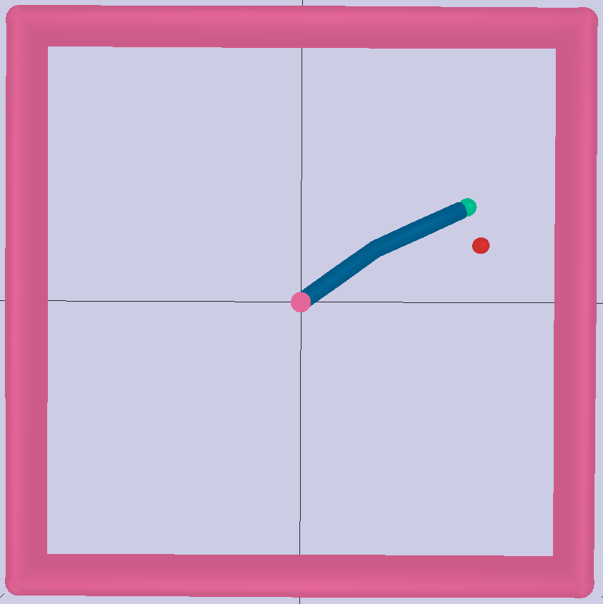
This environment is similar to a continuous action space version of the common grid world problem. In the grid world problem the agent (blue dot) is trying to reach a target location (red dot), shown in the left of Figure 3(a). In this version the agent receives reward for moving closer to its goal ($r=||agent_{pos}-target_{pos}||_{2}$). This problem is chosen because it can be extended to an N-dimensional world very easily, which is helpful as a simple evaluation of scalability as the action-space dimensionality increases. We use a 10D version here [27, 28].

(a) Nav environment and current policy

(b) transition probability error

(c) MBAE direction

Figure 3: The figure (a) left is the current layout of the continuous grid world. The agent is blue and target location for the agent is the red dot and the green boxes are obstacles. In (a) right, the current policy is shown as if the agent was located at each arrow action to give the unit direction of the action. The current value at each state is visualized by the colour of the arrows, red being the highest. In (b) the error of the forward dynamics model is visualized as the distance between the successive state predicted and the actual successive states ($(x+u)-\hat{P}(x,u)$). (c) is the unit length action gradient from MBAE. Only the first two dimensions of the state and action are visualized here.

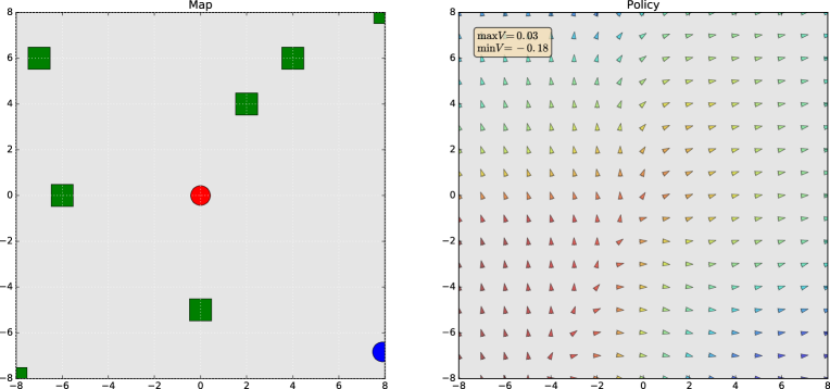
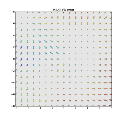
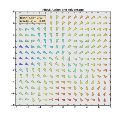
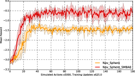
Figure 3 shows a visualization of a number of components used in MBAE. In Figure 5(a) we compare the learning curves of using a standard CACLA learning algorithm and one augmented with MBAE for additional action exploration. The learning curves show a significant improvement in learning speed and policy quality over the standard CACLA algorithm. We also evaluated the impact of pre-training the deterministic transition probability model for MBAE. This pre-training did not provide noticeable improvements.

V-B 2D Biped Imitation

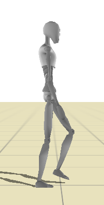
In this environment the agent is rewarded for developing a 2D walking gait. Reward is given for matching an overall desired velocity and for matching a given reference motion. This environment is similar to [29]. The 2D Biped used in the simulation is shown in Figure 4(a).

(a) 2D Biped

(b) 2D Reacher

(c) HalfCheetah

Figure 4: Additional environments MBAE is evaluated on.

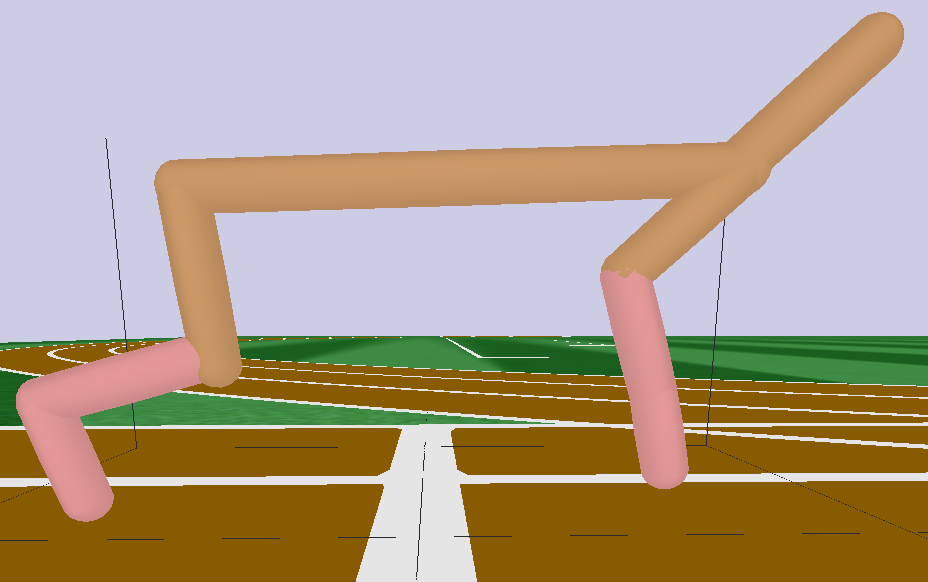
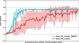
In Figure 5(b), five evaluations are used for the 2D Biped and the mean learning curves are shown. In this case MBAE consistently learns $5$ times faster than the standard CACLA algorithm. We further find that the use of MBAE also leads to improved learning stability and more optimal policies.

V-C Gym and Membrane Robot Examples

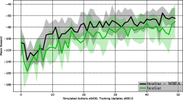
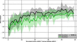
We evaluate MBAE on two environments from openAIGym, 2D Reacher Figure 4(b) and HalfCheetah Figure 4(c). MBAE does not significantly improve the learning speed for the 2D Reacher. However, it results in a higher value policy Figure 5(c). For the HalfCheetah MBAE provides a significant learning improvement Figure 5(d), resulting in a final policy with more than $3$ times the average reward.

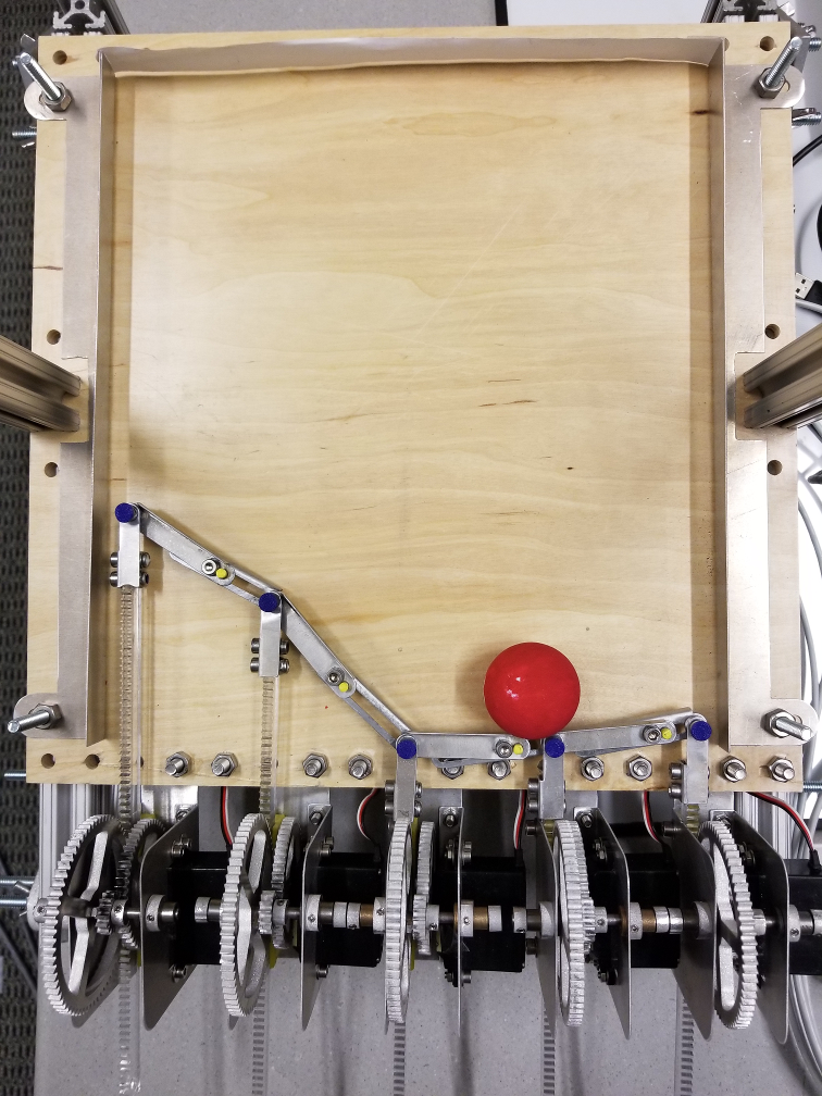
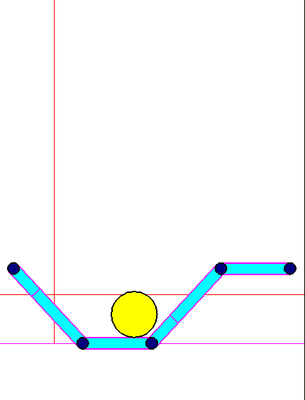
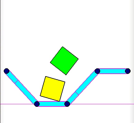
Finally, we evaluate MBAE on a simulation of the juggling Membrane robot shown in Figure 1(a). The under-actuated system with complex dynamics and regular discontinuities due to contacts make this a challenging problem. The results for two tasks that include attempting to stack one box on top of another and a second task to move a ball to a target location are shown in Figure 5(f) and  Figure 5(e). For both these environments the addition of MBAE provides only slight improvements. We believe that due to the complexity of this learning task, it is difficult to learn a good policy for this problem in general. The simulated version of the membrane-stack task is shown in Figure 6(c).

(a) Particle 10D

(b) 2D PD Biped

(c) Reacher 2D

(d) Half-Cheetah

(e) Membrane Target

(f) Membrane Stack

Figure 5: Comparisons of using the CACLA learning method with and without MBAE. These performance curves are the average of $5$ separate simulation with different random seeds.

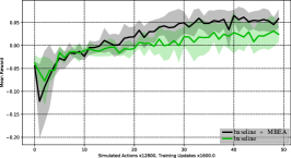
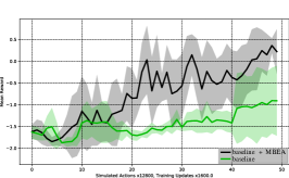
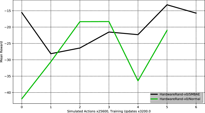
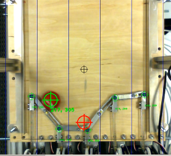
We also asses MBAE on the Membrane robot shown in Figure 1(a). OpenCV is used to track the location of a ball that is affected by the actuation of $5$ servos that cause $5$ pins to move linearly, shown in Figure 6(b). The $5$ pins are connected by passive prismatic joints that form the membrane. The robot begins each new episode by resetting itself which involves tossing the ball up and randomly repositioning the membrane. Please see the accompanying video for details. We transfer the movetotarget policy trained in simulation for use with the Membrane robot. We show the results of training on the robot with and without MBAE for $\sim 3$ hours each in Figure 6(a). Our main objective here is to demonstrate the feasibility of learning on the robot hardware; our current results are only from a single training run for each case. With this caveat in mind, MBAE appears to support improved learning. We believe that this is related to the transition probability model adjusting to the new state distribution of the robot quickly.

(a) Membrane Target

(b) Membrane Camera

(c) Membrane Stack

Figure 6: (a) Comparison of using the MBAE on the physical robot task. (b) is the camera view the robot uses to track its state and (c) is a still frame from the simulated box stacking tasks.

V-D Transition Probability Network Design

We have experimented with many network designs for the transition probability model. We have found that using a DenseNet [30] works well and increases the models accuracy. We use dropout on the input and output layers, as well as the inner layers, to reduce overfitting. This makes the gradients passed through the transition probability model less biased.

VI Discussion

Exploration Action Randomization and Scaling

Initially, when learning begins, the estimated policy gradient is flat, making MBAE actions $\sim 0$. As learning progresses the estimated policy gradient gets sharper leading to actions produced from MBAE with magnitude $>>1$. By using a normalized version of the action gradient, we maintain a reasonably sized explorative action, this is similar to the many methods used to normalize gradients between layers for deep learning [31, 32]. However, with normalized actions, we run the risk of being overly deterministic in action exploration. The addition of positive Gaussian noise to the normalized action length helps compensate for this. Modeling the transition dynamics stochasticity allows us to generate future states from a distribution, further increasing the stochastic nature of the action exploration.

transition probability Model Accuracy

Initially, the models do not need to be significantly accurate. They only have to perform better than random (Gaussian) sampling. We found it important to train the transition probability model while learning. This allows the model to adjust and be most accurate for the changing state distribution observed during training. This makes it more accurate as the policy converges.

MBAE Hyper Parameters

To estimate the policy gradient well and to maintain reasonably accurate value estimates, Gaussian exploration should still be performed. This helps the value function get a better estimate of the current policy performance. From empirical analysis, we have found that sampling actions from MBAE with a probability of $0.25$ has worked well across multiple environments. The learning progress can be more sensitive to the action learning rate $\alpha_{u}$. We found that annealing values between $1.0$ and $0.1$ MBAE assisted learning. The form of normalization that worked the best for MBAE was a form of batchnorm, were we normalize the action standard deviation to be similar to the policy distribution.

One concern could be that MBAE is benefiting mostly from the extra training that is being seen for the value function. We performed an evaluation of this effect by training MBAE without the use of exploratory actions from MBAE. We found no noticeable impact on the learning speed or final policy quality.

VI-A Future Work

It might still be possible to further improve MBAE by pre-training the transition probability model offline. As well, learning a more complex transition probability model similar to what has been done in [16] could improve the accuracy of the MBAE generated actions. It might also be helpful to learn a better model of the reward function using a method similar to [33]. One challenge is the addition of another step size $\alpha$ for how much action gradient should be applied to the policy action, and it can be non-trivial to select this step size.

While we believe that the MBAE is promising, the learning method can suffer from stability issues when the value function is inaccurate, leading to poor gradients. We are currently investigating methods to limit the KL divergence of the policy between updates. These constraints are gaining popularity in recent RL methods [34]. This should reduce the amount the policy shifts from parameter updates, further increasing the stability of learning. The Membrane related tasks are particularly difficult to do well on; even after significant training the policies could still be improved. Lastly, while our focus has been on evaluating the method on many environments, we would also like to evaluate MBAE in the context of additional RL algorithms, such as PPO or Q-Prop, to further assess its benefit.

VII Appendix

VII-A Max Over All Actions, Value Iteration

By using MBAE in an iterative manner, for a single state ($x_{t}$), it is possible to compute the max over all actions. This is a form of value iteration over the space of possible actions. It has been shown that embedding value iteration in the model design can be very beneficial [27] The algorithm to perform this computation is given in Algorithm 3.

Algorithm 3 Action optimization

1:$\hat{u}_{t}\leftarrow\pi(x_{t}|\theta_{\mu})$

2:while not done do

3:      $\hat{u}_{t}\leftarrow\hat{u}_{t}+\textit{GetActionDelta}(\hat{u}_{t})$

4:end while

VII-B More Results

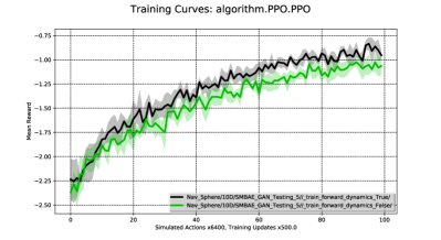
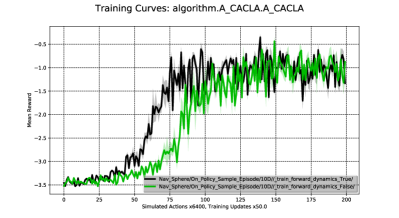
We perform additional evaluation on MBAE. First we use MBAE with the Proximal Policy Optimization (PPO) [35] algorithm in Figure 7(a) to show that the method works with other learning algorithms. We also created a modified version of CACLA that is on-policy to further study the advantage of using MBAE in this setting Figure 7(b).

(a) PPO game

(b) on-policy CACLA game

Figure 7: (a) Result of Applying MBAE to PPO. In (b) we show that an on-policy version of CACLA + MBAE can learn faster than CACLA alone.

References

- [1] I. Osband, D. Russo, Z. Wen, and B. Van Roy, “Deep Exploration via Randomized Value Functions,” ArXiv e-prints, Mar. 2017.
- [2] M. Fortunato, M. Gheshlaghi Azar, B. Piot, J. Menick, I. Osband, A. Graves, V. Mnih, R. Munos, D. Hassabis, O. Pietquin, C. Blundell, and S. Legg, “Noisy Networks for Exploration,” ArXiv e-prints, June 2017.
- [3] M. Plappert, R. Houthooft, P. Dhariwal, S. Sidor, R. Y. Chen, X. Chen, T. Asfour, P. Abbeel, and M. Andrychowicz, “Parameter Space Noise for Exploration,” ArXiv e-prints, June 2017.
- [4] T. P. Lillicrap, J. J. Hunt, A. Pritzel, N. Heess, T. Erez, Y. Tassa, D. Silver, and D. Wierstra, “Continuous control with deep reinforcement learning,” CoRR, vol. abs/1509.02971, 2015. [Online]. Available: http://arxiv.org/abs/1509.02971
- [5] R. S. Sutton and A. G. Barto, Reinforcement learning: An introduction. MIT press Cambridge, 1998, vol. 1, no. 1.
- [6] N. Heess, D. TB, S. Sriram, J. Lemmon, J. Merel, G. Wayne, Y. Tassa, T. Erez, Z. Wang, S. M. A. Eslami, M. Riedmiller, and D. Silver, “Emergence of Locomotion Behaviours in Rich Environments,” ArXiv e-prints, July 2017.
- [7] R. S. Sutton, D. Mcallester, S. Singh, and Y. Mansour, “Policy gradient methods for reinforcement learning with function approximation,” in In Advances in Neural Information Processing Systems 12. MIT Press, 2000, pp. 1057–1063.
- [8] J. Schulman, P. Moritz, S. Levine, M. I. Jordan, and P. Abbeel, “High-dimensional continuous control using generalized advantage estimation,” CoRR, vol. abs/1506.02438, 2015. [Online]. Available: http://arxiv.org/abs/1506.02438
- [9] V. Mnih, A. P. Badia, M. Mirza, A. Graves, T. P. Lillicrap, T. Harley, D. Silver, and K. Kavukcuoglu, “Asynchronous methods for deep reinforcement learning,” CoRR, vol. abs/1602.01783, 2016. [Online]. Available: http://arxiv.org/abs/1602.01783
- [10] V. Mnih, K. Kavukcuoglu, D. Silver, A. A. Rusu, J. Veness, M. G. Bellemare, A. Graves, M. Riedmiller, A. K. Fidjeland, G. Ostrovski, et al., “Human-level control through deep reinforcement learning,” Nature, vol. 518, no. 7540, pp. 529–533, 2015.
- [11] H. Van Hasselt, “Reinforcement learning in continuous state and action spaces,” in Reinforcement Learning. Springer, 2012, pp. 207–251.
- [12] N. Heess, G. Wayne, Y. Tassa, T. P. Lillicrap, M. A. Riedmiller, and D. Silver, “Learning and transfer of modulated locomotor controllers,” CoRR, vol. abs/1610.05182, 2016. [Online]. Available: http://arxiv.org/abs/1610.05182
- [13] X. B. Peng, G. Berseth, K. Yin, and M. Van De Panne, “Deeploco: Dynamic locomotion skills using hierarchical deep reinforcement learning,” ACM Trans. Graph., vol. 36, no. 4, pp. 41:1–41:13, July 2017. [Online]. Available: http://doi.acm.org/10.1145/3072959.3073602
- [14] R. Houthooft, X. Chen, Y. Duan, J. Schulman, F. D. Turck, and P. Abbeel, “Curiosity-driven exploration in deep reinforcement learning via bayesian neural networks,” CoRR, vol. abs/1605.09674, 2016. [Online]. Available: http://arxiv.org/abs/1605.09674
- [15] S. Gu, T. Lillicrap, I. Sutskever, and S. Levine, “Continuous deep q-learning with model-based acceleration,” in Proc. ICML, 2016, pp. 2829–2838.
- [16] N. Mishra, P. Abbeel, and I. Mordatch, “Prediction and control with temporal segment models,” CoRR, vol. abs/1703.04070, 2017. [Online]. Available: http://arxiv.org/abs/1703.04070
- [17] R. S. Sutton, “Dyna, an integrated architecture for learning, planning, and reacting,” ACM SIGART Bulletin, vol. 2, no. 4, pp. 160–163, 1991.
- [18] N. Heess, G. Wayne, D. Silver, T. Lillicrap, T. Erez, and Y. Tassa, “Learning continuous control policies by stochastic value gradients,” in Advances in Neural Information Processing Systems 28, C. Cortes, N. D. Lawrence, D. D. Lee, M. Sugiyama, and R. Garnett, Eds., 2015, pp. 2944–2952.
- [19] A. Nagabandi, G. Kahn, R. S. Fearing, and S. Levine, “Neural Network Dynamics for Model-Based Deep Reinforcement Learning with Model-Free Fine-Tuning,” ArXiv e-prints, Aug. 2017.
- [20] S. Bansal, R. Calandra, S. Levine, and C. Tomlin, “MBMF: Model-Based Priors for Model-Free Reinforcement Learning,” ArXiv e-prints, Sept. 2017.
- [21] I. Goodfellow, J. Pouget-Abadie, M. Mirza, B. Xu, D. Warde-Farley, S. Ozair, A. Courville, and Y. Bengio, “Generative adversarial nets,” in Advances in Neural Information Processing Systems 27, Z. Ghahramani, M. Welling, C. Cortes, N. D. Lawrence, and K. Q. Weinberger, Eds., 2014, pp. 2672–2680.
- [22] P. Isola, J. Zhu, T. Zhou, and A. A. Efros, “Image-to-image translation with conditional adversarial networks,” CoRR, vol. abs/1611.07004, 2016. [Online]. Available: http://arxiv.org/abs/1611.07004
- [23] R. S. Sutton, “Integrated architectures for learning, planning, and reacting based on approximating dynamic programming,” in In Proceedings of the Seventh International Conference on Machine Learning. Morgan Kaufmann, 1990, pp. 216–224.
- [24] D. Silver, G. Lever, N. Heess, T. Degris, D. Wierstra, and M. Riedmiller, “Deterministic policy gradient algorithms,” in Proc. ICML, 2014.
- [25] T. P. Lillicrap, J. J. Hunt, A. Pritzel, N. Heess, T. Erez, Y. Tassa, D. Silver, and D. Wierstra, “Continuous control with deep reinforcement learning,” CoRR, vol. abs/1509.02971, 2015. [Online]. Available: http://arxiv.org/abs/1509.02971
- [26] M. J. Hausknecht and P. Stone, “Deep reinforcement learning in parameterized action space,” CoRR, vol. abs/1511.04143, 2015. [Online]. Available: http://arxiv.org/abs/1511.04143
- [27] A. Tamar, S. Levine, and P. Abbeel, “Value iteration networks,” CoRR, vol. abs/1602.02867, 2016. [Online]. Available: http://arxiv.org/abs/1602.02867
- [28] C. Finn, T. Yu, J. Fu, P. Abbeel, and S. Levine, “Generalizing skills with semi-supervised reinforcement learning,” CoRR, vol. abs/1612.00429, 2016. [Online]. Available: http://arxiv.org/abs/1612.00429
- [29] X. B. Peng and M. van de Panne, “Learning locomotion skills using deeprl: Does the choice of action space matter?” in Proceedings of the ACM SIGGRAPH / Eurographics Symposium on Computer Animation, ser. SCA ’17. New York, NY, USA: ACM, 2017, pp. 12:1–12:13. [Online]. Available: http://doi.acm.org/10.1145/3099564.3099567
- [30] G. Huang, Z. Liu, L. van der Maaten, and K. Q. Weinberger, “Densely connected convolutional networks,” in The IEEE Conference on Computer Vision and Pattern Recognition (CVPR), July 2017.
- [31] J. Lei Ba, J. R. Kiros, and G. E. Hinton, “Layer Normalization,” ArXiv e-prints, July 2016.
- [32] S. Ioffe and C. Szegedy, “Batch normalization: Accelerating deep network training by reducing internal covariate shift,” CoRR, vol. abs/1502.03167, 2015. [Online]. Available: http://arxiv.org/abs/1502.03167
- [33] D. Silver, H. van Hasselt, M. Hessel, T. Schaul, A. Guez, T. Harley, G. Dulac-Arnold, D. Reichert, N. Rabinowitz, A. Barreto, and T. Degris, “The Predictron: End-To-End Learning and Planning,” 2016. [Online]. Available: http://arxiv.org/abs/1612.08810
- [34] J. Schulman, S. Levine, P. Moritz, M. I. Jordan, and P. Abbeel, “Trust region policy optimization,” CoRR, vol. abs/1502.05477, 2015. [Online]. Available: http://arxiv.org/abs/1502.05477
- [35] J. Schulman, F. Wolski, P. Dhariwal, A. Radford, and O. Klimov, “Proximal Policy Optimization Algorithms,” ArXiv e-prints, July 2017.