Discovery of a new fundamental plane dictating galaxy cluster evolution from gravitational lensing

Abstract

In cold dark-matter (CDM) cosmology, objects in the universe have grown under the effect of gravity of dark matter. The intracluster gas in a galaxy cluster was heated when the dark-matter halo formed through gravitational collapse. The potential energy of the gas was converted to thermal energy through this process. However, this process and the thermodynamic history of the gas have not been clearly characterized in connection with with the formation and evolution of the internal structure of dark-matter halos. Here, we show that observational CLASH data of high-mass galaxy clusters lie on a plane in the three-dimensional logarithmic space of their characteristic radius $r_{s}$, mass $M_{s}$, and X-ray temperature $T_{X}$ with a very small orthogonal scatter. The tight correlation indicates that the gas temperature was determined at a specific cluster formation time, which is encoded in $r_{s}$ and $M_{s}$. The plane is tilted with respect to $T_{X}\propto M_{s}/r_{s}$, which is the plane expected in the case of simplified virial equilibrium. We show that this tilt can be explained by a similarity solution, which indicates that clusters are not isolated but continuously growing through matter accretion from their outer environments. Numerical simulations reproduce the observed plane and its angle. This result holds independently of the gas physics implemented in the code, revealing the fundamental origin of this plane.

keywordsgalaxies: clusters: general — cosmology: theory — dark matter — large-scale structure of Universe

1 Introduction

$N$-body numerical simulations show that the density profile of dark-matter halos in galaxy clusters can be well described by the Navarro–Frenk–White (Navarro et al., 1997; NFW, hereafter) density profile: $\rho_{\rm DM}\propto(r/r_{s})^{-1}(1+r/r_{s})^{-2}$, where $r$ is the clustercentric distance and $r_{s}$ is the characteristic or scale radius. We define the mass inside $r_{s}$ as $M_{s}$. Recent higher-resolution simulations have shown that the internal structure of dark-matter halos reflects the growth history of the halos (Wechsler et al., 2002; Zhao et al., 2003; Ludlow et al., 2013; Correa et al., 2015; More et al., 2015). They show that in the early “fast-rate growth” phase, halos grow rapidly through massive matter accumulation. This growth is often associated with phenomena that erase the previous internal structure of the halos, such as major mergers with other halos. In the subsequent “slow-rate growth” phase, halos gradually grow through moderate matter accretion from their surroundings. There are multiple definitions of the formation time of a halo. One example is the time at which the mass of the main progenitor equals the characteristic mass $M_{s}$ of the $z=0$ halo (Ludlow et al., 2013; Correa et al., 2015), and it approximately represents the end of the fast-growth phase and the transitioning toward the slow-growth phase. Only the outskirts of the halos ($r>r_{s}$) gradually grow in the latter phase (Wechsler et al., 2002; Zhao et al., 2003; Ludlow et al., 2013; Correa et al., 2015; More et al., 2015). Thus, dark-matter halos are assembled from the inside out, and the results of the numerical simulations can be interpreted such that the characteristic radius $r_{s}$ and the mass $M_{s}$ preserve a memory of the formation time of the halo (Wechsler et al., 2002; Zhao et al., 2003; Ludlow et al., 2013; Correa et al., 2015). In this “inside-out” scenario of halo formation, halos take a range of characteristic densities ($\rho_{s}\equiv 3M_{s}/(4\pi r_{s}^{3})$); older halos tend to be more concentrated and have larger characteristic densities, which reflects the higher average density of the universe in the past (Navarro et al., 1997; Wechsler et al., 2002; Zhao et al., 2003; Ludlow et al., 2013; Correa et al., 2015; More et al., 2015). This scenario is in contrast with the classical approach in which halos are continuously modified, even by minor mergers, and constantly changing their profiles so that dark-matter halos lose the memory of their epoch of formation (Gunn & Gott, 1972; Press & Schechter, 1974).

If the inside-out halo growth scenario is correct, then we would expect that the formation time not only reflects the structural parameters ($r_{s}$ and $M_{s}$) in the form of the characteristic density ($\rho_{s}$), but also influences the properties of the X-ray intracluster gas. However, its quantitative dependence is not obvious because the gas is collisional matter in contrast with dark matter. The hot gas is expected to be heated mostly via merger shocks produced when smaller halos fall into the halo (Rasia et al., 2011; Kravtsov & Borgani, 2012). However, it is difficult to directly observe the heating process, as the shocks are often located at the outskirts of clusters (Miniati et al., 2000; Ryu et al., 2003), where the gas emission is very faint. We here investigate correlations between the halo parameters ($r_{s},M_{s}$) and the average X-ray gas temperature $T_{X}$ because the temperature is supposedly sensitive to the depth of the potential well and the past heating process (Eke et al., 1998). Since the emissivity of the X-ray gas is proportional to the gas density squared, the average measured temperature of a cluster mainly reflects the temperature in the region ($r\lesssim r_{s}$), where the density is high. While there were previous studies that attempted to investigate correlations among a certain combination of three cluster structural parameters (Schaeffer et al., 1993; Adami et al., 1998; Fujita & Takahara, 1999a; Lanzoni et al., 2004; Ota et al., 2006), they adopted parameters such as the galaxy luminosities that are not directly related to the structure of halos.

In the paper, we assume a spatially flat $\Lambda$CDM cosmology with $\Omega_{\mathrm{m}}=0.27$, $\Omega_{\Lambda}=0.73$, and the Hubble constant of $H_{0}=70$ km s^-1 Mpc^-1 throughout this paper.

2 Observational Data

We study the Cluster Lensing And Supernova survey with Hubble (CLASH) observational dataset that includes 20 massive clusters, most of which are apparently relaxed, X-ray regular systems (Postman et al., 2012; Meneghetti et al., 2014). The range of redshifts is 0.187–0.686, and their median redshift is 0.377 (Umetsu et al., 2016). Lensing constraints on the NFW characteristic radius $r_{s}$ and $M_{s}$ were obtained from a joint analysis of strong-lensing, weak-lensing shear and magnification data of background galaxies (Umetsu et al., 2016). Their analysis is based on 16-band Hubble Space Telescope observations (Zitrin et al., 2015) and wide-field multi-color imaging taken primarily with Suprime-Cam on the Subaru Telescope (Umetsu et al., 2014). The core-excised X-ray temperatures of the clusters were taken from Postman et al. (2012), in which the temperatures are measured for the region of 50–500 kpc from the cluster centers excluding the cool core at the center of the clusters. We chose the outer radius considering the field of view of the Chandra satellite and the completeness of the data. Since most of the X-ray emissions come from $<500$ kpc, the increase of the radius does not affect the results. The cluster data are shown in Table 6.

Figure 1: (a) Points (pin heads) show the distribution of the observed clusters in the space of $(\log(r_{s}/r_{s0}),\log(M_{s}/M_{s0}),\log(T_{\rm X}/T_{\rm X0}))$, where $r_{s0}=570$ kpc, $M_{s0}=3.8\times 10^{14}\>M_{\odot}$, and $T_{\rm X0}=8.2$ keV are the sample geometric averages (log means) of $r_{s}$, $M_{s}$, and $T_{\rm X}$, respectively. The length of a pin shows the distance between the point and the obtained plane. The orange plane is translucent and grayish points are located below the plane. The arrow $P_{1}$ shows the direction on the plane in which the data are most extended, and the arrow $P_{2}$ is perpendicular to $P_{1}$ on the plane. Red bars at the corner of the $\log r_{s}$–$\log M_{s}$ plane and on the $\log T_{\rm X}$ axis are typical $1\sigma$ errors of the data. (b) The cross-section of the plane in (a). The origin is the same as (a) and $P_{3}$ is the plane normal. Large black points are the observations shown in (a). Small red points are the MUSIC simulated clusters projected on the $P_{1}$–$P_{3}$ plane determined for the observed clusters. (c) Same as (a) but error bars for individual clusters are included. The viewing angle is changed so that the relation between the error bars and the plane is easily seen.

3 Fundamental Plane Analysis for the CLASH Sample

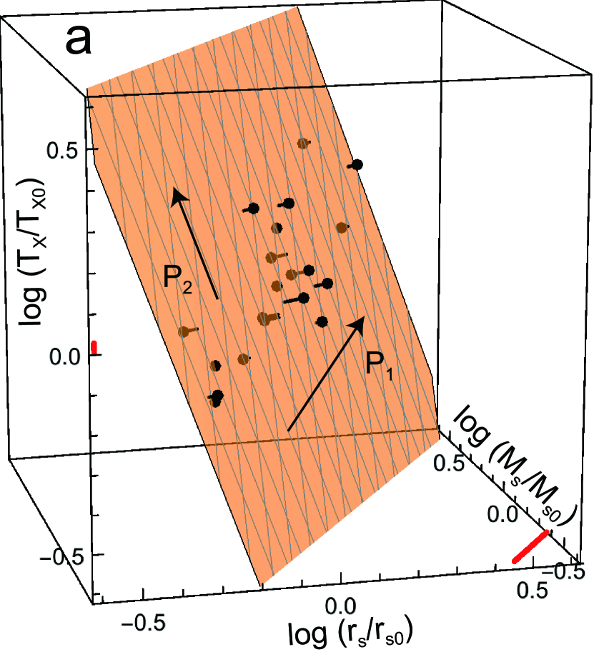
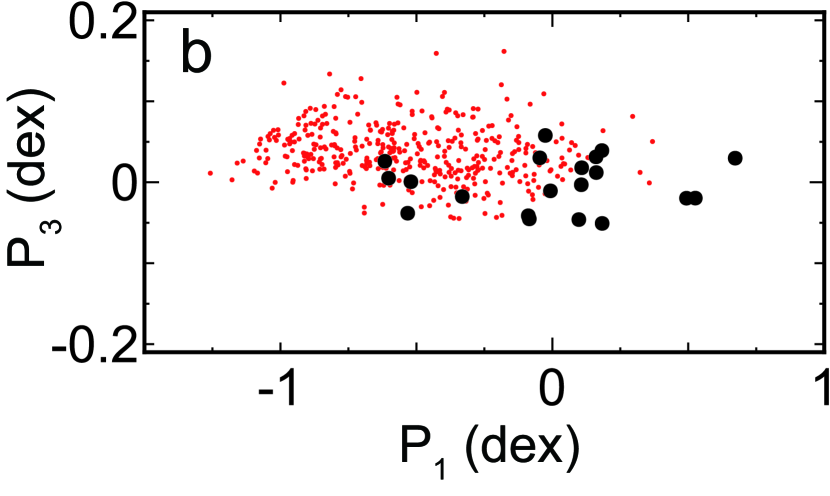
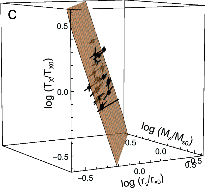
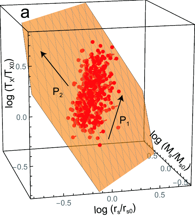
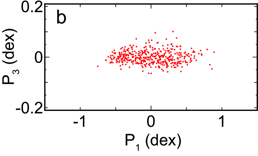
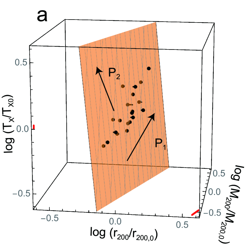
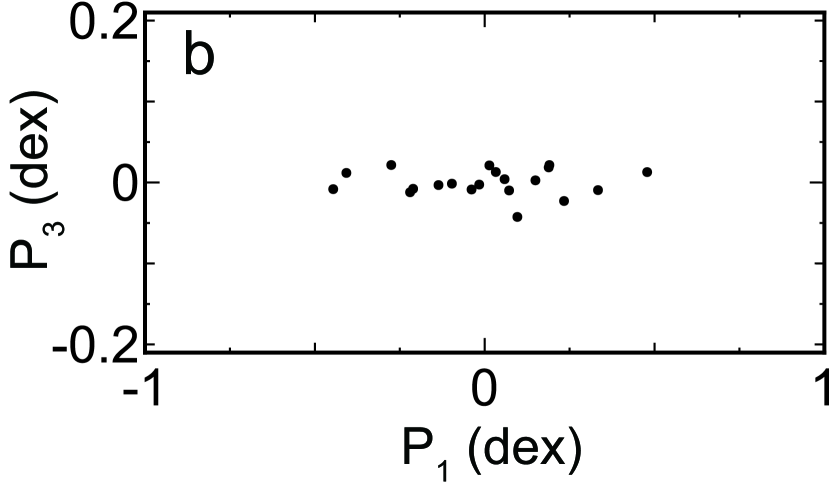
In Figure 1(a), we show the distribution of clusters in the $(\log r_{s},\log M_{s},\log T_{\rm X})$ space. We see that the data points are closely distributed on a plane that we have determined using a principal component analysis (PCA) to minimize deviations of the data points from the plane (see the Appendix). The arrow $P_{1}$ shows the direction on the plane in which the data are most extended, and the arrow $P_{2}$ is perpendicular to $P_{1}$ on the plane. The plane normal is represented by $P_{3}$. The dispersion around the plane or the thickness of the plane is shown in Figure 1(b) and it is only $0.045^{+0.008}_{-0.007}$ dex (all uncertainties are quoted at the $1\>\sigma$ confidence level unless otherwise mentioned). The thickness is comparable to that of the well-known fundamental plane for elliptical galaxies in the space of the surface brightness, the effective radius, and the velocity dispersion ($\sim 0.06$ dex; e.g., La Barbera et al., 2008; Hyde & Bernardi, 2009). In Figure 1(c), we show error bars for individual clusters. In the vertical direction ($T_{\rm X}$), we show the temperature errors in Table 6. In the horizontal direction, however, the errors of $r_{s}$ and $M_{s}$ are highly correlated, and we display them as a single bar. That is, for each cluster, we draw a bar connecting ($r_{s}^{u}$, $M_{s}^{u}$) and ($r_{s}^{l}$, $M_{s}^{l}$), where the superscripts $u$ and $l$ are the upper and the lower limits shown in Table 6, respectively. Note that we have properly accounted for the correlation for each cluster using the joint posterior probability distribution of the NFW parameters (mass and concentration) when we calculate the plane parameters (see the Appendix). Thus, the actual error is not represented by a single bar in a precise sense. The tight planar distribution in Figure 1 indicates that the structure of the dark-matter halos ($r_{s}$ and $M_{s}$) did make a direct influence on the properties of the intracluster gas ($T_{\rm X}$). In the context of the inside-out halo growth scenario, the most natural interpretation of our findings is that the intracluster gas was heated up to around $T_{\rm X}$ in the fast-rate growth phase when the shape of the potential well ($r_{s}$ and $M_{s}$) was established, and that the gas preserves the memory of the cluster formation as is the case of the dark-matter halo structure.

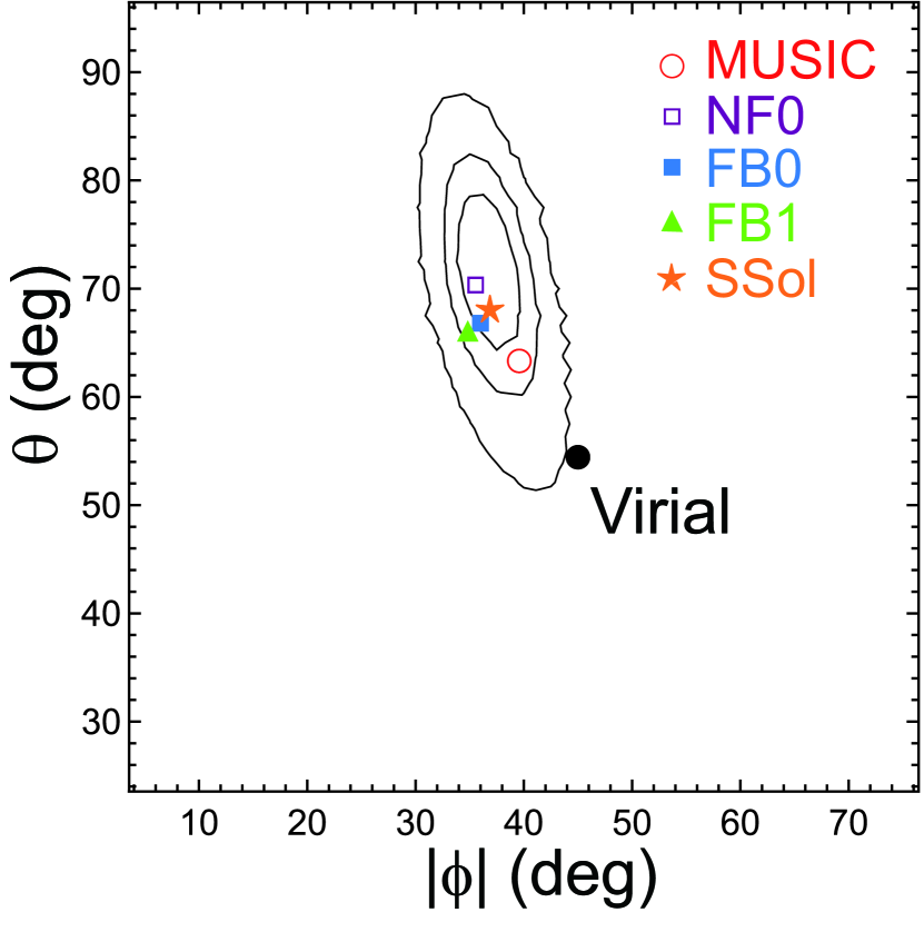
The plane is described by $a\log r_{s}+b\log M_{s}+c\log T_{\rm X}=\mathrm{const.}$, with $a=0.76^{+0.03}_{-0.05}$, $b=-0.56^{+0.02}_{-0.02}$, and $c=0.32^{+0.10}_{-0.09}$. Likelihood contours of the parameters describing the direction of the plane normal, $P_{3}=(a,b,c)$, are shown in Figure 2. The estimation of the errors is described in the Appendix. If the intracluster gas at $r\lesssim r_{s}$ simply preserves its pressure equilibrium state at the cluster formation, the gas temperature should reflect the potential depth of the dark-matter halo at the formation. Thus, one may expect that the gas temperature follows the virial theorem in a narrow sense (“virial expectation”) at that time, $T_{\rm X}\propto M_{s}/r_{s}$, which is one of the main assumptions for the self-similar scaling relations of clusters. The resulting plane, however, is significantly tilted from this virial expectation (Figure 2) and is represented by $T_{\rm X}\propto M_{s}^{-b/c}r_{s}^{-a/c}\propto M_{s}^{1.8\pm 0.5}/r_{s}^{2.3\pm 0.7}$. Our findings show that the temperature $T_{\rm X}$ is more sensitive to the depth of the gravitational potential represented by $M_{s}/r_{s}$ than the canonical virial expectation because $T_{\rm X}\propto M_{s}^{-0.2}r_{s}^{-0.3}(M_{s}/r_{s})^{2.0}$. In other words, clusters with a deeper potential well tend to have higher temperatures $T_{\rm X}$ than the virial expectation, or visa versa.

Figure 2: Direction of the plane normal $P_{3}=(a,b,c)$ in the space of $(\log r_{s},\log M_{s},\log T_{\rm X})$; $\theta$ is the angle between $P_{3}$ and the $\log T_{\rm X}$ axis, and $\phi$ is the azimuthal angle around the $\log T_{\rm X}$ axis, measured anti-clockwise from the $\log r_{s}$ axis, or $\tan\phi=b/a$. Probability contours are shown for the observed clusters at the 68 ($1\>\sigma$), 90, and 99% confidence levels from inside to outside. The contours are elongated in the direction of rotation around $P_{1}$ (Figure 1), to which the direction $P_{3}$ is less constrained. The prediction of the virial expectation ($r_{s}M_{s}^{-1}T_{\rm X}\propto\rm const$) corresponds to $(\phi,\theta)=(-45^{\circ},55^{\circ})$ (black dot), and is rejected at the $>99$% confidence level. Note that for the virial expectation the angle $\theta$ is the one between vectors $(1/\sqrt{3},-1/\sqrt{3},1/\sqrt{3})$ and $(0,0,1)$, which is $\approx 55^{\circ}$. The plane normals derived for simulation samples MUSIC, NF0, FB0, and FB1 are shown by the open red circle, the open purple square, the filled blue square, and the filled green triangle, respectively. All the simulated angles are located inside the 90% contour level and are consistent with the observations at that level. A prediction based on a similarity solution is shown by the orange star (SSol).

Figure 3: Same as Figures 1(a) and (b) but for the MUSIC clusters. The axes are normalized by the average parameters of the sample ($r_{s0}=414$ kpc, $M_{s0}=1.4\times 10^{14}\>M_{\odot}$, and $T_{\rm X0}=3.7$ keV). The plane and the directions $P_{1}$, $P_{2}$, and $P_{3}$ are determined for the MUSIC sample (Table 1).

4 Comparison with Numerical Simulations

Our CLASH sample includes only 20 clusters, and our results may be affected by observational biases. Here, we examine the results of numerical simulations to properly interpret the observations in the context of the CDM cosmology and discuss possible selection bias. First, we analyzed the outputs of MUSIC $N$-body/hydrodynamical simulations (Meneghetti et al., 2014). These are adiabatic; that is, they do not include any nongravitational effects such as feedback from active galactic nuclei (AGNs) or from supernovae (SNe), and there is no radiative cooling.

The details of the simulations for the MUSIC sample are given in Meneghetti et al. (2014). The MUSIC sample is obtained by resimulating halos selected from the MultiDark cosmological simulation (Prada et al., 2012) in order to achieve a higher resolution. The parallel TREEPM+SPH GADGET code (Springel, 2005) is used for the resimulations. The mass resolution for the dark-matter particles is $m_{\rm DM}=9.01\times 10^{8}\>h^{-1}\>M_{\odot}$ and that for the gas particles is $m_{\rm SPH}=1.9\times 10^{8}\>h^{-1}\>M_{\odot}$, where the Hubble constant is written as $H_{0}=100\>h$ km s^-1 Mpc^-1 and $h=0.7$. The gravitational softening is $6\>h^{-1}$ kpc for the both gas and dark-matter particles in the high-resolution regions. We select all of the 402 clusters at $z=0.25$ with $M_{200}>2\times 10^{14}\>h^{-1}\>M_{\odot}$ regardless of dynamical state, where $M_{200}$ is the mass enclosed within a sphere of radius ($r_{200}$) within which the mean overdensity equals 200 times the critical density of the universe. We compute the mass-weighted temperature including the core. The mass-weighted formulation is the most appropriate to evaluate the thermal energy of the X-ray gas to be included in the virial theorem. In addition, we kept the core because these simulations are nonradiative and thus do not present cool-core features. The scale radius $r_{s}$ is obtained by fitting the total density distribution (gas+dark matter) with the NFW profile up to $r_{200}$. The mass $M_{s}$ is then derived as the mass enclosed by a sphere of radius $r_{s}$.

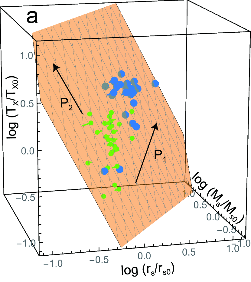
We see that 402 simulated MUSIC clusters at the redshift of $z=0.25$ form a plane in the $(\log r_{s},\log M_{s},\log T_{\rm X})$ space (Figure 3). In Figure 1(b), we project the simulated clusters on the cross-section of the observed plane, showing that the two sets of data are distributed around the same plane ($P_{3}=0$), although the band-like distribution of the MUSIC data is slightly tilted (see Figure 2) while passing through the origin. Many of them are found at smaller $P_{1}$, because the average radius and mass of the MUSIC clusters are smaller than those of the observed clusters by a factor of a few. The plane angle is consistent with the observed one (90% confidence level) and deviates from the virial expectation (Figure 2). The dispersion around the plane for the simulated clusters is $0.025$ dex and is even smaller than the observed one ($0.045^{+0.008}_{-0.007}$ dex; Table 1). Since unrelaxed clusters tend to have disturbed internal structure, they are expected to increase the dispersion. However, even when we choose the 20% most unrelaxed (UR) clusters in the sample, it is only 0.033. Therefore, the slightly larger observed thickness of the plane is unlikely ascribable to the dynamical state of the systems. The direction of the plane for the UR clusters is also not much different from that of the full sample (Table 1). Although our CLASH clusters are relatively massive and relaxed, these results of the numerical simulations show that the selection bias should not significantly affect the derived plane parameters.

To study the evolution in detail, we analyzed another set of simulation data (Rasia et al., 2015). Each of the samples named FB0 and NF0 consists of 29 massive clusters at $z=0$, and contain both relaxed and unrelaxed ones. FB0 includes nongravitational effects and NF0 does not. The details of the simulations for samples FB0, FB1, and NB0 are given in Rasia et al. (2015) and Planelles et al. (2017). They are also carried out with the GADGET code (Springel, 2005) but including an updated SPH scheme (Beck et al., 2016). The simulations consist in 29 Lagrangian regions around massive clusters with $M_{\rm 200}\sim 1$–$30\times 10^{14}\>h^{-1}\>M_{\odot}$ at $z=0$. The simulations FB0 and FB1 include phenomena such as heating by AGNs and SNe in addition to radiative cooling, while NF0 is from nonradiative runs. Samples FB0 and NF0 consist of the clusters at $z=0$, while sample FB1 refers to the runs at $z=1$. The mass resolution for the dark-matter particles is $m_{\rm DM}=8.3\times 10^{8}\>h^{-1}\>M_{\odot}$ and that for the initial gas particles is $m_{\rm SPH}=1.5\times 10^{8}\>h^{-1}\>M_{\odot}$. The gravitational softening is $3.75\>h^{-1}$ kpc for both the gas and dark-matter particles in the high-resolution regions (Biffi et al., 2017). We derive $r_{s}$ and $M_{s}$ for the clusters in the FB0, FB1, and NB0 samples using the same method exploited for the MUSIC simulations. Since this sample, contrary to the previous sample, is built on radiative simulations we do exclude the core. As we did for the observed CLASH sample, the temperatures are obtained in the region between 50 and 500 kpc from the cluster centers. Although we use the mass-weighted temperature in the following discussion, we have confirmed that the results such as the plane angle and thickness are not significantly affected by the choice of the temperature weighting (e.g. spectroscopic-like temperature; Mazzotta et al. 2004) or the choice of the metric radius for temperature measurements ($>500$ kpc).

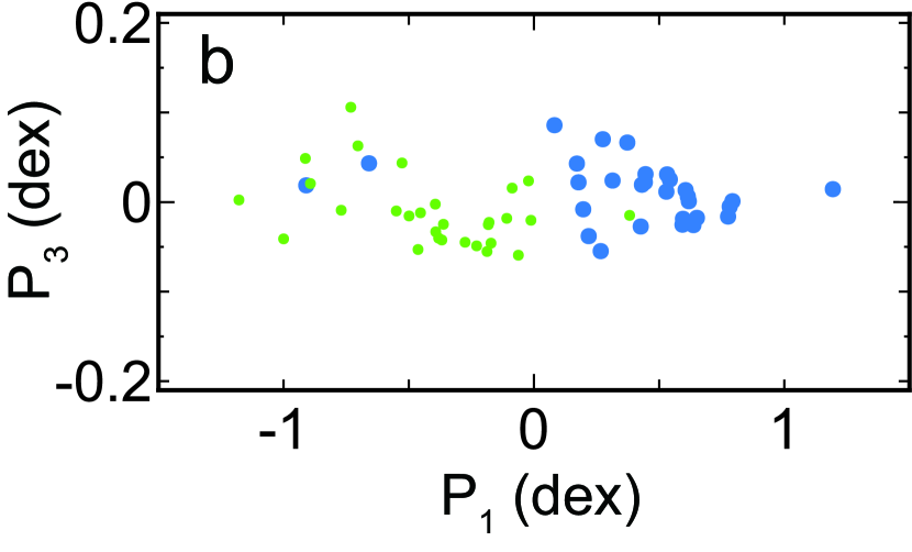
We find that each sample forms a plane whose angle is consistent with the observed one (Figure 2). The plane angles for FB0 and NF0 are almost the same, which means that the result is independent of the gas physics. The lack of dependence means that radiative cooling and SNe and AGN feedback counterbalance one another with the effect of not drastically changing the X-ray gas profile on a scale of $r_{s}$. Thus, even if our CLASH clusters are affected by some selection bias originating from gas physics (e.g. difference of AGN activities), the bias does not have a significant impact on the plane parameters. The thickness of the plane is, however, increased by the nongravitational effects. In fact, the dispersion around the plane for FB0 is $0.031$ dex, which is larger than that for NF0 ($0.023$ dex), but is still smaller than the observed one even if the observational errors are considered (Table 1). In Figure 2, we also show the plane angle for clusters in the same simulation as FB0 but at $z=1$ (sample FB1). Most of the clusters (25/29) are the progenitors of those in FB0. While more clusters should be in the fast-rate growth phase at $z=1$, the plane angle is not much different from that at $z=0$ (FB0). We find that the clusters in the samples FB0 and FB1 are virtually on the same plane (Figure 4); though, FB1 clusters tend to have smaller physical radii and masses. This indicates that the redshifts of the clusters are unlikely to impact the plane parameters. The dispersion around the common plane is $0.037$ dex (FB0+FB1 in Table 1). This indicates that the clusters evolve on this unique plane along the direction of $P_{1}$, and that the evolution of cluster halo structure and the thermodynamic history of intracluster gas are strictly regulated by the plane.

In general, current numerical simulations are realistically reproducing the observed scaling relations including their slopes (Truong et al., 2018). Any possible small discrepancy of the normalizations does not significantly affect the plane angle and the cluster evolution along the plane.

Figure 4: Same as Figures 1(a) and (b) but for the simulated clusters. Large blue and small green points show the simulation samples FB0 ($z=0$) and FB1 ($z=1$), respectively. The axes are normalized by the average parameters of the combined sample (FB0+FB1; $r_{s0}=388$ kpc, $M_{s0}=1.4\times 10^{14}\>M_{\odot}$, and $T_{\rm X0}=4.8$ keV). The plane and the directions $P_{1}$, $P_{2}$, and $P_{3}$ are determined for the combined sample (Table 1).

Figure 5: (a) Projection of the MUSIC data points in Figure 3(a) on the $\log r_{s}$–$\log M_{s}$ plane. The normalizations of the axes are the same as those in Figure 3. Each dashed line satisfies $\rho_{s}=\rm const$ and the value of the constant increases in the direction of the thin dotted arrow. The thick solid arrow represents a line $r_{s}\propto M_{s}^{1/2}$, and the value $M_{s}r_{s}^{1/2}$ increases in the direction. (b) $T_{\rm X}$ is plotted against $M_{s}r_{s}^{1/2}$. (c) $T_{\rm X}$ is plotted against $\rho_{s}$. Evolution of a typical cluster belonging to FB0+FB1 is shown in the solid line. Prominent features are marked by the labels A, B, …, F. The cluster and the labels are the same as those in Figure 6. The green arrow shows the projected direction of $P_{1}$ for the MUSIC data.

Figure 6: (a) Evolution of $r_{s}$ (black solid), $M_{s}$ (red dotted), and $T_{\rm X}$ (blue dashed) of a typical cluster in the sample FB0+FB1. The time $t$ is the cosmological one. Prominent features are marked by the labels A, B, …, F. The area of the filled circles at the bottom is proportional to the reduced $\chi^{2}$ of the fit to the NFW profile. (b) Evolution of the cluster in the plane coordinate that is the same as that in Figure 4. The labels A, B, …, F correspond to those in (a). Note that scales of the axes $P_{1}$, $P_{2}$, and $P_{3}$ are different.

5 Discussion

5.1 The plane angle predicted by a similarity solution and cluster evolution

In this subsection, we attempt to explain the origin of the peculiar plane angle we found using an analytic solution. Bertschinger (1985) constructed a one-dimensional similarity solution for secondary infall and accretion onto an initially overdense perturbation in an Einstein-de Sitter ($\Omega_{0}=1$) universe. For this solution, an object continues to grow, and the matter density $\rho$, pressure $p$ at the radius $r$, and mass $m$ inside $r$ at the cosmological time $t$ can be expressed by nondimensional functions ($D$, $P$, and $M$):

$$\rho(r,t) = \rho_{\rm H}D(\lambda)\>,$$

$$p(r,t) = \rho_{\rm H}(r_{\rm ta}/t)^{2}P(\lambda)\>,$$ (1)

$$m(r,t) = (4\pi/3)\rho_{\rm H}r_{\rm ta}^{3}M(\lambda)\>,$$

where $r_{\rm ta}(t)$ is the maximum radius that a mass shell reaches (the turnaround radius), $\rho_{\rm H}\propto t^{-2}$ is the density of the background universe, and $\lambda=r/r_{\rm ta}$ is the nondimensional radius. The turnaround radius is represented by $r_{\rm ta}=A_{\rm ita}t^{8/9}$, where $A_{\rm ita}$ is the coefficient that depends on the overdense perturbation (Bertschinger, 1985). The solution has an entropy integral,

$$P(\lambda)D(\lambda)^{-\gamma}M(\lambda)^{10/3-3\gamma}={\rm const}\>,$$ (2)

where $\gamma=5/3$ is the adiabatic index. This relation holds even for a system with a mixture of gas and dark matter (Bertschinger, 1985). From equations (5.1) and (2), we have $p\rho^{-5/3}m^{-5/3}\propto A_{\rm ita}^{-3}$, which does not depend on $t$. The coefficient can be written as $A_{\rm ita}=r_{\rm ita}/t_{\rm ita}^{8/9}$, where $r_{\rm ita}$ and $t_{\rm ita}$ are the turnaround radius and time of the overdense perturbation, respectively. Note that $t_{\rm ita}$ is much earlier than “the formation of a cluster” discussed in this study. Assuming that the evolution of the overdense perturbation follows a theory of a spherical collapse, they are represented by

$$r_{\rm ita}\propto m_{\rm ita}^{(n+5)/6},\hskip 42.67912ptt_{\rm ita}\propto m_{\rm ita}^{(n+3)/4}\>,$$ (3)

where $m_{\rm ita}$ is the mass scale of the perturbation and $n$ is the local slope of the primordial matter power spectrum (Kaiser, 1986; Peebles, 1993), which is $n\sim-2$ at cluster scales (Eisenstein & Hu, 1998; Diemer & Kravtsov, 2015). Thus, we obtain $p\rho^{-5/3}m^{-5/3}\propto m_{\rm ita}^{-5/6}$. Assuming that $p\propto\rho T_{\rm X}$ and $\rho\propto M_{s}/r_{s}^{3}$ at $r\sim r_{s}$, the relation is $r_{s}^{2}M_{s}^{-7/3}T_{\rm X}\propto m_{\rm ita}^{-5/6}$. Here, we speculate that the structure of the NFW profile at $r\lesssim r_{s}$ reflects the overdense perturbation that initially collapsed in the similarity solution by Bertschinger (1985). In other words, the fast-rate growth of a dark-matter halo is related to the initial collapse. In fact, Correa et al. (2015) demonstrated that the characteristic density $\rho_{s}$ of the NFW profile is proportional to the critical density of the background universe $\rho_{c}$ at the time when the dark-matter halo transits from the fast-rate to the slow-rate growth phase (i.e. the halo formation time). On the other hand, since the initial collapse can be described as a simple spherical collapse of an overdense region, the typical density of the collapsed object is also proportional to $\rho_{c}$ at the collapse time (Bertschinger, 1985). This indicates that both the inner structure of the NFW profile and the overdense perturbation in the similarity solution follow the same evolution and scaling relation. Thus, we assume $M_{s}\propto m_{\rm ita}$ and $r_{s}\propto r_{\rm ita}$, which leads to

$$r_{s}^{2}M_{s}^{-3/2}T_{\rm X}={\rm const}\>.$$ (4)

The angle of this plane is shown in Figure 2 (SSol) and it is consistent with the observations. The essential point of the similarity solution is that clusters are not isolated but continuously growing through matter accretion from their outer environments. Therefore, additional contributions, such as the flux of inertia at the cluster surface, should be included in the virial theorem for the complete description of the dynamical state (Bertschinger, 1985). In the $\Lambda$CDM model (Peebles, 1993), the cosmological constant becomes non-negligible at $z\lesssim((1-\Omega_{m})/\Omega_{m})^{1/3}-1\sim 0.39$, which is close to the median redshift of our observational sample (Table 1). Thus, about half of the sample may be affected by the cosmological constant. However, although the density profiles of these objects may become steeper in the outskirts (Bertschinger, 1985), the effect is not serious because we are interested in the inner region ($r\lesssim r_{s}$).

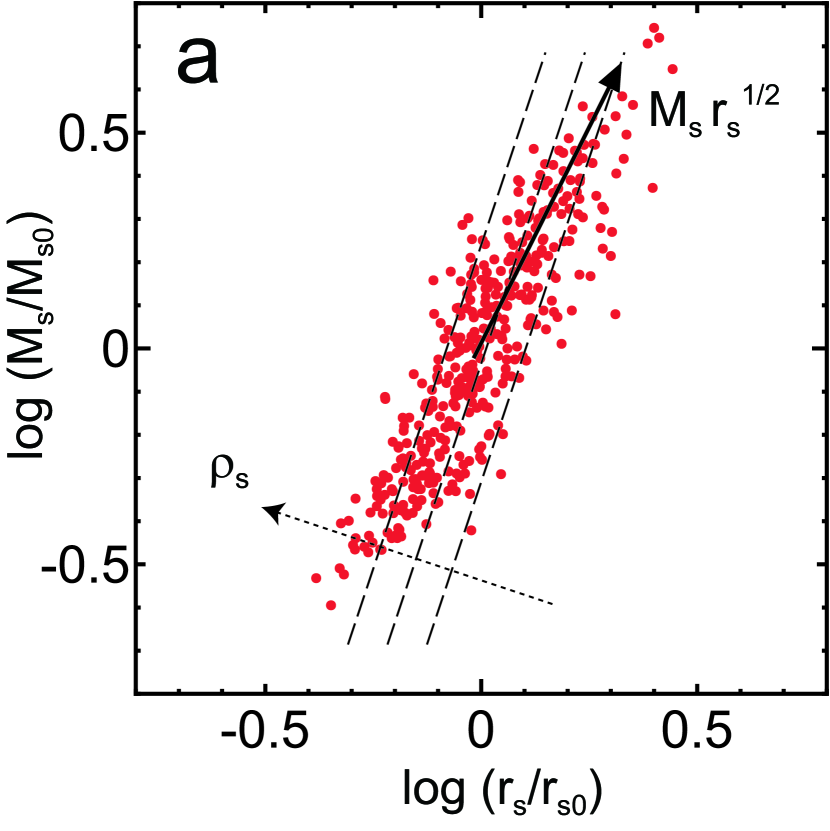
This simple model may also explain the vector $P_{1}$. Since we assumed $r_{s}\propto r_{\rm ita}$ and $M_{s}\propto m_{\rm ita}$, we obtain $r_{s}\propto M_{s}^{1/2}$ from equation (3). The direction of the line $r_{s}\propto M_{s}^{1/2}$ on the $\log r_{s}$–$\log M_{s}$ plane is almost the same as that of $P_{1}$ projected on the $\log r_{s}$–$\log M_{s}$ plane, especially for $P_{1}$ for the simulation samples (Table 1). Figure 5(a) shows that the MUSIC data points are actually distributed along the line $r_{s}\propto M_{s}^{1/2}$ (thick solid arrow) on the $\log r_{s}$–$\log M_{s}$ plane. This means that the cluster’s elongated distributions along $P_{1}$ (Figures 3 and 4) reflect the evolution of the typical overdense perturbation along $r_{\rm ita}\propto m_{\rm ita}^{1/2}$, which can also be interpreted as the evolution of clusters during the fast-rate growth phase. The direction of $P_{1}$ for the observational sample (first line of Table 1) is slightly different from those for the simulations. This may be because the observational sample is biased toward high temperature clusters.

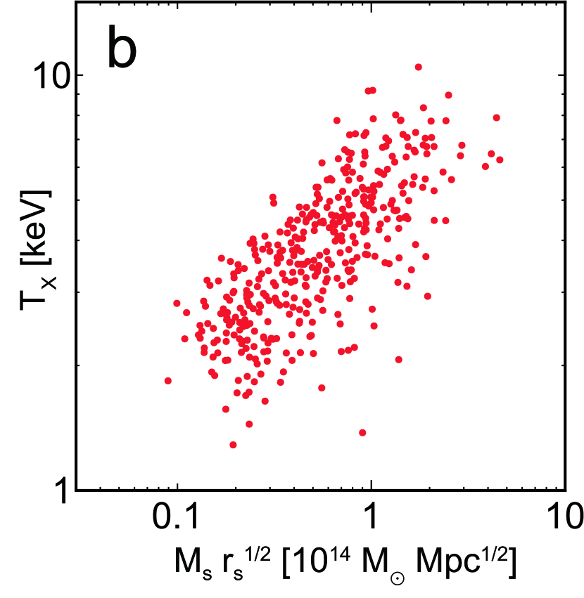
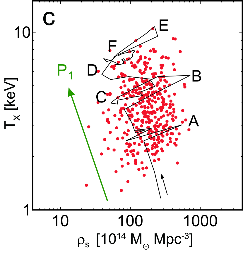
Cluster formation time is associated with the characteristic density (e.g. Fujita & Takahara, 1999b; Ludlow et al., 2013; Correa et al., 2015). The dashed lines in Figure 5(a) are isochrones or $\rho_{s}=\rm const$. The MUSIC data points are widely distributed along each isochrone, which reflects a variety of cluster masses for a given formation time. In other words, it reflects a variety of peak densities of initial density fluctuations of the universe. Individual clusters evolve approximately in the direction of $P_{1}$ (Figures 3 and 4), or in the direction to which $M_{s}r_{s}^{1/2}$ increases (Figure 5(a)), that is, along the line $r_{s}\propto M_{s}^{1/2}$ ($r_{s}\propto M_{s}^{1/1.65}$ in a detailed study; Zhao et al. 2009). Figure 5(b) shows that $M_{s}r_{s}^{1/2}$ and $T_{\rm X}$ are correlated, which reflects that $T_{\rm X}$ evolves according to the structure evolution of dark halos, although the projection of the band-like distribution of clusters in Figure 3(a) onto the $M_{s}r_{s}^{1/2}$–$T_{\rm X}$ plane disperses the relation. In Figure 5(a), clusters become denser (having larger $\rho_{s}$) or older in the direction of the thin dotted arrow. In Figure 5(c), the correlation between $\rho_{s}$ and $T_{\rm X}$ is not clear, because a possible correlation is obscured by the projection of clusters with various masses along the dashed lines in Figure 5(a) (see also Figure 3(a)). However, each cluster moves mainly along the direction of $P_{1}$, which shows that the cluster temperature increases as the density $\rho_{s}$ decreases, although major mergers (A, B, and E in Figure 5(c)) derail the cluster significantly from the evolution along $P_{1}$. We emphasize that the MUSIC data distribution on the plane does not follow a single line but has a finite spread, and $M_{s}$ has a distribution for a given formation time. In general, the correlation between some two parameters of clusters is not necessarily represented by a line but is often represented by a broad band (Figure 5). This is because the mass scale of the initial density fluctuation of the universe has a distribution for a given peak height (e.g. Barkana & Loeb, 2001). Since the peak height also has its own distribution, these result in a two-dimensional band-like distribution of clusters. In general, clusters move along the band on the plane in the direction of $P_{1}$ (see also the next subsection).

Figure 7: Same as Figures 1(a) and (b), but in the space of $(\log(r_{200}/r_{200,0}),\log(M_{200}/M_{200,0}),\log(T_{\rm X}/T_{\rm X0}))$, where $r_{200,0}=2040$ kpc, $M_{200,0}=1.4\times 10^{15}\>M_{\odot}$, and $T_{\rm X0}=8.2$ keV are the sample averages of $r_{200}$, $M_{200}$, and $T_{\rm X}$, respectively.

5.2 Stability of the plane against mergers

The similarity of clusters is generally good because most of them are well represented by the NFW profile. The thinness of the plane reflects the excellent similarity because cluster structure is well described by the similarity solution discussed in Section 5.1. However, clusters occasionally experience mergers that might break the similarity.

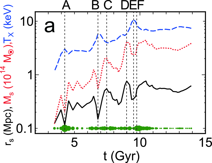
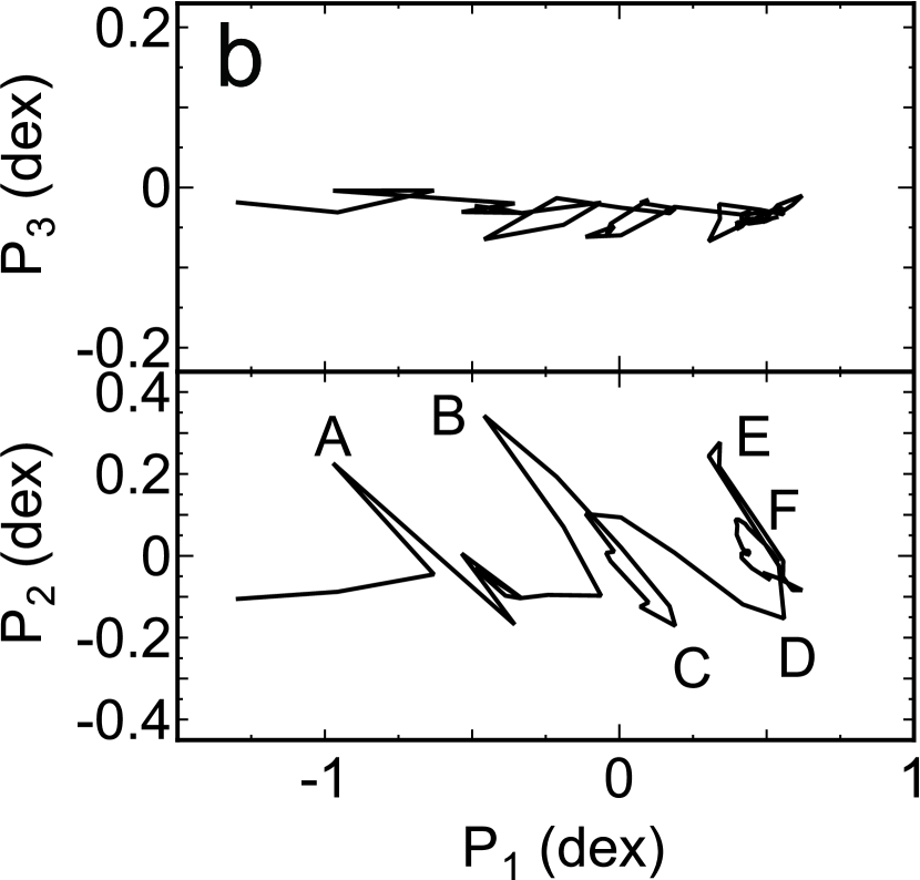
In Figure 6(a), we follow the evolution of a cluster that undergoes three major mergers in the sample FB0+FB1. This cluster experiences mergers around the times indicated by A, B, and E. While $M_{s}$ tends to correlate with $r_{s}$, the temperature $T_{\rm X}$ tends to inversely correlate with $r_{s}$. This can be explained as follows. When a large substructure is merging with a cluster, it does not dissolve immediately when it touches the viral radius of the cluster. The 3D cluster gas density profiles will, therefore, include the gas of the substructure as it moves within the cluster external atmosphere toward the inner regions. Very large substructures can even reach the center and cross it. This is the main origin of changing $r_{s}$ and $M_{s}$: when the substructure is in the outskirts, the profile is flatter and thus $r_{s}$ and $M_{s}$ are larger (less concentrated cluster), while when the substructure is closer to the center, the object appears more concentrated, i.e. with smaller $r_{s}$ and $M_{s}$. On the other hand, $T_{\rm X}$ increases for a moment, after the shock has time to propagate throughout a large region of the cluster.

Thanks to the behavior of the three parameters $r_{s}$, $M_{s}$, and $T_{\rm X}$, the cluster does not substantially deviate from the plane ($P_{3}=0$) even during a merger (Figure 6(b)), which contributes to the thinness of the plane. Figure 6 also shows that after the end of the last major merger indicated by the letter F, the three parameters do not change much and the cluster remains in almost the same position on the plane. This indicates that the current cluster structure is determined at the last major merger.

5.3 Cluster distribution in the space of $(\log r_{200},\log M_{200},\log T_{\rm X})$.

Contrary to the inside-out scenario, dark-matter halos possess only a common global density that is related to the virial overdensity in the classical picture of cluster formation (Gunn & Gott, 1972; Press & Schechter, 1974; Lacey & Cole, 1993). A representative density is $\rho_{200}$, which is 200 times the critical density of the universe at the cluster redshift. Individual halos can thus be characterized by $M_{200}$, the mass enclosed within a sphere of radius $r_{200}$ within which the mean overdensity equals $\rho_{200}$. The mass $M_{200}$ is often regarded as the total mass of a cluster. The values of $r_{200}$ and $M_{200}$ for our observed clusters are shown in Table 6.

As an alternative parameter combination, we check the cluster distribution in the space of $(\log r_{200},\log M_{200}$, $\log T_{\rm X})$. In Figure 7(a), the data points are distributed on a plane almost vertical to the $\log r_{200}$–$\log M_{200}$ plane, which reflects the obvious relation of $M_{200}=4\pi\rho_{200}r_{200}^{3}/3\propto r_{200}^{3}$ regardless of $T_{\rm X}$. The redshift dependence of $\rho_{200}$ is small because the majority of the clusters in our sample are distributed in a relatively narrow range at low-intermediate redshifts, although the small redshift dependence slightly slants the the plane. The dispersion in the direction of the plane normal ($P_{3}$) is small (Figure 7(b); $0.016^{+0.001}_{-0.001}$ dex). A weak correlation ($P_{1}$), in which clusters with a larger $M_{200}$ tend to have a larger $T_{\rm X}$, is seen on the plane, but the dispersion ($P_{2}$) is relatively large (Figure 7(a); $0.099^{+0.011}_{-0.011}$ dex). Although this correlation $P_{1}$ has been studied as a mass–temperature relation (e.g. Sun et al., 2009; Connor et al., 2014), the large dispersion suggests that it is not a primary relation, and that the combination of parameters ($r_{s},M_{s},T_{\rm X}$) rather than $(r_{200},M_{200},T_{\rm X})$ is appropriate for studying the connection between the X-ray gas and the dark halo structure and the interplay between gas heating and gravitational collapse in detail. The well-known large scatter of the concentration ($c_{200}\equiv r_{200}/r_{s}$)–mass ($M_{200}$) relation (e.g. Bullock et al., 2001) may be because $r_{s}$ has less to do with $r_{200}$ and $M_{200}$.

6 Conclusions

In this study, we showed that observational data of high-mass galaxy clusters form a plane in the three-dimensional logarithmic space of their characteristic radius $r_{s}$, mass $M_{s}$, and X-ray temperature $T_{\rm X}$ with a very small orthogonal scatter. Since the evolution history of a cluster is encoded in $r_{s}$ and $M_{s}$, the tight correlation suggests that the gas temperature was determined at a specific cluster formation time. We also found that the plane is tilted with respect to $T_{\rm X}\propto M_{s}/r_{s}$, which is the plane expected in the case of simplified virial equilibrium. This strange plane angle can be explained by a similarity solution, which indicates that clusters are not isolated but continuously growing through matter accretion from their outer environments. In other words, the effects of the growth must be considered when the internal structure of clusters is discussed. We have shown that numerical simulations reproduce the observed plane and its angle, regardless of the gas physics implemented in the code. The simulations show that clusters evolve along the plane and they do not deviate much from the plane even during major mergers, which contributes to the overall thinness of the plane.

Further work is needed to understand the relation between the similarity solution and the formation of the NFW halo structure (Salvador-Solé et al., 1998; Williams et al., 2004). Large-scale high-resolution numerical simulations from high to low redshifts would be useful to study these topics. It would also be interesting to extend the observational sample to objects other than massive clusters in the nearby universe. Those objects include clusters at higher redshifts and less massive systems, such as galaxy groups and elliptical galaxies that present a break from the cluster self-similarity behavior (Ponman et al., 1999). It would also be interesting to study relationships between the cluster plane and galactic-scale ones (e.g. Goulding et al. 2016). Galaxy clusters have been used to constrain cosmological parameters, such as the amount of matter and dark energy, and to investigate the growth of large-scale structure. In particular, the evolution of the abundance of rare massive clusters above a given mass threshold is highly sensitive to the expansion history and the growth rate of mass density fluctuations (e.g. Vikhlinin et al., 2009). Thanks to the thinness of the plane we discovered, precise determinations of the fundamental plane can be used to calibrate cluster mass–observable relations, a key ingredient of the cluster cosmology (Fujita et al., 2018).

Table 2: Cluster data

Cluster	$z$	$r_{s}$	$r_{200}$	$M_{s}$	$M_{200}$	$T_{\rm X}$
		(kpc)	(kpc)	($10^{14}\>M_{\odot}$)	($10^{14}\>M_{\odot}$)	(keV)
Abell 383	0.187	$304^{+159}_{-97}$	$1800^{+209}_{-189}$	$1.4^{+1.0}_{-0.5}$	$7.9^{+3.1}_{-2.2}$	$6.5\pm 0.24$
Abell 209	0.206	$834^{+243}_{-192}$	$2238^{+161}_{-172}$	$5.2^{+2.2}_{-1.6}$	$15.4^{+3.6}_{-3.3}$	$7.3\pm 0.54$
Abell 2261	0.224	$682^{+232}_{-170}$	$2542^{+192}_{-188}$	$5.8^{+2.7}_{-1.8}$	$22.9^{+5.6}_{-4.7}$	$7.6\pm 0.30$
RX J2129.7+0005	0.234	$294^{+133}_{-89}$	$1626^{+163}_{-154}$	$1.1^{+0.7}_{-0.4}$	$6.1^{+2.0}_{-1.6}$	$5.8\pm 0.40$
Abell 611	0.288	$560^{+250}_{-172}$	$2189^{+204}_{-208}$	$3.8^{+2.3}_{-1.5}$	$15.6^{+4.8}_{-4.0}$	$7.9\pm 0.35$
MS 2137-2353	0.313	$784^{+557}_{-357}$	$2064^{+261}_{-286}$	$4.7^{+5.2}_{-2.6}$	$13.4^{+5.8}_{-4.9}$	$5.9\pm 0.30$
RX J2248.7-4431	0.348	$643^{+422}_{-246}$	$2267^{+282}_{-261}$	$4.9^{+4.8}_{-2.3}$	$18.5^{+7.8}_{-5.7}$	$12.4\pm 0.60$
MACS J1115.9+0129	0.352	$738^{+249}_{-196}$	$2186^{+161}_{-174}$	$5.1^{+2.4}_{-1.7}$	$16.6^{+4.0}_{-3.7}$	$8.0\pm 0.40$
MACS J1931.8-2635	0.352	$501^{+441}_{-221}$	$2114^{+355}_{-311}$	$3.5^{+4.6}_{-1.8}$	$15.0^{+8.9}_{-5.7}$	$6.7\pm 0.40$
RX J1532.9+3021	0.363	$293^{+433}_{-114}$	$1544^{+191}_{-210}$	$1.2^{+1.6}_{-0.5}$	$5.9^{+2.5}_{-2.1}$	$5.5\pm 0.40$
MACS J1720.3+3536	0.391	$505^{+248}_{-162}$	$2055^{+204}_{-204}$	$3.4^{+2.3}_{-1.4}$	$14.4^{+4.7}_{-3.9}$	$6.6\pm 0.40$
MACS J0416.1-2403	0.396	$642^{+201}_{-156}$	$1860^{+146}_{-154}$	$3.4^{+1.5}_{-1.1}$	$10.7^{+2.7}_{-2.4}$	$7.5\pm 0.80$
MACS J0429.6-0253	0.399	$394^{+238}_{-143}$	$1792^{+225}_{-208}$	$2.1^{+1.8}_{-0.9}$	$9.6^{+4.1}_{-3.0}$	$6.0\pm 0.44$
MACS J1206.2-0847	0.440	$587^{+248}_{-176}$	$2181^{+165}_{-178}$	$4.6^{+2.4}_{-1.7}$	$18.1^{+4.4}_{-4.1}$	$10.8\pm 0.60$
MACS J0329.7-0211	0.450	$254^{+95}_{-63}$	$1697^{+129}_{-127}$	$1.4^{+0.6}_{-0.4}$	$8.6^{+2.1}_{-1.8}$	$8.0\pm 0.50$
RX J1347.5-1145	0.451	$840^{+339}_{-239}$	$2684^{+226}_{-230}$	$9.8^{+5.6}_{-3.6}$	$34.2^{+9.4}_{-8.1}$	$15.5\pm 0.60$
MACS J1149.5+2223	0.544	$1108^{+404}_{-291}$	$2334^{+169}_{-178}$	$10.8^{+5.4}_{-3.7}$	$25.0^{+5.8}_{-5.3}$	$8.7\pm 0.90$
MACS J0717.5+3745	0.548	$1300^{+347}_{-271}$	$2387^{+154}_{-165}$	$13.2^{+5.3}_{-3.9}$	$26.8^{+5.6}_{-5.2}$	$12.5\pm 0.70$
MACS J0647.7+7015	0.584	$468^{+254}_{-160}$	$1884^{+189}_{-192}$	$3.3^{+2.3}_{-1.3}$	$13.7^{+4.6}_{-3.8}$	$13.3\pm 1.80$
MACS J0744.9+3927	0.686	$574^{+269}_{-192}$	$1982^{+179}_{-185}$	$4.9^{+3.1}_{-2.0}$	$17.9^{+5.3}_{-4.6}$	$8.9\pm 0.80$

Table 1: Cluster Samples

	Observation	Simulations
		MUSIC	NF0	FB0	FB1	FB0+FB1
Nongravitational effects	$\cdots$	no	no	yes	yes	yes
Redshift	$0.377^{+0.309}_{-0.190}$	0.25	0	0	1	$0+1$
Dispersion Around the Plane (dex)	$0.045^{+0.008}_{-0.007}$	0.025	0.023	0.031	0.035	0.037

Table 1: Plane vectors

Sample	$P_{1}$	$P_{2}$	$P_{3}$
Observation	$(0.55^{+0.03}_{-0.02},0.82^{+0.01}_{-0.01},0.15^{+0.04}_{-0.06})$	$(-0.34^{+0.08}_{-0.07},0.07^{+0.07}_{-0.07},0.93^{+0.03}_{-0.03})$	$(0.76^{+0.03}_{-0.05},-0.56^{+0.02}_{-0.02},0.32^{+0.10}_{-0.09})$
MUSIC	$(0.40,0.81,0.42)$	$(-0.60,-0.11,0.79)$	$(0.69,-0.57,0.44)$
MUSIC (RE)	$(0.38,0.82,0.42)$	$(-0.62,-0.11,0.78)$	$(0.69,-0.56,0.47)$
MUSIC (UR)	$(0.39,0.79,0.48)$	$(-0.58,-0.19,0.79)$	$(0.71,-0.59,0.39)$
NF0	$(0.43,0.83,0.36)$	$(-0.48,-0.13,0.87)$	$(0.77,-0.55,0.34)$
FB0	$(0.43,0.84,0.34)$	$(-0.51,-0.08,0.86)$	$(0.74,-0.54,0.39)$
FB1	$(0.37,0.84,0.40)$	$(-0.55,-0.16,0.82)$	$(0.75,-0.52,0.40)$
FB0+FB1	$(0.42,0.82,0.40)$	$(-0.53,-0.13,0.83)$	$(0.74,-0.56,0.38)$
Observation	$(0.27^{+0.01}_{-0.01},0.90^{+0.02}_{-0.03},0.35^{+0.06}_{-0.07})$	$(-0.18^{+0.03}_{-0.02},-0.31^{+0.06}_{-0.07},0.93^{+0.02}_{-0.02})$	$(0.94^{+0.01}_{-0.00},-0.32^{+0.01}_{-0.01},0.08^{+0.02}_{-0.02})$

Appendix A PCA and Error estimation

The plane that represents the planarly distributed data points in three-dimensional space can be obtained so that the deviations of the points from the plane are minimized. Here, we define three vectors (principal components) in the space of $(x,y,z)\equiv(\log r_{s},\log M_{s},\log T_{\rm X})$. The first component $P_{1}$ is defined as the direction to which the points have the largest variance. The second component $P_{2}$ is orthogonal to $P_{1}$ and is the direction to which the points have the largest variance under the orthogonal condition between $P_{1}$ and $P_{2}$. The third component $P_{3}$ is orthogonal both to $P_{1}$ and $P_{2}$, which means that the points have the least variance to that direction. That is, $P_{3}$ is the normal to the plane that represents the planarly distributed points.

We find the plane through a PCA. Assuming that each data point is given by $(x_{i},y_{i},z_{i})$, a covariant matrix can be defined as

$$A=\sum_{i}\left(\begin{array}[]{ccc}(x_{i}-\bar{x})^{2}&(x_{i}-\bar{x})(y_{i}-\bar{y})&(x_{i}-\bar{x})(z_{i}-\bar{z})\\ (x_{i}-\bar{x})(y_{i}-\bar{y})&(y_{i}-\bar{y})^{2}&(y_{i}-\bar{y})(z_{i}-\bar{z})\\ (x_{i}-\bar{x})(z_{i}-\bar{z})&(y_{i}-\bar{y})(z_{i}-\bar{z})&(z_{i}-\bar{z})^{2}\end{array}\right)\>,$$

where $\bar{x}$, $\bar{y}$, and $\bar{z}$ are the average of $x_{i}$, $y_{i}$, and $z_{i}$, respectively. If the eigen values for the matrix $A$ are designated as $\lambda_{1}$, $\lambda_{2}$, and $\lambda_{3}$ ($\lambda_{1}>\lambda_{2}>\lambda_{3}$), the corresponding eigen vectors are the principal components $P_{1}$, $P_{2}$, and $P_{3}$, respectively. The dispersions of data in the directions of $P_{1}$, $P_{2}$, and $P_{3}$ are represented by $\sqrt{\lambda_{1}}$, $\sqrt{\lambda_{2}}$, and $\sqrt{\lambda_{3}}$, respectively.

For the observational sample, we estimate the uncertainties of the plane parameters ($P_{1}$, $P_{2}$, $P_{3}$, $\lambda_{1}$, $\lambda_{2}$, $\lambda_{3}$) by accurately propagating the errors in the observed three cluster parameters ($r_{s}$, $M_{s}$, $T_{\rm X}$) using Monte-Carlo simulations. Among the three parameters ($r_{s}$, $M_{s}$, $T_{\rm X}$), the errors in the NFW halo parameters ($r_{s},M_{s}$) are highly correlated with each other. Thus, when we estimate the errors, we directly use the joint posterior probability distribution $P(M_{200},c_{200})$ of the NFW parameters for each cluster, accounting for the full uncertainty in both mass and concentration. The posterior probability distributions for the individual clusters were obtained by Umetsu et al. (2016) using Markov-chain Monte-Carlo sampling. We perform Monte-Carlo realizations of the temperature $T_{\rm X}$ assuming random Gaussian errors. Finally, we generate a total of $10^{6}$ realizations of the data and derive errors of the plane parameters.

References

- Adami et al. (1998) Adami, C., Mazure, A., Biviano, A., Katgert, P., & Rhee, G. 1998, A&A, 331, 493
- Barkana & Loeb (2001) Barkana, R., & Loeb, A. 2001, Phys. Rep., 349, 125
- Biffi et al. (2017) Biffi, V., Planelles, S., Borgani, S., et al. 2017, MNRAS, 468, 531
- Beck et al. (2016) Beck, A. M., Murante, G., Arth, A., et al. 2016, MNRAS, 455, 2110
- Bertschinger (1985) Bertschinger, E. 1985, ApJS, 58, 39
- Bullock et al. (2001) Bullock, J. S., Kolatt, T. S., Sigad, Y., et al. 2001, MNRAS, 321, 559
- Connor et al. (2014) Connor, T., Donahue, M., Sun, M., et al. 2014, ApJ, 794, 48
- Correa et al. (2015) Correa, C. A., Wyithe, J. S. B., Schaye, J., & Duffy, A. R. 2015, MNRAS, 450, 1521
- Diemer & Kravtsov (2015) Diemer, B., & Kravtsov, A. V. 2015, ApJ, 799, 108
- Eisenstein & Hu (1998) Eisenstein, D. J., & Hu, W. 1998, ApJ, 496, 605
- Eke et al. (1998) Eke, V. R., Navarro, J. F., & Frenk, C. S. 1998, ApJ, 503, 569
- Fujita & Takahara (1999a) Fujita, Y., & Takahara, F. 1999a, ApJ, 519, L51
- Fujita & Takahara (1999b) Fujita, Y., & Takahara, F. 1999b, ApJ, 519, L55
- Fujita et al. (2018) Fujita, Y., Umetsu, K. Ettori, S., Rasia, E., Okabe, N. & Meneghetti, M. 2018, submitted to ApJ
- Goulding et al. (2016) Goulding, A. D., Greene, J. E., Ma, C.-P., et al. 2016, ApJ, 826, 167
- Gunn & Gott (1972) Gunn, J. E., & Gott, J. R., III 1972, ApJ, 176, 1
- Hyde & Bernardi (2009) Hyde, J. B., & Bernardi, M. 2009, MNRAS, 396, 1171
- Kaiser (1986) Kaiser, N. 1986, MNRAS, 222, 323
- Kravtsov & Borgani (2012) Kravtsov, A. V., & Borgani, S. 2012, ARA&A, 50, 353
- La Barbera et al. (2008) La Barbera, F., Busarello, G., Merluzzi, P., et al. 2008, ApJ, 689, 913-918
- Lacey & Cole (1993) Lacey, C., & Cole, S. 1993, MNRAS, 262, 627
- Lanzoni et al. (2004) Lanzoni, B., Ciotti, L., Cappi, A., Tormen, G., & Zamorani, G. 2004, ApJ, 600, 640
- Ludlow et al. (2013) Ludlow, A. D., Navarro, J. F., Boylan-Kolchin, M., et al. 2013, MNRAS, 432, 1103
- Mazzotta et al. (2004) Mazzotta, P., Rasia, E., Moscardini, L., & Tormen, G. 2004, MNRAS, 354, 10
- Meneghetti et al. (2014) Meneghetti, M., Rasia, E., Vega, J., et al. 2014, ApJ, 797, 34
- Miniati et al. (2000) Miniati, F., Ryu, D., Kang, H., et al. 2000, ApJ, 542, 608
- More et al. (2015) More, S., Diemer, B., & Kravtsov, A. V. 2015, ApJ, 810, 36
- Navarro et al. (1997) Navarro, J. F., Frenk, C. S., & White, S. D. M. 1997, ApJ, 490, 493
- Ota et al. (2006) Ota, N., Kitayama, T., Masai, K., & Mitsuda, K. 2006, ApJ, 640, 673
- Peebles (1993) Peebles, P. J. E. 1993, Principles of Physical Cosmology (Princeton 1993)
- Planelles et al. (2017) Planelles, S., Fabjan, D., Borgani, S., et al. 2017, MNRAS, 467, 3827
- Ponman et al. (1999) Ponman, T. J., Cannon, D. B., & Navarro, J. F. 1999, Nature, 397, 135
- Postman et al. (2012) Postman, M., Coe, D., Benítez, N., et al. 2012, ApJS, 199, 25
- Prada et al. (2012) Prada, F., Klypin, A. A., Cuesta, A. J., Betancort-Rijo, J. E., & Primack, J. 2012, MNRAS, 423, 3018
- Press & Schechter (1974) Press, W. H., & Schechter, P. 1974, ApJ, 187, 425
- Rasia et al. (2015) Rasia, E., Borgani, S., Murante, G., et al. 2015, ApJ, 813, L17
- Rasia et al. (2011) Rasia, E., Mazzotta, P., Evrard, A., et al. 2011, ApJ, 729, 45
- Ryu et al. (2003) Ryu, D., Kang, H., Hallman, E., & Jones, T. W. 2003, ApJ, 593, 599
- Salvador-Solé et al. (1998) Salvador-Solé, E., Solanes, J. M., & Manrique, A. 1998, ApJ, 499, 542
- Sarazin (1986) Sarazin, C. L. 1986, Reviews of Modern Physics, 58, 1
- Schaeffer et al. (1993) Schaeffer, R., Maurogordato, S., Cappi, A., & Bernardeau, F. 1993, MNRAS, 263, L21
- Springel (2005) Springel, V. 2005, MNRAS, 364, 1105
- Sun et al. (2009) Sun, M., Voit, G. M., Donahue, M., et al. 2009, ApJ, 693, 1142
- Truong et al. (2018) Truong, N., Rasia, E., Mazzotta, P., et al. 2018, MNRAS, 474, 4089
- Umetsu et al. (2014) Umetsu, K., Medezinski, E., Nonino, M., et al. 2014, ApJ, 795, 163
- Umetsu et al. (2016) Umetsu, K., Zitrin, A., Gruen, D., et al. 2016, ApJ, 821, 116
- Vikhlinin et al. (2009) Vikhlinin, A., Kravtsov, A. V., Burenin, R. A., et al. 2009, ApJ, 692, 1060
- Wechsler et al. (2002) Wechsler, R. H., Bullock, J. S., Primack, J. R., Kravtsov, A. V., & Dekel, A. 2002, ApJ, 568, 52
- Williams et al. (2004) Williams, L. L. R., Babul, A., & Dalcanton, J. J. 2004, ApJ, 604, 18
- Zhao et al. (2009) Zhao, D. H., Jing, Y. P., Mo, H. J., & Börner, G. 2009, ApJ, 707, 354
- Zhao et al. (2003) Zhao, D. H., Mo, H. J., Jing, Y. P., & Börner, G. 2003, MNRAS, 339, 12
- Zitrin et al. (2015) Zitrin, A., Fabris, A., Merten, J., et al. 2015, ApJ, 801, 44