LINEAR: A Novel Algorithm for Reconstructing Slitless Spectroscopy from HST/WFC3

Abstract

We present a grism extraction package (LINEAR) designed to reconstruct one-dimensional spectra from a collection of slitless spectroscopic images, ideally taken at a variety of orientations, dispersion directions, and/or dither positions. Our approach is to enumerate every transformation between all direct image positions (ie. a potential source) and the collection of grism images at all relevant wavelengths. This leads to solving a large, sparse system of linear equations, which we invert using the standard LSQR algorithm. We implement a number of color and geometric corrections (such as flat field, pixel-area map, source morphology, and spectral bandwidth), but assume many effects have been calibrated out (such as basic reductions, background subtraction, and astrometric refinement). We demonstrate the power of our approach with several Monte Carlo simulations and the analysis of archival data. The simulations include astrometric and photometric uncertainties, sky-background estimation, and signal-to-noise calculations. The data are G141 observations obtained with the Wide-Field Camera 3 of the Hubble Ultra-Deep Field, and show the power of our formalism by improving the spectral resolution without sacrificing the signal-to-noise (a tradeoff that is often made by current approaches). Additionally, our approach naturally accounts for source contamination, which is only handled heuristically by present softwares. We conclude with a discussion of various observations where our approach will provide much improved spectral one-dimensional spectra, such as crowded fields (star or galaxy clusters), spatially resolved spectroscopy, or surveys with strict completeness requirements. At present our software is heavily geared for Wide-Field Camera 3 IR, however we plan extend the codebase for additional instruments.

=3

1 Introduction

Slitless spectroscopy uses a dispersive and transmissive element in a collimated beam to produce a dispersed image of the sky. Since slitless spectroscopy lacks a physical aperture to restrict the spatial extent of the incoming light, the observed two-dimensional spectra can be thought of as a convolution of the spectrum of the source, as processed by the dispersing element, and its spatial profile. Therefore the physical extent of the sources along the dispersion axis will limit the achievable spectral resolution, in analogy to the relationship between slit-width and resolution in traditional, aperture-based spectroscopy. However, the lack of a physical aperture is also the primary strength for slitless spectroscopy, since one can obtain a complete spectroscopic view of all the sources in the field, free from major observational planning or targeting considerations (such as slit masks, fiber placements, etc.).

The complete multiplexing of slitless spectroscopy leads to a significant data processing challenge: how to handle overlapping dispersions and source contamination (e.g. Pirzkal et al., 2003). With an optical model of the detector, it is often straight-forward to identify the pixels in a dispersed image that have contributions from multiple objects or spectral orders, however how to treat such contaminated pixels is far less obvious. One approach for extracting one-dimensional spectra estimates the contamination based on the available broadband colors (e.g. Pirzkal et al., 2009; Brammer et al., 2012). Alternatively one may opt to model the dispersed images with a parametric (e.g. Bruzual & Charlot, 2003) or non-parametric data (e.g. Pickles, 1997), which will naturally account for the overlapping spectra. While this approach can directly transform observations into concrete, astrophysical answers, it is deeply dependent on the assumptions of the spectral models. On the other hand, Barger, Cowie, & Wold (2012) present a non-parameteric method for combining data from multiple orients from slitless spectroscopy from the Galaxy Evolution Explorer (GALEX; Martin et al., 2005). Their approach relies on certain assumptions (e.g. unresolved sources, minimal contamination, and $\sim\!10-100$ orients), which normally only apply to typical observations.

With these considerations, we propose an alternative approach for extracting one-dimensional spectra from a set of two-dimensional images with a singular question in mind: What is the optimal, non-parametric spectrum for each object that is simultaneously consistent with the available slitless spectroscopy? We develop this as an “optimal” strategy, as it minimizes a goodness-of-fit parameter for an overconstrained problem. This work presents our new approach for extracting slitless spectroscopy, particularly tailored to addressing source contamination (or confusion).

This paper is structured as follows: in Section 2 we give a brief primer on slitless spectroscopy, in Section 3 we describe our new algorithm, in Section 4 we present several tests of our approach and place constraints on the quality of the calibrations, in Section 5 we use the G141 data in the Hubble Ultra-Deep Field as a case study, in Section 6 we outline several key improvements we consider for later releases, in Section 7 we discuss several applications where we foresee a unique role for LINEAR, and in Section 8 we give a brief summary. We include a glossary in the Appendix to clarify any confusion with notation. We quote all magnitudes in the AB system (Oke & Gunn, 1983).

2 Grism Primer

We wish the review several key aspects of the observation, reduction, and analysis of slitless spectroscopy, as the concepts and notation are important to frame our methodology. For clarity, all of the variables given in calligraphic font are two-dimensional images. To support slitless spectroscopic observations, many additional forms of data are required and/or concurrently collected. We define these components as:

dispersed imaging

the two-dimensional spectroscopic data. We may also refer to these as “grism” or slitless data/observations/imaging.

pre-imaging

standard imaging taken concurrently with the dispersed imaging. These data are often, but not exclusively (e.g. Pirzkal, Ryan, & Brammer, 2016), taken in a broadband whose response closely matches the grism response to astrometrically register the dispersed images. As such, these data generally have much shorter exposure times than the primary grism data. Recently Bohlin, Deustua, & Pirzkal (2015) describe options for using the zeroth-order dispersion for the reference position, which obviates the need for the pre-imaging, but we do not consider any such options.

direct imaging

existing imaging, analogous to a “finding chart.” The nature of these data differ greatly between programs, but are often used for source identification (discussed more below). These images also often serve as the astrometric reference for the aforementioned pre-imaging.

The undispersed position of each source (i.e., the detector position the source element would have had in the absence of the dispersive element) is given as $(x_{0},y_{0})$. For much of this work, we decompose the source into direct image pixels, and trace the flux in each such pixel by transforming the positions of the four corners as a function of wavelength. For some instruments, such as HST/WFC3 with the infrared grisms, the spectral trace at any location in the detector is close to parallel to one pixel axis (often the $x$-axis), the curvature of the trace is very slight, and the wavelength can be represented as a low-order polynomial of the displacement along the trace. Under these conditions, a simple representation of the trace and dispersion solution can be used, as follows. This undispersed position is used to define a polynomial for the spectral trace ($\tilde{x},\tilde{y}$):

$$\tilde{y}(\tilde{x})=\sum_{i=0}^{n}\alpha_{i}(x_{0},y_{0})\,\tilde{x}^{i},$$ (1)

where the coefficients $\{\alpha\}$ depend on the source position (see equation (6) below). The spectral trace is transformed to a detector position $(x,y)$ by adding appropriate offsets:

$$x = x_{0}+x_{\mathrm{off}}(x_{0},y_{0})+\tilde{x},$$ (2)

$$y = y_{0}+y_{\mathrm{off}}(x_{0},y_{0})+\tilde{y}(\tilde{x}).$$ (3)

The coordinate offsets ($x_{\mathrm{off}},y_{\mathrm{off}}$) also depend on the source positions (given by equations (8) and (9)).

The wavelength is given as a function of path length along the trace, generally assumed to be a polynomial

$$\lambda(s)=\sum_{i=0}^{n}\beta_{i}(x_{0},y_{0})\,s^{i},$$ (4)

and of course the path length has the usual form:

$$s(\tilde{x})=\int\limits_{0}^{\tilde{x}}\!\sqrt{1+\left(\frac{\mathrm{d}\tilde{y}}{\mathrm{d}\tilde{x}^{\prime}}\right)^{2}}\,\mathrm{d}\tilde{x}^{\prime}.$$ (5)

The coefficients $\{\beta\}$ are again given by equation (7). In the special case of WFC3/IR, the spectral trace is linear in detector position, and so this integral can be computed analytically. Currently, LINEAR is capable of dealing with first- or second-order spectral traces, which excludes WFC3/UVIS (see Kuntschner et al., 2009; Pirzkal, Hilbert, & Rothberg, 2017). It is straight-forward to extend to higher-order spectral traces, however this will require solving a Volterra equation of the first kind. The parameterization of the wavelength as a function of the path-length represents a specific choice made in the calibration of the WFC3 grisms and our implementation here.

As mentioned above, the field-dependence of the spectral trace, dispersion, and spatial offsets ($x_{\mathrm{off}},y_{\mathrm{off}}$) is described as two-dimensional polynomials that are similar in form to the simple-imaging polynomials (SIP; Shupe et al., 2005)

$$\alpha_{i}(x_{0},y_{0}) = \sum_{j=0}^{n}\sum_{k=0}^{n}\alpha_{i,j,k}\,{x_{0}}^{j}\,{y_{0}}^{k};\,j+k\leq n$$ (6)

$$\beta_{i}(x_{0},y_{0}) = \sum_{j=0}^{n^{\prime}}\sum_{k=0}^{n^{\prime}}\beta_{i,j,k}\,{x_{0}}^{j}\,{y_{0}}^{k};\,j+k\leq n^{\prime}$$ (7)

$$x_{\mathrm{off}}(x_{0},y_{0}) = \sum_{j=0}^{m}\sum_{k=0}^{m}\xi_{j,k}\,{x_{0}}^{j}\,{y_{0}}^{k};\,j+k\leq m$$ (8)

$$y_{\mathrm{off}}(x_{0},y_{0}) = \sum_{j=0}^{m^{\prime}}\sum_{k=0}^{m^{\prime}}\eta_{j,k}\,{x_{0}}^{j}\,{y_{0}}^{k};\,j+k\leq m^{\prime}$$ (9)

The aXe-based reference files store the coefficients $\alpha_{i,j,k}$, $\beta_{i,j,k}$, $\xi_{j,k}$, and $\eta_{j,k}$ with a single index that combines $(j,k)\!\rightarrow\!j$ (e.g. Pirzkal, Ryan, & Brammer, 2016).

A more general representation of the trace and dispersion solution, suitable for traces that have significant curvature or become more closely aligned with the $y$-axis of the detector and/or the wavelength equation is more complex, may rely on a parametric representation of the trace and wavelength as:

$$\tilde{x}(t) = \alpha^{\prime}(x_{0},y_{0},t)$$ (10)

$$\tilde{y}(t) = \beta^{\prime}(x_{0},y_{0},t)$$ (11)

$$\lambda(t) = \gamma^{\prime}(x_{0},y_{0},t)$$ (12)

where $\alpha^{\prime}$, $\beta^{\prime}$, and $\gamma^{\prime}$ are suitable functions, and $t$ is an arbitrary parameter (e.g. Pirzkal & Ryan, 2017a). Determining the position $(\tilde{x},\tilde{y})$ corresponding to a specific source element position $(x_{0},y_{0})$ and wavelength $\lambda$ would involve inverting the equation for $\lambda(t)$ and using that value in the equations for $(\tilde{x}(t),\tilde{y}(t))$. If the form of the equation permits, then wavelength can in principle be directly used as the parameter. LINEAR  can handle the general case of equation (10), but in the current code base the simple polynomial representation (equation (1) and equation (4)) is used.

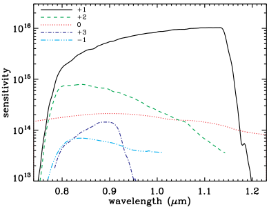
The detector pixels will have a unique sensitivity as a function of wavelength, which in standard direct imaging is calibrated by flat-field images. However for grism observations, the problem is significantly more complex as the wavelength of incident light depends on the position of the source on the detector. Moreover the blending of light from distinct regions leads to a convolution over wavelength, and so the flat-field correction must be taken to be position and wavelength dependent. Additionally, the average pixel response is given by a transmission curve, that transforms the calibrated counts to physical units (in the case of HST data from e^- s^-1 to erg s^-1 cm^-2 Å^-1). We denote this average response as $S(\lambda)$ and show five detectable orders for the G102 grism on WFC3/IR in Figure 1. The pixel-to-pixel deviations from this average response are included in the form of a flat-field “cube”, which is typically given as a polynomial over wavelength whose coefficients encapsulate the spatial variations:

$${\cal F}(x,y;\lambda)=\sum_{i=0}^{n}{\cal F}_{i}(x,y)\left(\frac{\lambda-\lambda_{0}}{\lambda_{1}-\lambda_{0}}\right)^{i},$$ (13)

where $n$ is the order of the flat-field cube, and $(\lambda_{0},\lambda_{1})$ are defined in the calibration process, but are roughly the wavelength coverage of the grism element. The coefficients $\{{\cal F}_{i}(x,y)\}$ are images determined by comparing monochromatic flat-field observations (Kuntschner et al., 2008). We implement three options for the flat-field cube: unity flat (${\cal F}(x,y;\lambda)\!=\!1$), standard cube described by equation (13), and a single direct-image flat-field (e.g. Brammer et al., 2012). These specifications for ${\cal F}_{i}(x,y)$ are suitable for the reconstruction of WFC3/IR grism data, but LINEAR  can handle essentially arbitrary forms for the wavelength-dependent flat field, without significant impacts on the processing.

There are geometric distortions in the detector due to choices in the optical design and imperfections in the manufacture, which causes the effective area of the pixels to vary across the detector. Indeed, for WFC3 much of the geometric distortion is by design, as a result of the desire to minimize the number of reflections while correcting the spherical aberration and maintaining a flat focal plane. The pixel-area maps ${\cal P}(x,y)$ give the area relative to a nominal pixel. For WFC3/IR, the pixel areas change by $\sim\!8\%$ across the detector (e.g. Kalirai et al., 2010).

3 Algorithm

3.1 LINEAR

Inherent to our working paradigm is that there exists direct imaging that satisfies a few requirements:

1. covers $\sim\!2\times$ the area of the instrument to account for sources that disperse onto the detector (see Section 4 of Pirzkal, Ryan, & Brammer, 2016),

2. considerably deeper than any individual grism exposure to minimize double-counting photometric noise and ensure all sources are accounted for, and

3. is at roughly the same wavelength as sampled by the dispersed data to minimize the effect of any wavelength-dependent morphological effects and changes in the point-spread function (PSF).

We implement two options to define the extraction apertures for each source, which we define as the collection of pixels that have a common spectral shape. The first method is to use a classic segmentation map (e.g. Bertin & Arnouts, 1996) with the same world-coordinate system (WCS) as the aforementioned direct imaging. This approach is easy to implement and familiar to many users, but leads to the discrete assignment of each pixel to a source (or the sky). Therefore, our second method allows for the layering of flux densities, associated with multiple sources that potentially overlap in the direct image. This is facilitated by supplying two multi-extension FITS files (MEF); the first expresses the source brightness and second defines the extraction pixels (as a binary image). Each extension of these files must contain an accurate WCS and represents the information for each source, therefore the two images have the same number of extensions. This layered approach additionally facilitates reconstructing spectra for overlapping regions (such as supernova/host galaxy, bulge/disk separation, or overlapping galaxies). Using the MEF data, we also permit the reconstruction parameters (such as spectral sampling) to be different for each source. Both implementations can handle disconnected or island regions and provide the direct image pixel-by-pixel brightness, which is used in the reconstruction process.

Algorithm 1 Computing $W$-matrix Element

1:input: list of dispersed images, direct image, segmentation map, and wavelength resolution

2:for each: dispersed image in image list do

3:     for each: object in segmentation image do

4:         for each: pixel in the object do

5:              transform the pixel corners to dispersed image using WCSs (including distortion)

6:              for each: wavelength associated with the object do

7:                  invert dispersion (equation (4)) to determine path length for given wavelength

8:                  invert path length (equation (5)) to compute $\tilde{x}$-coordinate

9:                  compute $\tilde{y}(\tilde{x})$ from spectral trace (equation (1))

10:                  convert trace to dispersed-image coordinates (equation (2))

11:                  compute overlapping area ($a(\lambda)$) with dispersed image pixel grid

12:                  compute weight (equation (18))

13:              end for

14:         end for

15:         sum weights over unique combinations of $(x,y,\lambda)$

16:         record the object-dispersion table (ODT) of $(x,y,\lambda,W)$

17:     end for

18:end for

19:load the ODTs and sum $w$ in wavelength bins — the bin widths and locations can vary between objects

20:divide weights by image uncertainty for least-squares minimization (see equation (20))

21:sum over unique combinations of $(x,y,\lambda)$ — now have multiple objects to sum

22:output: sparse matrix stored in COO-notation ($\vartheta,\varphi,W_{\vartheta,\varphi}$)

The brightness detected in a dispersed-image pixel is the sum over all sources and wavelengths:

$${\cal G}_{x,y,i}=\sum_{\lambda}\sum_{j}^{N_{\rm obj}}W_{x,y,i,\lambda,j}\,f_{\lambda,j},$$ (14)

where ${\cal G}_{x,y,i}$ is the measured brightness in the $i^{\mathrm{th}}$-grism image at pixel $(x,y)$, $f_{\lambda,j}$ is spectrum for the $j^{\mathrm{th}}$-object, and $W$ is a collection of transformation factors describing the dispersed image signal for a unit spectrum. The value of $W$ includes the flux distribution of the source, and is explicitly summed over all direct-image pixels in the source. For typical sparse fields, many of the $W$-elements will be zero by construction, since only a few sources can contribute flux to a given pixel at a given wavelength. By grouping the measurement (“the knowns”) and spectral (“the unknowns”) indices respectively:

$$(x,y,i) \rightarrow \vartheta$$ (15)

$$(\lambda,j) \rightarrow \varphi,$$ (16)

equation (14) becomes a simple matrix product:

$${\cal G}_{\vartheta}=\sum_{\varphi}W_{\vartheta,\varphi}\,f_{\varphi}.$$ (17)

LINEAR populates the elements of the $W$-matrix by iterating through the canon of dispersed images and objects in the extraction apertures. Since the direct image and segmentation map may have an arbitrary pixelation, it often necessary to subsample the wavelength to ensure that each dispersed image locations represents, with sufficient fidelity, the spectral energy distribution (SED) of each source. We implement the subsampling as an integer number of steps smaller than the native spectral resolution: $\delta\lambda\!\approx\!N^{-1}\,\mathrm{d}\lambda/\mathrm{d}s$, where $\mathrm{d}\lambda/\mathrm{d}s$ is the field-averaged dispersion for the detector (for WFC3/G102 it is $\mathrm{d}\lambda/\mathrm{d}s\!\approx\!25$ Å pix^-1) and $N$ is the subsampling factor. We explored various choices for the subsampling factor, but found that $N\!=\!5$ is a good compromise between computational constraints and spectral fidelity for a direct image with pixels $\sim\!16\times$ smaller than the native detector (for WFC3/IR the native pixel scale is $\sim\!0\farcs 12$). However we caution that the best value of $N$ likely varies on the properties of the direct imaging in question.

In this formalism, $W$ is a linear operator that transforms the spectra $f_{\varphi}$ into the observed pixel brightnesses ${\cal G}_{\vartheta}$. The bulk of the processing for LINEAR is computing the $W$-matrix elements; we summarize these calculations in Algorithm (1). The matrix elements (weights in the linear equations) are given as a product of the instrumental effects described above:

$$W=a(\lambda)\,{\cal I}(x_{0},y_{0})\,{\cal F}(x,y;\lambda)\,{\cal P}(x,y)\,S(\lambda)\,\delta\lambda$$ (18)

where $a(\lambda)$ is the relative pixel area from the reprojection at some wavelength, ${\cal I}(x_{0},y_{0})$ is the normalized image brightness from the direct image, ${\cal F}(x,y;\lambda)$ is the flat field, ${\cal P}(x,y)$ is the correction from the pixel-area map, $S(\lambda)$ is the average sensitivity curve, and $\delta\lambda$ is the subsampled bandwidth.

The optimal set of object spectra will minimize the goodness-of-fit metric derived from maximizing a Gaussian likelihood:

$$\chi^{2}=\sum_{\vartheta}\left(\frac{\sum_{\varphi}W_{\vartheta,\varphi}f_{\varphi}-{\cal G}_{\vartheta}}{{\cal U}_{\vartheta}}\right)^{2}$$ (19)

where ${\cal U}_{\vartheta}$ is the estimated uncertainty for datum $\vartheta$. These uncertainties can be factored into the $W$-matrix and the pixel-by-pixel flux measurements (${\cal G}_{\vartheta}$) as:

$$W_{\vartheta,\varphi} \rightarrow W_{\vartheta,\varphi}/{\cal U}_{\vartheta}$$ (20)

$${\cal G}_{\vartheta} \rightarrow {\cal G}_{\vartheta}/{\cal U}_{\vartheta}.$$ (21)

Equation (19) can be extended to a damped-least squares in a simplified-matrix notation of:

$$\hat{f}=\underset{f}{\operatorname{arg\,min}}\left(||W\,f-{\cal G}||^{2}+\ell\,||W||_{F}^{2}\,||f||^{2}\right),$$ (22)

where $\hat{f}$ is the optimized solution, $||W||_{F}$ is the Frobenius norm of $W$, and $\ell$ is a damping parameter that imposes smoothness in the final solution. We defer discussion of the damping parameter and its effects to Section 4.2 and Section 5. Unlike most presentations, we include the Frobenius norm in the second term so that the damping parameter is dimensionless.

The size of the $W$-matrix will be the number of knowns by the number of unknowns. The number of knowns is the total number of pixels analyzed, which includes all the pixels that contain source flux (that may be as large as the number of images times the number of pixels per image, but is generally less). The number of unknowns is roughly the number of objects times the number of flux elements per object (to be clear, LINEAR allows the number of flux elements to be different for each object). For a deep dataset with WFC3/IR (e.g. Pirzkal et al., 2017), there may be $\sim\!100$ images with $\sim\!10^{6}$ pixels each (but only $\sim\!10\%$ of these pixels may have source flux) to extract $\sim\!1000$ objects for $\sim\!100$ spectral elements. Therefore the $W$-matrix will have dimensionality of $10^{7}\times 10^{5}$, however the vast majority ($\gtrsim\!99.9$%) of these elements are exactly zero, since any one source will affect only a small fraction of pixels on any one dispersed image at any wavelength. Therefore we employ several sparse-matrix techniques, specifically storing the $W$-matrix in the coordinate-list (COO) format and use the LSQR algorithm (Paige & Saunders, 1982).

The LSQR algorithm estimates the uncertainty on the parameters (i.e. the reconstructed spectra in this case), however these values will be underestimated for $\ell\!\neq\!0$. Paradoxically, a very large damping parameter implies vanishingly small uncertainty, as the optimization depends only on the variance of the reconstructed spectra; so that equation (22) becomes:

$$\hat{f}=\underset{f}{\operatorname{arg\,min}}\left(||f||^{2}\right)$$ (23)

when $\ell\!\rightarrow\!\infty$. Therefore, the optimal solution will be when all elements of $f$ are exactly zero. To account for this, we implement a Markov Chain Monte Carlo (MCMC) simulation to sample from the likelihood, which is given by $\ln(L)\!=\!-\chi^{2}/2$ (see equation (19) for the definition of $\chi^{2}$). In many cases, this will be of exceedingly high dimensionality, therefore we compute the uncertainties for each source sequentially by holding the spectra of the remaining sources fixed to the values found by solving equation (22) with LSQR. Our sequential uncertainty analysis is formally correct for the limiting case of no overlapping dispersions, but does not include any correlations induced by overlapping spectra. We have verified the uncertainty estimates coming from the MCMC sampler are consistent with the uncertainties reported by other means (e.g. Pirzkal et al., 2017). We further discuss additional details of the damping parameter in Section 4.2.

The majority of the code is written in IDL with the exception of two key steps: (1) the area computations are performed via the Sutherland-Hodgman algorithm with C code provided by J. D. Smith (as developed for CUBISM: Smith et al., 2007), and (2) we translated the scipy implementation of the LSQR algorithm into C. However, both components can default to IDL-only implementations if the C code is not successfully compiled. We have integrated the multithreading package OpenMP into the components that are written in C, but provide non-threaded versions for simplicity.

3.2 Bad Pixels and Additional Spectral Orders

It is important to note that we remove all pixels from $\{{\cal G}\}$ that are flagged in the bad-pixel masks (BPXs) or having flux coming from additional spectral orders. To identify pixels from additional orders, we follow a very similar procedure to that described in Algorithm 1, however to expedite the calculations we do not consider each pixel belonging to an object, but rather group the pixels into a convex hull. This would amount to a considerable loss in spectral fidelity if this prescription were used for building the $W$-matrix.

3.3 Additional Capabilities

The vast majority of the processing efforts for LINEAR deal with populating the $W$-matrix elements. However once $W$ is fully formed, there are many useful calculations that can be readily performed:

• predicting contamination estimates — valuable for planning observations of a select number of high-value science targets;

• providing average wavelength for sources; and

• excising two-dimensional grism images for sources.

As these are not the primary goal of this work, we defer detailed discussion of their usability to the LINEAR  reference manual provided with the codebase (Ryan, Casertano, & Pirzkal, 2016).

3.4 Preprocessing

LINEAR  simply represents a new paradigm for reconstructing one-dimensional spectra from a canon of dispersed images, and several pre-processing steps must be performed.

3.4.1 Background Subtraction

The sky background in a grism image is far more complex than standard direct imaging, and is typically estimated by fitting a master sky image to the sky pixels in an image (as discussed in Pirzkal et al., 2004). This inherently assumes the sky flux is dominated by a single spectral component, whereas Brammer et al. (2014) demonstrate that for WFC3/IR there are at least two distinct spectra contributing to the sky background (e.g. zodical light and He I emission). Therefore the fitting process becomes quite a bit more complex (see the § 6. Appendix: Iterative Inversion of Brammer, Ryan, & Pirzkal, 2015). This becomes even more problematic should one of the spectral components vary with time, and the standard ramp-fitting in infrared detectors must be incorporated in sky background modeling (e.g. Pirzkal & Ryan, 2017b). Since it is impossible to predict which algorithm (single master sky, multiple sky components, time-variable components) a dataset might require, we instead assume the images have been background subtracted by some means. In Section 4.1.2, we show how residual levels of flux will adversely affect the quality of the extracted spectra.

3.4.2 Astrometric Registration

As described in Section 2, HST grism observations typically include obtaining a shallow pre-image to accompany each dispersed image (or set of dispersed images with known dithers) to refine the astrometry of the dispersed data. There are numerous tools available for such processing (such as Gonzaga et al., 2012; Avila et al., 2015), and so we do not attempt any astrometric corrections. The possible impact of registration errors is discussed in Section 4.1.1.

If the direct and dispersed images are not taken at the same time (as may be the case for the WFIRST High-Latitude Survey: HLS; Spergel et al., 2015), then appropriate preprocessing must be carried out to ensure that the direct and dispersed images are correctly aligned. Some concepts and methods to this end have been discussed or developed by Dixon (2016) and Bohlin, Deustua, & Pirzkal (2015).

4 Tests of LINEAR

For the following tests of LINEAR, we consider observations from the Hubble Space Telescope using the Wide-Field Camera 3 with the G102 grism element with pre-imaging through the F105W filter. For all of the tests described below, we use LINEAR to generate simulated grism images through the G102/F105W combination, which includes the best available estimates of the spectral trace, dispersion, field edges, average sensitivity, wavelength-dependent flat field, and the pixel-area map. By accounting for filter-wedge offsets (Sabbi, 2012), it is possible to consider other grism/filter combinations (Pirzkal, Ryan, & Brammer, 2016). In Figure 1, we show the field-averaged sensitivity of the G102 element to set the stage.

Figure 1: The sensitivity curves for HST WFC3/G102 in units of e^- s^-1 per erg s^-1 cm^-2 Å^-1. Each line represents a different spectral order, as described in the upper left: $+1^{\mathrm{st}}$ (solid black), $+2^{\mathrm{nd}}$ (dashed green), $0^{\mathrm{th}}$ (dotted red), $+3^{\mathrm{rd}}$ (dot-dashed purple), and $-1^{\mathrm{st}}$ (dot-dot-dot-dashed cyan).

4.1 Uncertainties and Error Propagation

Below we describe a series of Monte Carlo simulations designed to assess the impact of the uncertainties in the calibrations on the final spectroscopy. In each simulation, we consider a single Gaussian point source with a flat spectrum in $f_{\lambda}$.

4.1.1 Astrometric Registration

Since we are extracting the spectra on a native pixel scale, the precise registration of the dispersed image to the existing images is crucial. We simulate a Gaussian object for four distinct orients $\{0^{\circ},90^{\circ},180^{\circ},270^{\circ}\}$ with no photometric noise (as the goal here is to isolate the effects of astrometry, and photometric noise will be considered below). We add a Gaussian random offset to the CRVAL keywords to simulate an error in the astrometric registration, and reconstruct the one-dimensional spectrum with the LINEAR algorithm. We repeat this procedure many times and show the average (red dashed) and standard deviation (gray region) as a function of wavelength in Figure 2. The input spectrum is shown in black and the standard deviation of the Gaussian offset in native pixels is given in the lower left corner of each panel.

Figure 2: The relation between astrometric registration and spectrophotometric uncertainty. In the upper left corner of each panel, we give the uncertainty in the CRVAL keywords in units of native pixel scale ($\sim\!0\farcs 12$). For this Monte Carlo simulation (described in Section 4.1.1), we consider a single Gaussian point source with a flat spectrum in $f_{\lambda}$ (black line) observed at four orients. By simulating this configuration many times with Gaussian noise added to the astrometry, we synthesize the average spectrum (red dashed line) and standard deviation (gray region) as a function of wavelength. For typical HST/WFC3 observations, the astrometry is easily refined to $\sim\!0.1$ pix and therefore LINEAR  is not expected to introduce any significant ($\lesssim\!0.1\%$) additional spectrophotometric noise.

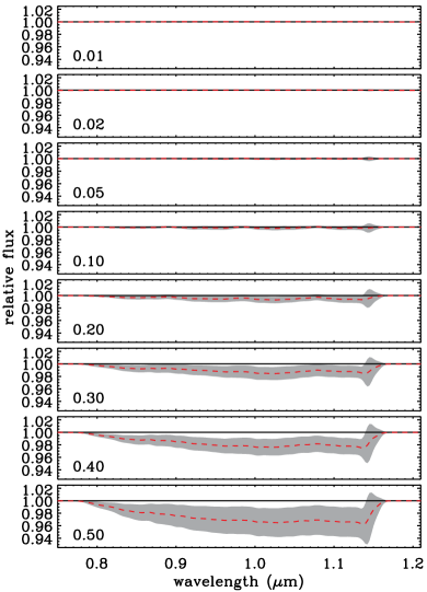
For most realistic situations, it is fairly straight-forward to astrometrically align images to the $\sim\!0.1$ pix in the case of WFC3/IR. Based on our Monte Carlo simulation, we estimate this astrometric uncertainty introduces an error of $\lesssim\!1$%. We also find that for the wavelengths with high sensitivity ($0.8\!\lesssim\!\lambda\!\lesssim\!1.1~{}\mu$m), the typical photometric uncertainty scales like $\sigma_{f}\!\approx\!0.03\,\sigma_{r}$, where $\sigma_{r}$ is the offset in the astrometry in native pixels (i.e.  the values listed in the lower-left corner of each panel in Figure 2) and $\sigma_{f}$ is uncertainty on the spectrum for a source brightness of $Y\!=\!18$ mag.

4.1.2 Background Subtraction

Figure 3: The effect of residual background level on spectral uncertainty. In the upper left corner of each panel, we give the uncertainty for the background level in $e^{-}$ s^-1. We describe this simulation in Section 4.1.2. Here the colors, plot symbols, and axes are the same as in Figure 2. Based on a collection of WFC3/IR data, Pirzkal & Ryan (2017b) estimate a typical residual level of $\sim\!0.01$ $e^{-}$ s^-1, therefore the typical induced spectral uncertainty is $\sim\!0.1\%$.

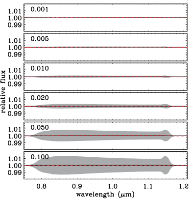
We now consider the Gaussian source through the same four orients, but impose a Gaussian random pedestal sky brightness. For each sky background uncertainty, we generate 100 realizations of the four orients. In Figure 3, we show the averaged extracted spectrum, and the colors and plot symbols have the same meaning as in Figure 2. In a recent Instrument-Science Report (ISR), Pirzkal & Ryan (2017b) demonstrate that one can remove the sky background levels to $\sim\!0.01$ e^- s^-1 using a constant zodical background and time-varying helium emission model (Brammer et al., 2014). Following that prescription, we estimate the inaccuracies introduced from improper background subtraction to be $\sim\!0.1\%$. We find that the photometric uncertainty scales roughly as the background subtraction uncertainty: $\sigma_{f}\!\approx\!0.13\,\sigma_{B}$.

It may be possible to further reduce the background subtraction accuracy to $\sim\!0.001$ e^- s^-1 with a smoothed, column-averaged correction and/or global mean (e.g. Pirzkal et al., 2017). Since the typical background accuracy is already a sub-dominant term in the uncertainty budget, we do not carry out further corrections. In Section 6, we discuss possible modifications to our algorithm that may provide such refinements in the background.

4.1.3 Photometry and Signal-to-Noise

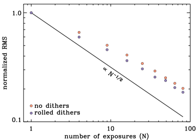
To assess the relationship between total exposure time (or number of images) and inferred signal-to-noise, we consider the same source with flat spectrum in $f_{\lambda}$ as described above. However here we explicitly include Gaussian random noise consistent with a $1200$ s exposure with G102 on WFC3/IR. We create $N$ images of this scenario and extract the spectrum, then repeat for 100 realizations of these images to estimate the variance for a fixed number of input images. We consider two cases for the orientation of the $N$ images: (1) perfectly coaligned, with no rotation; and (2) rotated by $N$ different angles, uniformly distributed in the range $[0,2\pi]$. We repeat this procedure for different values of the number of images $N$, ranging from 1 to 100. Figure 4 shows the resulting spectrophotometric uncertainty, expressed as the root-mean square (RMS), averaged in bins of wavelength, as a function of $N$, scaled to the single-image value. We find that the RMS error scales approximately as $N^{-0.4}$ for both the case with no rotation (red points) and with uniformly distributed rotations (blue points).

Figure 4: Spectrophotometric uncertainty. As described in Section 4.1.3, we consider a series of $N$ independent exposures, each with noise consistent with a $1200$ s image in WFC3/G102. We then extract the source in various combinations of these images to show the decrease in spectrophotometric uncertainty with exposure time. The red and blue points show the uncertainty for undithered and roll-dithered images, respectively. The solid black line represents the standard scaling of $\propto\!N^{-1/2}$, and each set of points are normalized to unity at $N\!=\!1$. The simulated data scale more shallowly ($\propto\!N^{-0.4}$).

4.2 The Effect of Damping

The damping coefficient $\ell$ in equation (22) applies a penalty to solutions of $\{f\}$ that have high variance, which has the effect of damping high-frequency oscillations. In the case of equation (22), the oscillations are damped with respect to $f\!=\!0$ (for all elements of $f$), but this can be extended to an arbitrary damping target ($f_{0}$) as

$$\hat{f}^{\prime}=\underset{f^{\prime}}{\operatorname{arg\,min}}\left(||W\,f^{\prime}-{\cal G^{\prime}}||^{2}+\ell\,||W||_{F}^{2}\,||f^{\prime}||^{2}\right),$$ (24)

where $f^{\prime}\!=\!f-f_{0}$, ${\cal G^{\prime}}\!=\!{\cal G}+W\,f_{0}$, and $\hat{f}\!=\!\hat{f}^{\prime}+f_{0}$. To visualize the effect of damping, we consider four SEDs that serve to highlight the range of effects typical in many grism surveys: a constant in $f_{\lambda}$, an L5V brown dwarf, a step function with break at $\lambda_{\rm obs}\!=\!1~{}\mu$m, and an emission line source with line at $\lambda_{\rm obs}\!=\!1~{}\mu$m (the line has a Gaussian profile and an observer-frame equivalent width of $W_{\rm obs}\!\approx\!-50$ Å). In all cases, we implement a Gaussian source profile normalized to $Y\!=\!18$ mag that is observed in 100 dithered images, each having realistic noise. We extract the spectrum for each SED with various damping parameters $\ell\!\in\!\{0,0.01,0.05,0.1,0.2,0.5,1,2,5,10,20,100\}$, damped to a constant $f_{\lambda}$ of $Y\!=\!18$ mag ($f_{\lambda}\!\approx\!6.1\times 10^{-17}$ erg s^-1 cm^-2 Å^-1), and iterate this procedure 100 times to estimate the variance around the mean. In Figure 5, we show the extracted spectra, averaged over the 100 iterations, with each value of $\ell$ indicated by a different color; the black line represents the input spectrum. The red lines show the spectrum extracted with $\ell\!=\!0.01$, which clearly reproduce the input (black line) spectra the best. However, they also show the largest variance around the mean, and so we consider these the hot extractions. On the other hand, the blue lines ($\ell\!=\!100$) are highly smoothed versions of the input (i.e.  the damping target $f_{0}$). In fact, these cold extractions are so damped, they are often flat spectra close to the average brightness.

Figure 5: Effect of the damping parameter on the extracted spectrum of a Gaussian source. The four panels are split into a top and bottom sub-panel that show the average and RMS spectrum, respectively, for different input spectra, represented by a black line (top left: step function, top right: constant with emission line, and bottom right: L5V brown dwarf). These sources were extracted with a range of damping parameters ($\ell$, see equation (22)), as indicated with the color bar.

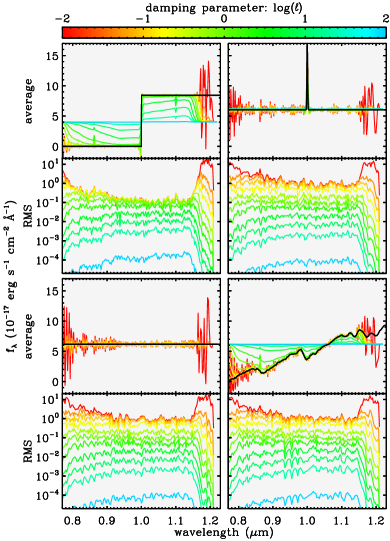
This simulation raises a challenging question: How to select the ideal value for $\ell$? After all, spectra reconstructed with little damping (small $\ell$) are close to the input spectrum (i.e. the damping target) at the cost of increased noise from the inversion process. Moreover, LSQR may bias the extracted toward the damping target for $\ell\!\gg\!0$; see the blue spectra plotted in Figure 5, particularly the top left panel. This effect arises when the damping target is a poor match to the underlying spectrum, which is generally unknown in the reconstruction phase.

Hansen (1992) reviews analysis of the L-curve, a plot of $\log||Wf-{\cal G}||^{2}$ and $\log||f||^{2}$ that is parameterized by $\ell$, that offers a compromise between fitting the observations and damping fluctuations. The point where the local curvature is maximum is considered the optimal damping parameter in reconstructing the incident spectra. Cultrera & Callegaro (2016) present an iterative algorithm for locating this critical point based on the golden-section search method. At this time, we do not implement this approach; instead we sweep through a range of the damping parameter to locate the critical point, as discussed in Section 5.

Following the preceding discussion in Section 3.1, the LSQR algorithm formally provides a mechanism for computing the variance of the solution. Now for a non-zero damping target $f_{0}\!\neq\!0$, the optimal solution is no longer identically zero, but rather approaches $f_{0}$. The concern that LSQR significantly underestimates the true uncertainty is still present, and so the uncertainty derived from the MCMC sampling is preferred.

4.3 Multiple Sources and Overlapping Traces

Figure 6: Illustrative example of spectral confusion for two sources. Here we consider two Gaussian sources (shown in the insets as red and blue) whose relative position in the sky is fixed, but we view them under two different position angles (top and bottom figures). The $1^{\mathrm{st}}$ order traces of each source is shown in its corresponding color (the colors here are chosen to highlight the overlap and do not refer to the spectral shape of either source). In the bottom panel, the $1^{\mathrm{st}}$ order dispersions from the two sources considerably overlap, leading to a region of spectral confusion (as indicated with the green rectangle). However when these objects are observed at a different position angle, then their dispersions do not overlap, yielding two unconfused $1^{\mathrm{st}}$ order traces. This example provides the main motivation behind the development of this algorithm.

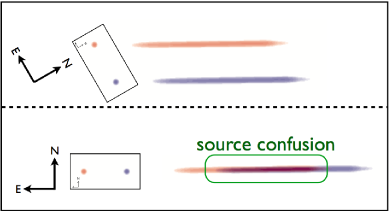
One of the key goals of LINEAR is to better address the issue of contamination when the trace of multiple sources overlap on the detector. To detail the success of LINEAR  in this regime, we consider a Monte Carlo simulation similar to those described in previous sections. Here we simulate two sources with $Y\!=\!18$ mag that are separated $1\farcs 5$ and have a step-like and L5V spectra as described above. In Figure 6, we show an illustrative example of the two sources observed in two position angles (for simplicity we plot the sources here with constant SEDs: $f_{\lambda}\!=\!f_{0}$). Based on this intrinsic scene, we create five observational scenarios, each of which consists of four distinct grism images. We dither these four images according to the WFC3-IR-DITHER-BOX-MIN pattern (Table C.3 of Dressel, 2017). Each scenario has a different distribution of position angles (PAs; see Table 1) designed to bracket the primary possibilities:

fully degenerate

the sources overlap in all spectroscopic images; such as the case in single orient, but possibly dithered, data (e.g. Atek et al., 2010; Brammer et al., 2012). It is worth noting that, this situation may also arise in the case of data taken in two orients that are offset by $180^{\circ}$;

partially degenerate

the sources overlap in some images, but are uncontaminated in others; such as the case with data taken at multiple orients, but possibly with dithers at a given orient (e.g. Pirzkal et al., 2004, 2017); and

non-degenerate

sources overlap in no spectroscopic images; such as the case of distinct sources, to be considered as a null hypothesis.

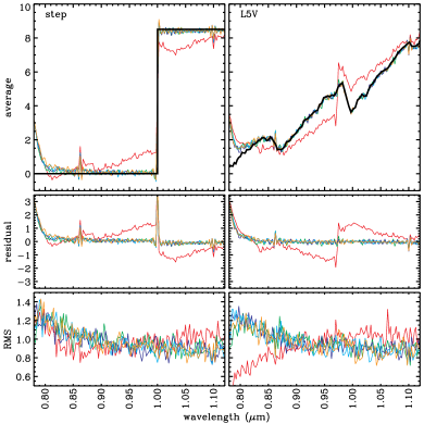
For each simulated grism image, we include background noise consistent with a $1200$ s exposure with G102 on WFC3/IR, complete with the effects described in Section 4. We simultaneously reconstruct the two spectra from all four images (within a given observational scenario), and iterate this process 100 times. In Figure 7, we show the extracted spectra for the five scenarios, each of which is averaged over the 100 iterations. The colors of the lines are described in Table 1.

LINEAR is quite adept at reconstructing the overlapping dispersions, provided at least some of orients are uncontaminated. In fact, the difference between the partially-degenerate scenarios (#3, 4, 5) and non-degenerate scenario (#2) are relatively minor. Furthermore, LINEAR  cannot reconstruct the spectra of the sources in the fully-degenerate scenario (#1), which is to be expected. In the fully-degenerate scenario, LINEAR  tends to produce very similar spectra for the two sources, which have features that are indicative of both objects. For example, the step-like and strong molecular absorption of the intrinsic spectra are evident in the fully-degenerate case. This highlights the importance of having multiple orients, however more work is needed to estimate the appropriate number or distribution of orients for an arbitrary (or specified) scene.

Table 1: Position Angles

scenario	PAs	color
	(deg)
1	0,0,0,0	red
2	0,30,60,90	green
3	0,0,90,90	blue
4	0,0,0,90	cyan
5	0,45,45,90	orange

Figure 7: Spectral reconstruction of two overlapping dispersions. As described in Section 4.3, we consider five scenarios that vary the degree of degeneracy between the two sources, as modulated by the distribution of position angles (see Table 1). In the top, middle, and bottom panels we show the average, residual, and RMS (respectively), which are computed from the 100 iterations (see Section 4.3). In the top panels, we indicate the input spectra used for computing the residuals, otherwise the line colors are given in Table 1. For the maximally-degenerate scenario (#1), LINEAR is clearly incapable of reconstructing the spectra for the sources with any confidence. In contrast, the partially-degenerate scenarios (#3, 4, 5) do not perform demonstrably worse than the fully-non-degenerate scenario (#2), which we consider to be the null hypothesis.

5 A Case Study: The Hubble Ultra-Deep Field

To demonstrate the power of LINEAR, we present the WFC3/IR grism spectroscopy of the Hubble Ultra-Deep Field (HUDF; Beckwith et al., 2006). There are two programs that observed the HUDF in the G141 grism; we briefly summarize the key properties of these data in Table 2. We process these data using standard algorithms implemented by CALWF3, but apply additional time-variable background sky subtraction as described by Pirzkal et al. (2017). However, the G141 data can have an additional time-variable spectral component coming from earth-glow (e.g. Brammer et al., 2014, but also discussed above in Section 3.4.1). We use the contemporaneously obtained pre-imaging in the F140W band to refine the astrometry of the grism images, and provide the direct image for the pixel weights (${\cal I}(x_{0},y_{0})$ in equation (18)). However, one of the visits for program 12177 required higher than normal background corrections, therefore, to avoid contaminating this case study, we exclude these four exposures ($\sim\!5320$ s) from our analysis. This results in 36 individual images, obtained over three orients, for a total integration time of $\sim\!43.31$ ks. However with the relative positions and field rotations, not every source has this total exposure time. In principle, this results in $\sim\!4\times 10^{7}$ independent measurements, since the WFC3/IR detector is $1014\times 1014$ pix². However the number in practice is $\sim\!1.92\times 10^{6}$, since only a fraction of the useable pixels contain source flux.

Table 2: HUDF Grism Observations

PropID	ORIENTAT	Exp. Time
	(deg)	(ks)
12099	$-178$	$15.04$
12177	$+176$	$18.85$
	$+127$	$9.42$

We extract one-dimensional spectra for sources with F140W$\!\leq\!26$ mag (as defined by an isophotal magnitude described in Pirzkal et al., 2017), which resulted in $1,112$ individual sources. For each source, we extract between $1.0\!\leq\!\lambda\!\leq\!1.7~{}\mu$m with a sampling of $50$ Å  ($120$ elements per source), which results in $\sim\!1.1\times 10^{5}$ unique spectral elements to be determined by LINEAR. The $W$-matrix has $\sim\!3.82\times 10^{8}$ non-zero elements for a sparsity of $\sim\!0.017$% and a Frobenius norm of $||W||_{F}\!=\!8.2\times 10^{4}$ e^- s^-1 per $10^{-17}$ erg s^-1 cm^-2 Å^-1. For comparison, we also extract the sources through the same apertures using standard techniques (e.g. Pirzkal et al., 2017), and then average combine with inverse-variance weights the three orients for each source.

Figure 8: The L-curve for the G141 spectroscopy from the HUDF as described by Hansen (1992). This analysis provides a mechanism for selecting the optimal damping parameter as a compromise between modeling the data and fluctuations in the resulting spectra, as indicated by the abscissa and the ordinate, respectively. The color of the line indicates the parametric value of the damping, as indicated by the color bar in the upper right corner. In the inset to the lower left, we show the curvature as a function of the damping that is used to select the optimal damping parameter ($\ell_{\rm opt}$), which we indicate with the bullseye.

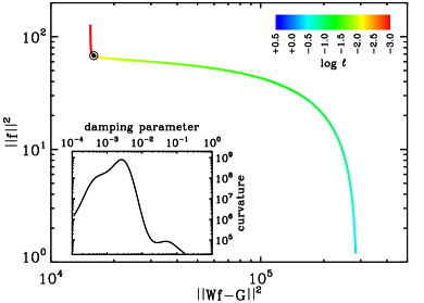
We show the L-curve (as Section 4.2) for these G141 data in Figure 8, and the color of the line indicates the value of the damping parameter, as shown in the color bar. Although there are algorithms for efficiently locating the point of maximum curvature (e.g. Cultrera & Callegaro, 2016), we simply sweep through a range of damping parameters to compute the point of maximum curvature, as shown in the inset to Figure 8. From this we find an optimized damping parameter of $\ell_{\rm opt}\!=\!2.57\times 10^{-3}$, which is the value we adopt for all subsequent analyses. In Figure 9, we show several sources with strong emission lines, whose colors are described in the caption.

Figure 9: Illustrative examples of LINEAR  from the G141 spectroscopy from the HUDF arranged by spectroscopic redshift. The blue and red lines represent the standard, orient-averaged and LINEAR spectra, respectively. Along the right column, we show the F140W image used to establish the pixel weights. We show the redshifted wavelengths of common optical emission lines as colored vertical dashed lines, but the most common species are [O II] (black), H$\beta$ (green), [O III] (blue), He I (red), H$\alpha$ (cyan), and [S II] (orange). In Figure 10, we show zoomed versions of panels (b) and (d) for clearer illustrations.

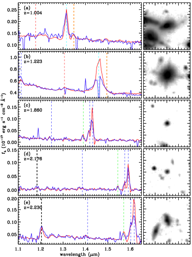
Based on these data in the HUDF, we identify multiple ways in which LINEAR improves upon the orient-averaged extractions. First, the spectral resolution for the LINEAR spectra is $\sim\!20-30\%$ higher than the averaged spectra. This improvement is most pronounced in panels (c), (d), and (e) of Figure 9, where the [O III] and H$\beta$ complex is very clearly resolved (see right panel of Figure 10 for a better representation). This effect arises for two reasons. First, the achievable spectral resolution is limited by the spatial profile projected along the dispersion axis. But since there are several orients, which generally have different projected spatial extents, the individually extracted spectra will have different effective resolutions. Therefore the weighted averaging increases the overall signal-to-noise at the expense of degrading the high-resolution spectra from the high-resolution orients. Second, LINEAR projects and deforms pixels from the direct image to the set of grism images as a function of wavelength to compute the fractional pixel areas. Since each of the grism images have a unique dither position and orientation, they provide a more complete spectral sampling. This is in analogy to drizzling dithered images to improve the spatial resolution (e.g. Fruchter & Hook, 2002; Koekemoer et al., 2003). As a final note, the net improvement in the spectral resolution depends on the geometry of the scene, source(s), and observation(s), therefore we expect these improvements will vary from dataset to dataset.

Figure 10: Zoomed plots of panels (b) and (d) from Figure 9. The colors and symbols have the same meaning as in Figure 9. Here the shape and structure of the He I (left) and the H$\beta$/[O III] complex (right) is seen in better detail, which reinforces the advantages discussed in Section 5.

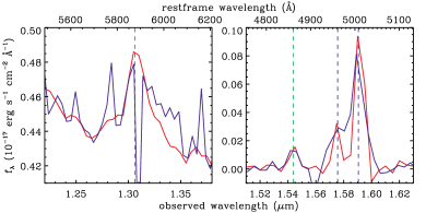
A second advantage of LINEAR  concerns the signal-to-noise, which improves by $\sim\!20-30\%$. For example, the object shown in Figure 9(b) or left panel of Figure 10 is a known quasar based on the X-ray flux and spectroscopic redshift (of $z\!=\!1.22$; Xu et al., 2007; Xue et al., 2011). So here the improvement to the spectral resolution is less profound, however the increased signal-to-noise makes the He I emission at $\lambda_{\rm obs}\!=\!1.304~{}\mu$m easily detectable. LINEAR provides these gains since we model each grism image simultaneously, as opposed to stacking grism images of the same orient (but dithered). This improves the statistics by providing more independent measurements of the underlying signal.

Finally, the first source in Figure 9(a) shows both improvements in signal-to-noise and spectral resolution, but importantly this source is member of a very complex grouping of interacting galaxies. Consequently, it has significant contamination from the neighbors, however LINEAR  is able to faithfully remove these extraneous signals.

6 Subjects for Future Study

As demonstrated, LINEAR  is already quite powerful, however we foresee several modifications in the near future.

1. The current implementation of LINEAR is highly geared toward WFC3/IR, however it would be straight-forward to include the other instruments on HST and the planned missions of JWST and WFIRST. At present, LINEAR  is only capable of working with grism configurations in the aXe-based format. As described in Section 2, modifications may be implemented to work with the generalized transformations (see equation (10)) for instruments with row/column dispensers (as with the instruments with The James Webb Space Telescope, see Pirzkal & Ryan, 2017a) or with multiple detectors, particularly if the trace from a single order extends on multiple detectors (such as with WFIRST).

2. It is important to remove the astrophysical background light, and as Brammer, Ryan, & Pirzkal (2015) describe, this can be a non-trivial process. However, the flux coming from the background can be considered as an additional source with a distinct spectrum. Therefore it is formally possible to perform background subtraction within the LINEAR methodology, at the expense of making the $W$-matrix considerably denser in some rows/columns. A first step is to implement a gray background spectrum for each grism exposure, which would add little complexity, but may improve the reconstruction of faint sources that have brightnesses comparable to the background errors.

3. We have framed the problem of reconstructing grism spectroscopy as solving a system of sparse, linear equations, and therefore the optimal set of source spectra can be easily obtained by standard computational techniques. These obvious advantages in solving for the ideal non-parametric spectra are offset by the introduction of a damping parameter. However it may be possible to introduce a limited number of non-linear parameters, which would likely modulate global properties of the reconstruction (such as something that governs the sky background). This additional complexity may require subsuming the LSQR-based minimization in a single step of a non-linear optimizer (such as Levenberg-Marquardt), which solves for these additional parameters.

4. It may be additionally possible to restrict the scope of the LSQR-based matrix solution by only considering sources that overlap in the dispersed images. This would be analogous to solving a friends-of-friends-type problem, where each separate set of friends is solved in parallel. This approach may be implemented by matrix operations on $W$.

5. Because WFC3/IR non-destructively samples the reads, any incident cosmic rays can be flagged by linear regression. The current WFC3/IR calibration software implicitly assumes that there are no time-dependent signals (such as the sky background varying with time), which can easily confound the cosmic ray flagging (e.g. Brammer, Ryan, & Pirzkal, 2015; Brammer, 2016; Pirzkal & Ryan, 2017b). Additionally, optical detectors (such as the Advanced Camera for Surveys) will not have the non-destructive sampling and, therefore may require additional processing steps in the reconstruction to remove the cosmic rays.

7 Discussion

The LINEAR  algorithm leverages all of the spectral information at the reconstruction phase to produce the best one-dimensional spectrum consistent with the data. We foresee several situations where the LINEAR paradigm will be a major improvement over standard algorithms for analyzing slitless spectroscopy.

crowded fields

Standard extraction tools simply flag regions of a two-dimensional dispersed image that have contributions from multiple sources. In a future work, we present a use-case for spectroscopy of high-redshift sources lensed by foreground galaxy clusters (Ryan et al. 2018, in preparation). LINEAR  may be equally adept at spectroscopy in dense stellar fields, however further tests may be necessary to establish the number of orients needed for complete spectroscopic coverage.

spatially resolved spectroscopy

We have framed the notion of a source as a collection of pixels assumed to have a consistent spectral shape. Importantly, these collections may be associated with a single physical object, such as a large, resolved galaxy or nebulosity. Therefore it may be possible to partition a single astrophysical object into many sources, and LINEAR will be capable of extracting individual one-dimensional spectra separately for each partition. In this way, LINEAR may approximate slitless spectroscopy as an integrated-field unit (IFU). However, it will be important to keep certain statistical issues in mind, such as the relative numbers of knowns and unknowns (as discussed in Section 3.1).

strict sampling requirements

It may be that a survey has very strict requirements on any completeness and/or reliability of the extracted spectroscopy or the derived products (such as redshift). For example, the various cosmology experiments with WFIRST place stringent expectations on the spectroscopic redshift accuracy and completeness (or sample size; Spergel et al., 2015). Furthermore strong positional biases in the redshift quality, whether they stem from the quality of existing photometry to make a crude estimate of photometric redshift (e.g. Brammer et al., 2012) or confusion/contamination from crowded regions, is important to characterize and resolve. Therefore an entirely self-contained framework that does not rely on existing photometry like LINEAR will be an important analysis technique.

8 Summary

We have presented a new algorithm for extracting slitless spectroscopy, and demonstrated the success with archival HST WFC3/IR data. This algorithm was devised to explicitly correct for overlapping dispersions and circumvent the need for contamination corrections. In forthcoming works, we will show additional use cases, particularly regarding the mitigation of contaminating sources.

Appendix A Notation Glossary

To avoid any confusion with the above notation, we provide a glossary to define the key variables and their units.

Table 3: Notation Glossary

symbol	units	explanation
${\cal G}_{i}$		the $i^{\mathrm{th}}$ grism image
${\cal G}_{x,y,i}$ or ${\cal G}_{\vartheta}$	e- s-1	the measured brightness at pixel $(x,y)$ in the $i^{\mathrm{th}}$ grism image
${\cal U}_{x,y,i}$ or ${\cal U}_{\vartheta}$	e- s-1	the measured uncertainty at pixel $(x,y)$ in the $i^{\mathrm{th}}$ grism image
$\tilde{y}(\tilde{x})$	pixel	spectral trace in relative coordinates
$S(\lambda)$	e- s-1 per erg s-1 cm-2 Å-1	field-averaged sensitivity as a function of wavelength
${\cal F}(x,y;\lambda)$	dimensionless	flat-field cube
${\cal F}_{j}(x,y)$	dimensionless	the $j^{\mathrm{th}}$ component for the flat-field cube coefficients
${\cal I}_{i}(x,y)$	dimensionless	normalized, direct image of the $i^{\mathrm{th}}$ source
$f_{\lambda,j}$ or $f_{\varphi}$	$10^{-17}$ erg s-1 cm-2 Å-1	calibrated spectrum for the $j^{\mathrm{th}}$ source
$f$	$10^{-17}$ erg s-1 cm-2 Å-1	collection of computed spectra — the same as $f_{\lambda,i}$ but flattened into a single array
$\hat{f}$	$10^{-17}$ erg s-1 cm-2 Å-1	optimized solution for the set of source spectra
$f_{0}$	$10^{-17}$ erg s-1 cm-2 Å-1	collection of damping targets — the same dimensionality as $f$
$s(\tilde{x})$	pixel	path length along the spectral trace
$(x,y)$	pixel	position on the detector
$(x_{0},y_{0})$	pixel	undispersed position of a source/pixel
$(x_{\mathrm{off}},y_{\mathrm{off}})$	pixel	shift in detector coordinates between undispersed position and start of the spectral trace
$\delta\lambda$	Å	subsampling bandwidth interval for propagation of area compuations
$\Delta\lambda_{i}$	Å	extraction bandwidth for the $i^{\mathrm{th}}$ source
$\mathrm{d}\lambda/\mathrm{d}s$	Å pixel-1	native spectral resolution of the detector
$\ell$	dimensionless	damping parameter for the damped, least-squares solution
$W_{\vartheta,\varphi}$ or $w$	$10^{-17}$ erg s-1 cm-2 Å-1 per e- s-1	matrix element to convert between unknowns (spectra) and knowns (pixel brightnesses)
$a(\lambda)$	dimensionless	fractional pixel area between the direct image and a grism image at wavelength $\lambda$

References

- Atek et al. (2010) Atek, H., et al. 2010, AJ, 723, 104
- Avila et al. (2015) Avila, R., J., Hack, W., Cara, M., Borncamp, D., Mack J., Smith, L., & Ubeda, L. 2015, ASPC, 495, 281
- Barger, Cowie, & Wold (2012) Barger, A. J., Cowie., L. L., & Wold, I. G. B. 2012, ApJ, 749, 106
- Beckwith et al. (2006) Beckwith, S. V. W., et al. 2006, AJ, 132, 1729
- Bertin & Arnouts (1996) Bertin, E. & Arnouts, S. 1996, A&AS, 117, 393
- Bohlin, Deustua, & Pirzkal (2015) Bohlin, R. C., Deustua, S. E., & Pirzkal, N. 2015, WFC3-ISR, 10
- Brammer et al. (2012) Brammer, G. B., et al. 2012, ApJS, 200, 13
- Brammer et al. (2014) Brammber, G., Pirzkal, N., McCullough, P., & MacKenty, J. 2014, WFC3-ISR, 03
- Brammer, Ryan, & Pirzkal (2015) Brammer, G., Ryan, R., & Pirzkal, N. 2015, WFC3-ISR, 17
- Brammer (2016) Brammer, G. 2016, WFC3-ISR, 16
- Bruzual & Charlot (2003) Bruzual, G., & Charlot, S. 2003, MNRAS, 344, 1000
- Cultrera & Callegaro (2016) Cultrera, A. & Callegaro, L. 2016, arXiv: 1608.04571
- Dixon (2016) Dixon, W. V. 2016, WFIRST Technical Report, 1603
- Dressel (2017) Dressel, L., 2017. “Wide Field Camera 3 Instrument Handbook, Version 9.0” (Baltimore: STScI)
- Foreman-Mackey et al. (2013) Foreman-Mackey, D., Hogg, D. W., Lang, D. & Goodman, J. 2013, PASP, 125, 306
- Gonzaga et al. (2012) Gonzaga, S., et al. 2012, The DrizzlePack Handbook, Space Telescope Science Institute
- Goodman & Weare (2010) Goodman, J. & Weare, J. 2010, Comm. App. Math. Comp. Sci., 5, 65
- Hansen (1992) Hansen, P. C. 1992, SIAM Review, 34, 4, 561
- Fruchter & Hook (2002) Fruchter, A. S. & Hook, R. N. 2002, PASP, 114, 144
- Kalirai et al. (2010) Kalirai, J., Cox C., Dressel, L., Fruchter, A., Hack, W., Kozhurina-Platais, V., & Mack, J. 2010, WFC3-ISR, 8
- Koekemoer et al. (2003) Koekemoer, A. M., Fruchter, A. S., Hook, R. N., & Hack, W. 2003, in The 2002 HST Calibration Workshop: Hubble after the Installation of the ACS and the NICMOS Cooling System, 337
- Kuntschner et al. (2008) Kuntschner, H., Bushouse, H., Walsh, J. R., & Kümmel, M. 2008, WFC3-ISR, 16
- Kuntschner et al. (2009) Kuntschner, H., Bushouse, H., Kümmel, M., Walsh, J.R. 2009, WFC3-ISR, 01
- Martin et al. (2005) Martin, D. C., Fanson, J., Schiminovich, D., et al. 2005, ApJ, 619, 1
- Oke & Gunn (1983) Oke, J. B. & Gunn, J. E. 1983, ApJ, 266, 713
- Paige & Saunders (1982) Paige, C. C., & Saunders, M. A. 1982, ACM Trans. Math. Softw. 8, 2
- Pickles (1997) Pickles, A. J., PASP, 110, 863
- Pirzkal et al. (2003) Pirzkal, N., Pasquali, A., Hook, R. N., Walsh, J., & Albrecht, R. 2003, ASPC, 295, 485
- Pirzkal et al. (2004) Pirzkal, N., et al. 2004, ApJS, 154, 501
- Pirzkal et al. (2009) Pirzkal, N., et al. 2009, ApJ, 695, 1591
- Pirzkal et al. (2017) Pirzkal, N., et al. 2017, ApJ accepted, arXiv: 1706.02669
- Pirzkal, Hilbert, & Rothberg (2017) Pirzkal, N., Hilbert, B., & Rothberg, B. 2017, WFC3-ISR, 20
- Pirzkal, Ryan, & Brammer (2016) Pirzkal, N., Ryan, R., & Brammer, G. 2016, WFC Report, 15
- Pirzkal & Ryan (2017a) Pirzkal, N. & Ryan, R. E. 2017, WFC3-ISR, 1
- Pirzkal & Ryan (2017b) Pirzkal, N. & Ryan, R. E. 2017, WFC3-ISR, 5
- Ryan, Casertano, & Pirzkal (2016) Ryan, R. E., Casertano, S., & Pirzkal N. LINEAR Reference Manual
- Sabbi (2012) Sabbi, E. 2012, WFC3-ISR, 1
- Shupe et al. (2005) Shupe, D. L., Moshir, M., Li, J., Makovoz, D., Narron, R., & Hook, R. N., 2005, ASPC, 347, 491
- Smith et al. (2007) Smith, J. D., et al. 2007, PASP, 119, 1133
- Spergel et al. (2015) Spergel, D. et al. 2015, arXiv: 1503.03757
- Xu et al. (2007) Xu, C., et al. 2007, AJ, 134, 169
- Xue et al. (2011) Xue, Y. Q., et al. 2011, ApJS, 195, 10