DeepMind Control Suite

Yuval Tassa, Yotam Doron, Alistair Muldal, Tom Erez,
Yazhe Li, Diego de Las Casas, David Budden, Abbas Abdolmaleki, Josh Merel,
Andrew Lefrancq, Timothy Lillicrap, Martin Riedmiller

Abstract

The DeepMind Control Suite is a set of continuous control tasks with a standardised structure and interpretable rewards, intended to serve as performance benchmarks for reinforcement learning agents. The tasks are written in Python and powered by the MuJoCo physics engine, making them easy to use and modify. We include benchmarks for several learning algorithms. The Control Suite is publicly available at \hrefhttps://www.github.com/deepmind/dm_controlgithub.com/deepmind/dm_control. A video summary of all tasks is available at \hrefhttps://youtu.be/rAai4QzcYbsyoutu.be/rAai4QzcYbs.

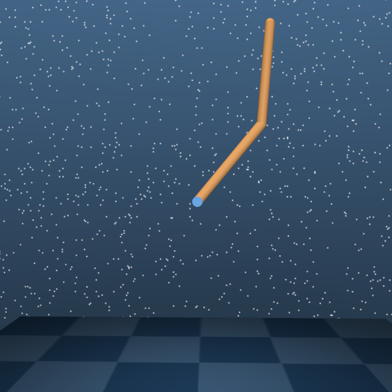
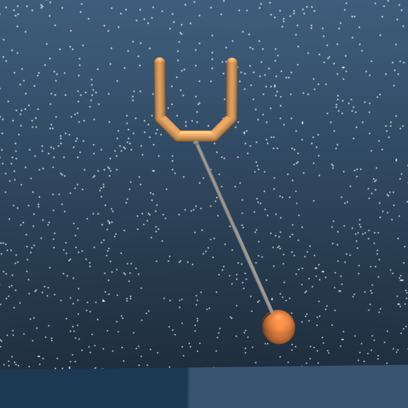
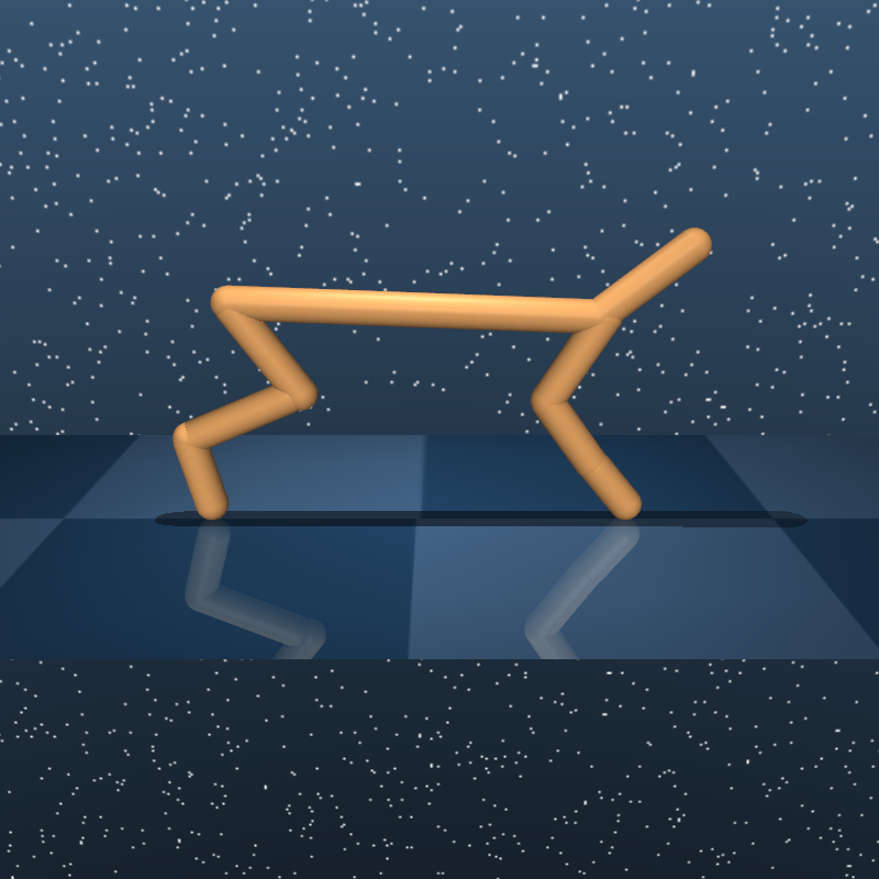
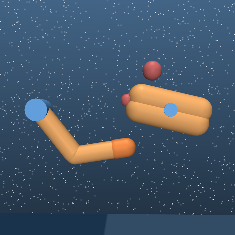
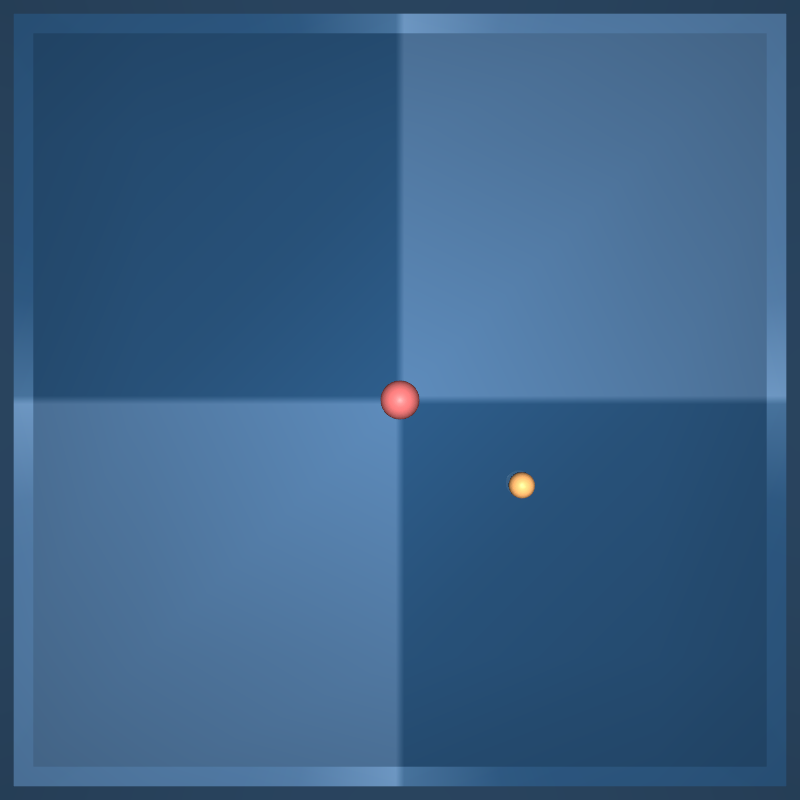
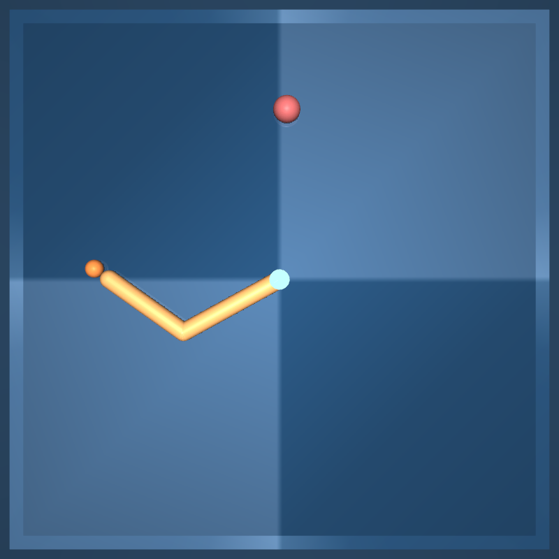
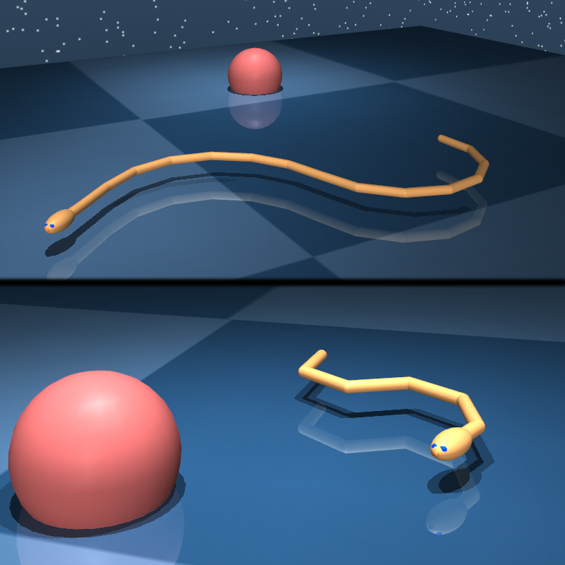
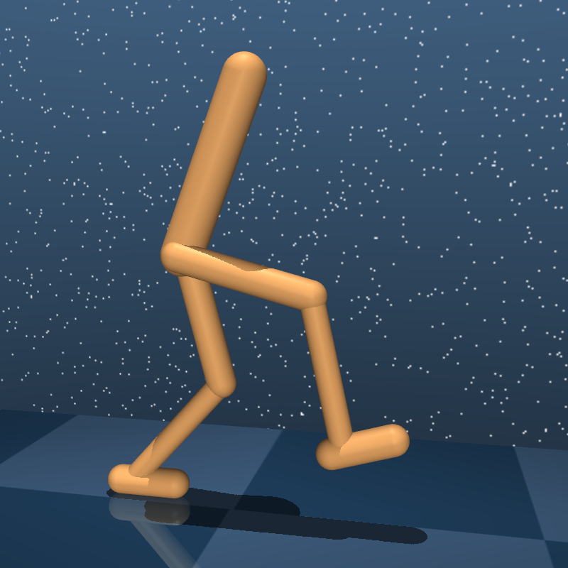
Figure 1: Benchmarking domains. Top: Acrobot, Ball-in-cup, Cart-pole, Cheetah, Finger, Fish, Hopper. Bottom: Humanoid, Manipulator, Pendulum, Point-mass, Reacher, Swimmer (6 and 15 links), Walker.

1 Introduction

Controlling the physical world is an integral part and arguably a prerequisite of general intelligence. Indeed, the only known example of general-purpose intelligence emerged in primates which had been manipulating the world for millions of years.

Physical control tasks share many common properties and it is sensible to consider them as a distinct class of behavioural problems. Unlike board games, language and other symbolic domains, physical tasks are fundamentally continuous in state, time and action. Their dynamics are subject to second-order equations of motion, implying that the underlying state is composed of position-like and velocity-like variables, while state derivatives are acceleration-like. Sensory signals (i.e. observations) usually carry meaningful physical units and vary over corresponding timescales.

This decade has seen rapid progress in the application of Reinforcement Learning (RL) techniques to difficult problem domains such as video games (Mnih, 2015). The Arcade Learning Environment (ALE, Bellemare et al. 2012) was a vital facilitator of these developments, providing a set of standard benchmarks for evaluating and comparing learning algorithms. The DeepMind Control Suite provides a similar set of standard benchmarks for continuous control problems.

The OpenAI Gym (Brockman et al., 2016) currently includes a set of continuous control domains that has become the de-facto benchmark in continuous RL (Duan et al., 2016; Henderson et al., 2017). The Control Suite is also a set of tasks for benchmarking continuous RL algorithms, with a few notable differences. We focus exclusively on continuous control, e.g. separating observations with similar units (position, velocity, force etc.) rather than concatenating into one vector. Our unified reward structure (see below) offers interpretable learning curves and aggregated suite-wide performance measures. Furthermore, we emphasise high-quality well-documented code using uniform design patterns, offering a readable, transparent and easily extensible codebase. Finally, the Control Suite has equivalent domains to all those in the Gym while adding many more¹¹1With the notable exception of Philipp Moritz’s “ant” quadruped, which we intend to replace soon, see Future Work..

In Section 2 we explain the general structure of the Control Suite and in Section 3 we describe each domain in detail. In Sections 4 and 5 we document the high and low-level Python APIs, respectively. Section 6 is devoted to our benchmarking results. We then conclude and provide a roadmap for future development.

2 Structure and Design

The DeepMind Control Suite is a set of stable, well-tested continuous control tasks that are easy to use and modify. Tasks are written in \hrefhttps://www.python.org/Python and physical models are defined using \hrefhttp://mujoco.org/book/modeling.htmlMJCF. Standardised action, observation and reward structures make benchmarking simple and learning curves easy to interpret.

Model and Task verification

Verification in this context means making sure that the physics simulation is stable and that the task is solvable:

•

Simulated physics can easily destabilise and diverge, mostly due to errors introduced by time discretisation. Smaller time-steps are more stable, but require more computation per unit simulation time, so the choice of time-step is always a trade-off between stability and speed (Erez et al., 2015). What’s more, learning agents are better at discovering and exploiting instabilities.²²2This phenomenon, sometimes known as Sims’ Law, was first articulated in (Sims, 1994): “Any bugs that allow energy leaks from non-conservation, or even round-off errors, will inevitably be discovered and exploited”.
•

It is surprisingly easy to write tasks that are much easier or harder than intended, that are impossible to solve or that can be solved by very different strategies than expected (i.e. “cheats”). To prevent these situations, the Atari™ games that make up ALE were extensively tested over more than 10 man-years³³3Marc Bellemare, personal communication.. However, continuous control domains cannot be solved by humans, so a different approach must be taken.

In order to tackle both of these challenges, we ran variety of learning agents (e.g. Lillicrap et al. 2015; Mnih et al. 2016) against all tasks, and iterated on each task’s design until we were satisfied that the physics was stable and non-exploitable, and that the task is solved correctly by at least one agent. Tasks that are solvable by some learning agent were collated into the benchmarking set. Tasks were not solved by any learning agent are in the extra set of tasks.

Reinforcement Learning

A continuous Markov Decision Process (MDP) is given by a set of states $\mathcal{S}$ , a set of actions $\mathcal{A}$ , a dynamics (transition) function $\mathbf{f}(\mathbf{s},\mathbf{a})$ , an observation function $\mathbf{o}(\mathbf{s},\mathbf{a})$ and a scalar reward function $r(\mathbf{s},\mathbf{a})$ .

State:: The state $\mathbf{s}$ is a vector of real numbers $\mathcal{S}\equiv\mathbb{R}^{\dim(\mathcal{S})}$ , with the exception of spatial orientations which are represented by unit quaternions $\in SU(2)$ . States are initialised in some subset $\mathcal{S}_{\textit{0}}\subseteq\mathcal{S}$ by the begin_episode() method. To avoid memorised “rote” solutions $\mathcal{S}_{\textit{0}}$ is never a single state.
Action:: With the exception of the LQR domain (see below), the action vector is in the unit box $\mathbf{a}\in\mathcal{A}\equiv\left[-1,1\right]^{\dim(\mathcal{A})}$ .
Dynamics:: While the state notionally evolves according to a continuous ordinary differential equation $\dot{\mathbf{s}}=\mathbf{f}_{c}(\mathbf{s},\mathbf{a})$ , in practice temporal integration is discrete⁴⁴4Most domains use MuJoCo’s default semi-implicit Euler integrator, a few which have smooth, nearly energy-conserving dynamics use 4th-order Runge Kutta. with some fixed, finite time-step: $\mathbf{s}_{t+h}=\mathbf{f}(\mathbf{s}_{t},\mathbf{a}_{t})$ .
Observation:: The function $\mathbf{o}(\mathbf{s},\mathbf{a})$ describes the observations available to the learning agent. With the exception of point-mass:hard (see below), all tasks are strongly observable, i.e. the state can be recovered from a single observation. Observation features which depend only on the state (position and velocity) are functions of the current state. Features which are also dependent on controls (e.g. touch sensor readings) are functions of the previous transition. Observations are implemented as a Python OrderedDict.
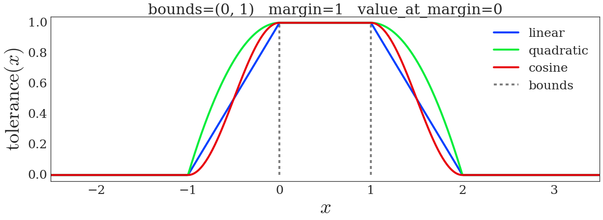
Reward:: The range of rewards in the Control Suite, with the exception of the LQR domain, are in the unit interval $r(\mathbf{s},\mathbf{a})\in[0,1]$ . Some tasks have “sparse” rewards $r(\mathbf{s},\mathbf{a})\in\{0,1\}$ . This structure is facilitated by the tolerance() function, see Figure 2. Since terms produced by tolerance() are in the unit interval, both averaging and multiplication operations maintain that property, facillitating cost design.
Termination and Discount:: Control problems are classified as finite-horizon, first-exit and infinite-horizon (Bertsekas, 1995). Control Suite tasks have no terminal states or time limit and are therefore of the infinite-horizon variety. Notionally the objective is the continuous-time infinite-horizon average return $\lim_{T\rightarrow\infty}T^{-1}\int_{0}^{T}r(\mathbf{s}_{t},\mathbf{a}_{t})dt$ , but in practice all of our agents internally use the discounted formulation $\int_{0}^{\infty}e^{-t/\tau}r(\mathbf{s}_{t},\mathbf{a}_{t})dt$ or, in discrete time $\sum_{i=0}^{\infty}\gamma^{i}r(\mathbf{s}_{i},\mathbf{a}_{i})$ , where $\gamma=e^{-h/\tau}$ is the discount factor. In the limit $\tau\rightarrow\infty$ (equivalently $\gamma\rightarrow 1$ ), the policies of the discounted-horizon and average-return formulations are identical.
Evaluation:: While agents are expected to optimise for infinite-horizon returns, these are difficult to measure. As a proxy we use fixed-length episodes of 1000 time steps. Since all reward functions are designed so that $r\approx 1$ at or near a goal state, learning curves measuring total returns all have the same y-axis limits of $\mathbf{[0,1000]}$ , making them easier to interpret.

Refer to caption — Figure 2: The tolerance(x, bounds=(lower, upper)) function will return 1 if x is within the bounds interval and 0 otherwise. If the optional margin argument is given, the output will decrease smoothly with distance from the interval, taking a value of value_at_margin at a distance of margin. Several types of sigmoid-like functions are available. Top: Three infinite-support sigmoids, for which value_at_margin must be positive. Bottom: Three finite-support support sigmoids with value_at_margin=0.

MuJoCo physics

MuJoCo (Todorov et al., 2012) is a fast, minimal-coordinate, continuous-time physics engine. It compares favourably to other popular engines (Erez et al., 2015), especially for articulated, low-to-medium degree-of-freedom (DoF) models in contact with other bodies. The convenient \hrefhttp://mujoco.org/book/modeling.htmlMJCF definition format and reconfigurable computation pipeline have made MuJoCo popular⁵⁵5Along with the MultiBody branch of the \hrefhttp://bulletphysics.org/wordpress/Bullet physics engine. for robotics and reinforcement learning research (e.g. Schulman et al. 2015).

3 Domains and Tasks

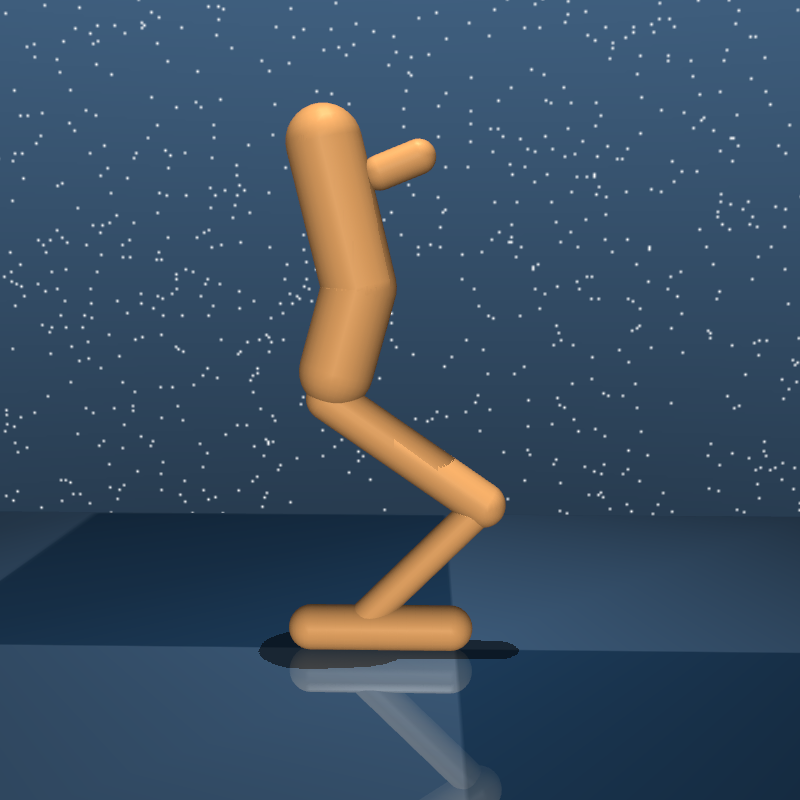
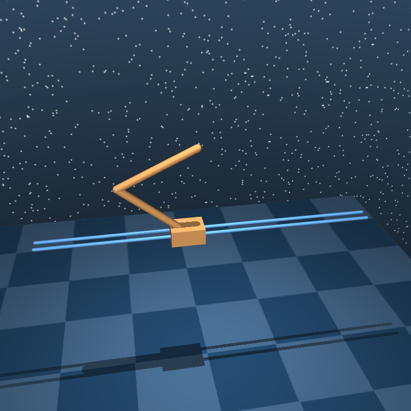
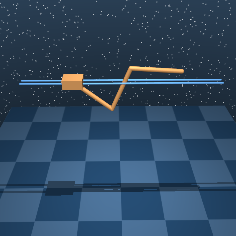
A domain refers to a physical model, while a task refers to an instance of that model with a particular MDP structure. For example the difference between the swingup and balance tasks of the cartpole domain is whether the pole is initialised pointing downwards or upwards, respectively. In some cases, e.g. when the model is procedurally generated, different tasks might have different physical properties. Tasks in the Control Suite are collated into tuples according predefined tags. In particular, tasks used for benchmarking are in the BENCHMARKING tuple, while those not used for benchmarking (because they are particularly difficult, or because they don’t conform to the standard structure) are in the EXTRA tuple. All suite tasks are accessible via the ALL_TASKS tuple. In the domain descriptions below, names are followed by three integers specifying the dimensions of the state, control and observation spaces i.e. $\Bigl{(}\dim(\mathcal{S}),\dim(\mathcal{A}),\dim(\mathcal{O})\Bigr{)}$ .

CMU Motion Capture Data

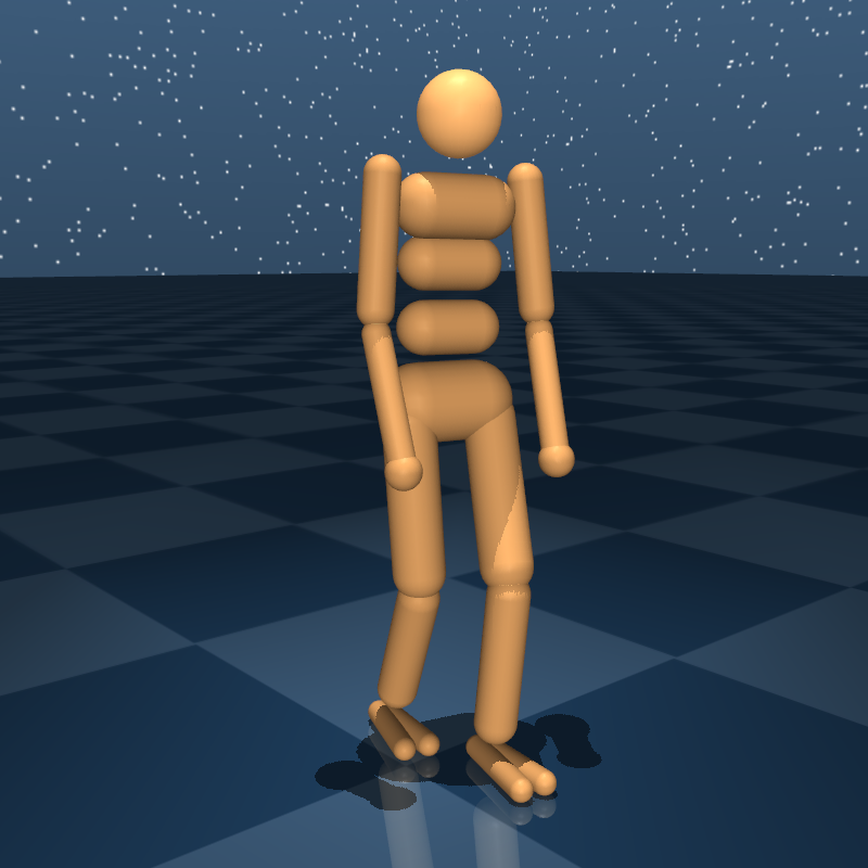
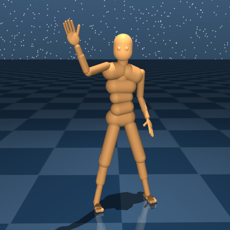
We enable humanoid_CMU to be used for imitation learning as in Merel et al. (2017) by providing tools for parsing, conversion and playback of human motion capture data from the CMU Motion Capture Database. The convert() function in the parse_amc module loads an AMC data file and returns a sequence of configurations for the humanoid_CMU model. The example script CMU_mocap_demo.py uses this function to generate a video.

4 Reinforcement learning API

In this section we describe the following Python code:

•

The environment.Base class that defines generic RL interface.
•

The suite module that contains the domains and tasks defined in Section 3
•

The underlying MuJoCo bindings and the mujoco.Physics class that provides most of the functionality needed to interact with an instantiated MJCF model.

The RL Environment class

The class environment.Base, found within the dm_control.rl.environment module, defines the following abstract methods:

$\bullet$ action_spec() and observation_spec(): describe the actions accepted and the observations returned by an Environment. For all the tasks in the suite, actions are given as a single NumPy array. action_spec() returns an ArraySpec, with attributes describing the shape, data type, and optional minimum and maximum bounds for the action arrays. Observations consist of an OrderedDict containing one or more NumPy arrays. observation_spec() returns an OrderedDict of ArraySpecs describing the shape and data type of each corresponding observation.
$\bullet$ reset() and step(): respectively start a new episode, and advance time given an action.

Starting an episode and running it to completion might look like

⬇

spec = env.action_spec()

time_step = env.reset()

while not time_step.last():

action = np.random.uniform(spec.minimum, spec.maximum, spec.shape)

time_step = env.step(action)

Both reset() and step() return a TimeStep namedtuple with fields [step_type, reward, discount, observation]:

$\bullet$ step_type: is an enum taking a value in [FIRST, MID, LAST]. The convenience methods first(), mid() and last() return boolean values indicating whether the TimeStep’s type is of the respective value.
$\bullet$ reward: is a scalar float.
$\bullet$ discount: is a scalar float $\gamma\in[0,1]$ .
$\bullet$ observation: is an OrderedDict of NumPy arrays matching the specification returned by observation_spec().

Whereas the step_type specifies whether or not the episode is terminating, it is the discount $\gamma$ that determines the termination type. $\gamma=0$ corresponds to a terminal state⁶⁶6i.e. where the sum of future reward is equal to the current reward. as in the first-exit or finite-horizon formulations. A terminal TimeStep with $\gamma=1$ corresponds to the infinite-horizon formulation. In this case an agent interacting with the environment should treat the episode as if it could have continued indefinitely, even though the sequence of observations and rewards is truncated. All Control Suite tasks with the exception of LQR⁷⁷7The LQR task terminates with $\gamma=0$ when the state is very close to 0, which is a proxy for the infinite exponential convergence of stabilised linear systems. return $\gamma=1$ at every step, including on termination.

The suite module

To load an environment representing a task from the suite, use suite.load():

⬇

from dm_control import suite

# Load one task:

env = suite.load(domain_name="cartpole", task_name="swingup")

# Iterate over a task set:

for domain_name, task_name in suite.BENCHMARKING:

env = suite.load(domain_name, task_name)

...

Wrappers can be used to modify the behaviour of control environments:

: Pixel observations

By default, Control Suite environments return low-dimensional feature observations. The pixel.Wrapper adds or replaces these with images.

⬇

from dm_control.suite.wrappers import pixels

env = suite.load("cartpole", "swingup")

env_and_pixels = pixels.Wrapper(env)

# Replace existing features by pixel observations.

env_only_pixels = pixels.Wrapper(env, pixel_only=False)

# Pixel observations in addition to existing features.
: Reward visualisation

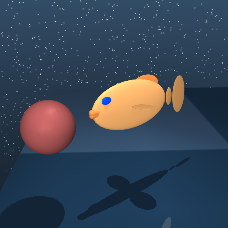
Models in the Control Suite use a common set of colours and textures for visual uniformity. As illustrated in the \hrefhttps://youtu.be/rAai4QzcYbsvideo, this also allows us to modify colours in proportion to the reward, providing a convenient visual cue.

⬇

env = suite.load("fish", "swim", task_kwargs, visualize_reward=True)

5 MuJoCo Python interface

While the environment.Base class is specific to the Reinforcement Learning scenario, the underlying bindings and mujoco.Physics class provide a general-purpose wrapper of the MuJoCo engine. We use Python’s \hrefhttps://docs.python.org/3/library/ctypes.htmlctypes library to bind to MuJoCo structs, enums and functions.

: Functions

The bindings provide easy access to all MuJoCo library functions, automatically converting NumPy arrays to data pointers where appropriate.

⬇

from dm_control.mujoco.wrapper.mjbindings import mjlib

import numpy as np

quat = np.array((.5, .5, .5, .5))

mat = np.zeros((9))

mjlib.mju_quat2Mat(mat, quat)

print("MuJoCo can convert this quaternion:")

print(quat)

print("To this rotation matrix:")

print(mat.reshape(3,3))

⬇

MuJoCo can convert this quaternion:

[ 0.5 0.5 0.5 0.5]

To this rotation matrix:

[[ 0. 0. 1.]

[ 1. 0. 0.]

[ 0. 1. 0.]]
: Enums

⬇

from dm_control.mujoco.wrapper.mjbindings import enums

print(enums.mjtJoint)

⬇

mjtJoint(mjJNT_FREE=0, mjJNT_BALL=1, mjJNT_SLIDE=2, mjJNT_HINGE=3)

The Physics class

The Physics class encapsulates MuJoCo’s most commonly used functionality.

: Loading an MJCF model

The Physics.from_xml_string() method loads an MJCF model and returns a Physics instance:

⬇

simple_MJCF = """

<mujoco>

<worldbody>

<light name="top" pos="0 0 1.5"/>

<geom name="floor" type="plane" size="1 1 .1"/>

<body name="box" pos="0 0 .3">

<joint name="up_down" type="slide" axis="0 0 1"/>

<geom name="box" type="box" size=".2 .2 .2" rgba="1 0 0 1"/>

<geom name="sphere" pos=".2 .2 .2" size=".1" rgba="0 1 0 1"/>

</body>

</worldbody>

</mujoco>

"""

physics = mujoco.Physics.from_xml_string(simple_MJCF)
: Rendering

The Physics.render() method outputs a numpy array of pixel values.

⬇

pixels = physics.render()

Optional arguments to render can be used to specify the resolution, camera ID and whether to render RGB or depth images.
: Physics.model and Physics.data

MuJoCo’s mjModel and mjData structs, describing static and dynamic simulation parameters, can be accessed via the model and data properties of Physics. They contain NumPy arrays that have direct, writeable views onto MuJoCo’s internal memory. Because the memory is owned by MuJoCo an attempt to overwrite an entire array will fail:

⬇

# This will fail:

physics.data.qpos = np.random.randn(physics.model.nq)

# This will succeed:

physics.data.qpos[:] = np.random.randn(physics.model.nq)
: Setting the state with reset_context()

When setting the MujoCo state, derived quantities like global positions or sensor measurements are not updated. In order to facilitate synchronisation of derived quantities we provide the Physics.reset_context() context:

⬇

with physics.reset_context():

# mj_reset() is called upon entering the context.

physics.data.qpos[:] = ... # Set position,

physics.data.qvel[:] = ... # velocity

physics.data.ctrl[:] = ... # and control.

# mj_forward() is called upon exiting the context. Now all derived

# quantities and sensor measurements are up-to-date.
: Running the simulation

The physics.step() method is used to advance the simulation. Note that this method does not directly call MuJoCo’s mj_step() function. At the end of an mj_step the state is updated, but the intermediate quantities stored in mjData were computed with respect to the previous state. To keep these derived quantities as closely synchronised with the current simulation state as possible, we use the fact that MuJoCo partitions mj_step into two parts: mj_step1, which depends only on the state and mj_step2, which also depends on the control. Our physics.step first executes mj_step2 (assuming mj_step1 has already been called), and then calls mj_step1, beginning the next step⁸⁸8In the case of Runge-Kutta integration, we simply conclude each RK4 step with an mj_step1.. The upshot is that quantities that depend only on position and velocity (e.g. camera pixels) are synchronised with the current state, while quantities that depend on force/acceleration (e.g. touch sensors) are with respect to the previous transition.
: Named indexing

It is often more convenient and less error-prone to refer to elements in the simulation by name rather than by index. Physics.named.model and Physics.named.data provide array-like containers that provide convenient named views:

⬇

print("The geom_xpos array:")

print(physics.data.geom_xpos)

print("Is much easier to inspect using Physics.named")

print(physics.named.data.geom_xpos)

⬇

The data.geom_xpos array:

[[ 0. 0. 0. ]

[ 0. 0. 0.3]

[ 0.2 0.2 0.5]]

Is much easier to inspect using Physics.named:

x y z

0 floor [ 0 0 0 ]

1 box [ 0 0 0.3 ]

2 sphere [ 0.2 0.2 0.5 ]

These containers can be indexed by name for both reading and writing, and support most forms of NumPy indexing:

⬇

with physics.reset_context():

physics.named.data.qpos["up_down"] = 0.1

print(physics.named.data.geom_xpos["box", ["x", "z"]])

⬇

[ 0. 0.4]

Note that in the example above we use a joint name to index into the generalised position array qpos. Indexing into a multi-DoF ball or free joint would output the appropriate slice.

We also provide convenient access to MuJoCo’s mj_id2name and mj_name2id:

⬇

physics.model.id2name(0, "geom")

⬇

'floor'

6 Benchmarking

We provide baselines for two commonly employed deep reinforcement learning algorithms A3C (Williams and Peng, 1991; Mnih et al., 2016) and DDPG (Lillicrap et al., 2015), as well as the recently introduced D4PG (Anonymous, 2017b). We refer to the relevant papers for algorithm motivation and details and here provide only hyperparameter, network architecture, and training configuration information (see relevant sections below).

We study both the case of learning with state derived features as observations and learning from raw-pixel inputs for all the tasks in the Control Suite. It is of course possible to look at control via combined state features and pixel features, but we do not study this case here. We present results for both final performance and learning curves that demonstrate aspects of data-efficiency and stability of training.

Establishing baselines for reinforcement learning problems and algorithms is notoriously difficult (Islam et al., 2017; Henderson et al., 2017). Though we describe results for well-functioning implementations of the algorithms we present, it may be possible to perform better on these tasks with the same algorithms. For a given algorithm we ran experiments with a similar network architecture, set of hyperparameters, and training configuration as described in the original papers. We ran a simple grid search for each algorithm to find a well performing setting for each (see details for grid searches below). We used the same hyperparameters across all of the tasks (i.e. so that nothing is tuned per-task). Thus, it should be possible to improve performance on a given task by tuning parameters with respect to performance for that specific task. For these reasons, the results are not presented as upper bounds for performance with these algorithms, but rather as a starting point for comparison. It is also worth noting that we have not made a concerted effort to maximise data efficiency, for example by making many mini-batch updates using the replay buffer per step in the environment, as in Popov et al. (2017).

The following pseudocode block demonstrates how to load a single task in the benchmark suite, run a single episode with a random agent, and compute the reward as we do for the results reported here. Note that we run each environment for 1000 time steps and sum the rewards provided by the environment after each call to step. Thus, the maximum possible score for any task is 1000. For many tasks, the practical maximum is significantly less than 1000 since it may take many steps until it’s possible to drive the system into a state that gives a full reward of 1.0 each time step.

⬇

from dm_control import suite

env = suite.load(domain_name, task_name)

spec = env.action_spec()

time_step = env.reset()

total_reward = 0.0

for _ in range(1000):

action = np.random.uniform(spec.minimum, spec.maximum, spec.shape)

time_step = env.step(action)

total_reward += time_step.reward

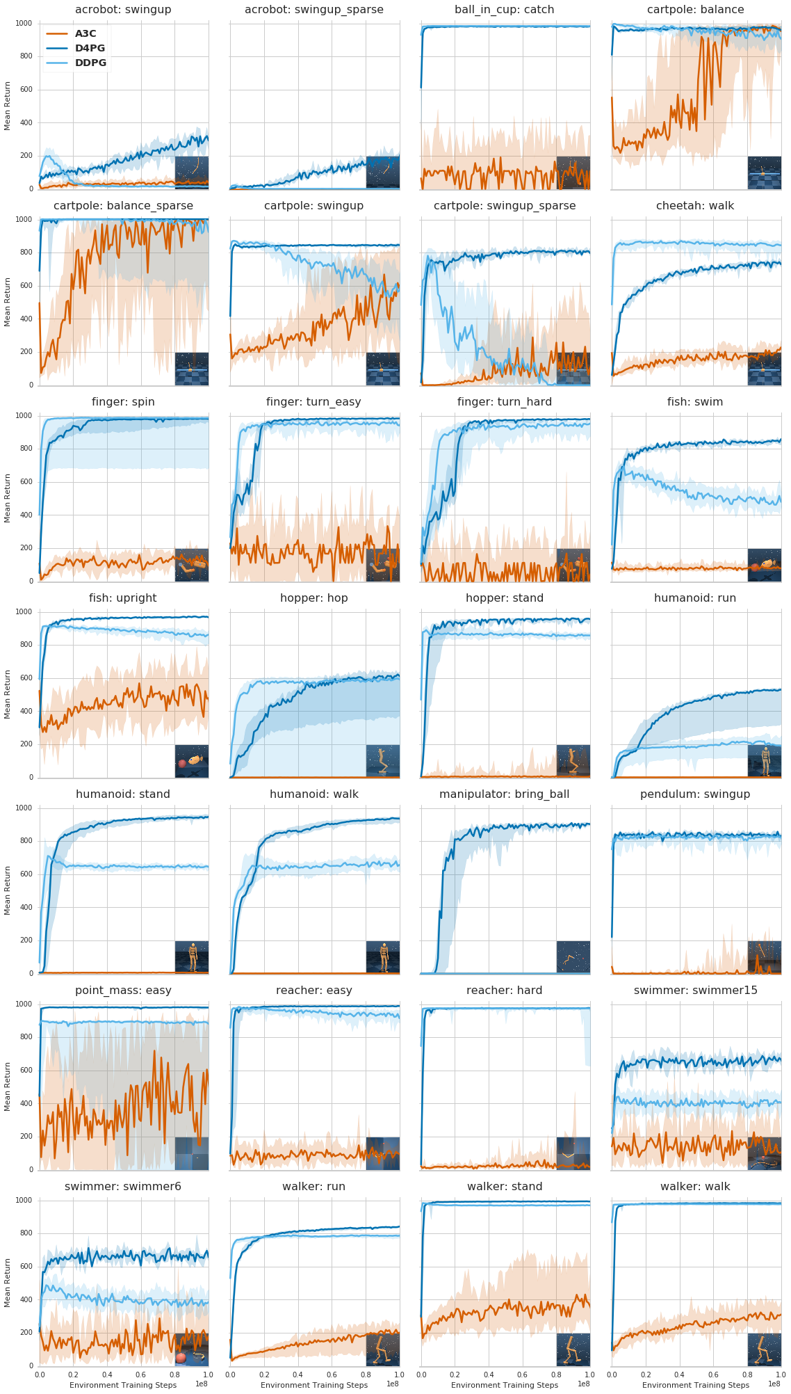
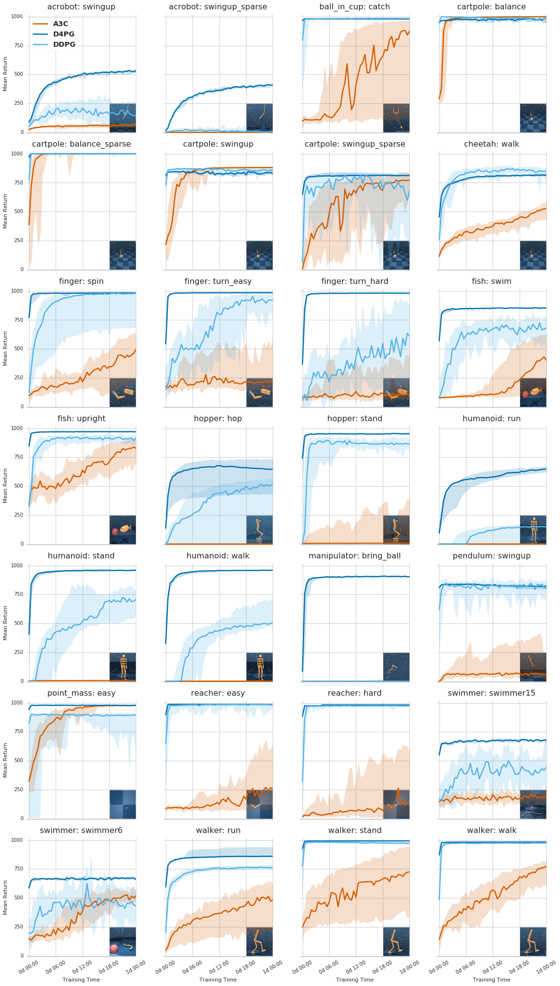
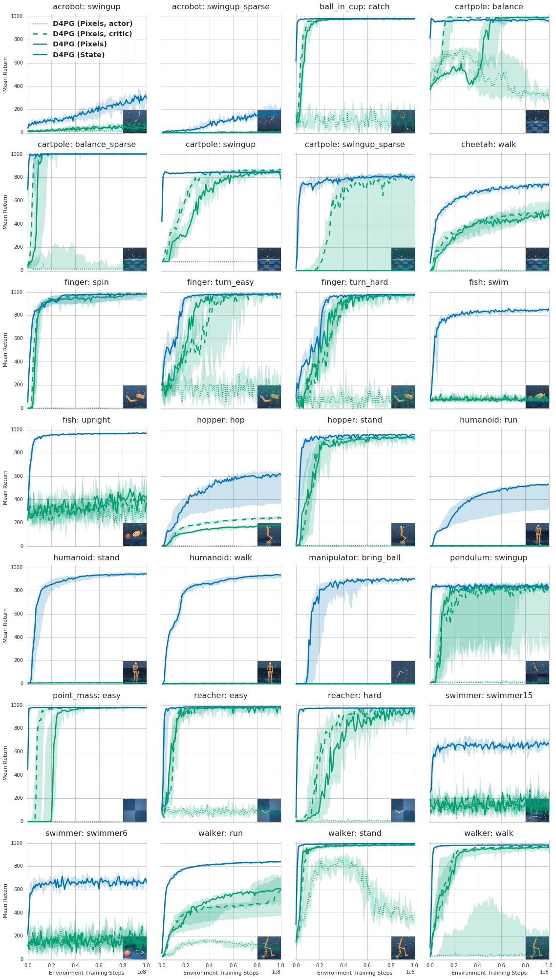
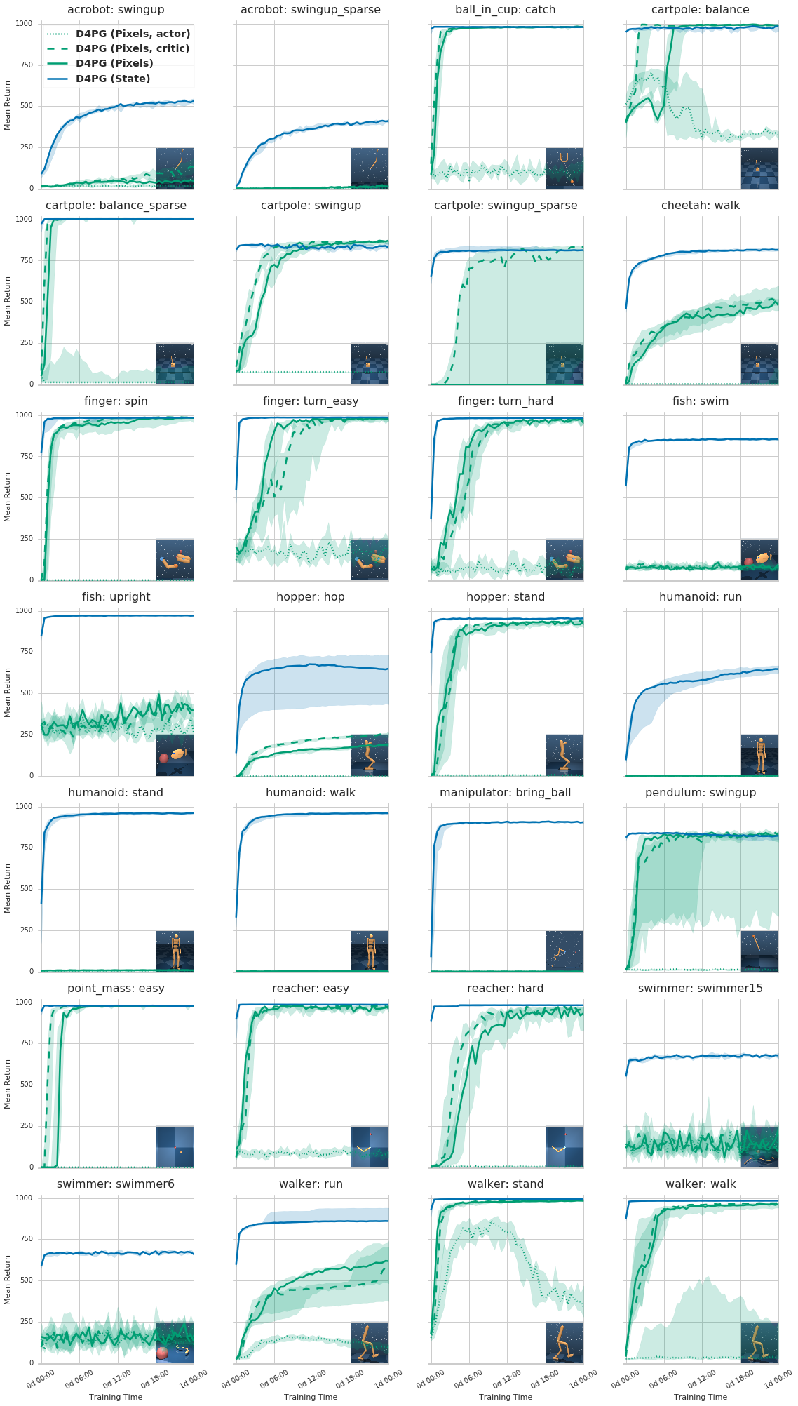
In the state feature case we ran 15 different seeds for each task with A3C and DDPG; for results with D4PG, which was generally found to be more stable, we ran 5 seeds. In the raw-pixel case we also ran 5 different seeds for each task. The seed sets the network weight initialisation for the associated run. In all cases, initial network weights were sampled using standard TensorFlow initialisers. In the figures showing performance on individual tasks (Figures 4-7), the lines denote the median performance and the shaded regions denote the 5^th and 95^th percentiles across seeds. In the tables showing performance for individual tasks (Tables 1 & 2) we report means and standard errors across seeds.

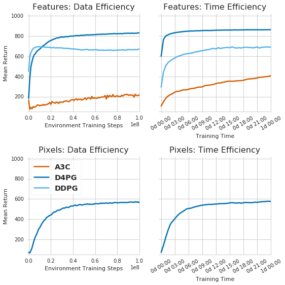
As well as studying performance on individual tasks, we examined the performance of algorithms across all tasks by plotting a simple aggregate measure. Figure 3 shows the mean performance over environment steps and wallclock time for both state features and raw-pixels. These measures are of particular interest: they offer a view into the generality of a reinforcement learning algorithm. In this aggregate view, it is clear that D4PG is the best performing agent in all metrics, with the exception that DDPG is more data efficient before $1\mathrm{e}{7}$ environment steps. It is worth noting that the data efficiency for D4PG can be improved over DDPG by simply reducing the number of actor threads for D4PG (experiments not shown here), since with 32 actors D4PG is somewhat wasteful of environment data (with the benefit of being more efficient in terms of wall-clock).

While we have made a concerted effort to ensure reproducible benchmarks, it’s worth noting that there remain uncontrolled aspects that introduce variance into the evaluations. For example, some tasks have a randomly placed target or initialisation of the model, and the sequence of these are not fixed across runs. Thus, each learning run will see a different sequence of episodes, which will lead to variance in performance. This might be fixed by introducing a fixed sequence of initialisation for episodes, but this is not in any case a practical solution for the common case of parallelised training, so our benchmarks simply reflect variability in episode initialisation sequence.

Algorithm and Architecture Details

A3C: Mnih et al. (2016) proposed a version of the Advantage Actor Critic (A2C; Williams and Peng 1991) that could be trained asynchronously (A3C). Here we report results for the A3C trained with 32 workers per task. The network consisted of 2 MLP layers shared between actor and critic with 256 units in the first hidden layer. The grid search explored: learning rates, $\eta\in$ [1e-2, 1e-3, 1e-4, 1e-5, 3e-5, 4e-5, 5e-5]; unroll length $t_{\mathrm{max}}\in[20,100,1000]$ ; activation functions for computing $\log\sigma(\cdot)\in[\mathrm{Softplus}(x),\exp(\log(0.01+2\text{sigmoid}(x)))]$ ; number of units in the second hidden layer $\in[128,256]$ ; annealing of learning rate $\in[\mathrm{true},\mathrm{false}]$ . The advantage baseline was computed using a linear layer after the second hidden layer. Actions were sampled from a multivariate Gaussian with diagonal covariance, parameterized by the output vectors $\mathbf{\mu}$ and $\mathbf{\sigma}^{2}$ . The value of the logarithm of $\mathbf{\sigma}$ was computed using the second sigmoid activation function given above (which was found to be more stable than the $\mathrm{Softplus}(x)$ function used in the original A3C manuscript), while $\mathbf{\mu}$ was computed from a hyperbolic tangent, both stemming from the second MLP layer. The RMSProp optimiser was used with a decay factor of $\alpha=0.99$ , a damping factor of $\epsilon=0.1$ and a learning rate starting at $5\mathrm{e}{-5}$ and annealed to $0$ throughout training using a linear schedule, with no gradient clipping. An entropy regularisation cost weighted at $\beta=3\mathrm{e}{-3}$ was added to the policy loss.
DDPG: Lillicrap et al. (2015) presented a Deep Deterministic Policy Gradients (DDPG) agent that performed well on an early version of the Control Suite. Here we present performance for straightforward single actor/learner implementation of the DDPG algorithm. Both actor and critic networks were MLPs with ReLU nonlinearities. The actor network had two layers of $300\rightarrow 200$ units respectively, while the critic network had two layers of $400\rightarrow 300$ units. The action vector was passed through a linear layer and summed up with the activations of the second critic layer in order to compute Q values. The grid search explored: discount factors, $\lambda\in[0.95,0.99]$ ; learning rates, $\eta\in[1\mathrm{e}{-2},1\mathrm{e}{-3},1\mathrm{e}{-4},1\mathrm{e}{-5}]$ fixed to be the same for both networks; damping and spread parameters for the Ornstein–Uhlenbeck process, $\theta\in[0,0.15,0.85,1]$ and $\mu\in[0.1,0.2,0.3,0.4]$ respectively; hard (swap at intervals of 100 steps) versus soft ( $\tau=1\mathrm{e}{-3}$ ) target updates. For the results shown here the two networks were trained with independent Adam optimisers Kingma and Ba (2014), both with a learning rate of $\eta=1\mathrm{e}{-4}$ , with gradients clipped at $[-1,1]$ for the actor network. The agent used discounting of $\lambda=0.99$ . As in the paper, we used a target network with soft updates and an Ohrstein-Uhlenbeck process to add an exploration noise that is correlated in time, with similar parameters, except for a slightly bigger $\sigma$ ( $\theta=0.15$ , $\sigma=0.3$ , $\tau=1\mathrm{e}{-3}$ ). The replay buffer size was also kept to $1\mathrm{e}6$ , and training was done with a minibatch size of $64$ .
D4PG: The Distributional Distributed Deep Deterministic Policy Gradients algorithm (Anonymous, 2017b) extends regular DDPG with the following features: First, the critic value function is modelled as a categorical distribution (Bellemare et al., 2017), using 101 categories spaced evenly across $[-150,150]$ . Second, acting and learning are decoupled and deployed on separate machines using the Ape-X architecture described in (Anonymous, 2017a). We used 32 CPU-based actors and a single GPU-based learner for benchmarking. D4PG additionally applies $N$ -step returns with $N=5$ , and non-uniform replay sampling (Schaul et al., 2015) ( $\alpha_{\text{sample}}=0.6$ ) and eviction ( $\alpha_{\text{evict}}=0.6$ ) strategies using a sample-based distributional KL loss (see (Anonymous, 2017a) and (Anonymous, 2017b) for details). D4PG hyperparameters were the same as those used for DDPG, with the exception that (1) hard target network updates are applied every 100 steps, and (2) exploration noise is sampled from a Gaussian distribution with fixed $\sigma$ varying from $1/32$ to $1$ across the actors. A mini-batch size of $256$ was used.

Results: Learning from state features

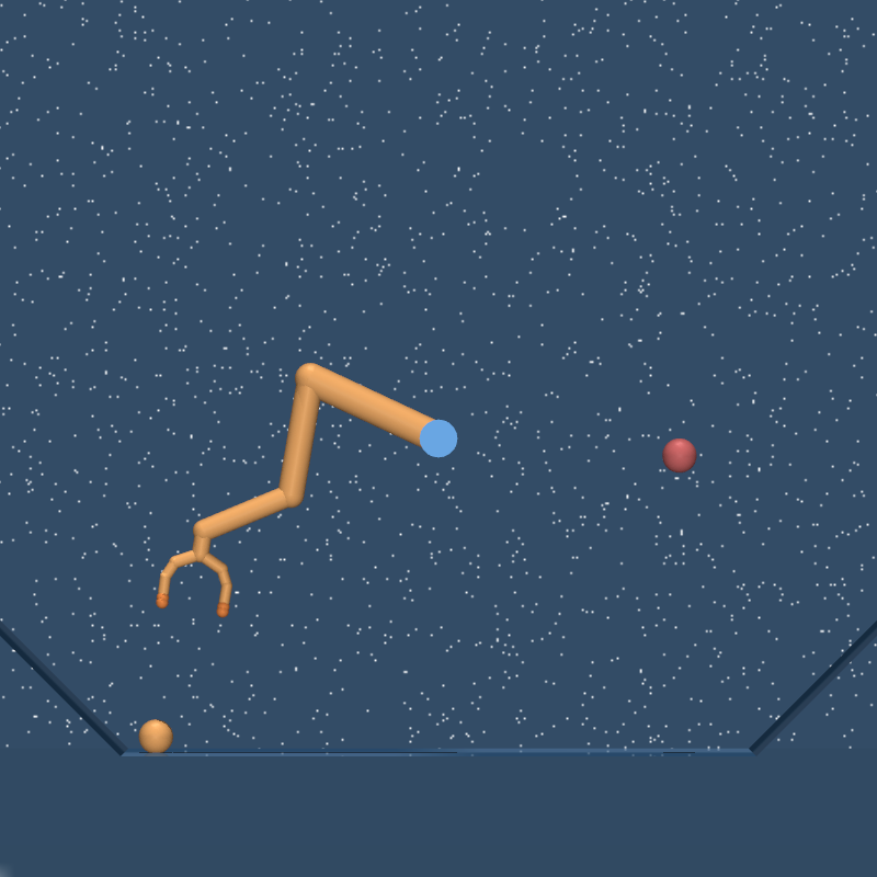
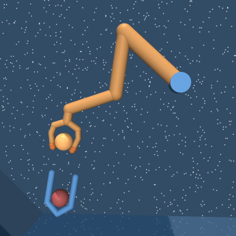
Due to the different parallelization architectures, the evaluation protocol for each agent was slightly different: DDPG was evaluated for 10 episodes for every 100000 steps (with no exploration noise), and A3C was trained with 32 workers and concurrently evaluated with another worker that updated its parameters every 3 episodes, which produced intervals of on average 96000 steps per update. The plots in Figure 4 and Figure 5 show the median and the 5th and 95th percentile of the returns for the first $1\mathrm{e}8$ steps. Each agent was run 15 times per task using different seeds (except for D4PG which was run 5 times), using only low-dimensional state feature information. D4PG tends to achieve better results in nearly all of the tasks. Notably, it manages to reliably solve the manipulator:bring_ball task, and achieves a good performance in acrobot tasks. We found that part of the reason the agent did not go above $600$ in the acrobot task is due to the time it takes for the pendulum to be swung up, so its performance is probably close to the upper bound.

Results: Learning from pixels

The DeepMind Control Suite can be configured to produce observations containing any combination of state vectors and pixels generated from the provided cameras. We also benchmarked a variant of D4PG that learns directly from pixel-only input, using $84\times 84$ RGB frames from the $0^{\mathrm{th}}$ camera. To process pixel input, D4PG is augmented with a simple 2-layer ConvNet. Both kernels are size $3\times 3$ with 32 channels and ELU activation, and the first layer has stride 2. The output is fed through a single fully-connected layer with 50 neurons, with layer normalisation Ba et al. (2016) and tanh() activations. We explored four variants of the algorithm. In the first, there were separate networks for the actor and Q-critic. In the other three, the actor and critic shared the convolutional layers, and the actor and critic each had a separate fully connected layer before their respective outputs. The best performance was obtained by weight-sharing the convolutional kernel weights between the actor and critic networks, and only allowing these weights to be updated by the critic optimiser (i.e. truncating the policy gradients after the actor MLP). D4Pixels internally frame-stacks 3 consecutive observations as the ConvNet input.

Results for 1 day of running time are shown in Figure 7; we plot the results for the three shared-weights variants of D4PG, with gradients into the ConvNet from the actor (dotted green), critic (dashed green), or both (solid green). For the sake of comparison, we plot D4PG performance for low-dimensional features (solid blue) from Figure 5. The variant that employed separate networks for actor and critic performed significantly worse than the best of these and is not shown. Learning from pixel-only input is successful on many of the tasks, but fails completely in some cases. It is worth noting that the camera view for some of the task domains are not well suited to a pixel-only solution for the task. Thus, some of the failure cases are likely due to the difficulty of positioning a camera that simultaneously captures both the navigation targets as well as the details of the agents body: e.g., in the case of swimmer:swimmer6 and swimmer15 as well as fish:swim.

7 Conclusion and future work

The DeepMind Control Suite is a starting place for the design and performance comparison of reinforcement learning algorithms for physics-based control. It offers a wide range of tasks, from near-trivial to quite difficult. The uniform reward structure allows for robust suite-wide performance measures.

The results presented here for A3C, DDPG, and D4PG constitute baselines using, to the best of our knowledge, well performing implementations of these algorithms. At the same time, we emphasise that the learning curves are not based on exhaustive hyperparameter optimisation, and that for a given algorithm the same hyperparameters were used across all tasks in the Control Suite. Thus, we expect that it may be possible to obtain better performance or data efficiency, especially on a per-task basis.

We are excited to be sharing the Control Suite with the wider community and hope that it will be found useful. We look forward to the diverse research the Suite may enable, and to integrating community contributions in future releases.

Future work

Several elements are missing from the current release of the Control Suite.

Some features, like the lack of rich tasks, are missing by design. The Suite, and particularly the benchmarking set of tasks, is meant to be a stable, simple starting point for learning control. Task categories like full manipulation and locomotion in complex terrains require reasoning about a distribution of tasks and models, not only initial states. These require more powerful tools which we hope to share in the future in a different branch.

There are several features that we hoped to include but did not make it into this release; we intend to add these in the future. They include: a quadrupedal locomotion task, an interactive visualiser with which to view and perturb the simulation, support for C callbacks and multi-threaded dynamics, a MuJoCo TensorFlow op wrapper and Windows™ support.

A3C D4PG D4PG (Pixels) DDPG Domain Task acrobot swingup 41.9 ± 1.2 297.6 ± 8.4 81.7 ± 4.4 15.4 ± 0.9 swingup_sparse 0.2 ± 0.1 198.7 ± 9.1 13.0 ± 1.7 1.0 ± 0.1 ball_in_cup catch 104.7 ± 7.8 981.2 ± 0.7 980.5 ± 0.5 984.5 ± 0.3 cartpole balance 951.6 ± 2.4 966.9 ± 1.9 992.8 ± 0.3 917.4 ± 2.2 balance_sparse 857.4 ± 7.9 1000.0 ± 0.0 1000.0 ± 0.0 878.5 ± 8.0 swingup 558.4 ± 6.8 845.5 ± 1.2 862.0 ± 1.1 521.7 ± 6.1 swingup_sparse 179.8 ± 5.9 808.4 ± 4.4 482.0 ± 56.6 4.5 ± 1.1 cheetah walk 213.9 ± 1.6 736.7 ± 4.4 523.8 ± 6.8 842.5 ± 1.6 finger spin 129.4 ± 1.5 978.2 ± 1.5 985.7 ± 0.6 920.3 ± 6.3 turn_easy 167.3 ± 9.6 983.4 ± 0.6 971.4 ± 3.5 942.9 ± 4.3 turn_hard 88.7 ± 7.3 974.4 ± 2.8 966.0 ± 3.4 939.4 ± 4.1 fish swim 81.3 ± 1.1 844.3 ± 3.1 72.2 ± 3.0 492.7 ± 9.8 upright 474.6 ± 6.6 967.4 ± 1.0 405.7 ± 19.6 854.8 ± 3.3 hopper hop 0.5 ± 0.0 560.4 ± 18.2 242.0 ± 2.1 501.4 ± 6.0 stand 27.9 ± 2.3 954.4 ± 2.7 929.9 ± 3.8 857.7 ± 2.2 humanoid run 1.0 ± 0.0 463.6 ± 13.8 1.4 ± 0.0 167.9 ± 4.1 stand 6.0 ± 0.1 946.5 ± 1.8 8.6 ± 0.2 642.6 ± 2.1 walk 1.6 ± 0.0 931.4 ± 2.3 2.6 ± 0.1 654.2 ± 3.9 manipulator bring_ball 0.4 ± 0.0 895.9 ± 3.7 0.5 ± 0.1 0.6 ± 0.1 pendulum swingup 48.6 ± 5.2 836.2 ± 5.0 680.9 ± 41.9 816.2 ± 4.7 point_mass easy 545.3 ± 9.3 977.3 ± 0.6 977.8 ± 0.5 618.0 ± 11.4 reacher easy 95.6 ± 3.5 987.1 ± 0.3 967.4 ± 4.1 917.9 ± 6.2 hard 39.7 ± 2.9 973.0 ± 2.0 957.1 ± 5.4 904.3 ± 6.8 swimmer swimmer15 164.0 ± 7.3 658.4 ± 10.0 180.8 ± 11.9 421.8 ± 13.5 swimmer6 177.8 ± 7.8 664.7 ± 11.1 194.7 ± 15.9 394.0 ± 14.1 walker run 191.8 ± 1.9 839.7 ± 0.7 567.2 ± 18.9 786.2 ± 0.4 stand 378.4 ± 3.5 993.1 ± 0.3 985.2 ± 0.4 969.8 ± 0.3 walk 311.0 ± 2.3 982.7 ± 0.3 968.3 ± 1.8 976.3 ± 0.3

Table 1: Mean and Standard Error of 100 episodes after

10^{8}

training steps for each seed.

A3C D4PG D4PG (Pixels) DDPG Domain Task acrobot swingup 64.7 ± 2.0 531.1 ± 8.9 141.5 ± 6.9 149.8 ± 4.2 swingup_sparse 0.3 ± 0.1 415.9 ± 9.5 16.3 ± 2.0 8.5 ± 0.8 ball_in_cup catch 643.3 ± 10.9 979.8 ± 0.7 980.5 ± 0.6 984.4 ± 0.3 cartpole balance 999.0 ± 0.0 982.7 ± 1.4 988.3 ± 0.6 980.2 ± 0.6 balance_sparse 999.7 ± 0.1 999.7 ± 0.2 1000.0 ± 0.0 998.4 ± 0.7 swingup 881.4 ± 0.1 836.1 ± 1.6 864.0 ± 1.0 855.6 ± 0.6 swingup_sparse 752.5 ± 3.6 814.6 ± 0.7 649.6 ± 46.9 591.1 ± 7.3 cheetah walk 519.7 ± 2.2 814.6 ± 4.0 524.7 ± 6.8 849.7 ± 1.7 finger spin 446.7 ± 4.2 984.7 ± 0.4 986.2 ± 0.4 916.1 ± 6.3 turn_easy 291.9 ± 11.3 986.1 ± 0.5 976.0 ± 1.7 927.8 ± 4.9 turn_hard 200.6 ± 9.6 983.2 ± 0.5 971.0 ± 2.9 618.7 ± 11.8 fish swim 395.7 ± 7.3 852.5 ± 2.7 76.8 ± 4.2 666.8 ± 6.8 upright 813.6 ± 4.4 971.1 ± 0.9 366.8 ± 18.3 915.3 ± 2.0 hopper hop 0.7 ± 0.1 613.2 ± 18.0 249.8 ± 2.1 435.2 ± 4.9 stand 82.6 ± 5.9 956.8 ± 3.9 930.0 ± 3.4 862.8 ± 2.8 humanoid run 1.0 ± 0.0 643.1 ± 3.1 1.5 ± 0.0 137.3 ± 1.3 stand 7.8 ± 0.1 959.1 ± 0.8 8.7 ± 0.2 687.9 ± 2.1 walk 1.7 ± 0.0 960.3 ± 0.5 2.7 ± 0.1 534.4 ± 2.1 manipulator bring_ball 0.6 ± 0.1 903.7 ± 3.9 0.6 ± 0.1 1.2 ± 0.4 pendulum swingup 98.8 ± 9.5 814.9 ± 5.8 705.7 ± 36.7 818.6 ± 4.3 point_mass easy 978.5 ± 0.1 978.2 ± 0.7 979.3 ± 0.3 862.3 ± 3.1 reacher easy 285.3 ± 8.9 984.9 ± 1.1 967.1 ± 4.4 969.8 ± 3.0 hard 247.5 ± 9.4 982.8 ± 0.4 958.0 ± 5.2 975.3 ± 0.5 swimmer swimmer15 196.8 ± 8.4 681.1 ± 9.3 146.0 ± 12.0 410.9 ± 10.5 swimmer6 526.4 ± 9.6 651.0 ± 10.0 168.9 ± 13.1 461.0 ± 10.6 walker run 448.4 ± 4.1 891.5 ± 5.6 566.1 ± 19.1 766.5 ± 0.4 stand 707.9 ± 6.5 994.0 ± 0.3 984.8 ± 0.4 973.7 ± 0.3 walk 744.2 ± 2.4 983.1 ± 0.4 968.1 ± 1.8 975.7 ± 0.3

Table 2: Mean and standard error of 100 episodes after 24 hours of training for each seed.

References

Anonymous (2017a) Anonymous. Distributed prioritized experience replay. Under submission, 2017a.
Anonymous (2017b) Anonymous. Distributional policy gradients. Under submission, 2017b.
Ba et al. (2016) Jimmy Lei Ba, Jamie Ryan Kiros, and Geoffrey E Hinton. Layer normalization. arXiv preprint arXiv:1607.06450, 2016.
Barto et al. (1983) A. G. Barto, R. S. Sutton, and C. W. Anderson. Neuronlike adaptive elements that can solve difficult learning control problems. IEEE Transactions on Systems, Man, and Cybernetics, SMC-13(5):834–846, Sept 1983. ISSN 0018-9472. doi: 10.1109/TSMC.1983.6313077.
Bellemare et al. (2012) Marc G Bellemare, Yavar Naddaf, Joel Veness, and Michael Bowling. The arcade learning environment: An evaluation platform for general agents. Journal of Artificial Intelligence Research, 2012.
Bellemare et al. (2017) Marc G Bellemare, Will Dabney, and Rémi Munos. A distributional perspective on reinforcement learning. arXiv preprint arXiv:1707.06887, 2017.
Bertsekas (1995) Dimitri P Bertsekas. Dynamic programming and optimal control, volume 1. Athena scientific Belmont, MA, 1995.
Brockman et al. (2016) Greg Brockman, Vicki Cheung, Ludwig Pettersson, Jonas Schneider, John Schulman, Jie Tang, and Wojciech Zaremba. Openai gym, 2016.
(9) CMU Graphics Lab. CMU Motion Capture Database. http://mocap.cs.cmu.edu, 2002. The database was created with funding from NSF EIA-0196217.
Coulom (2002) Rémi Coulom. Reinforcement learning using neural networks, with applications to motor control. PhD thesis, Institut National Polytechnique de Grenoble-INPG, 2002.
Duan et al. (2016) Yan Duan, Xi Chen, Rein Houthooft, John Schulman, and Pieter Abbeel. Benchmarking deep reinforcement learning for continuous control. In International Conference on Machine Learning, pages 1329–1338, 2016.
Erez et al. (2015) Tom Erez, Yuval Tassa, and Emanuel Todorov. Simulation tools for model-based robotics: Comparison of bullet, havok, mujoco, ode and physx. In Robotics and Automation (ICRA), 2015 IEEE International Conference on, pages 4397–4404. IEEE, 2015.
Henderson et al. (2017) Peter Henderson, Riashat Islam, Philip Bachman, Joelle Pineau, Doina Precup, and David Meger. Deep reinforcement learning that matters, 2017.
Islam et al. (2017) Riashat Islam, Peter Henderson, Maziar Gomrokchi, and Doina Precup. Reproducibility of benchmarked deep reinforcement learning tasks for continuous control. arXiv preprint arXiv:1708.04133, 2017.
Kingma and Ba (2014) Diederik Kingma and Jimmy Ba. Adam: A method for stochastic optimization. arXiv preprint arXiv:1412.6980, 2014.
Lillicrap et al. (2015) Timothy P Lillicrap, Jonathan J Hunt, Alexander Pritzel, Nicolas Heess, Tom Erez, Yuval Tassa, David Silver, and Daan Wierstra. Continuous control with deep reinforcement learning. arXiv preprint arXiv:1509.02971, 2015.
Merel et al. (2017) Josh Merel, Yuval Tassa, TB Dhruva, Sriram Srinivasan, Jay Lemmon, Ziyu Wang, Greg Wayne, and Nicolas Heess. Learning human behaviors from motion capture by adversarial imitation. arXiv preprint arXiv:1707.02201, 2017.
Mnih et al. (2016) Volodymyr Mnih, Adria Puigdomenech Badia, Mehdi Mirza, Alex Graves, Timothy P Lillicrap, Tim Harley, David Silver, and Koray Kavukcuoglu. Asynchronous methods for deep reinforcement learning. arXiv preprint arXiv:1602.01783, 2016.
Mnih (2015) Volodymyr et al. Mnih. Human-level control through deep reinforcement learning. Nature, 518(7540):529–533, Feb 2015. ISSN 0028-0836. Letter.
Popov et al. (2017) Ivaylo Popov, Nicolas Heess, Timothy Lillicrap, Roland Hafner, Gabriel Barth-Maron, Matej Vecerik, Thomas Lampe, Yuval Tassa, Tom Erez, and Martin Riedmiller. Data-efficient deep reinforcement learning for dexterous manipulation. arXiv preprint arXiv:1704.03073, 2017.
Schaul et al. (2015) Tom Schaul, John Quan, Ioannis Antonoglou, and David Silver. Prioritized experience replay. arXiv preprint arXiv:1511.05952, 2015.
Schulman et al. (2015) John Schulman, Sergey Levine, Pieter Abbeel, Michael Jordan, and Philipp Moritz. Trust region policy optimization. In Proceedings of the 32nd International Conference on Machine Learning (ICML-15), pages 1889–1897, 2015.
Sims (1994) Karl Sims. Evolving virtual creatures. In Proceedings of the 21st annual conference on Computer graphics and interactive techniques, pages 15–22. ACM, 1994.
Spong (1995) Mark W Spong. The swing up control problem for the acrobot. IEEE control systems, 15(1):49–55, 1995.
Tassa and Todorov (2010) Yuval Tassa and Emo Todorov. Stochastic complementarity for local control of discontinuous dynamics. In Proceedings of Robotics: Science and Systems (RSS, 2010.
Tassa et al. (2012) Yuval Tassa, Tom Erez, and Emanuel Todorov. Synthesis and stabilization of complex behaviors through online trajectory optimization. In Intelligent Robots and Systems (IROS), 2012 IEEE/RSJ International Conference on, pages 4906–4913. IEEE, 2012.
Todorov et al. (2012) Emanuel Todorov, Tom Erez, and Yuval Tassa. Mujoco: A physics engine for model-based control. In Intelligent Robots and Systems (IROS), 2012 IEEE/RSJ International Conference on, pages 5026–5033. IEEE, 2012.
Wawrzyński (2009) Paweł Wawrzyński. Real-time reinforcement learning by sequential actor–critics and experience replay. Neural Networks, 22(10):1484–1497, 2009.
Williams and Peng (1991) Ronald J Williams and Jing Peng. Function optimization using connectionist reinforcement learning algorithms. Connection Science, 3(3):241–268, 1991.