Sampling-Based Methods for Factored
Task and Motion Planning

Abstract

This paper presents a general-purpose formulation of a large class of discrete-time planning problems, with hybrid state and control-spaces, as factored transition systems. Factoring allows state transitions to be described as the intersection of several constraints each affecting a subset of the state and control variables. Robotic manipulation problems with many movable objects involve constraints that only affect several variables at a time and therefore exhibit large amounts of factoring. We develop a theoretical framework for solving factored transition systems with sampling-based algorithms. The framework characterizes conditions on the submanifold in which solutions lie, leading to a characterization of robust feasibility that incorporates dimensionality-reducing constraints. It then connects those conditions to corresponding conditional samplers that can be composed to produce values on this submanifold. We present two domain-independent, probabilistically complete planning algorithms that take, as input, a set of conditional samplers. We demonstrate the empirical efficiency of these algorithms on a set of challenging task and motion planning problems involving picking, placing, and pushing.

inline, color=blue!10, linecolor=blue!90, size=]TODO: It would be nice to highlight the ease of specification or something.

1 Introduction

Many important robotic applications require planning in a high-dimensional space that includes not just the robot configuration, but also the “configuration” of the external world, including poses and attributes of objects. There has been a great deal of progress in developing probabilistically complete sampling-based methods that move beyond motion planning to these hybrid problems including various forms of task planning. These new methods each require a new formulation, theoretical framework, sampling method, and search algorithm. We propose a general-purpose abstraction of sampling-based planning for a class of hybrid systems that implements each of these requirements. As our motivating application, we apply this abstraction to robot task-and-motion planning.

We model planning using factored transition systems, discrete-time planning problems involving mixed discrete-continuous state and control-spaces. This formulation is able to highlight any factoring present within the problem resulting from constraints that only impact a few variables at a time. Directly exposing factoring enables to us to design algorithms that are able to efficiently sample states and controls by sampling values for subsets of the variables at a time. Additionally, factoring enables the use of efficient discrete search algorithms from artificial intelligence planning community.

The theoretical contribution of this paper is an analysis of the topology of a problem’s solution space, particularly in the presence of dimensionality-reducing constraints. The key insight is that, in some cases, the intersection of several lower-dimensional constraints lies on a submanifold of the parameter-space that can be identified using only the individual constraints. By understanding the topology of the solution space, we define a property that characterizes a large class of problems for which sampling-based planning methods can be successful.

Figure 1: Experiment 1 (left): the robot must place each block at its corresponding goal pose. Experiment 3 (right): the robot must move the blue block to another table.

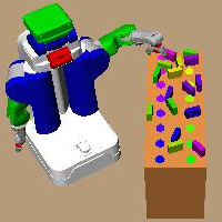
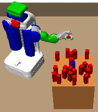
The algorithmic contribution is the construction of two sampling-based planning algorithms that exploit the factored, compositional structure of the solution space to draw samples using conditional samplers. These algorithms search in a combined space that includes the discrete structure (which high-level operations, such as “pick” or “place” happen in which order) and parameters (particular continuous parameters of the actions) of a solution. Theoretically, these algorithms are probabilistically complete when given a set of sampling primitives that cover the appropriate spaces with probability one. Practically, they can solve complex instances of task-and-motion planning problems as well as problems involving non-prehensile manipulation problems.

2 Related Work

inline, color=blue!10, linecolor=blue!90, size=]TODO: Relation to mode sampling

Planning problems in which the goal is not just to move the robot without collision but also to operate on the objects in the world have been addressed from the earliest days of manipulation planning (Lozano-Pérez, 1981; Lozano-Pérez et al., 1987; Wilfong, 1988). Alami et al. (1990, 1994) decomposed manipulation problems using a manipulation graph that represents connected components of the configuration space given by a particular robot grasp. They observed that solutions are alternating sequences of transit and transfer paths corresponding to the robot moving while its hand is empty and the robot moving while holding an object. Vendittelli et al. (2015) proved a manipulation planning with a robot and two movable obstacles is decidable by providing a complete decomposition-based algorithm. Deshpande et al. (2016) extended this result to general, prehensile task and motion planning. Maintaining an explicit characterization of the free configuration space can be prohibitively expensive in high-dimensional planning problems.

Siméon et al. (2004) extended the work of Alami et al. (1990, 1994) by using probabilistic roadmaps (PRMs) (Kavraki et al., 1996) to approximate each component of the configuration space. The aSyMov system (Cambon et al., 2009) generalizes this strategy to task and motion planning with significant discrete structure. It uses a heuristic computed by planning at just the symbolic level to guide the geometric exploration of its roadmaps. Plaku and Hager (2010) also use symbolic planning to influence geometric planning but for biasing sampling instead of guiding the search.

Stilman and Kuffner (2006); Stilman et al. (2007) introduced the problem of robotic navigation among movable obstacles (NAMO), robotic motion planning in a reconfigurable environment. They provide an algorithm for solving monotonic problem instances, problems that require moving each object at most one time. Van Den Berg et al. (2009) developed a probabilistically complete algorithm for robustly feasible NAMO problems. Krontiris and Bekris (2015, 2016) extended the work of Stilman and Kuffner (2006); Stilman et al. (2007) to nonmonotonic rearrangement problems, which require moving a set of objects from to specified goals poses, by using their algorithm as a primitive within a larger, complete search. These algorithms are each specialized to a subclass of manipulation planning.

Hauser and Ng-Thow-Hing (2011) introduced a framework and algorithm multi-modal motion planning, motion planning in overlapping spaces of non-uniform dimensionality. Barry et al. (2013); Barry (2013) considered multi-modal motion planning using bidirectional rapidly-exploring random trees (RRT-Connect). Vega-Brown and Roy (2016) extended these ideas to optimal planning with differential constraints. Because these approaches do not exploit any factoring present within a problem, they must sample entire states at once and are unable to take advantage of powerful heuristics to guide their search,

Dornhege et al. (2009, 2013) introduced semantic attachments, external predicates evaluated on a geometric representation of the state, to integrate geometric reasoning into artificial intelligence planners. Their algorithms assume a finite set of primitive actions which restricts them to discrete control-spaces. They evaluate semantic attachments within their search which results in unnecessarily computing many expensive motion plans.

Kaelbling and Lozano-Pérez (2011) introduced generators to select predecessor states in a goal regression search (HPN). Garrett et al. (2015) gave an algorithm (HBF) for planning in hybrid spaces by using approximations of the planning problem to guide the backward generation of successor actions to be considered in a forward search. Both approaches requires that generators are specified according to an inverse model in order to be compatible with their backward searches. Additionally, both approaches integrate search and sampling preventing them from leveraging discrete search algorithms as blackbox subroutines.

Pandey et al. (2012); de Silva et al. (2013) use hierarchical task networks (HTNs) (Erol et al., 1994) to guide a search over plan skeletons, discrete sequences of actions with unbound continuous variables, using knowledge about the task decomposition. The search over plan skeletons backtracks in the event that it is unable to bind the free continuous variables of a skeleton. Lozano-Pérez and Kaelbling (2014) take a similar approach but leverage constraint satisfaction problem (CSP) solvers operating on discretized variable domains to bind the free variables. Lagriffoul et al. (2012, 2014) also search over plan skeletons but are able to prune some plan skeletons from consideration using computed bounds on the constraints. For each plan skeleton under consideration, they generate a set of approximate linear constraints, e.g. from grasp and placement choices, and use linear programming to compute a valid assignment of continuous values or determine that one does not exist. Similarly, Toussaint (2015); Toussaint and Lopes (2017) formulate the binding of geometric variables as a nonlinear constrained optimization problem and use a hierarchy of bounds on the nonlinear program to prune plan skeletons. Because binding and pruning operate globally on entire plan skeletons, these approaches are unable to identify individual variables and constraints that primarily contributed to infeasibility. Thus, the search over plan skeletons may evaluate many similar plan skeletons that exhibit the same behavior. In contrast, by reasoning locally about individual conditional samplers, our focused algorithm is able to retain samples that satisfy their associated constraints and focus the subsequent search and sampling on conditional samplers that failed to produce satisfactory samples.

The FFRob algorithm of Garrett et al. (2014) samples a set of object poses and robot configurations and then plans with them using a search algorithm that incorporates geometric constraints in its heuristic. An iterative version of FFRob that repeats this process until a solution is found is probabilistically complete and exponentially convergent (Garrett et al., 2017a). Our incremental algorithm can be seen as generalizing this strategy of iteratively sampling then searching from pick-and-place domains to domains with arbitrary conditional samplers.

Erdem et al. (2011) plan at the task-level using a boolean satisfiability (SAT) solver, initially ignoring geometric constraints, and then attempt to produce motion plans satisfying the task-level actions. If an induced motion planning problem is infeasible, the task-level description is updated to indicate motion infeasibility using a domain-specific diagnostic interface.  Dantam et al. (2016) extend this work by using a satisfiability modulo theories (SMT) solver to incrementally add new constraints and restart the task-level search from its previous state. Their approach also adjusts to motion planning failures automatically and in a way that allows previously failed motion planning queries to be reconsidered. The algorithms of Erdem et al. (2011) and Dantam et al. (2016) both assume an a priori discretization of all continuous values apart from configurations, for example, objects placements.  Srivastava et al. (2014) remove this restriction by using symbolic references to continuous parameters. Upon finding a task-level plan, they use a domain-specific interface, like Erdem et al. (2011), to bind values for symbolic references and update the task-level description when none are available. Our focused algorithm is related to these approaches in that it lazily evaluates constraints and plans with lazy samples before real values. However, it is able to automatically manage its search and sampling in a probabilistically complete manner using each individual conditional sampler as a blackbox, without the need of a domain-specific interface.

Our work captures many of the insights in these previous approaches in a general-purpose framework. It also highlights the role of factoring in developing efficient algorithms for sampling relevant values and searching discretized spaces.

3 Factored Transition System

We begin by defining a general class of models for deterministic, observable, discrete-time, hybrid systems. These systems are hybrid in that they have mixed discrete-continuous state and control-spaces. However, they are also discrete-time meaning that transitions are discrete changes to the hybrid state (Torrisi and Bemporad, 2001). This is in contrast to a continuous-time hybrid systems (Alur et al., 1995, 2000; Henzinger, 2000) which allow continuous transitions described as differential equations. It is possible to address many continuous-time problems in this framework, as long as they can be solved with a finite sequence of continuous control inputs.

Definition 1.

A discrete-time transition system ${\cal S}=\langle{\cal X},{\cal U},{\cal T}\rangle$ is defined by a set of states (state-space) ${\cal X}$, set of controls (control-space) ${\cal U}$, and a transition relation ${\cal T}\subseteq{\cal X}\times{\cal U}\times{\cal X}$.

For many physical systems, ${\cal T}$ is a transition function from ${\cal X}\times{\cal U}$ to ${\cal X}$. We are interested in controlling a transition system to move from a given initial state to a state within a goal set.

Definition 2.

A problem ${\cal P}=\langle x^{0},X^{*},{\cal S}\rangle$ is an initial state $x^{0}\subseteq{\cal X}$, a set of goal states $X^{*}\subseteq{\cal X}$, and a transition system ${\cal S}$.

Definition 3.

A plan for a problem ${\cal P}$ is finite sequence of $k$ control inputs $(u^{1},...,u^{k})$ and $k$ states $(x^{1},...,x^{k})$ such that $(x^{i-1},u^{i},x^{i})\in{\cal T}$ for $i\in\{1,...,k\}$ and $x^{k}\in X^{*}$.

When ${\cal T}$ is a transition function, a plan can be uniquely identified by its sequence of control inputs.

3.1 Factoring

We are particularly interested in transition systems that are factorable. As we will show in sections 6 and 8, factored structure is useful for developing efficient methods for sampling and searching transition systems.

Definition 4.

A factored transition system is a transition system with state-space $\bar{\cal X}={\cal X}_{1}\times...\times{\cal X}_{m}$ and control-space $\bar{\cal U}={\cal U}_{1}\times...\times{\cal U}_{n}$ that is defined by $m$ state variables $\bar{x}=(x_{1},...,x_{m})$ and $n$ control variables $\bar{u}=(u_{1},...,u_{n})$.

The transition relation is a subset of the transition parameter-space ${\cal T}\subseteq\bar{\cal X}\times\bar{\cal U}\times\bar{\cal X}$ Valid transitions are $(x_{1},...,x_{m},u_{1},...,u_{n},x^{\prime}_{1},...,x^{\prime}_{m})\in{\cal T}$. To simplify notation, we will generically refer to each $x_{p}$, $u_{p}$, or $x^{\prime}_{p}$ in a transition as a parameter $z_{p}$ where $p\in\{1,...,2m+n\}=\Theta$ indexes the entire sequence of variables. inline, color=blue!10, linecolor=blue!90, size=]TODO: Make $x_{p}$, $u_{p}$, or $x^{\prime}_{p}$?

For a subset of parameter indices $P=(p_{1},...,p_{k})\subseteq\Theta$, let $\bar{z}_{P}=(z_{p_{1}},...,z_{p_{k}})\in\bar{\cal Z}_{P}$ be the combined values and $\bar{\cal Z}_{P}={\cal Z}_{p_{1}}\times...\times{\cal Z}_{p_{k}}$ be the combined domain of the parameters.

Many transition relations are hybrid, in that there is a discrete choice between different types of operation, each of which has a different continuous constraint on the relevant parameters. For example, a pick-and-place problem has transitions corresponding to a robot moving its base, picking each object, and placing each object. In order to expose the discrete structure, we decompose the transition relation ${\cal T}=\bigcup_{a=1}^{\alpha}T_{a}$ into the union of $\alpha$ smaller transition components $T_{a}$. A transition relation $T_{a}$ often is the intersection of several constraints on a subset of the transition parameters.

Definition 5.

A constraint is a pair $C=\langle P,R\rangle$ where $P\subseteq\Theta$ is a subset of parameter indices and $R\subseteq\bar{\cal Z}_{P}$ is a relation on sets ${\cal Z}_{p_{1}},...,{\cal Z}_{p_{k}}$.

A tuple of values that satisfy a constraint is called a constraint element.

Definition 6.

A constraint element $C(v_{p_{1}},...,v_{p_{k}})$ is composed of a constraint $C=\langle P,R\rangle$ and variable values $(v_{p_{1}},...,v_{p_{k}})=\bar{v}_{P}\in R$ for parameter indices $P=(p_{1},...,p_{k})$.

For instance, pick transitions involve constraints that the end-effector initially is empty, the target object is placed stably, the robot’s configuration forms a kinematic solution with the placement, and the end-effector ultimately is holding the object. A constraint decomposition is particularly useful when $|{P}|<<2m+n$; i.e., each individual constraint has low arity. Let $C{\uparrow^{\Theta}}=\{\bar{z}\in\bar{\cal Z}_{\Theta}\mid\bar{z}_{P}\in R\}$ be the extended form of the constraint over all parameter indices $\Theta$. This alternatively can be seen as a Cartesian product of $R$ with $\bar{\cal Z}_{\Theta\setminus P}$ followed by permuting the parameter indices to be in a sorted order. inline, color=blue!10, linecolor=blue!90, size=]TODO: $\bar{P}=(P_{1},...,P_{n})$ as parameter names. $\bar{p}=(p_{1},...p_{n})$ as values?

inline, color=blue!10, linecolor=blue!90, size=]TODO: Say parameter indices instead of parameters in may places?

Definition 7.

A transition component $T_{a}$ is specified as the intersection over a clause of $\beta$ constraints ${\cal C}_{a}=\{C_{1},...,C_{\beta}\}$ where $T_{a}=\bigcap_{b=1}^{\beta}C_{b}^{a}{\uparrow^{\Theta}}$.

Membership in $T_{a}$ is equivalent to the conjunction over membership for each ${\cal C}_{a}$: $[\bar{z}\in T_{a}]\iff\bigwedge_{b=1}^{\beta}[\bar{z}\in C_{b}^{a}{\uparrow^{\Theta}}]$. Within a clause, there are implicit variable domain constraints on each parameter $z_{p}$ of the form $\mathit{Var}_{p}=\langle(z_{p}),{\cal Z}_{p}\rangle$. Finally, the transition relation ${\cal T}$ is the union of $\alpha$ clauses $\{{\cal C}_{1},...,{\cal C}_{\alpha}\}$. Membership in ${\cal T}$ is equivalent to the disjunction over membership for each ${\cal T}$: $[\bar{z}\in{\cal T}]\iff\bigvee_{a=1}^{\alpha}[\bar{z}\in T_{a}]$. Thus, membership in ${\cal T}$ is a logical expression in disjunctive normal form over literals $[\bar{z}\in C_{b}^{a}{\uparrow^{\Theta}}]$.

Factoring the transition relation can expose constraints that have a simple equality form. Equality constraints are important because they transparently reduce the dimensionality of the transition parameter-space.

Definition 8.

A constant equality constraint $\langle(z_{p}),\{\kappa\}\rangle$ (denoted $z_{p}=\kappa$) indicates that parameter $z_{p}$ has value $\kappa$.

Definition 9.

A pairwise equality constraint $\langle(z_{p},z_{p^{\prime}}),\{(v,v)\mid v\in{\cal Z}_{p}\cap{\cal Z}_{p^{\prime}}\}\rangle$ (denoted $z_{p}=z_{p^{\prime}}$) indicates that parameters $z_{p},z_{p^{\prime}}$ have the same value.

For many high-dimensional systems, the transition relation is sparse, meaning its transitions only alter a small number of the state variables at a time. Sparse transition systems have transition relations where each clause contains pairwise equality constraints $x_{p}=x^{\prime}_{p}$ for most state variables $p$. Intuitively, most transitions do not change most state variables.

The initial state $\bar{x}^{0}$ and set of goal states $\bar{X}^{*}$ can be specified using clauses ${\cal C}_{0}$ and ${\cal C}_{*}$ defined solely on state variables. Because $\bar{x}^{0}$ is a single state, its clause is composed of constant equality constraints.

3.2 Constraint Satisfaction

inline, color=blue!10, linecolor=blue!90, size=]TODO: Choose $c$ for clause?

Planning can be thought of as a combined search over discrete clauses and hybrid parameter values. To select a type is to select a clause from the transition relation; to select its parameters is to select the $\bar{x},\bar{u},\bar{x}^{\prime}$ values.

Definition 10.

A finite sequence of transition components $\vec{a}=(a_{1},...,a_{k})$ is a plan skeleton (Lozano-Pérez and Kaelbling, 2014).

For example, solutions to pick-and-place problems are sequences of move, pick, move-while-holding, and place clauses involving the same object.

Definition 11.

The plan parameter-space for a plan skeleton $\vec{a}=(a_{1},...,a_{k})$ is an alternating sequence of states and controls $(\bar{x}^{0},\bar{u}^{1},\bar{x}^{1},...,\bar{u}^{k},\bar{x}^{k})=\vec{z}\in\bar{\cal X}\times(\bar{\cal U}\times\bar{\cal X})^{k}=\vec{\cal Z}$.

Here, we generically refer to each variable in the plan parameter-space as $z_{p}$ where now $p\in\{1,...,m+k(m+n)\}=\Theta$. When applying the constraints for clause $a_{t}$, plan state $\bar{x}^{t-1}$ is the transition state $\bar{x}$ and likewise $\bar{x}^{t}$ is $\bar{x}^{\prime}$. Solutions using this skeleton must satisfy a single clause of all plan-wide constraints ${\cal C}_{\vec{a}}={\cal C}_{0}\cap{\cal C}_{a_{1}}\cap...\cap{\cal C}_{a_{k}}\cap{\cal C}_{*}.$

Definition 12.

A set of constraints ${\cal C}$ is satisfiable if there exists parameter values $\vec{z}\in\vec{Z}$ such that $\bar{z}\in\bigcap_{C\in{\cal C}}C{\uparrow^{\Theta}}$.

Definition 13.

A problem ${\cal P}$ is feasible if there exists a plan skeleton $\vec{a}$ that ${\cal C}_{\vec{a}}$ is satisfiable.

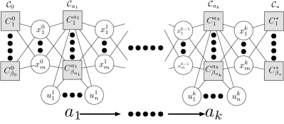
For a given plan skeleton, finding satisfying parameter values $\vec{z}$ is a hybrid constraint satisfaction problem. The joint set of constraints forms a constraint network, a bipartite graph between constraints and parameters (Dechter, 1992; Lagriffoul et al., 2014). An edge between a constraint node $C=\langle P,R\rangle$ and state or control node $x^{t-1}_{p}$, $u^{t}_{p}$, or $x^{t}_{p}$ is defined if and only if $p\in P$. Figure 2 displays a general constraint network. Many transition systems in practice will have constraint networks with many fewer edges because each $P$ contains only a small number of parameters.

Figure 2: A constraint network for a generic plan skeleton $\vec{a}=(a_{1},...,a_{k})$ and parameters $\vec{z}=(\bar{x}^{0},\bar{u}^{1},\bar{x}^{1},...,\bar{u}^{k},\bar{x}^{k})$.

inline, color=blue!10, linecolor=blue!90, size=]TODO: Modeling mode systems

inline, color=blue!10, linecolor=blue!90, size=]TODO: $a$ is used for both the clause name and the pose of object $a$

inline, color=blue!10, linecolor=blue!90, size=]TODO: $p,q$ could be used to emphasize the data type

4 Example Transition Systems

We are interested in a general algorithmic framework that can be applied in many factored transition systems. Consider the following two applications and their representation as factored transition systems. We begin with a motion planning application to illustrate the approach, and then describe a pick-and-place application.

4.1 Motion Planning

inline, color=blue!10, linecolor=blue!90, size=]TODO: Constraints must be contained within clauses, so at most can use two of one state variable

inline, color=blue!10, linecolor=blue!90, size=]TODO: Why even bother putting the variables in them then? Could instead just make two for every action

inline, color=blue!10, linecolor=blue!90, size=]TODO: Maybe a constraint is just a set that we give meaning when we pass in parameters

inline, color=blue!10, linecolor=blue!90, size=]TODO: Distinction between parameter values and names

Many motion planning problems may be defined by a bounded configuration space ${\cal Q}\subset\mathbb{R}^{d}$ and collision-free configuration space $Q_{\it free}\subseteq{\cal Q}$. We will consider planning motions composed of a finite sequence of straight-line trajectories $t$ between waypoints $q,q^{\prime}$. Problems are given by an initial configuration $q_{0}\in{\cal Q}$ and a goal configuration $q_{*}\in{\cal Q}$. Motion planning can be modeled as a transition system with state-space $\bar{\cal X}={\cal Q}$ and control-space $\bar{\cal U}={\cal Q}^{2}$. The transition relation ${\cal T}=\{{\cal C}_{Move}\}$ has a single clause

$${\cal C}_{Move}=\{\mathit{Motion},\mathit{CFree}\}.$$

The transition relation does not exhibit any useful factoring. A motion constraint $\mathit{Motion}$ enforces $u_{t}$ is a straight-line trajectory between $x_{q}$ and $x_{q}^{\prime}$.

$$\mathit{Motion}=\langle(x_{q},u_{t},x_{q}^{\prime}),\{ (q,t,q^{\prime})\mid q,q^{\prime}\in{\cal Q}^{2},$$

$$t(\lambda)=\lambda q+(1-\lambda)q^{\prime}\}\rangle$$

A collision-free constraint $\mathit{CFree}$ ensures all configurations on the trajectory are not in collision.

$$\mathit{CFree}=\langle(u_{t}),\{t\mid\forall\lambda\in[0,1].\;t(\lambda)\in Q_{\it free}\}\rangle.$$

The initial clause is ${\cal C}_{0}=\bar{x}^{0}=\{x_{q}=q_{0}\}$ and the goal clause is ${\cal C}_{*}=\{x_{q}=q_{*}\}$. inline, color=blue!10, linecolor=blue!90, size=]TODO: Zi: is q index or state or control? q ∈Q? Does t denote discretized time steps or state?

inline, color=blue!10, linecolor=blue!90, size=]TODO: Make the robot’s variable be named $R$?

The system state could alternatively be described as $\bar{x}=(x_{j_{1}},...,x_{j_{d}})$ where $j$ is a single robot degree-of-freedom. For simplicity, we combine individual degrees of freedom included within the same constraints into a single variable. This is possible because the set of robot joints always occurs together when mentioned as parameters within motion and kinematic constraints.

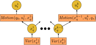
Figure 3 displays a constraint network for a plan skeleton of length $k$. Because the transition relation has a single clause, all solutions have this form. Dark gray circles are parameters, such as the initial and final configurations, that are constrained by constant equality. Free parameters are yellow circles. Constraints are orange rectangles.

Figure 3: Motion planning plan skeleton of length $k$.

4.2 Pick-and-Place Planning

A pick-and-place problem is defined by a single robot with configuration space ${\cal Q}\subset\mathbb{R}^{d}$, a finite set of moveable objects ${\cal O}$, a set of stable placement poses ${\cal S}_{o}\subset\text{SE}(3)$ for each object $o\in{\cal O}$, and a set of grasp poses relative to the end-effector ${\cal G}_{o}\subset\text{SE}(3)$ for each object $o\in{\cal O}$. The robot has a single manipulator that is able to rigidly attach itself to a single object at a time when the end-effector $g$ performs a grasping operation. As before, the robot can execute straight-line trajectories $t$ between waypoints $q,q^{\prime}$.

inline, color=blue!10, linecolor=blue!90, size=]TODO: SE(3) but I consider 2d examples?

Pick-and-place problems can be modeled as a transition system with state-space $\bar{\cal X}={\cal Q}\times\text{SE}(3)^{|{\cal O}|}\times(\{\textbf{None}\}\cup{\cal O})$. States are $\bar{x}=(x_{q},x_{o_{1}},...,x_{o_{|\cal O|}},x_{h})$. Let $h\in{\cal O}$ indicate that the robot is holding object $h$ and $h=\textbf{None}$ indicate that the robot’s gripper is empty. When $h=o$, the pose $x_{o}$ of object $o$ is given in the end-effector frame. Otherwise, $x_{o}$ is relative to the world frame. By representing attachment as a change in frame, the pose of an object remains fixed, relative to the gripper, as the robot moves. Controls are pairs $\bar{u}=(u_{t},u_{g})$ composed of trajectories $u_{t}$ and boolean gripper force commands $u_{g}$. Let $u_{g}=\textbf{True}$ correspond to sustaining a grasp force and $u_{g}=\textbf{False}$ indicate applying no force.

The transition relation ${\cal T}$ has $1+3|{\cal O}|$ clauses because pick, move-while-holding, and place depend on $o$:

$${\cal T}=\{{\cal C}_{Move}\}\cup\{{\cal C}_{MoveH}^{o},{\cal C}_{Pick}^{o},{\cal C}_{\mathit{P}lace}^{o}\mid o\in{\cal O}\}.$$

${\cal C}_{\mathit{Move}}$ and ${\cal C}_{\mathit{MoveH}}^{o}$ clauses correspond to the robot executing a trajectory $u_{t}$ while its gripper is empty or holding object $o$:

$${\cal C}_{\mathit{Move}}= \{\mathit{Motion},\mathit{CFree},x_{h}=\textbf{None},x_{h}=x_{h}^{\prime},$$

$$u_{g}=\textbf{False}\}\;\cup\{x_{o^{\prime}}=x^{\prime}_{o^{\prime}},\mathit{CFree}_{o^{\prime}}\mid o^{\prime}\in{\cal O}\}$$

$${\cal C}_{\mathit{MoveH}}^{o}= \{\mathit{Motion},\mathit{CFreeH}_{o},x_{h}=o,x_{h}=x_{h}^{\prime},$$

$$u_{g}=\textbf{True}\}\;\cup\{\mathit{CFreeH}_{o,o^{\prime}}\mid o^{\prime}\in{\cal O},o\neq o^{\prime}\}.$$

$\mathit{CFree}_{o}$ is a constraint containing robot trajectories $u_{t}$ and object $o$ poses $x_{o}$ that are not in collision with each other. $\mathit{CFreeH}_{o}$ is a constraint composed of robot trajectories $u_{t}$ and object $o$ grasps $x_{o}$ relative to the end-effector that are not in collision with the environment. $\mathit{CFreeH}_{o,o^{\prime}}$ is a constraint containing robot trajectories $u_{t}$, object $o$ grasps $x_{o}$ relative to the end-effector, and object $o^{\prime}$ poses $x_{o}^{\prime}$ that are not in collision with each other.

${\cal C}_{\mathit{Pick}}^{o}$ and ${\cal C}_{\mathit{Place}}^{o}$ clauses correspond to instantaneous changes in what the gripper is holding:

$${\cal C}_{\mathit{Pick}}^{o}= \{\mathit{Stable}_{o},\mathit{Grasp}_{o}^{\prime},\mathit{Kin}_{o},x_{q}=x_{q}^{\prime},x_{h}=\textbf{None},$$

$$x_{h}^{\prime}=o\}\;\cup\{x_{o^{\prime}}=x^{\prime}_{o^{\prime}}\mid o^{\prime}\in{\cal O},o\neq o^{\prime}\}$$

$${\cal C}_{\mathit{Place}}^{o}= \{\mathit{Grasp}_{o},\mathit{Stable}_{o}^{\prime},\mathit{Kin}^{\prime}_{o},x_{q}=x_{q}^{\prime},x_{h}=o,$$

$$x_{h}^{\prime}=\textbf{None}\}\;\cup\{x_{o^{\prime}}=x^{\prime}_{o^{\prime}}\mid o^{\prime}\in{\cal O},o\neq o^{\prime}\}.$$

As a result, they do not involve any control variables. $\mathit{Grasp}_{o}=\langle(x_{o}),{\cal G}_{o}\rangle$ is a constraint that $x_{o}$ is a grasp transform from the object frame to the end-effector frame. Let $\mathit{Grasp}^{\prime}_{o}=\langle(x_{o}^{\prime}),{\cal G}_{o}\rangle$ be the same constraint but on $x_{o}^{\prime}$. Similarly, $\mathit{Stable}_{o}=\langle(x_{o}),{\cal S}_{o}\rangle$ is a constraint that $x_{o}$ is a stable placement, and $\mathit{Stable}^{\prime}_{o}=\langle(x_{o}^{\prime}),{\cal S}_{o}\rangle$. Finally, $\mathit{Kin}_{o}$ is a constraint composed of kinematic solutions involving object $o$ for a grasp $g$, pose $p$, and robot configuration $q$:

$$\mathit{Kin}_{o}=\langle(x_{o}^{\prime},x_{o},x_{q}),\{(g,p,q)\mid\textnormal{kin}(q)=pg^{-1}\}\rangle.$$

$\mathit{Kin}_{o}^{\prime}$ is the equivalent constraint but on state variables $(x_{o},x_{o}^{\prime},x_{q})$, where $x_{o}$ and $x_{o}^{\prime}$ are swapped. Because $\mathit{Kin}_{o}$ and $\mathit{Kin}_{o}^{\prime}$ refer to the same relation and only involve different parameters, we will just refer to $\mathit{Kin}_{o}$. inline, color=blue!10, linecolor=blue!90, size=]TODO: Ensure I keep the correct grasp, pose $\mathit{Kin}$ order

Pick-and-place transition systems are substantially factorable. Each constraint involves at most 3 variables. Additionally, in each clause, many variables are entirely constrained by equality. For ${\cal C}_{\mathit{Move}},{\cal C}_{\mathit{MoveH}}^{o}$ clauses, only half of the variables are not constrained by equality: $\{x_{q},u_{t},x_{q}^{\prime}\}\cup\{x_{o^{\prime}}\mid o^{\prime}\in{\cal O}\}.$ For ${\cal C}_{\mathit{Pick}}^{o},{\cal C}_{\mathit{Place}}^{o}$ clauses, only $\{x_{o},x_{o}^{\prime},x_{q}\}$ variables are not constrained by equality. inline, color=blue!10, linecolor=blue!90, size=]TODO: Should I use upper case letters for objects to indicate that they are names?

Figure 4: The initial state (left) and goal constraints (right) for a pick-and-place problem involving a square robot $R$ and movable circle objects $A$ and $B$.

inline, color=blue!10, linecolor=blue!90, size=]TODO: Change $C_{0}$ in this figure

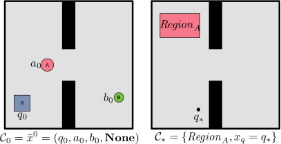
We will use the pick-and-place problem shown in figure 4 with two movable objects $A,B$ as a running example. The initial state $\bar{x}^{0}=(q_{0},a_{0},b_{0},\textbf{None})$ is fully specified using equality constraints ${\cal C}_{0}=\{\bar{x}_{q}=q_{0},\bar{x}_{A}=a_{0},\bar{x}_{B}=b_{0},\bar{x}_{h}=\textbf{None}\}$. We assume that $a_{0}$ and $b_{0}$ are stable poses: $a_{0}\in{\cal S}_{A}$ and $b_{0}\in{\cal S}_{B}$. The goal states $\bar{X}^{*}$ are given as constraints ${\cal C}_{*}=\{\mathit{Region},x_{q}=q_{*}\}$ where the region constraint $\mathit{Region}_{A}=\langle(x_{A}),{\cal R}_{A}\rangle$, for ${\cal R}_{A}\subseteq{\cal S}_{A}$ is a subset of the stable placements for object $A$.

A useful consequence of factoring is that the same control values $\bar{u}$ can be considered in many transitions. Consider the two candidate transitions in figure 5, both using the same control trajectory $u_{t}$. The application of $u_{t}$ in the left figure results in a valid transition for clause $\mathit{Move}$. In fact, for a majority of the combinations of placements of $x_{A}$, $x_{B}$, $u_{t}$ is a valid transition. Thus, for a single value of $u_{t}$, we are implicitly representing many possible transitions. The right figure, however, shows an instance in which this $u_{t}$ does not correspond to a legal transition as it would result in a collision with $B$, thus violating $\mathit{CFree}_{B}$.

Figure 5: A valid transition (left) and an invalid transition (right) for the same control trajectory $u_{t}$. The right transition is invalid because it violates the $\mathit{CFree}_{B}$ collision-free constraint.

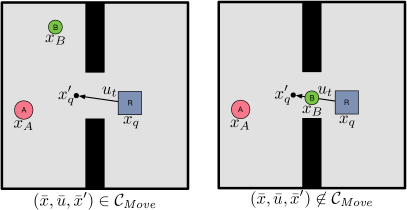
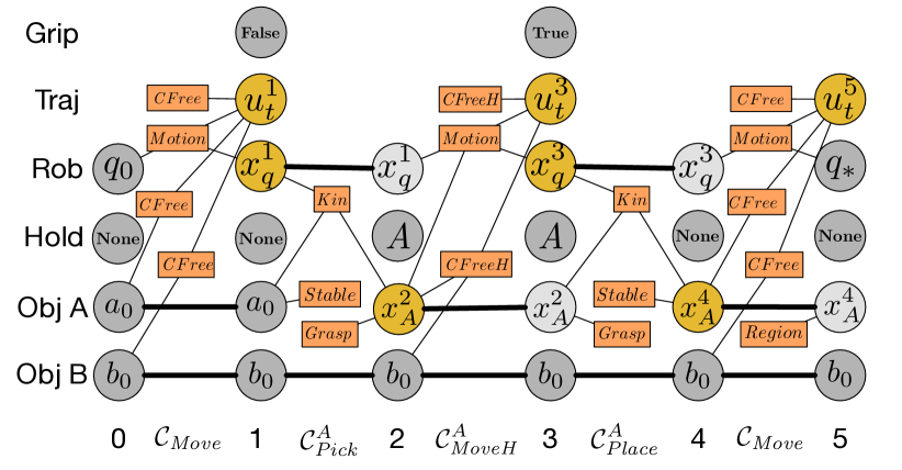
Figure 6 displays the constraint network for a plan skeleton $\vec{a}=(\mathit{Move},\mathit{Pick}^{A},\mathit{MoveH}^{A},\mathit{Place}^{A},\mathit{Move})$ that grabs $A$, places $A$ in $\mathit{Region}_{A}$, and moves the robot to $q_{*}$. Thick edges indicate pairwise equality constraints. Light gray parameters are transitively fixed by pairwise equality. We will omit the constraint subscripts for simplicity. Despite having $29$ total parameters, only $7$ are free parameters. This highlights the strong impact of equality constraints on the dimensionality of the plan parameter-space.

Figure 6: Pick-and-place constraint network for a plan skeleton $\vec{a}=(\mathit{Move},\mathit{Pick}^{A},\mathit{MoveH}^{A},\mathit{Place}^{A},\mathit{Move})$.

5 Sampling-Based Planning

Constraints involving continuous variables are generally characterize uncountably infinite sets, which are often difficult to reason with explicitly. Instead, each constraint can be described using a blackbox, implicit test. A test for constraint $C=\langle{P},{R}\rangle$ is a boolean-valued function $t_{C}:\bar{\cal Z}_{P}\to\{0,1\}$ where $t_{C}(\bar{z}_{P})=[\bar{z}_{P}\in{R}]$. Implicit representations are used in sampling-based motion planning, where they replace explicit representations of complicated robot and environment geometries with collision-checking procedures.

In order to use tests, we need to produce potentially satisfying values for $\bar{z}_{P}=(z_{p_{1}},...,z_{p_{k}})$ by sampling ${\cal Z}_{p_{1}},...,{\cal Z}_{p_{k}}$. Thus, we still require an explicit representation for ${\cal X}_{1},...,{\cal X}_{m}$ and ${\cal U}_{1},...,{\cal U}_{n}$; however, these are typically less difficult to characterize. We will assume ${\cal X}_{1},...,{\cal X}_{m}$, ${\cal U}_{1},...,{\cal U}_{n}$ are each bounded manifolds. This strategy of sampling variable domains and testing constraints is the basis of sampling-based planning (Kavraki et al., 1996). These methods draw values from ${\cal X}_{1},...,{\cal X}_{m}$ and ${\cal U}_{1},...,{\cal U}_{n}$ using deterministic or random samplers for each space and test which combinations of sampled values satisfy required constraints.

Sampling-based techniques are usually not complete over all problem instances. First, they cannot generally identify and terminate on infeasible instances. Second, they are often unable to find solutions to instances that require identifying values from a set that has zero measure in the space from which samples are being drawn. In motion planning, these are problems in which all paths have zero clearance (sometimes called path-goodness), the infimum over distances from the path to obstacles (Kavraki et al., 1998; Kavraki and Latombe, 1998). Thus, sampling-based motion planning algorithms are only theoretically analyzed over the set of problems admitting a path with positive clearance. Conditions similar to positive clearance include an open configuration space (Laumond, 1998), positive $\epsilon$-goodness  (Kavraki et al., 1995; Barraquand et al., 1997; Kavraki and Latombe, 1998) and expansiveness (Hsu et al., 1997; Kavraki and Latombe, 1998).

The ideas of positive clearance (Van Den Berg et al., 2009; Garrett et al., 2017a), positive $\epsilon$-goodness (Berenson and Srinivasa, 2010; Barry, 2013), and expansiveness (Hauser and Latombe, 2010; Hauser and Ng-Thow-Hing, 2011) have been extended to several manipulation planning contexts. In manipulation planning, zero-clearance related properties can take on additional forms. For instance, a goal constraint that two movable objects are placed within a tight region may only admit pairs of goal poses lying on a submanifold of the full set of stable placements (Van Den Berg et al., 2009; Garrett et al., 2017a). At the same time, kinematic constraints resulting from a pick operation define a set lying on a submanifold of the robot’s configuration space (Berenson and Srinivasa, 2010; Garrett et al., 2017a). Thus, these clearance-related properties typically identify a set of anticipated submanifolds, such as a set of inverse kinematic solutions, that can be directly sampled.

More generally, sampling-based algorithms are typically only complete over robustly feasible problems (Karaman and Frazzoli, 2011). When directly applied to factored transitions, a problem is robustly feasible if there exists a plan skeleton $\vec{a}$ such that $\bigcap_{C\in{\cal C}_{\vec{a}}}C{\uparrow^{\Theta}}$ contains an open set in plan-parameter-space $\bar{\cal Z}$.

inline, color=blue!10, linecolor=blue!90, size=]TODO: I could use ${\cal P}_{\vec{a}}$ and $\bar{\cal Z}_{\vec{a}}$

5.1 Dimensionality-reducing constraints

Some problems of interest involve individual constraints that only admit a set of values on a lower-dimensional subset of their parameter-spaces. A dimensionality-reducing constraint $C=\langle P,R\rangle$ is one in which $R\subseteq\bar{\cal Z}_{P}$ does not contain an open set. Consider the ${\mathit{S}table}_{o}$ constraint. The set of satisfying values lies on a 3-dimensional manifold. By our current definition, all plans involving this constraint are not robustly feasible. When a problem involves dimensionality-reducing constraints, we have no choice but to sample at their intersection. This, in general, requires an explicit characterization of their intersection, which we may not have. Moreover, the number of dimensionality-reducing constraint combinations can be unbounded as plan skeletons may be arbitrarily long. However, in some cases, we can produce this intersection automatically using explicit characterizations for only a few spaces.

inline, color=blue!10, linecolor=blue!90, size=]TODO: Do I want to say that we only consider constraints that are low-dimensional for the full domain?

inline, color=blue!10, linecolor=blue!90, size=]TODO: I currently talk about TAMP by only considering poses

Figure 7: Intersection of three constraints, two of them dimensionality-reducing.

We motivate these ideas with an example visualized in figure 7. Consider a plan skeleton $\vec{a}$ with parameters $\Theta=(z_{x},z_{y})$ where ${\cal Z}_{x}={\cal Z}_{y}=(-2,+2)$ and constraints ${\cal C}_{\vec{a}}=\{C_{1},C_{2},C_{3}\}$ where

$$C_{1} =\langle(y),\{-1,0,1\}\rangle$$

$$C_{2} =\langle(x,y),\{(x,y)\mid x+y=0\}\rangle$$

$$C_{3} =\langle(x,y),\{(x,y)\mid x-y\geq 0\}\rangle.$$

The set of solutions $C_{1}{\uparrow^{\Theta}}\cap C_{2}\cap C_{3}=\{(1,-1),(0,0)\}$ is 0-dimensional while the parameter-space is 2-dimensional. This is because $C_{1}$ and $C_{2}$ are both dimensionality-reducing constraints. A uniform sampling strategy where $X,Y\sim\text{Uniform}(-2,+2)$ has zero probability of producing a solution.

To solve this problem using a sampling-based approach, we must sample from $C_{1}{\uparrow^{\Theta}}\cap C_{2}$. Suppose we are unable to analytically compute $C_{1}{\uparrow^{\Theta}}\cap C_{2}$, but we do have explicit representations of $C_{1}$ and $C_{2}$ independently. In particular, suppose we know $C_{2}$ conditioned on values of $y$, $C_{2}(y)=\langle(x),\{-y\}\rangle$. Now, we can characterize $C_{1}{\uparrow^{\Theta}}\cap C_{2}=\{(x,y)\mid y\in R_{1},x\in R_{2}(y)\}=\{(1,-1),(0,0),(-1,1)\}$. With respect to a counting measure on this discrete space, $C_{1}{\uparrow^{\Theta}}\cap C_{2}\cap C_{3}$ has positive measure. This not only gives a representation for the intersection but also suggests the following way to sample the intersection: $Y\sim\text{Uniform}(\{-1,0,+1\})$, $X=-Y$, and reject $(X,Y)$ that does not satisfy $C_{3}$. This strategy is not effective for all combinations of dimensionality-reducing constraints. Suppose that instead $C_{1}=\langle(x,y),\{(x,y)\mid x-y=1\}\rangle$. Because both constraints involve $x$ and $y$, we are unable to condition on the value of one parameter to sample the other. inline, color=blue!10, linecolor=blue!90, size=]TODO: It would be nice if we sampled $X$ as well…

5.2 Intersection of Manifolds

inline, color=blue!10, linecolor=blue!90, size=]TODO: The denseness argument doesn’t depend on the measure stuff. I don’t have to worry about saying a densely sample the coordinate space. Instead, I can just say that I hit the subset of configurations that satisfy this property

In this section, we develop the topological tools to generalize the previous example. Our objective is to show that by making assumptions on each dimensionality reducing constraint individually, we can understand the space formed by the intersection of many dimensionality constraints. First, we overview several topological ideas that we will use (Tu, 2010).

5.2.1 Topological Tools:

A $d$-dimensional manifold $M$ is a topological space that is locally homeomorphic to $d$-dimensional Euclidean coordinate space. Let $d=\dim{M}$ be the dimension of the coordinate space of $M$. An atlas for an $d$-dimensional manifold $M\subseteq\mathbb{R}^{m}$ is a set of charts $\{(U_{\alpha},\varphi_{\alpha}),...\}$ such that $\bigcup_{\alpha}U_{\alpha}=M$. Each chart $(U_{\alpha},\varphi_{\alpha})$ is given by an open set $U_{\alpha}\subseteq M$ and a homeomorphism, a continuous bijection with a continuous inverse, $\varphi:U_{\alpha}\to\mathbb{R}^{d}$. Let $N$ be a regular submanifold of ambient manifold $M$. Then, $\operatorname{codim}{N}=\dim{M}-\dim{N}$ is the codimension of $N$.

Define $T_{x}(M)$ to be the tangent space of manifold $M$ at $x\in M$, which intuitively contains the set of directions in which one can pass through $M$ at $x$. A smooth map of manifolds $f:M\to N$ is submersion at $x\in M$ if its differential, a linear map between tangent spaces, $df_{x}:T_{x}(M)\to T_{f(x)}(N)$ is surjective. When $\dim{M}\geq\dim{N}$, this is equivalent to the Jacobian matrix of $f$ at $x$ having maximal rank equal to $\dim{N}$. When $f$ is a submersion, by the preimage theorem (also called the implicit function theorem and the regular level set theorem), the preimage $f^{-1}(y)$ for any $y\subseteq N$ is a submanifold of $M$ of dimension ${\dim{M}-\dim{N}}$. Similarly, by the local normal submersion theorem, there exists coordinate charts $\varphi$ and $\varphi^{\prime}$ local to $x\in M$ and $f(x)\in N$ such that $f$ is a projection in coordinate space. Thus, the first $\dim{N}$ coordinates of $\varphi(x)$ and $\varphi(f(x))$ are the same and $\varphi(x)$ contains an extra $\operatorname{codim}{N}$ coordinates.

For manifolds $N_{1}$ and $N_{2}$, consider projections $\operatorname{proj}_{1}:(N_{1}\times N_{2})\to N_{1}$ and $\operatorname{proj}_{2}:(N_{1}\times N_{2})\to N_{2}$. For all $\bar{y}=(y_{1},y_{2})\in N_{1}\times N_{2}$, the map

$$(d\operatorname{proj}_{1},d\operatorname{proj}_{2}):T_{\bar{y}}(N_{1}\times N_{2})\to T_{y_{1}}(N_{1})\times T_{y_{2}}(N_{2})$$

is an isomorphism. Thus, the tangent space of a product manifold is isomorphic to the Cartesian product of the tangent spaces of its components.

Let $N_{1},N_{2}$ both be submanifolds of the same ambient manifold $M$. An intersection is transverse if $\forall x\in(N_{1}\cap N_{2}).\;T_{x}(N_{1})+T_{x}(N_{2})=T_{x}(M)$ where

$$T_{x}(N_{1})+T_{x}(N_{2})=\{v+w\mid v\in T_{x}(N_{1}),w\in T_{x}(N_{2})\}.$$

If the intersection $N_{1}\cap N_{2}$ is transverse, then $N_{1}\cap N_{2}$ is a submanifold of codimension

$$\operatorname{codim}(N_{1}\cap N_{2})=\operatorname{codim}{N_{1}}+\operatorname{codim}{N_{2}}.$$

Intuitively, the intersection is transverse if their combined tangent spaces produce the tangent space of the ambient manifold.

5.2.2 Conditional Constraints:

We start by defining conditional constraints, a binary partition of $P$ for a constraint $\langle P,R\rangle$.

inline, color=blue!10, linecolor=blue!90, size=]TODO: Finite chart business only affects algorithms

inline, color=blue!10, linecolor=blue!90, size=]TODO: Projection is open set within

inline, color=blue!10, linecolor=blue!90, size=]TODO: In future work, I can incorporate domain constraints in the projection to allow it to be a manifold. That way, the preimage can guarantee the intersection works

Definition 14.

A conditional constraint $\langle I,O,R\rangle$ for a constraint $C=\langle P,R\rangle$ is a partition of $P$ into a set of input parameters $I$ and a set of output parameters $O$.

Define $\operatorname{proj}_{I}(\bar{z})=\bar{z}_{P}$ to be the set-theoretic projection of $\bar{z}$ onto parameters $P$. Let its inverse, the projection preimage $\operatorname{proj}^{-1}_{I}(\bar{z}_{I})$, be the following:

$$\operatorname{proj}^{-1}_{I}(\bar{z}_{I})=\{\bar{z}_{P}\in R\mid\bar{z}_{P}=(\bar{z}_{I},\bar{z}_{O})\}.$$

Conditional constraints will allow us to implicitly reason about intersections of $\operatorname{proj}_{I}(R)$ rather than $R$ directly. In order to cleanly describe a lower-dimensional space produced by the intersection of several constraints, we will consider a simplified manifold $M$ that is a subset of $R$. Additionally, we will make an assumption regarding the relationship between $\operatorname{proj}_{I}(M)$ and $M$ to use the preimage theorem.

Definition 15.

A conditional constraint manifold $\langle I,O,M\rangle$ for a conditional constraint $\langle I,O,R\rangle$ is a nonempty smooth manifold $M\subseteq R$ such that $\operatorname{proj}_{I}:M\to{\cal Z}_{I}$ is a submersion $\forall\bar{z}_{P}\in M$.

inline, color=blue!10, linecolor=blue!90, size=]TODO: Can just use a version of the original charts for $M$ (i.e. without projection) that is organized to satisfy the submersion theorem. In this case, only need to assume there are a finite set of these charts. This avoids having to worry about parameterized charts. Although, really this kind is a parameterized chart.

In our context, $M$ is a submanifold of $\bar{\cal Z}_{P}={\cal Z}_{P_{1}}\times...\times{\cal Z}_{P_{|P|}}$ because $R\subset\bar{\cal Z}_{P}$. The projection $\operatorname{proj}_{I}=f$ is trivially smooth map between manifold $M$ and product manifold $\bar{\cal Z}_{I}$. Thus, $\operatorname{proj}_{I}$ is a submersion at $\bar{z}_{P}\in M$ when $d{\operatorname{proj}_{I}}:T_{\bar{z}_{P}}(M)\to T_{\bar{z}_{I}}({\cal Z}_{I})$ is surjective. When ${\cal Z}_{I}=\mathbb{R}^{d}$, this is equivalent to the subspace of tangent space $T_{\bar{z}_{P}}(M)$ on parameters $I$ having rank $d$. A more intuitive interpretation is locally at $\bar{z}_{P}$, there exists coordinates to control $M$ in any direction of $I$. This restriction is used to ensure that the intersection of $M$ and other conditional constraint manifolds will not be transdimensional. This implies the preimage $\operatorname{proj}_{I}^{-1}(\bar{z}_{I})$ for particular values of input parameters $\bar{z}_{I}\in\operatorname{proj}_{I}(M)$ is a submanifold of $M$ of codimension $\dim\bar{\cal Z}_{I}$. Importantly, $\operatorname{proj}_{I}(M)$ is an open set within $\bar{\cal Z}_{I}$. This is the key consequence of the submersion assumption which is useful when intersecting arbitrary conditional constraint manifolds. inline, color=blue!10, linecolor=blue!90, size=]TODO: This is similar to only considering an open subset of the configuration space when doing motion planning

inline, color=blue!10, linecolor=blue!90, size=]TODO: The incremental construction perspective is nice because it is more clear where the new degrees of freedom come from

inline, color=blue!10, linecolor=blue!90, size=]TODO: Each $\bar{z}_{O_{i}}$ is effectively one variable (vector)

inline, color=blue!10, linecolor=blue!90, size=]TODO: Vector projection

inline, color=blue!10, linecolor=blue!90, size=]TODO: Just globally reorder the indices

Suppose we are given a set of conditional constraint manifolds $\{\langle I_{1},O_{1},M_{1}\rangle,...,\langle I_{n},O_{n},M_{n}\rangle\}$. Let $\Theta=\bigcup_{j=1}^{n}P_{j}$ be the set of parameters they collectively mention. Let $S=\bigcap_{j=1}^{n}M_{j}{\uparrow^{\Theta}}$ be their intersection when each constraint is extended on $\Theta$. We now present the main theorem which gives a sufficient condition for when $S$ is a submanifold of $\bar{\cal Z}_{\Theta}$. This theorem is useful because it identifies when the intersection of several possibly dimensionality-reducing constraints is a space that we can easily characterize.

inline, color=blue!10, linecolor=blue!90, size=]TODO: No need to provide charts. Can also change charts inductively

inline, color=blue!10, linecolor=blue!90, size=]TODO: Maybe I should do the subtractive form of this that asserts all manifolds are extended?

inline, color=blue!10, linecolor=blue!90, size=]TODO: I could intersect with its level sets or something if I preferred

inline, color=blue!10, linecolor=blue!90, size=]TODO: The level sets are disjoint

inline, color=blue!10, linecolor=blue!90, size=]TODO: I can just say that locally homeomorphic

inline, color=blue!10, linecolor=blue!90, size=]TODO: Can I do this directly by examining each element?

Theorem 1.

If $\{O_{1},...,O_{n}\}$ is a partition of $\Theta$ and there exists an ordering of $(\langle I_{1},O_{1},M_{1}\rangle,...,\langle I_{n},O_{n},M_{n}\rangle)$ such that $\forall i=\{1,...,n\}\;I_{i}\subseteq\bigcup_{j=1}^{i-1}O_{j}$, then $S=\bigcap_{j=1}^{n}M_{j}{\uparrow^{\Theta}}$ is a submanifold of $\bar{\cal Z}_{\Theta}$ of codimension $\sum_{j=1}^{n}\operatorname{codim}{M_{j}}$.

Proof.

Define $\Theta_{i}=\bigcup_{j=1}^{i}P_{j}$ to be union of the first $i$ sets of parameters. Notice that $\Theta_{i}=\bigcup_{j=1}^{i}O_{j}$ follows from the second assumption. Let $S_{i}=\bigcap_{j=1}^{i}M_{j}{\uparrow^{\Theta_{i}}}$ be the intersection of the first $i$ constraint manifolds over parameters $\Theta_{i}$. On the final intersection, $\Theta_{n}=\Theta$ and $S_{n}=S$. We can also write $S_{i}$ recursively as ${S_{i}=S_{i-1}{\uparrow^{\Theta_{i}}}\cap M_{i}{\uparrow^{\Theta_{i}}}}$ where $S_{0}=\emptyset$. Here, $S_{i-1}$ and $M_{i}$ are extended by Cartesian products with $\bar{\cal Z}_{O_{i}}$ and $\bar{\cal Z}_{\Theta_{i}\setminus P_{i}}$ respectively.

We proceed by induction on $i$. For the base case, $I_{1}=\bigcup_{j=1}^{0}O_{j}=\emptyset$. Thus, $S_{0}{\uparrow^{\Theta_{1}}}=\bar{\cal Z}_{O_{1}}$ and $M_{1}{\uparrow^{\Theta_{1}}}=M_{1}$. Since, $M_{1}\subseteq\bar{\cal Z}_{O_{1}}$,

$$S_{1}=(S_{0}{\uparrow^{\Theta_{1}}}\cap M_{1}{\uparrow^{\Theta_{1}}})=(\bar{\cal Z}_{O_{1}}\cap M_{1})=M_{1}$$

is a submanifold of codimension $\operatorname{codim}{M_{1}}$ within $\bar{\cal Z}_{O_{1}}$.

For the inductive step, we assume that after the ${(i-1)}$th intersection, $S_{i-1}$ is a submanifold of codimensionality $\operatorname{codim}{S_{i-1}}$ on parameters $\Theta_{i-1}$. We will show that $S_{i}$ is a manifold of codimension $\operatorname{codim}{S_{i-1}}+\dim{M_{i}}$ on parameters $\Theta_{i}$. By isomorphism of product manifold tangent spaces, $\forall\bar{z}\in S_{i-1}{\uparrow^{\Theta_{i}}}$, $T_{\bar{z}}(S_{i-1}{\uparrow^{\Theta_{i}}})$ is isomorphic to $T_{\bar{z}_{\Theta_{i-1}}}(S_{i-1})\times T_{\bar{z}_{O_{i}}}(\bar{\cal Z}_{O_{i}})$. Similarly, $\forall\bar{z}\in M_{i}{\uparrow^{\Theta_{i}}}$, $T_{\bar{z}}(M_{i}{\uparrow^{\Theta_{i}}})$ is isomorphic to $T_{\bar{z}_{P_{i}}}(M_{i})\times T_{\bar{z}_{\Theta_{i}\setminus P_{i}}}(\bar{\cal Z}_{\Theta_{i}\setminus P_{i}})$. As a result, the projection for the extended constraint $d{\operatorname{proj}_{\Theta_{i-1}}}:T_{\bar{z}}(M_{i}{\uparrow^{\Theta_{i}}})\to T_{\bar{z}_{\Theta_{i-1}}}(\bar{\cal Z}_{\Theta_{i-1}})$ is itself surjective for all $\bar{z}$ and therefore is a submersion.

Because $S_{i}\subseteq\bar{\cal Z}_{\Theta_{i}}$, for any $\bar{z}\in S_{i}$, $T_{\bar{z}}(M_{i}{\uparrow^{\Theta_{i}}})+T_{\bar{z}}(S_{i-1}{\uparrow^{\Theta_{i}}})\subseteq T_{\bar{z}}(\bar{\cal Z}_{\Theta_{i}})$ For each $\bar{z}\in S_{i}$, consider any tangent $v\in T_{\bar{z}}(\bar{\cal Z}_{\Theta_{i}})$. Let $v=x+y$ be an orthogonal decomposition of $v$ into a component $x$ defined on parameters $\Theta_{i-1}$ and component $y$ defined on $O_{i}$. The first component $x$ is isomorphic to an element of $T_{\bar{z}}(M_{i}{\uparrow^{\Theta_{i}}})$ because its tangent space is surjective to $\bar{\cal Z}_{\Theta_{i-1}}$. The second component $y$ is isomorphic to an element of $T_{\bar{z}}(S_{i-1}{\uparrow^{\Theta_{i}}})$ by the isomorphism to the product space involving $\bar{\cal Z}_{O_{i}}$. Thus, $T_{\bar{z}}(\bar{\cal Z}_{\Theta_{i}})\subseteq T_{\bar{z}}(M_{i}{\uparrow^{\Theta_{i}}})+T_{\bar{z}}(S_{i-1}{\uparrow^{\Theta_{i}}})$. As a result, $M_{i}{\uparrow^{\Theta_{i}}}$ and $S_{i-1}{\uparrow^{\Theta_{i}}}$ intersect transversally implying that $S_{i}$ is a smooth submanifold of $\bar{\cal Z}_{\Theta_{i}}$ with codimension

$$\operatorname{codim}{M_{i}{\uparrow^{\Theta_{i}}}}+\operatorname{codim}{S_{i-1}{\uparrow^{\Theta_{i}}}}=\operatorname{codim}{M_{i}}+\operatorname{codim}{S_{i-1}}.$$

inline, color=blue!10, linecolor=blue!90, size=]TODO: Generalize this to when the projection is not the full space but a previous submanifold. This allows us to deal with domain constraints.

After $n$ iterations, the entire intersection is a submanifold of codimension $\operatorname{codim}{S}=\operatorname{codim}{M_{1}}+...+\operatorname{codim}{M_{n}}$ in $\Theta$. Let $d_{i}=\dim{M_{i}}-\dim{\bar{\cal Z}_{I_{i}}}$ be the dimension of the submanifold defined by the projection preimage $\operatorname{proj}_{I_{i}}^{-1}(\bar{z}_{I})$. Finally, $\dim S$ can be seen alternatively as the sum of $\sum_{i=1}^{n}d_{i}$, the number of coordinates introduced on each iteration.

$$\dim{S} =\dim\bar{\cal Z}_{\Theta}-\sum_{i=1}^{n}\operatorname{codim}{M_{i}}$$

$$=\dim\bar{\cal Z}_{\Theta}-\sum_{i=1}^{n}\big{(}\dim{\bar{\cal Z}_{P_{i}}}-\dim{M_{i}}\big{)}$$

$$=\dim\bar{\cal Z}_{\Theta}-\sum_{i=1}^{n}\big{(}\dim{\bar{\cal Z}_{O_{i}}}+\dim{\bar{\cal Z}_{I_{i}}}-\dim{M_{i}}\big{)}$$

$$=\sum_{i=1}^{n}\big{(}\dim{M_{i}}-\dim{\bar{\cal Z}_{I_{i}}}\big{)}=\sum_{i=1}^{n}d_{i}$$

∎∎

inline, color=blue!10, linecolor=blue!90, size=]TODO: Show that the manifold story admits samplers

We will call $S$ a sample space when theorem 1 holds. From the partition condition, each parameter must be the output of exactly one conditional constraint manifold. Intuitively, a parameter can only be “chosen” once. From subset condition, each input parameter must be an output parameter for some conditional constraint manifold earlier in the sequence. Intuitively, a parameter must be “chosen” before it can be used to produce values for other parameters. Theorem 1 can be understood graphically using sampling networks. A sampling network is a subgraph of a constraint network using constraints corresponding to conditional constraint manifolds. The graphical relationship between a constraint network and a sampling network is analogous to the relationship between a factor graph and a Bayesian network from probabilistic inference (Jensen, 1996). However, this resemblance is purely structural because constraint networks and sampling networks represent sets given as the intersection of several constraints while graphical models represent joint distributions over sets. Each parameter node in a sampling network has exactly one incoming edge. Directed edges go from input parameters to constraints or constraints to output parameters. Each parameter is the output of exactly one constraint. Finally, the graph is acyclic.

When analyzing robustness properties, we will assume that we are given a set of conditional constraint manifolds ${\cal M}$. This set ${\cal M}$ is typically composed of dimensionality-reducing constraints that have a known analytic form. We may have multiple conditional constraint manifolds per constraint $C$, resulting from the different ways of conditionalizing $C$. Implicit variable domain constraints $\langle(),(x_{i}),{\cal X}_{i}\rangle,\langle(),(u_{j}),{\cal U}_{i}\rangle\in{\cal M}$ for each variable are always present within ${\cal M}$. Given a set of constraints ${\cal C}$ defined on parameters $\Theta$, we can produce the corresponding set of conditional constraint manifolds on $\Theta$ by substituting constraints for the conditional constraint manifolds. For a constraint $C=\langle P,R\rangle$, let ${\cal M}_{C}$ be the set of conditional constraint manifolds $\{\langle I,O,M\rangle,...\}\subseteq{\cal M}$ associated with $C$ by substituting the input and output parameters $I,O$ for each conditional constraint manifold for with the parameters for $P$. For a set of constraints, let ${\cal M}_{\cal C}=\cup_{C\in{\cal C}}{\cal M}_{C}$ be the union for each constraint $C\in{\cal C}$.

Now we generalize our definition of robust feasibility to be with respect to a set of conditional constraint manifolds ${\cal M}$. Note that when ${\cal M}$ is solely composed of variable domain constraints, the new definition is equivalent to the previous definition. Specifying ${\cal M}$ allows us to analyze the set of solutions in a lower-dimensional space $S$ given by the constraint manifolds. Intuitively, a set of constraints is robustly satisfiable ${\cal C}$ if for some parameter values $\bar{z}\in S$, all parameter values $\bar{z}^{\prime}$ in a neighborhood of $\bar{z}$ satisfy ${\cal C}$.

inline, color=blue!10, linecolor=blue!90, size=]TODO: I could also just do just feasible

Definition 16.

A set of constraints ${\cal C}$ is robustly satisfiable with respect to conditional constraint manifolds ${\cal M}$ if there exists a sample space $S=\bigcap_{i=1}^{n}\widehat{M}_{i}$ formed from conditional constraint manifolds $\{\langle I_{1},O_{1},M_{1}\rangle,...,\langle I_{n},O_{n},M_{n}\rangle\}\subseteq{\cal C}_{\cal M}$ where there exists a satisfying $\vec{z}$ with a neighborhood of parameter values ${\cal N}(\vec{z})$ in $S$ such that ${\cal N}(\bar{z})\subseteq\bigcap_{C\in{\cal C}}C{\uparrow^{\Theta}}$.

We are typically interested in evaluating robustness properties with respect to ${\cal M}$ for a set of problems defined with the same transition system ${\cal S}$ instead of for just a single problem ${\cal P}$. Thus, we a define a domain to be a set of problems ${\cal D}$ to be analyzed with respect to a common set of conditional constraint manifolds ${\cal M}$. A domain here is similar to the notion of a domain in automated planning (McDermott et al., 1998) because both fix the dynamics of the system and the objective criteria across a set of problems.

Definition 17.

A domain $\langle{\cal D},{\cal M}\rangle$ is given by a set of problems ${\cal D}$, where each ${\cal P}\in{\cal D}$ has an identical transition system ${\cal S}$, and a set of conditional constraint manifolds ${\cal M}$.

This allows us to describe the robustly feasible subset of problems within a domain.

Definition 18.

A factored transition problem ${\cal P}\in{\cal D}$ within a domain $\langle{\cal D},{\cal M}\rangle$ is robustly feasible if there exists a plan skeleton $\vec{a}$ such that ${\cal C}_{\vec{a}}$ is robustly satisfiable with respect to ${\cal M}$.

inline, color=blue!10, linecolor=blue!90, size=]TODO: I could spell out ${\cal M}$

inline, color=blue!10, linecolor=blue!90, size=]TODO: I think I should include the robustness sampling networks here

5.3 Robust Motion Planning

Our motion planning system involves a single dimensionality reducing constraint $\mathit{Motion}$. The implicit variable domain constraint $\mathit{Var}_{q}=\langle(x_{q}),{\cal Q}\rangle$ has full dimensionality by default. Each straight-line trajectory $t$ is uniquely described by its start configuration $q=t(0)$ and end configuration $q^{\prime}=t(1)$. Thus, we can notate a straight-line trajectory as $t=(q,q^{\prime})\in{\cal Q}^{2}\subseteq\mathbb{R}^{2d}$. As a result, $\mathit{Motion}$ is a $2d$-dimensional submanifold of ${\cal Q}^{4}\subseteq\mathbb{R}^{4d}$. We will consider sample spaces resulting from constraint manifolds ${\cal M}=\{\mathit{Var}_{q},\mathit{Motion}\}$.

Figure 8 shows a sampling network for the generic motion planning constraint network in figure 3. This sampling network uses conditional constraint manifolds $\{\langle(),(x_{q}),\mathit{Var}_{q}\rangle,\langle(x_{q},x_{q}^{\prime}),(u_{t}),\mathit{Motion}\rangle\}$. The projection $\operatorname{proj}_{x_{q},x_{q}^{\prime}}(\mathit{Motion})={\cal Q}^{2}$ and is thus trivially a submersion. The projection preimage $\operatorname{proj}_{x_{q},x_{q}^{\prime}}^{-1}(q,q^{\prime})=\{t\}$ is a single point corresponding to the straight-line trajectory. Thus, the sample space $S\subseteq{\cal Q}^{3k-1}\subseteq\mathbb{R}^{d(3k-1)}$ is a submanifold of dimensionality $d(k-1)$. Intuitively, the space of satisfying values is parametrizable by each configuration $x_{q}^{i}$ for $i=1,...,(k-1)$. As a result, a possible coordinate space of $S$ is ${\cal Q}^{k-1}$ corresponding to Cartesian product of ${\cal Q}$, the variable domain for each $x_{q}^{i}$.

Figure 8: Motion planning sampling network for constraint network in figure 3.

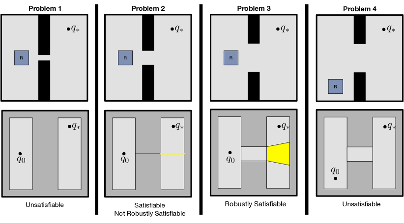
Subject to this sample space, we can analyze robustly feasible motion planning problems. Figure 9 fixes the plan skeleton $\vec{a}=(\mathit{Move},\mathit{Move})$ and investigates robustness properties of four problems varying the environment geometry. The plan skeleton has the following free parameters: $\{u_{t}^{1},x_{q}^{1},u_{t}^{2}\}$. However, $u_{t}^{1},u_{t}^{2}$ can be uniquely determined given $x_{q}^{1}$. The choices of these parameters must satisfy the following constraints:

$$\{ \mathit{Motion}(q_{0},u_{t}^{1},x_{q}^{1}),\mathit{CFree}(u_{t}^{1}),$$

$$\mathit{Motion}(x_{q}^{1},u_{t}^{2},q_{*}),\mathit{CFree}(u_{t}^{2})\}.$$

Varying the environment only affects the $\mathit{CFree}$ constraint. The top row displays a top-down image of the scene and the bottom image shows the robot’s collision-free configuration space $Q_{\mathit{free}}$ in light grey. Linear trajectories contained within the light grey regions satisfy their $\mathit{CFree}$ constraint. The yellow region indicates values of $x_{q}^{1}$ that will result in a plan. Problem 1 is unsatisfiable because no values of $x_{q}^{1}$ result in a plan. Problem 2 has only a 1 dimensional interval of plan, thus it is satisfiable but not robustly satisfiable. Problem 3 has a 2 dimensional region of solutions, so it is robustly satisfiable. Problem 4 is unsatisfiable for the current plan skeleton. However, it is robustly satisfiable for a plan skeleton $\vec{a}=(\mathit{Move},\mathit{Move},\mathit{Move})$.

Figure 9: From left to right, an unsatisfiable, satisfiable (but not robustly satisfiable), robustly satisfiable, and unsatisfiable motion planning problem for a plan skeleton involving two transitions. The top row displays each problem, varying the environment. The bottom row displays the collision-free configuration space $Q_{\mathit{free}}$. Yellow regions of configuration space correspond to values of $x_{q}^{1}$ satisfying the plan skeleton.

inline, color=blue!10, linecolor=blue!90, size=]TODO: Assume objects are open sets?

5.4 Robust Pick-and-Place

inline, color=blue!10, linecolor=blue!90, size=]TODO: I already define dimensionality reducing constraint

In pick-and-place problems, $\mathit{Stable}$, $\mathit{Region}$, $\mathit{Grasp}$, $\mathit{Kin}$, and $\mathit{Motion}$ are all individually dimensionality-reducing constraints. Fortunately, we generally understand explicit representations of these sets. We will consider the following constraint manifolds:

$${\cal M}=\{\mathit{Var}_{q},\mathit{Motion}\}\cup\{\mathit{Stable}_{o},\mathit{Grasp}_{o},\mathit{Kin}_{o}\mid o\in{\cal O}\}.$$

We will only consider problems in which $\dim\mathit{Stable}_{o}=\dim\mathit{Region}_{o}$ in which case $\mathit{Stable}_{o}$ captures the reduction of dimensionality from $\mathit{Region}_{o}$. Again, $\mathit{CFree}$, $\mathit{CFree}_{o}$, $\mathit{CFreeH}_{o}$, and $\mathit{CFreeH}_{o,o^{\prime}}$ are not assumed to be dimensionality-reducing constraints.

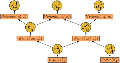
Figure 10 shows a sampling network for the pick-and-place constraint network in figure 6. It uses the following conditional constraint manifolds:

$$\{ \langle(x_{q},x_{q}^{\prime}),(u_{t}),\mathit{Motion}\rangle\}\cup\{\langle(),(x_{o}),\mathit{Stable}_{o}\rangle,$$

$$\langle(),(x_{o}),\mathit{Grasp}_{o}\rangle,\langle(x_{o},x_{o}^{\prime}),(x_{q}),\mathit{Kin}_{o}\rangle\mid o\in{\cal O}\}.$$

The sampling network satisfies the graph theoretic conditions in theorem 1. Additionally, each conditional constraint manifold has full dimensionality in its input parameter-space. $\mathit{Var}_{q}$, $\mathit{Stable}_{o}$ and $\mathit{Grasp}_{o}$ have no input parameters and therefore trivially have full input dimensionality. The projection $\operatorname{proj}_{x_{o},x_{o}^{\prime}}(\mathit{Kin}_{o})$ has full dimensionality under the assumption that the robot gripper’s workspace has positive measure in SE(3). We will consider a manifold subset of $\mathit{Kin}_{o}$ that satisfies the submersion conditions by omitting kinematic singularities. As before, $\operatorname{proj}_{x_{q},x_{q}^{\prime}}(\mathit{Motion})$ has full input dimensionality.

Figure 10: Pick-and-place sampling network for the constraint network in figure 6.

inline, color=blue!10, linecolor=blue!90, size=]TODO: I really do need a move here…

This sampling network structure generalizes to all pick-and-place problems with goal constraints on object poses and robot configurations. Solutions are alternating sequences of $\mathit{Move}$, $\mathit{Pick}$, $\mathit{MoveH}$, and $\mathit{Place}$ transitions where $\mathit{Move}$ and $\mathit{MoveH}$ may be repeated zero to arbitrarily many times. Each new cycle introduces a new grasp parameter, pose parameter, two configuration parameters, and two trajectory parameters. However, the only interaction with the next cycle is through the beginning and ending configurations which serve as the input parameters for the next move transition. Thus, this small set of conditional constraint manifolds is enough to define sample spaces for a large set of pick-and-place problems involving many objects.

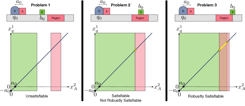
To better visualize a pick-and-place sample space, we investigate a 1-dimensional example where ${\cal Q},{\cal S}_{A},{\cal S}_{B}\subset\mathbb{R}$. Figure 11 fixes the plan skeleton $\vec{a}=(\mathit{MoveH}^{A},\mathit{Place}^{A})$ and investigates robustness properties of three problems varying the initial pose $b_{0}$ of block $B$. The robot starts off holding block $A$ with grasp $a_{0}$, so in the initial state, $x_{h}^{0}=A$ and $x_{A}^{0}=a_{0}$. The robot may only grasp block $A$ when $A$ touches its left or right side. Therefore, the set of grasps ${\cal G}_{A}=\{-a_{0},a_{0}\}$ is finite. Additionally, the kinematic constraint on $(x_{o},x_{o}^{\prime},x_{q})$ results in a plane within $\mathbb{R}^{3}$.

$$\mathit{Kin}_{o}=\langle(x_{o}^{\prime},x_{o},x_{q}),\{q+g=p\mid(g,p,q)\in\mathbb{R}^{3}\}\rangle$$

The goal constraint ${\cal C}_{*}=\{\mathit{Region}_{A}\}$ requires that $A$ be placed within a goal region. The plan skeleton has the following free parameters: $x_{q}^{1}$ is the final robot configuration, $u_{t}^{1}$ is the $\mathit{MoveH}^{A}$ trajectory, and $x_{A}^{2}$ is the final pose of block $A$. Once again, $u_{t}^{1}$ can be uniquely determined given $x_{q}^{1}$. The choices of these parameters must satisfy the following constraints:

$$\{\mathit{Motion}(q_{0},u_{t}^{1},x_{q}^{1}),\mathit{CFreeH}(u_{t}^{1},a_{0}),\mathit{CFreeH}(u_{t}^{1},a_{0},b_{0}),$$

$$\mathit{Grasp}(a_{0}),\mathit{Stable}(x_{A}^{2}),\mathit{Kin}(a_{0},x_{A}^{2},x_{q}^{1}),\mathit{Region}(x_{A}^{2})\}$$

Varying $b_{0}$ only affects the $\mathit{CFreeH}(u_{t}^{1},a_{0},b_{0})$ constraint. The sample space $S$ is the 1-dimensional manifold given by $\mathit{Kin}(a_{0},x_{A}^{2},x_{q}^{1})$.

Each plot visualizes values of $(x_{A}^{2},x_{q}^{1})$ that satisfy the $\mathit{Kin}_{A}$ (blue line), $\mathit{Region}_{A}$ (red rectangle) and $\mathit{CFreeH}_{A,B}$ (green rectangle) constraints. For this example, we use $x_{q}^{1}$ as a surrogate for $u_{t}^{1}$ with respect to $\mathit{CFreeH}(u_{t}^{1},a_{0},b_{0})$. The yellow region indicates values of $(x_{A}^{2},x_{q}^{1})$ that satisfy the all the constraints and therefore result in a plan. Problem 1 is unsatisfiable because the constraints have no intersection. Problem 2 has only a single plan and therefore has zero measure with respect to $S$. Because of this, Problem 2 satisfiable but not robustly satisfiable. Problem 3 has a 1-dimensional interval of plans on $S$, so it is robustly satisfiable. However, this set of solutions has zero measure with respect to $\mathbb{R}^{2}$. Without the identification of the sample space $S$, this problem would not be deemed robustly satisfiable.

Figure 11: From left to right: unsatisfiable, satisfiable (but not robustly satisfiable), and robustly satisfiable pick-and-place problem for plan skeleton $\vec{a}=(\mathit{MoveH}^{A},\mathit{Place}^{A})$. The top row displays each 1-dimensional problem varying $b_{0}$. The bottom row visualizes the plan parameter-space for free parameters $x_{A}^{2},x_{q}^{1}$. Yellow regions of plan parameter-space correspond to pairs of $x_{A}^{2},x_{q}^{1}$ satisfying the plan skeleton.

6 Conditional Samplers

Now that we have identified sample spaces that arise from dimensionality-reducing constraints, we can design samplers to draw values from these spaces. Traditional samplers either deterministically or nondeterministically draw a sequence of values $s=(v^{1}_{p},v^{2}_{p},...)$ from the domain ${\cal Z}_{p}$ of a single parameter $p$. In order to solve problems involving dimensionality-reducing constraints using sampling, we must extend this paradigm in two ways. First, we must intentionally design samplers that draw values of several variables involved in one or more dimensionality-reducing constraints. Second, we need to construct samplers conditioned on particular values of other variables in order to sample values at the intersection of several dimensionality-reducing constraints. Thus, our conditional treatment of samplers will closely mirror the treatment of constraints.

inline, color=blue!10, linecolor=blue!90, size=]TODO: Decide should I use $v$ or not?

Definition 19.

A conditional sampler $\psi=\langle I,O,{\cal C},f\rangle$ is given by a function $f(\bar{v}_{I})=(\bar{v}_{O}^{1},\bar{v}_{O}^{2},...)$ from input values $\bar{v}_{I}$ for parameter indices $I$ to a sequence of output values $\bar{v}_{O}$ for parameter indices $O$. The graph of $f$ satisfies a set of constraints ${\cal C}$ on $I\cup O$.

We will call any $\psi$ with no inputs $I=()$ an unconditional sampler. The graph implicitly contains output variable domain constraints $\mathit{Var}_{p}=\langle(z_{p}),{\cal Z}_{p}\rangle$ for $p\in O$. The function $f$ may produce sequences that are enumerably infinite or finite. Let $\textnormal{next}(f(\bar{v}_{I}))=\bar{v}_{O}$ produce the next output values in the sequence. The function $f$ may be implemented to nondeterministically produce a sequence using random sampling. It is helpful algorithmically to reason with conditional samplers for particular input values.

Definition 20.

A conditional sampler instance $s=\psi(\bar{v}_{I})$ is a conditional sampler paired with input values $\bar{v}_{I}$.

We typically design conditional samplers to draw values from the conditional constraint manifolds present within a domain. For example, consider the conditional sampler $\psi_{\mathit{IK}}^{o}$ for the kinematic constraint $\mathit{Kin}_{o}$.

$$\psi_{\mathit{IK}}^{o}= \langle(x_{o},x_{o}^{\prime}),(x_{q}),\{\mathit{Kin}_{o}\},\textnormal{inverse-kin}\}\rangle$$

$\psi_{\mathit{IK}}^{o}$ has input parameters $I=(x_{o},x_{o}^{\prime})$ and output parameters $O=(x_{q})$. Its function $f=\textnormal{inverse-kin}$ performs inverse kinematics, producing configurations $q$ that have end-effector transform $pg^{-1}$ for world pose $p$ and grasp pose $g$. For a 7 degree-of-freedom manipulator in SE(3), this would sample from a 1-dimensional manifold. inline, color=blue!10, linecolor=blue!90, size=]TODO: Describe domain conditions?

inline, color=blue!10, linecolor=blue!90, size=]TODO: Talk about conditional samplers in practice?

Like conditional constraints, conditional samplers can be composed in a sampler sequence $\vec{\psi}=(\psi_{1},...,\psi_{k})$ to produce a vector of values for several parameters jointly. A well-formed sampler sequence for a set of parameters $\Theta$ satisfies $\Theta=\bigcup_{j=1}^{n}O_{j}$ as well the conditions from theorem 1. Each parameter must be an output of exactly one conditional sampler and later conditional samplers must only depend on earlier samplers. The set of values generated by the sampler sequence $\vec{\psi}$ is given by

$$F(\vec{\psi})=\{\vec{v}\mid\vec{v}_{O_{1}}\in f_{1}(),\vec{v}_{O_{2}}\in f_{2}(\vec{v}_{I_{2}}),...,\vec{v}_{O_{k}}\in f_{k}(\vec{v}_{I_{k}})\}.$$

We are interested in identifying combinations of conditional samplers that will provably produce a solution for robustly feasible problems. Similar to ${\cal M}_{\cal C}$, for a set of constraints ${\cal C}$ and set of conditional samplers $\Psi$, let $\Psi_{\cal C}$ be the set of conditional samplers appropriate for each constraint.

Definition 21.

A set of conditional samplers $\Psi$ is sufficient for a robustly satisfiable plan skeleton $\vec{a}$ with respect to conditional constraint manifolds ${\cal M}$ if there exists a sampler sequence $\vec{\psi}\subseteq\Psi_{{\cal C}_{\vec{a}}}$ such that $F(\vec{\psi})\cap{\cal C}_{\vec{a}}\neq\emptyset$ with probability one.

inline, color=blue!10, linecolor=blue!90, size=]TODO: Might need repeated samplers. Should I fix the output of each sampler (even when used twice). Probably. I think just think of random samplers using the principle of deferred decisions

Definition 22.

$\Psi$ is sufficient for a domain $\langle{\cal D},{\cal M}\rangle$ if for all robustly feasible ${\cal P}\in{\cal D}$, there exists a robustly satisfiable plan skeleton $\vec{a}$ for which $\Psi$ is sufficient.

In practice, the set of conditional samplers $\Psi({\cal S})$ is often a function of the common transition system ${\cal S}$ for a domain $\langle{\cal D},{\cal M}\rangle$, generating a different set of conditional samplers $\Psi$ per domain. Alternatively, the transition system ${\cal S}$ can be thought of as a meta-parameter for each $\psi\in\Psi$. For example, a robot configuration conditional sampler can be automatically constructed from the number of joints and joint limits within a transition system ${\cal S}$. Similarly, a stable object placement conditional sampler can be parameterized by the stable surfaces defining the $\mathit{Stable}$ constraint for a particular ${\cal S}$.

inline, color=blue!10, linecolor=blue!90, size=]TODO: Maybe this is how I should formalize a domain. Certain constraints are fixed. Other constraints are not. A algorithm is probabilistically complete if for ANY possible value of the constraints that satisfy the robustness condition. It will succeed.

A conditional sampler must generally produce values covering its constraint manifold to guarantee completeness across a domain. This ensures that the sampler can produce values within every neighborhood on the constraint manifold. This property is advantageous because it is robust to other adversarial, worst-case constraints that only admit solutions for a neighborhood of values on the constraint manifold that the sampler is unable to reach. In motion planning, a traditional sampler $s=(v^{i})_{i=1}^{\infty}$, … is dense with respect a topological space $Z$ if the topological closure of its output sequence is $Z$ (LaValle, 2006). The topological closure of $s$ is the union of $s$ and its limit points, points $z\in Z$ for which every neighborhood of $z$ contains a point in $s$. We extend this idea to conditional samplers for conditional constraint manifolds.

Definition 23.

A conditional sampler $\psi=\langle I,O,{\cal C},f\rangle$ is dense with respect to a conditional constraint manifold $\langle I,O,M\rangle$ if $\forall\bar{v}_{I}\in\operatorname{proj}_{I}(M)$, $f(\bar{v}_{I})$ is dense in $\operatorname{proj}_{O}(\operatorname{proj}_{I}^{-1}(\bar{v}_{I}))$ with probability one.

inline, color=blue!10, linecolor=blue!90, size=]TODO: The finite number of manifolds thing is to just assert that we can make dense samplers period

inline, color=blue!10, linecolor=blue!90, size=]TODO: This is where I might want to talk about inverses and composing functions

inline, color=blue!10, linecolor=blue!90, size=]TODO: The constructive generation is different than charts in terms of its domain

inline, color=blue!10, linecolor=blue!90, size=]TODO: Closure operator

inline, color=blue!10, linecolor=blue!90, size=]TODO: I could try to compose and do the intersection?

inline, color=blue!10, linecolor=blue!90, size=]TODO: Define a conditional sampler $\psi$ to be probabilistically dense for $\langle I,O,M\rangle$ if it is dense with probability one.

This definition encompasses a large family of deterministic and nondeterministic sampling strategies including sampling $\operatorname{proj}_{O}(\operatorname{proj}_{I}^{-1}(\bar{v}_{I}))$ uniformly at random and independently. The following theorem indicates that dense conditional samplers for the appropriate conditional constraints will result in a sufficient collection of samplers. Thus, a set of dense conditional samplers for individual conditional constraint manifolds can be leveraged to be sufficient for any robustly satisfiable plan skeleton.

Theorem 2.

A set of conditional samplers $\Psi$ is sufficient for a domain $\langle{\cal D},{\cal M}\rangle$ if for each conditional constraint manifold $\langle I,O,M\rangle\in{\cal M}$, there exists a conditional sampler $\psi\in\Psi$ that is dense for $\langle I,O,M\rangle$.

Proof.

inline, color=blue!10, linecolor=blue!90, size=]TODO: Do I even have to invert the charts?

Consider any robustly feasible ${\cal P}\in{\cal D}$ and by definition 18 any robustly satisfiable $\vec{a}$ plan skeleton for ${\cal P}$. By definition 16, there exists a sample space $S=\bigcap_{i=1}^{n}\widehat{M}_{i}$ formed from conditional constraint manifolds $\{\langle I_{1},O_{1},M_{1}\rangle,...,\langle I_{n},O_{n},M_{n}\rangle\}\subseteq{\cal C}_{\cal M}$ and a neighborhood of parameter values ${\cal N}(\vec{z})\subseteq S$ satisfying ${\cal C}_{\vec{a}}$. Consider each $i$ iteration in theorem 1. Let $\bar{y}_{i}\in\mathbb{R}^{d_{i}}$ be the coordinates introduced on the $i$th projection preimage where $d_{i}=\dim{M_{i}}-\dim{\bar{\cal Z}_{I_{i}}}$. Consider the atlas for $S$ constructed by concatenating combinations of the charts for each projection preimage in the sequence. There exists an open set in the coordinate space of $S$ centered around $\vec{z}$ that satisfies ${\cal C}_{\vec{a}}$. Consider a subset of the coordinate space of ${\cal N}(\vec{z})$ given as $\bar{Y}_{1}\times...\times\bar{Y}_{n}\subset\mathbb{R}^{\dim{S}}$ where each $\bar{Y}_{i}\subset\mathbb{R}^{d_{i}}$ is an open set. Any combination of values $(\bar{y}_{1},...,\bar{y}_{n})$ where $\bar{y}_{i}\in\bar{Y}_{i}$ is contained within this set.

Consider a procedure for sampling $(\bar{y}_{1},...,\bar{y}_{n})$ that chooses values for $\bar{y}_{i}$ in a progression of $i$ iterations. On iteration $i$, the value of $\bar{z}_{\Theta_{i-1}}$ is fixed from the choices of $\bar{y}_{1},...,\bar{y}_{i-1}$ on previous iterations. Consider the submanifold defined by the projection preimage $\operatorname{proj}^{-1}_{I_{i}}(\bar{z}_{I_{i}})$ for the $i$th conditional constraint manifold $\langle I_{i},O_{i},M_{i}\rangle$. Recall that $I_{i}\subseteq\Theta_{i-1}$. By assumption, there exists a conditional sampler $\psi\in\Psi$ that is dense for $\langle I,O,M\rangle$. Thus, $\psi(\bar{z}_{I_{i}})$ densely samples $\operatorname{proj}^{-1}_{I_{i}}(\bar{z}_{I_{i}})$ producing output values $\bar{z}_{O_{i}}$. Correspondingly, $\psi(\bar{z}_{I_{i}})$ densely samples the coordinate space of $\bar{y}_{i}$. Upon producing $\bar{y}_{i}\in\bar{Y}_{i}$, the procedure moves to the next iteration. Because $\bar{Y}_{i}$ is open within $\mathbb{R}^{d_{i}}$ and the sampling is dense, the sampler will produce a satisfying coordinate values $\bar{y}_{i}$ within a finite number of steps with probability one. After the $n$th iteration, $\bar{z}$ given by coordinates $(\bar{y}_{1},...,\bar{y}_{n})\in\bar{Y}_{1}\times...\times\bar{Y}_{n}$ will satisfy constraints ${\cal C}_{\vec{a}}$. ∎inline, color=blue!10, linecolor=blue!90, size=]TODO: I should probably talk about the charts used

∎

inline, color=blue!10, linecolor=blue!90, size=]TODO: Do I need to enforce that the samplers return to their values arbitrarily many times?

inline, color=blue!10, linecolor=blue!90, size=]TODO: Exponential convergence? This would require talking about measure though.

6.1 Motion Planning Samplers

In order to apply theorem 2 to the sampling network (figure 8), we require conditional sampler for the $\mathit{Var}_{q}$ and $\mathit{Motion}$ conditional constraint manifolds. For $\mathit{Var}_{q}$, we provide an unconditional sampler $\psi_{Q}$ that is equivalent to a traditional configuration sampler in motion planning.

$$\psi_{Q}=\langle(),(x_{q}),\{\mathit{Var}_{q}\},\textnormal{sample-conf}\rangle$$

Its function sample-conf densely samples ${\cal Q}$ using traditional methods (LaValle, 2006). For example, one implementation of sample-conf nondeterministically samples ${\cal Q}$ uniformly at random and independently. For $\mathit{Motion}$, we provide a conditional sampler $\psi_{T}$ that simply computes the straight-line trajectory between two configurations.

$$\psi_{T}=\langle(x_{q},x_{q}^{\prime}),(u_{t}),\{\mathit{Motion}\},\textnormal{straight-line}\rangle$$

straight-line generates a sequence with just a single value corresponding to the trajectory $t$ between $q,q^{\prime}$. inline, color=blue!10, linecolor=blue!90, size=]TODO: Tomas - cyclic coordinates not unique

Because our motion planning transition system exhibits little factoring, $\psi_{Q}$ samples entire states $(x_{q})=\bar{x}$. Additionally, each trajectory $(u_{t})=\bar{u}$ computed by $\psi_{T}$ corresponds to either a single transition when $u_{t}\in\mathit{CFree}$ or otherwise no transitions. Thus, $\psi_{Q}$ and $\psi_{T}$ can be seen as directly sampling the entire state and control-spaces.

inline, color=blue!10, linecolor=blue!90, size=]TODO: No motivation to sample configurations not in collision with the network. Could add a collision constraint but it is subsumed

inline, color=blue!10, linecolor=blue!90, size=]TODO: Only need to densely sample the set of solutions. In which case, don’t even need dense. Can get away with just sampling a particular set of solutions that are a solution.

inline, color=blue!10, linecolor=blue!90, size=]TODO: The reason we have the denseness is that we want to assume our samplers know nothing about the problem. Sampler that is invariant of the other constraints in the world

inline, color=blue!10, linecolor=blue!90, size=]TODO: We are assuming that we have all the tests

6.2 Pick-and-Place Samplers

In addition to $\psi_{\mathit{IK}}^{o},\psi_{Q},\psi_{T}$, the pick-and-place sampling network (figure 10) requires the following unconditional samplers $\psi_{G}^{o}$ and $\psi_{P}^{o}$ for the $\mathit{Grasp}$ and $\mathit{Stable}$ constraints:

$$\psi_{G}^{o}=\langle\emptyset,(o),\{\mathit{Grasp}_{o}\},\textnormal{sample-grasp}\rangle$$

$$\psi_{P}^{o}=\langle\emptyset,(o),\{\mathit{Stable}_{o}\},\textnormal{sample-pose}\rangle.$$

The implementation of sample-grasp depends on the set of available grasps ${\cal G}_{o}$. In our experiments, ${\cal G}_{o}$ is a finite set. sample-pose will typically sample $(x,y,\theta)$ 2-dimensional pose values in the coordinate frame of each surface and returns the poses in the world frame.

In contrast to the motion planning transition system, the pick-and-place transition system exhibits substantial factoring. Factoring provides several benefits with respect to sampling. First, by exposing subsets of the states and controls, factoring enables the design of samplers that affect only several variables and constraints. Otherwise, one would require specifying samplers that produce full states $\bar{x}$ as is typically done in multi-modal motion planning (Hauser and Latombe, 2010; Hauser and Ng-Thow-Hing, 2011; Vega-Brown and Roy, 2016).

Figure 12: A discretized state-space $\bar{X}$ and control-space $\bar{U}$ for a pick-and-place problem.

Second, factoring can improve sample efficiency. A small set of samples for each state variable $X_{i}$ can lead to a large set of possible states $\bar{X}=X_{1}\times...\times X_{n}$ because of the decomposition of the state-space into domains of individual variables. Consider figure 12 which displays 10 samples for $X_{q}$, 4 samples for $X_{A}$, and 4 samples for $X_{B}$. From only 16 total samples, we arrive at 160 possible arrangements of the robot and objects. While not all of these states are reachable, this large number of states presents more opportunities for solutions using these samples. Factoring can improve sample efficiency with respect to control samples as well. Consider the roadmap of control trajectories in the right frame of figure 12. The 26 trajectories (13 edges) result in possibly 208 $\mathit{Move}$ transitions due to $16$ possible arrangements of $A$ and $B$.

7 Algorithms

inline, color=blue!10, linecolor=blue!90, size=]TODO: Tests here?

inline, color=blue!10, linecolor=blue!90, size=]TODO: Eagerly apply tests like before

inline, color=blue!10, linecolor=blue!90, size=]TODO: Focused algorithm can reason through things

We have shown that, given a plan skeleton and sampling network, we can construct samplers that produce satisfying values. However, the input for a factored planning problem is just a transition system, initial set of states, and goal set of states. Thus, algorithms must search over plan skeletons and sampler sequences in order to produce solutions. The concept of probabilistic completeness and the identification of probabilistically complete algorithms has been important for sampling-based motion planning. We extend those ideas to sampling-based planning for factored transition systems.

Definition 24.

An algorithm is probabilistically complete with respect to a domain $\langle{\cal D},{\cal M}\rangle$ if for all robustly feasible problems ${\cal P}\in{\cal D}$, it will return a plan in finite time with probability one.

We present algorithms that take as an input a set of conditional samplers $\Psi$ for the domain. The algorithms are therefore domain-independent because the problem-specific knowledge is restricted to the constraints and samplers. We will show that these algorithms are probabilistically complete, given a set of sufficient conditional samplers $\Psi$ for conditional constraint manifolds ${\cal M}$. Thus, the completeness of the resulting algorithm is entirely dependent on the conditionals samplers. We give two algorithms, incremental and focused.

7.1 Incremental Algorithm

• incremental(${\cal P};\Psi$, discrete-search):
     1$\mathit{elements}$ = $\textnormal{initial-elements}({\cal P})$ 2$\mathit{queue}$ = instantiate-samplers($\mathit{elements}$; $\Psi$) 3while True: 4 $\langle\vec{a},\vec{x},\vec{u}\rangle$ = discrete-search(${\cal P}$, $\mathit{elements}$) 5 if $\vec{a}\neq\textbf{None}$: 6 return $\vec{u}$ 7 $\mathit{processed}$ = $\emptyset$ 8 process-samplers($\mathit{queue}$, $\mathit{processed}$, $\mathit{elements}$;                                   sample, len($\mathit{queue}$)) 9 push($\mathit{queue}$, $\mathit{processed}$)

Figure 13: The pseudocode for the incremental algorithm.

The incremental algorithm alternates between generating samples and checking whether the current set of samples admits a solution. It can be seen as a generalization of the PRM for motion planning and the iterative FFRob algorithm for task and motion planning (Garrett et al., 2017a) which both alternate between exhaustive sampling and search phases for their respective problem classes.

• sample($s$):
     1$\psi(\bar{v}_{I})=s;\langle I,O,{\cal C},f\rangle=\psi$ 2$\bar{v}_{O}=\textbf{next}(f(\bar{v}_{I}))$ 3if $\bar{v}_{O}=\textbf{None}$: 4 return {} 5return $\{C(\bar{v}_{I}+\bar{v}_{O})\mid C\in{\cal C}\}$

• instantiate-samplers($\mathit{elements}$; $\Psi$):
     1$\mathit{samples}$ = $\{v\mid C(\bar{v})\in\mathit{elements}{},v\in\bar{v}\}$ 2$\mathit{instances}$ = $\emptyset$ 3for $\psi=\langle I,O,{\cal C},f\rangle$ in $\Psi$: 4 for $\bar{v}_{I}$ in product($\mathit{samples}$, $|I|$): 5 $\mathit{instances}$ += $\{\psi(\bar{v}_{I})\}$ 6return $\mathit{instances}$

• process-samplers($\mathit{queue}$, $\mathit{processed}$, $\mathit{elements}$; process, $k$):
     1while (len($\mathit{queue}$) $\neq$ 0) and (len($\mathit{processed}$) $<k$) : 2 $s$ = pop($\mathit{queue}$) 3 $\mathit{elements}$ += process($s$) 4 for $s^{\prime}$ in instantiate-samplers($\mathit{elements}$; $\Psi$): 5 if $s^{\prime}$ not in ($\mathit{queue}$ + $\mathit{processed}$): 6 push($\mathit{queue}$, $s^{\prime}$) 7 $\mathit{processed}$ += $\{s\}$

Figure 14: The pseudocode for the procedures shared by both the incremental and focused algorithms.

The pseudocode for the incremental algorithm is displayed in figure 13. incremental updates a set $\mathit{elements}$ containing certified constraint elements $C(\bar{v}_{P})$ where $C=\langle P,R\rangle$ and $\bar{v}_{P}\in R$. Intuitively, each constraint element $C(\bar{v}_{P})\in\mathit{elements}{}$ is a tuple of samples $\bar{v}_{P}$ that have been identified by incremental to satisfy constraint $C$. As a result, $\mathit{elements}$ encodes the current discretization of the transition relation ${\cal T}$ corresponding to problem ${\cal P}$. Namely, for a state and control triple $(\bar{x},\bar{u},\bar{x}^{\prime})=\bar{v}$ and a clause ${\cal C}_{a}$,

$$\{C(\bar{v}_{P})\mid C =\langle P,R\rangle\in{\cal C}_{a}\}\subseteq\mathit{elements}{}$$

$$\implies\bar{v}=(\bar{x},\bar{u},\bar{x}^{\prime})\in{\cal T}.$$

As incremental identifies new constraint elements and adds them to $\mathit{elements}$, it in turn identifies additional possible transitions. inline, color=blue!10, linecolor=blue!90, size=]TODO: Rename discretized variables to use $\hat{X}$?

inline, color=blue!10, linecolor=blue!90, size=]TODO: Could define a bunch of unreachable transitions from values we don’t currently have

Additionally, incremental maintains $\mathit{queue}$, a first-in-first-out queue of sampler instances. The procedure initial-elements gives the set of elements resulting from initial samples present in problem ${\cal P}$. Define an iteration of incremental to be the set of commands in body of the while loop. On each iteration, incremental first calls discrete-search to attempt to find a plan $\langle\vec{a},\vec{x},\vec{u}\rangle$ using $\mathit{elements}$. The procedure discrete-search searches the current discretization of problem ${\cal P}$ given by $\mathit{elements}$. We assume discrete-search is any sound and complete discrete search algorithm such as a breadth-first search (BFS). We outline several possible implementations of discrete-search in section 8. If discrete-search is successful, the sequence of control inputs $\vec{u}$ is returned. Otherwise, discrete-search produces $\vec{a}=\textbf{None}$. In which case, incremental calls the process-samplers subroutine to sample values from at most len($\mathit{queue}$) sampler instances using the function sample. The procedure sample in figure 14 has a single sampler-instance argument $s$ and queries the next set of output values $\bar{v}_{O}$ in the sequence $f(\bar{v}_{I})$. If the sequence has not been enumerated, i.e. $\textnormal{next}(f(\bar{v}_{I}))\neq\textbf{None}$, it returns a set of constraint elements $C(\bar{v}_{I}+\bar{v}_{O})$ that values $\bar{v}_{I}+\bar{v}_{O}$ satisfy together.

The procedure process-samplers iteratively instantiates and processes sampler instances $s$. Its inputs are a $\mathit{queue}$ of sampler instances, a set of already $\mathit{processed}$ sampler instances, the set of constraint $\mathit{elements}$, and two additional parameters that are used differently by incremental and focused: the procedure $\textnormal{process}\in\{\textnormal{sample},\textnormal{sample-lazy}\}$ takes as input a sampler instance and returns a set of elements, and $k$ is the maximum number of sampler instances to process. On each iteration, process-samplers pops a sampler instance $s$ off of $\mathit{queue}$, adds the result of process to $\mathit{elements}$, and adds $s$ to $\mathit{processed}$. Constraints specified using tests, such as collision constraints, are immediately evaluated upon receiving new values. The procedure instantiate-samplers produces the set of sampler instances of samplers $\Psi$ formed from constraint elements $\mathit{elements}$. For each sampler $\psi$, instantiate-samplers creates a sampler instance $s=\psi(\bar{v}_{I})$ for every combination of values $\bar{v}_{I}$ for $\psi$’s input parameters that satisfy $\psi$’s input variable domain constraints. New, unprocessed sampler instances $s^{\prime}$ resulting from the produced $\mathit{elements}$ are added to $\mathit{queue}$. process-samplers terminates after $k$ iterations or when $\mathit{queue}$ is empty. Afterwards, incremental adds the $\mathit{processed}$ sampler instances back to $\mathit{queue}$ to be used again on later iterations. This ensures each sampler instance is revisited arbitrarily many times.

inline, color=blue!10, linecolor=blue!90, size=]TODO: How do I deal with constants in my analysis? I guess they could always be zero dimensional conditional manifolds?

Theorem 3.

incremental is probabilistically complete for a domain $\langle{\cal D},{\cal M}\rangle$ given a sufficient set of conditional samplers for $\langle{\cal D},{\cal M}\rangle$.

Proof.

Consider any robustly feasible problem ${\cal P}\in{\cal D}$. By definitions 6 and 7, there exists a sampler sequence $\vec{\psi}=(\psi_{1},...,\psi_{k})$ that with probability one, a finite number of calls to sample produces values that are parameters in ${\cal C}_{\vec{a}}$ for some robustly satisfiable plan skeleton $\vec{a}$. In its initialization, incremental adds all sampler instances $s$ available from the ${\cal P}$’s constants. On each iteration, incremental performs $\textnormal{sample}(s)$ for each sampler instance $s$ in $\mathit{queue}$ at the start of the iteration. There are a finite number of calls to sample each iteration. The resulting constraints elements $\textnormal{sample}(s)$ are added to $\mathit{elements}$ and all new sampler instances $s^{\prime}$ are added to $\mathit{queue}$ to be later sampled. The output values from each sampler instance will be later become input values for all other appropriate conditional samplers. This process will indirectly sample all appropriate sampler sequences including $\vec{\psi}$. Moreover, because $s$ is re-added to $\mathit{queue}$, it will be revisited on each iteration. Thus, $\textnormal{sample}(s)$ will be computed until a solution is found. Therefore, each sampler sequence will also be sampled not only once but arbitrarily many times. incremental will produce satisfying values from $\vec{\psi}$ within a finite number of iterations.

Because discrete-search is assumed to be sound and complete, discrete-search will run in finite time and return a correct plan if one exists. On the first iteration in which a solution exists within $\mathit{samples}$, discrete-search will produce a plan $\vec{a}\neq\textbf{None}$. And incremental will itself return the corresponding sequence of control inputs $\vec{u}$ as a solution. ∎

∎

inline, color=blue!10, linecolor=blue!90, size=]TODO: In practice can stop early

Because incremental creates sampler instances exhaustively, it will produce many unnecessary samples. This results the combinatorial growth in the number of queued sampler instances as well as the size of the discretized state-space. This motivates our second algorithm, which is able to guide the selection of samplers by integrating the search over structure and search over samples.

7.2 Focused Algorithm

The focused algorithm uses lazy samples as placeholders for actual concrete sample values. Lazy samples are similar in spirit to symbolic references (Srivastava et al., 2014). The lazy samples are optimistically assumed to satisfy constraints with concrete samples and other lazy samples via lazy constraint elements. Lazy constraint elements produce an optimistic discretization of ${\cal T}$, characterizing transitions that may exist for some concrete binding of the lazy samples involved. This allows discrete-search to reason about plan skeletons with some free parameters. After finding a plan, focused calls samplers that can produce values for the lazy samples used. As a result, focused is particularly efficient on easy problems in which a large set of samples satisfy each constraint. This algorithm is related to a lazy PRM (Bohlin and Kavraki, 2000; Dellin and Srinivasa, 2016), which defers collision checks until a path is found. However instead of just defering collision checks, focused defers generation of sample values until an optimistic plan is found. In a pick-and-place application, this means lazily sampling poses, inverse kinematic solutions, and trajectories. Because focused plans using both lazy samples and concrete samples, it is able to construct plans that respect constraints on the actual sample values. And by using lazy samples, it can indicate the need to produce new samples when the existing samples are insufficient.

inline, color=blue!10, linecolor=blue!90, size=]TODO: Epoch instead of episode

The pseudocode for the focused algorithm is shown in figure 15. The focused algorithm uses the same subroutines in figure 14 as the incremental algorithm. Once again, let an iteration of focused be the set of commands in body of the while loop. Define an episode of focused to be the set of iterations between the last $\mathit{sampled}$ reset and the next $\mathit{sampled}$ reset. Let the initialization of $\mathit{sampled}$ in line 1 also be a reset. On each iteration, the focused algorithm creates a new $\mathit{queue}$ and calls process-samplers to produce $\mathit{mixed\_elements}$. It passes the procedure sample-lazy rather than sample in to process-samplers. For each output $o$ of $\psi$, sample-lazy creates a unique lazy sample $l_{o}^{\psi}$ for the combination of $\psi$ and $o$. Then, for each lazy constraint element $e$ formed using $l_{o}^{\psi}$, $s$ is recorded as the sampler instance that produces values satisfying the element using $e.\mathit{instance}$. For a pose sampler instance $\psi_{P}^{o}()$, sample-lazy creates a single lazy sample $l_{1}^{P}$ and returns a single lazy constraint element $\mathit{Stable}(l_{1}^{P})$:

$$\textnormal{lazy-sample}(\psi_{P}())=\{\mathit{Stable}(l_{1}^{P})\}.$$

inline, color=blue!10, linecolor=blue!90, size=]TODO: Just do the DAG version of this, so no holdout or nonunique samples?

• sample-lazy($s$):
     1$\psi(\bar{v}_{I})=s;\langle I,O,{\cal C},f\rangle=\psi$ 2$\bar{l}^{\psi}_{O}=(l_{o}^{\psi}\mid o\in O)$ 3$\mathit{lazy\_elements}=\{C(\bar{v}_{I}+\bar{l}^{\psi}_{O})\mid C\in{\cal C}\}$ 4for $e\in\mathit{lazy\_elements}$: 5 $e.\mathit{instance}=s$ 6return $\mathit{lazy\_elements}$

• retrace-instances($\mathit{target\_elements}$, $\mathit{elements}$):
     1$\mathit{instances}$ = $\emptyset$ 2for $e$ in $(\mathit{target\_elements}\setminus\mathit{elements})$: 3 $\psi(\bar{v}_{I})=e.instance$ 4 $\mathit{ancestors}$ = retrace-instances($\{\mathit{Var}(\bar{v})\mid\bar{v}\in\bar{v}_{I}\}$) 5 if $\mathit{ancestors}$ = $\emptyset$: 6 $\mathit{instances}$ += $\{\psi(\bar{v}_{I})\}$ 7 $\mathit{instances}$ += $\mathit{ancestors}$ 8return $\mathit{instances}$

• focused(${\cal P};\Psi$, discrete-search):
       1$\mathit{elements}$ = $\textnormal{initial-elements}({\cal P})$ 2$\mathit{new\_elements}$ = $\emptyset$; $\mathit{sampled}$ = $\emptyset$ 3while True: 4 $\mathit{queue}$ = instantiate-samplers($\mathit{elements}$; $\Psi$) 5 $\mathit{mixed\_elements}$ = copy($\mathit{elements}$) 6 process-samplers($\mathit{queue}$, copy($\mathit{sampled}$), $\mathit{mixed\_elements}$;                                   sample-lazy, $\infty$) 7 $\langle\vec{a},\vec{x},\vec{u}\rangle$ = discrete-search(${\cal P}$, $\mathit{mixed\_elements}$) 8 if $\vec{a}=\textbf{None}$: 9 $\mathit{elements}$ += $\mathit{new\_elements}$ 10 $\mathit{new\_elements}$ = $\emptyset$; $\mathit{sampled}$ = $\emptyset$ 11 continue 12 $\mathit{plan\_elements}$ = $\{C(\vec{x}+\vec{u})\mid C\in{\cal C}_{\vec{a}}\}$ 13 if $\mathit{plan\_elements}\subseteq\mathit{elements}{}$: 14 return $\vec{u}$ 15 for $s$ in retrace-instances($\mathit{plan\_elements}$, $\mathit{elements}$): 16 $\mathit{new\_elements}$ += sample($s$) 17 $\mathit{sampled}$ += $\{s\}$

Figure 15: The pseudocode for the focused algorithm.

discrete-search performs its search using $\mathit{mixed\_elements}$, a mixed set of $\mathit{elements}$ and $\mathit{lazy\_elements}$. If discrete-search returns a plan, focused first checks whether it does not require any $\mathit{lazy\_elements}$, in which case it returns the sequence of control inputs $\bar{u}$. Otherwise, it calls retrace-instances to recursively extract the set of sampler instances used to produce the $\mathit{lazy\_elements}$. retrace-instances returns just the set of ancestor sampler instances that do not contain lazy samples in their inputs. For each ancestor sampler instance $s$, focused samples new output values and adds any new constraint elements to $\mathit{new\_elements}$. To ensure all relevant sampler instances are fairly sampled, each $s$ is then added to $\mathit{sampled}$. This prevents these sampler instances from constructing lazy samples within process-samplers on subsequent iterations. Additionally, elements are added to $\mathit{new\_elements}$ before they are moved to $\mathit{elements}$ to limit the growth in sampler instances. When discrete-search fails to find a plan, $\mathit{new\_samples}$ are added to $\mathit{elements}$, $\mathit{sampled}$ is reset, and this process repeats on the next episode.

While not displayed in the pseudocode, the focused algorithm has the capacity to identify infeasibility for some problems. When discrete-search fails to find a plan and $\mathit{sampled}$ is empty, the problem is infeasible because the discretized problem with optimistic lazy samples is infeasible. If no graph on conditional samplers $\Psi$ contains cycles, then a lazy sample can be created for each sampler instance rather than each sampler. Then, retrace-instances can sample values for lazy elements that depend on the values of other lazy elements. Finally, $\mathit{new\_elements}$ can be safely added directly to $\mathit{elements}$. These modifications can speed up planning time by requiring fewer calls to solve-discrete. For satisficing planning, to bias discrete-search to use few lazy samples, we add a non-negative cost to each transition instance corresponding to the number of lazy samples used and use a cost sensitive version of solve-discrete. In this context solve-discrete can be thought of optimizing for a plan that requires the least amount of additional sampler effort. Thus, plans without lazy samples have low cost while plans with many lazy samples have high cost.

Theorem 4.

focused is probabilistically complete for a domain $\langle{\cal D},{\cal M}\rangle$ given a sufficient set of conditional samplers for $\langle{\cal D},{\cal M}\rangle$.

Proof.

As in theorem 3, consider any robustly feasible problem ${\cal P}\in{\cal D}$. By definitions 21 and 22, there exists a sampler sequence $\vec{\psi}=(\psi_{1},...,\psi_{k})$ that with probability one, in a finite number of calls to sample produces values that are parameters in ${\cal C}_{\vec{a}}$ for some robustly satisfiable plan skeleton $\vec{a}$. At the start of an episode, $\mathit{elements}$ implicitly represents a set of partially computed sampler sequences. We will show that between each episode, for each partially computed sampler sequence that corresponds to some plan skeleton, a next sampler in the sampler sequence will be called. And both the new partial sampler sequence as well as the old one will be present within $\mathit{elements}$ during the next episode.

On each iteration, focused calls discrete-search to find a plan that uses both real samples and lazy samples. focused calls sample for each sampler instance $s$ corresponding to a lazy sample along the plan. Additionally, by adding $s$ to $\mathit{sampled}$, focused prevents the lazy samples resulting from $s$ from being used for any future iteration within this episode. This also prevents discrete-search from returning the same plan for any future iteration in this episode. The set $\mathit{elements}$ is fixed for each episode because new samples are added to $\mathit{new\_elements}$ rather than $\mathit{elements}$. Thus, there are a finite number of plans possible within each episode. And the number of iterations within the episode is upper bounded by the initial number of plans. Each plan will either be returned on some iteration within the episode and then be blocked or it will be incidentally blocked when search returns another plan. Either way, sample will be called for a sampler instance $s$ on its remaining sampler sequence. When no plans remain, search will fail to find a plan. Then, focused resets, allowing each $s\in\mathit{sampled}$ to be used again, and the next episode begins.

Because each episode calls sample for at least one $\psi$ along each possible partial sampler sequence, $\vec{\psi}$ will be fully sampled once after at most $k$ episodes. Moreover, each subsequent episode will sample $\vec{\psi}$ again as new partial sampler sequences are fully computed. Thus, $\vec{\psi}$ will be fully sampled arbitrarily many times. Consider the first episode in which a solution exists within $\mathit{elements}$. discrete-search is guaranteed to return a plan only using only $\mathit{elements}$ within this episode. This will happen, at latest, when all plans using lazy elements are blocked by $\mathit{sampled}$. Then, focused will itself return the corresponding sequence of control inputs as a solution. ∎

∎

It is possible to merge the behaviors of the incremental and focused algorithms and toggle whether to eagerly or lazily sample per conditional sampler. This allows inexpensive conditional samplers to be immediately evaluated while deferring sampling of expensive conditional samplers. This fusion leads to a variant of the focused algorithm where sampler instances switch from being lazily evaluated to eagerly evaluated when they are added to $\mathit{sampled}$. In this case, $\mathit{sampled}$ need not be reset upon discrete-search failing to identify a plan.

8 Discrete Search

The procedure discrete-search takes as input a factored transition problem ${\cal P}$ and a set of constraint elements $\mathit{elements}$. The set of constraint elements $\mathit{elements}$ is used to derive $\mathit{transitions}$, a discretization of transition relation ${\cal T}$ for problem ${\cal P}$. This is done by first extracting the discretized variable domain $Z_{p}$ for each parameter index $p$:

$$Z_{p}=\{\bar{v}_{p}\mid\exists\;C(\bar{v}_{P})\in\mathit{elements}{}.\;p\in P\}.$$

The discretized variable domains result a discretized state-space $\bar{X}=X_{1}\times...\times X_{m}$ and control-space $\bar{U}=U_{1}\times...\times U_{n}$. The discretized set of transitions is then

$$\mathit{transitions} =\{(\bar{x},\bar{u},\bar{x}^{\prime})\in\bar{X}\times\bar{Z}\times\bar{X}\mid\exists\;{\cal C}_{a}.\;$$

$$\forall\;C =\langle P,R\rangle\in{\cal C}_{a}.\;C(\bar{z}_{P})\in\mathit{elements}{}\}.$$

A straightforward implementation of discrete-search is a breadth-first search (BFS) from $\bar{x}_{0}$ using $\mathit{transitions}$ to define the set of directed edges $\{(\bar{x},\bar{x}^{\prime})\mid(\bar{x},\bar{u},\bar{x}^{\prime})\in\mathit{transitions}\}$ defined on vertices $\bar{X}$. Note that the control samples $\bar{u}$ are used to identify transitions, but play no role in the BFS itself. As an optimization, the outgoing edges from a state $\bar{x}$ can be dynamically computed by considering each clause ${\cal C}_{a}$, substituting the current values for $\bar{x}$, and identifying all combinations of $\bar{u}$ and $\bar{x}^{\prime}$ resulting in $(\bar{x},\bar{u},\bar{x}^{\prime})\in\mathit{transitions}$. This can be further optimized by fixing the values of any $\bar{u}$, $\bar{x}^{\prime}$ constrained by equality. While a BFS avoids explicitly constructing the full discretized state-space, it will still search the entire state-space reachable from $\bar{x}_{0}$ in fewer transitions than the length of the shortest plan. This can be prohibitively expensive for problems with significant factoring such as pick-and-place problems where many choices of objects to manipulate result in a large branching factor.

8.1 Factored Planning

The artificial intelligence community has developed many algorithms that are much more efficient than classical graph search algorithms for high-dimensional, factored problems. These algorithms exploit both the factored state representation and transitions with many equality constraints to guide search using domain-independent heuristics. Many heuristics are derived by solving an easier approximation of the original search problem. This leads to both admissible (Bonet and Geffner, 2001) and empirically effective heuristics (Hoffmann and Nebel, 2001; Helmert, 2006). These heuristics can frequently avoid exploring most of the discrete state-space and even efficiently identify many infeasible problem instances.

In our experiments, we use the efficient FastDownward planning toolkit (Helmert, 2006) which contains implementations of many of these algorithms. FastDownward, as well as many other planners, operate on states described as a finite set of discrete variables. For example, the foundational STRIPS Fikes and Nilsson (1971) planning formalism uses binary variables in the form of logical propositions. We instead consider the Simplified Action Structures (SAS+) (Bäckström and Nebel, 1995) planning formalism which allows variables with arbitrary finite domains. This allows a factored transition system state $\bar{x}$ to also be a legal SAS+ state where each state variable $x_{p}$ has a finite discretized domain $X_{p}$. Discrete transitions in SAS+ are described using a precondition and effect action model.

Definition 25.

An action $\langle\mathit{pre},\mathit{eff}\rangle$ is given by sets of constant equality conditions $\mathit{pre}$ on $\bar{x}$ and $\mathit{eff}$ on $\bar{x}^{\prime}$. State variables $i$ omitted from $\mathit{eff}$ are assumed to be constrained by pairwise equality constraints $x_{i}=x_{i}^{\prime}$.

A single action will represent many different transitions if some state variables are not mentioned within $\mathit{pre}$. Thus, action models can be advantageous because they compactly describe many transitions using a small set of actions.

In order to use these algorithms, we automatically compile $\mathit{transitions}$ into SAS+. We could instead automatically compile to Planning Domain Definition Language (PDDL) (McDermott et al., 1998; Edelkamp, 2004), a standardized artificial intelligence planning language used in competitions. However, many PDDL planners first compile problem instances into a formalism similar to SAS+ (Helmert, 2006), so we directly use to this representation.

8.2 Action Compilation

A factored transition system with a discretized set of constraint elements can be compiled into SAS+ as follows. First, the goal constraints ${\cal C}_{*}$ are converted into a ‘goal transition’

$${\cal C}_{*}\cup\{x^{\prime}_{\mathit{goal}}=\textbf{True}\}\cup\{x_{1}=x_{1}^{\prime},...,x_{m}=x_{m}^{\prime}\}$$

by adding a state variable $x_{\mathit{goal}}$ that is true when the goal constraints have been satisfied. This allows the new goal ${\cal C}_{*}^{\prime}=\{x^{\prime}_{\mathit{goal}}=\textbf{True}\}$ to be represented with a single equality constraint. Because of this additional state variable, all existing transitions are augmented with an equality constraint $\{x_{\mathit{goal}}=x^{\prime}_{\mathit{goal}}\}$.

Each clause ${\cal C}_{a}$ is compiled into a set of actions by first identifying its set of possible parameters $P_{a}$, which is comprised of each $x_{i},u_{j}$ present within $C\in{\cal C}_{a}$ as well as all of $\bar{x}^{\prime}$. The inclusion of the entirely of $\bar{x}^{\prime}$ reflects that, after applying an action, each state variable may change. Many clauses ${\cal C}_{a}$ contain constant and pairwise equality constraints that fully constrain some parameters. Thus, the subset of free parameters $F_{a}\subseteq P_{a}$ is determined by defining a graph on parameters and samples where undirected edges are pairwise equality constraints. Connected components in the graph are parameters and samples that are transitively constrained by equality. For each connected component that does not contain sample, a single parameter $f\in P_{a}$ is selected to represent the component. Finally, the clause is grounded by considering every binding of the free parameters $F_{a}$ satisfying ${\cal C}_{a}$. This creates ground action $\langle\mathit{pre},\mathit{eff}\rangle$ for each binding where $\mathit{pre}$ contains an equality constraint from each $x_{i}\in P_{a}$ to the bound value of its corresponding free parameter $f\in F_{a}$ and $\mathit{eff}$ contains an equality constraint from each $x_{i}^{\prime}$ to the bound value of its corresponding free parameter $f\in F_{a}$ if $[x_{i}=x_{i}^{\prime}]\notin{\cal C}_{a}$. Consider the following actions generated for ${\cal C}_{\mathit{Pick}}^{o}$:

$$\big{\{}\langle \mathit{pre}=\{x_{o}=p,x_{h}=\textbf{None},x_{q}=q\},$$

$$\mathit{eff}=\{x_{o}=g,x_{h}=o\}\rangle\mid\exists g,p,q.\;$$

$$\mathit{Kin}_{o}(g,p,q)\in\mathit{elements}{}\big{\}}.$$

${\cal C}_{\mathit{Pick}}^{o}$ and ${\cal C}_{\mathit{Place}}^{o}$ only have $3$ free parameters, so $F_{\mathit{Pick}}^{o}=\{p,g,q\}$. This results in a compact descriptions of their transitions. Now consider the actions generated for ${\cal C}_{\mathit{Move}}$:

$$\big{\{}\langle \mathit{pre}=\{x_{q}=q,x_{h}=\textbf{None}\}\cup\{x_{o}=p_{o}\mid o\in{\cal O}\},$$

$$\mathit{eff}=\{x_{q}^{\prime}=q^{\prime}\}\rangle\mid\exists q,t,q^{\prime},p_{1},..,p_{|{\cal O}|}.\;$$

$$\{\mathit{Motion}(q,t,q^{\prime}),\mathit{CFree}(t)\}\;\cup$$

$$\{\mathit{CFree}_{o}(t,p_{o})\mid o\in{\cal O}\}\subseteq\mathit{elements}{}\big{\}}$$

${\cal C}_{\mathit{Move}}$ and ${\cal C}_{\mathit{MoveH}}^{o}$ have $3+|{\cal O}|$ free parameters because $F_{\mathit{Move}}=\{q,t,q^{\prime},p_{1},..,p_{|{\cal O}|}\}$. For non-unary discretization of each object variable, the number of transitions grows exponentially in $|{\cal O}|$. Despite this, each $\mathit{eff}$ only involves one variable and there is only one control variable. The rest of the state variables are solely used to determine action feasibility. Additionally, each constraint has low arity: $\mathit{Motion}$ involves 3 parameters and each $\mathit{CFree}_{o}$ constraint only involves 2 parameters.

8.3 Axiom Compilation

Low constraint arity allows us to further factor transitions by introducing derived variables (Edelkamp, 2004), variables evaluated from the core state variables $\bar{x}$ using rules known as axioms (Helmert, 2006). Axioms are known to be useful for compactly expressing planning problems (Thiébaux et al., 2005). Axioms have the same form $\langle\mathit{pre},\mathit{eff}\rangle$ as actions. However, they are automatically applied upon reaching a new state in contrast to actions, which are chosen by a planner.

For each non-equality constraint $C=\langle P,R\rangle\in{\cal C}_{a}$, we compute a parameterized boolean derived variable $d_{C}(\bar{z}_{D})$. The parameterization $D=P\setminus\bar{x}$ includes parameters for the control $\bar{u}$ and subsequent state $\bar{x}^{\prime}$ but excludes the current state variables $\bar{x}$. Note that $\bar{u}$ and $\bar{x}^{\prime}$ are included within $D$ to ensure that same control and subsequent state values are considered in each derived variable precondition. An axiom $\langle\mathit{pre},\mathit{eff}\rangle$ is computed for each constraint element $C(\bar{v})\in\mathit{elements}{}$ where $\mathit{pre}=\{p:v_{p}\mid p\in(P\cap\bar{x})\}$ and $\mathit{eff}=\{d_{C}(\bar{v}_{D}):\textbf{True}\}$. This allows $d_{C}(\bar{z}_{D})=\textbf{True}$ to be substituted for $C$ within the preconditions of any action involving $C$. Using this substitution, an action is performable if, for each constraint $C$, the values of state variables $P\cap\bar{x}$ complete a constraint element within $\mathit{elements}$. As a result, $\bar{x}$ can be removed from the possible parameters $P_{a}$ of ${\cal C}_{a}$. Because each $P_{a}$ now involves fewer parameters, the set of resulting actions and axioms instances is generally much smaller than before.

The axioms computed for $\mathit{Motion}$ are

$$\big{\{}\langle \mathit{pre}=\{x_{q}=q\},$$

$$\mathit{eff}=\{\mathit{Motion}(\cdot,t,q^{\prime})=\textbf{True}\}\rangle\mid\exists q,t,q^{\prime}.$$

$$\mathit{Motion}(q,t,q^{\prime})\in\mathit{elements}{}\big{\}}.$$

The axioms computed for $\mathit{CFree}_{o}$ are

$$\big{\{} \mathit{pre}=\langle\{x_{o}=p\},$$

$$\mathit{eff}=\{\mathit{CFree}_{o}(t,\cdot)=\textbf{True}\}\rangle\mid\exists t,p.$$

$$\mathit{CFree}_{o}(t,p)\in\mathit{elements}{}\big{\}}.$$

And ${\cal C}_{\mathit{Move}}$ can be modified to be the following:

$$\big{\{}\langle \mathit{pre}=\{\mathit{Motion}(\cdot,t,q^{\prime})=\textbf{True},x_{h}=\textbf{None}\}$$

$$\;\;\;\;\;\;\;\;\;\;\;\;\cup\{\mathit{CFree}_{o}(t,\cdot):\textbf{True}\mid o\in{\cal O}\},$$

$$\mathit{eff}=\{x_{q}^{\prime}=q\}\rangle\mid\exists t,q^{\prime}.\;$$

$$\{\mathit{Var}(t),\mathit{Var}(q^{\prime})\}\subseteq\mathit{elements}{}\big{\}}.$$

The resulting $\mathit{Motion}$ and $\mathit{CFree}_{o}$ axioms as well as ${\cal C}_{\mathit{Move}}$ actions all have 3 or fewer parameters. And the number of actions and axioms need to describe a pick-and-place transition is linear in $|{\cal O}|$ rather than exponential in $|{\cal O}|$.

9 Tabletop Manipulation

Figure 16: Mobile manipulation example application.

We seek to model tabletop manipulation problems involving a manipulator attached to a movable base as a factored transition system. The previously presented pick-and-place factored transition system encompasses this application, and the specified samplers lead to probabilistically complete algorithms. However, the previous formulation leads to poor performance in practice for high-dimensional robot configuration spaces as it attempts to construct control trajectories between all pairs of robot configurations. The resulting control-space is similar to a simplified Probabilistic Roadmap (sPRM) (Kavraki and Latombe, 1998), which is known to be inefficient for high dimensional robot configuration spaces. Instead, we model tabletop manipulation problems as transition systems in which multi-waypoint robot trajectories $u_{m}$ are control parameters. This allows us to design samplers that call efficient motion planners to produce trajectories between pairs of configurations.

Figure 17: Star roadmap comprised of trajectories. Base configurations outside the room are identified as unreachable.

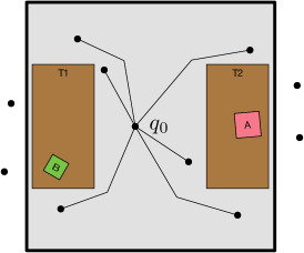
inline, color=blue!10, linecolor=blue!90, size=]TODO: I adopted a different convention for $\mathit{Manip}(x_{o},x_{o}^{\prime},x_{q},u_{m})$ than kin

Rather than specify ${\cal C}_{\mathit{Pick}}^{o}$ and ${\cal C}_{\mathit{Place}}^{o}$ transitions as instantaneous contacts with each object, we represent robot trajectories moving to, manipulating, and returning from an object as a single transition ${\cal C}_{\mathit{MPick}}^{o}$ or ${\cal C}_{\mathit{MPlace}}^{o}$.

$${\cal C}_{\mathit{MPick}}^{o}= \{\mathit{Stable}_{o},\mathit{Grasp}_{o}^{\prime},\mathit{Manip},$$

$$x_{h}=\textbf{None},x_{h}^{\prime}=o,\}\;\cup$$

$$\{x_{o^{\prime}}=x^{\prime}_{o^{\prime}},\mathit{CFree}_{o^{\prime}})\mid o^{\prime}\in{\cal O},o\neq o^{\prime}\}$$

$${\cal C}_{\mathit{MPlace}}^{o}= \{\mathit{Grasp}_{o},\mathit{Stable}_{o}^{\prime},\mathit{Manip}^{\prime},$$

$$x_{h}=o,x_{h}^{\prime}=\textbf{None}\}\;\cup$$

$$\{x_{o^{\prime}}=x^{\prime}_{o^{\prime}},\mathit{CFree}_{o^{\prime}}\mid o^{\prime}\in{\cal O},o\neq o^{\prime}\}$$

This behavior is enforced be a manipulation constraint $\mathit{Manip}$ on parameters $x_{o},x_{o}^{\prime},u_{m}$ representing poses $x_{o},x_{o}^{\prime}$ for object $o$ and trajectory $u_{m}$. Let $q_{0}$ be the initial robot configuration and $q_{\mathit{Kin}}$ be a kinematic solution for end-effector transform $x_{o}^{\prime}x_{o}^{-1}$ grasping object $o$ with grasp $x_{o}^{-1}$ at placement $x_{o}^{\prime}$. The trajectory $u_{m}$ is the concatenation of a motion plan from $q_{0}\to q_{\mathit{Kin}}$, a grasp plan, and a motion plan $q_{\mathit{Kin}}\to q_{0}$. Both motion plans are computed to be free of collisions with fixed obstacles. Additionally, one motion plan avoids collisions with $o$ placed at $x_{o}^{\prime}$, and the other avoids collisions between $o$ held at grasp $x_{o}$ and fixed obstacles. Because the robot always returns to $q_{0}$, the robot configuration need not be included as a state variable.

We structure the transition system this way based on the insight that the bulk of the robot’s configuration space is unaffected by the placements of movable obstacles. The moveable obstacles mostly only prevent the safe execution of manipulator trajectories above tabletops. Rather than directly plan paths between pairs of configurations manipulating objects, we instead plan paths to a home configuration chosen arbitrarily as the initial configuration $q_{0}$. This approach guarantees the feasibility of the resulting plan while not inducing significant overhead. Shorter, direct trajectories between pairs of base configurations can later be produced when post-processing a solution. Figure 17 visualizes the set of $u_{m}$ trajectories as edges in a star roadmap (Garrett et al., 2017a) with $q_{0}$ as the root.

inline, color=blue!10, linecolor=blue!90, size=]TODO: Placement instead of Stable or Pose

We specify the following samplers to produce values satisfying the constraints in this transition system. The grasp sampler $\psi_{P}^{o}$ and placement $\psi_{P}^{o}$ sampler are the same as before. The manipulation sampler $\psi_{M}^{o}$ is similar to $\psi_{IK}^{o}$:

$$\psi_{M}^{o}=\big{\langle}(x_{o},x_{o}^{\prime}),(u_{m}),\{\mathit{Manip}_{o}\},\textnormal{sample-manip}\big{\rangle}$$ .

The procedure sample-manip samples a nearby base pose via inverse reachability. From this base pose, it performs manipulator inverse kinematics to identify a grasping configuration to perform the pick or place. If sample-manip fails to find a kinematic solution, it samples a new base pose. Otherwise, it calls a sampling-based motion planner twice to find motion plans to this grasping configuration and back. These motion plans are computed to not be in collision with fixed obstacles or $o$ both when it is on the table and when it is held. Additionally, each call has a timeout meta parameter to ensure termination. The timeout for each sampler instance of $\psi_{M}^{o}$ is increased after each call allowing sample-manip to have an unbounded amount of time collectively over all of its calls.

inline, color=blue!10, linecolor=blue!90, size=]TODO: Correctness condition of planners using samplers?

10 Example Mobile Manipulation Problem

To illustrate both the incremental and focused algorithms, we work through their steps on an example mobile manipulation problem. Consider the problem in figure 16 with two movable objects $A,B$ and two tables $T1,T2$. States are $\bar{x}=(x_{A},x_{B},x_{h})$ and controls are $\bar{u}=u_{m}$. The initial state is $\bar{x}_{0}=(a_{0},b_{0},\textbf{None})$ and the goal constraints are ${\cal C}_{*}=\{\mathit{Region}_{A}\}$ indicating that object $A$ is placed on $T1$. For simplicity, we assume that each moveable object has a single grasp $a_{g}$ or $b_{g}$. The values $a_{0},b_{0},a_{g},b_{g}\in\text{SE}(3)$ represent continuous transformations. Similarly, manipulations $m$ are full body motion plans from $q_{0}$ to a grasping configuration and back. For the example, we assume that the conditional samplers never fail to produce an appropriate value.

10.1 Incremental Algorithm

Table 1 traces the sampler instances $S_{i}$ for which sample is called paired with the resulting element for each iteration $i$ of the incremental algorithm. The set of $\mathit{elements}$ available on each iteration is the union of the previously sampled elements $S_{j},j<i$. The incremental algorithm fails to find a plan for 2 iterations and finally finds the following plan $\pi_{3}$ on the 3rd iteration.

$$\vec{a}_{3} =[{\cal C}_{\mathit{MPick}}^{A},{\cal C}_{\mathit{MPlace}}^{A}]$$

$$\vec{x}_{3} =[(a_{0},b_{0},\textbf{None}),(a_{g},b_{0},A),(a_{1},b_{0},\textbf{None})]$$

$$\vec{u}_{3} =[m_{1},m_{3}]$$

Notice that the number of sampler instances sampled per iteration grows quickly. Additionally, samples are generated for both objects $A$ and $B$ despite the task only requiring manipulating $A$.

inline, color=blue!10, linecolor=blue!90, size=]TODO: Write the $\mathit{Var}$ or tests?

$S_{0}$	$\textnormal{initial-elements}({\cal P}):\{\mathit{Stable}(a_{0}),\mathit{Stable}(b_{0}))\}$
$\vec{a}_{1}$	None
$S_{1}$	$\psi_{G}^{a}():\mathit{Grasp}(a_{g}),\psi_{G}^{b}():\mathit{Grasp}(b_{g}),\psi_{P}^{A}():\mathit{Stable}(a_{1}),\psi_{P}^{B}():\mathit{Stable}(b_{1}),\mathit{Region}(a_{1})$
$\vec{a}_{2}$	None
$S_{2}$	$\psi_{M}^{A}(a_{0},a_{g}):\mathit{Manip}(a_{0},a_{g},m_{1}),\psi_{M}^{B}(b_{0},b_{g}):\mathit{Manip}(b_{0},b_{g},m_{2}),\psi_{M}^{A}(a_{1},a_{g}):\mathit{Manip}(a_{1},a_{g},m_{3}),$
	$\psi_{M}^{B}(b_{1},b_{g}):\mathit{Manip}(b_{1},b_{g},m_{4}),\psi_{P}^{A}():\mathit{Stable}(a_{2}),\psi_{P}^{B}():\mathit{Stable}(b_{2}),\mathit{Region}(a_{2})$
	$\mathit{CFree}(m_{1},b_{0}),\mathit{CFree}(m_{1},b_{1}),\mathit{CFree}(m_{1},b_{2}),\mathit{CFree}(m_{2},a_{0}),\mathit{CFree}(m_{2},a_{1}),\mathit{CFree}(m_{2},a_{2})$
$\vec{a}_{3}$	$\vec{a}_{3}=[{\cal C}_{\mathit{MPick}}^{A},{\cal C}_{\mathit{MPlace}}^{A}],\vec{x}_{3}=[(a_{0},b_{0},\textbf{None}),(a_{g},b_{0},A),(a_{1},b_{0},\textbf{None})],\vec{u}_{3}=[m_{1},m_{2}]$

Table 1: Example walkthrough of the incremental algorithm. Each $S_{i}$ displays the set of sampler instances for which sample is called along with the new elements produced.

10.2 Focused Example

Table 2 traces each iteration $i$ of the incremental algorithm. We will assume that $\mathit{new\_elements}$ are directly added to $\mathit{elements}$. As before, $S_{i}$ contains the sampler instances sample paired with the resulting elements. Elements certified by $\mathit{CFree}$ and $\mathit{Region}$ are individually added to $S_{i}$. The set of $\mathit{sampled}$ sampler instances are contained in $S_{j},i<j$. Let ${\cal E}_{i}$ be the set of elements using lazy samples generated by process-samplers on each iteration. The union of ${\cal E}_{i}$ and $\mathit{elements}$ is $\mathit{mixed\_elements}$. The plan returned on each iteration is denoted by $\pi_{i}=\langle\vec{a}_{i},\vec{x}_{i},\vec{u}_{i}\rangle$. We denote the lazy sampler for each sampler as follows:

$$\textnormal{lazy-sample}(\psi_{G}^{o}())=\{\mathit{Grasp}(l_{o}^{G})\}$$

$$\textnormal{lazy-sample}(\psi_{P}^{o}())=\{\mathit{Stable}(l_{o}^{P})\}$$

$$\textnormal{lazy-sample}(\psi_{M}^{o}(x_{o},x_{o}^{\prime}))=\{\mathit{Manip}(x_{o},x_{o}^{\prime},l_{m}^{o})\}$$

inline, color=blue!10, linecolor=blue!90, size=]TODO: If the only structure is a DAG, then you can avoid worrying about shared lazy or even having to move them to a lazy pool

inline, color=blue!10, linecolor=blue!90, size=]TODO: I could go back to using full samples

$S_{0}$	$\textnormal{initial-elements}({\cal P}):\{\mathit{Stable}(a_{0}),\mathit{Stable}(b_{0})\}$
${\cal E}_{1}$	$\mathit{Grasp}(l_{A}^{G}),\mathit{Grasp}(l_{B}^{G}),\mathit{Stable}(l_{A}^{P}),\mathit{Region}(l_{A}^{P}),\mathit{Stable}(l_{B}^{P}),\mathit{Manip}(a_{0},l_{A}^{G},l_{m}^{A}),\mathit{Manip}(b_{0},l_{B}^{G},l_{m}^{B}),$
	$\mathit{Manip}(l_{A}^{P},l_{A}^{G},l_{m}^{A}),\mathit{Manip}(l_{B}^{P},l_{B}^{G},l_{m}^{B}),\mathit{CFree}(l_{m}^{A},b_{0}),\mathit{CFree}(l_{m}^{A},l_{B}^{P}),\mathit{CFree}(l_{m}^{B},a_{0}),\mathit{CFree}(l_{m}^{B},l_{A}^{P})$
$\vec{\pi}_{1}$	$\vec{a}_{1}=[{\cal C}_{\mathit{MPick}}^{A},{\cal C}_{\mathit{MPlace}}^{A}],\vec{x}_{1}=[(a_{0},b_{0},\textbf{None}),(l_{A}^{G},b_{0},A),(l_{A}^{P},b_{0},\textbf{None})],\vec{u}_{1}=[l_{m}^{A},l_{m}^{A}]$
$S_{1}$	$\psi_{G}^{A}():\mathit{Grasp}(a_{g}),\psi_{P}^{A}():\mathit{Stable}(a_{1}),\mathit{Region}(a_{1})$
${\cal E}_{2}$	$\mathit{Grasp}(l_{B}^{G}),\mathit{Stable}(l_{B}^{P}),\mathit{Manip}(a_{0},a_{g},l_{m}^{A}),\mathit{Manip}(a_{1},a_{g},l_{m}^{A}),\mathit{CFree}(l_{m}^{A},b_{0}),\mathit{CFree}(l_{m}^{A},l_{B}^{P}),\mathit{CFree}(l_{m}^{B},a_{0}),$
	$\mathit{CFree}(l_{m}^{B},a_{1}),\mathit{Manip}(b_{0},l_{B}^{G},l_{m}^{B}),\mathit{Manip}(l_{B}^{P},l_{B}^{G},l_{m}^{B})$
$\vec{\pi}_{2}$	$\vec{a}_{2}=[{\cal C}_{\mathit{MPick}}^{A},{\cal C}_{\mathit{MPlace}}^{A}],\vec{x}_{2}=[(a_{0},b_{0},\textbf{None}),(a_{g},b_{0},A),(a_{1},b_{0},\textbf{None})],\vec{u}_{2}=[l_{m}^{A},l_{m}^{A}]$
$S_{2}$	$\psi_{M}^{A}(a_{0},a_{g}):\mathit{Manip}(a_{0},a_{g},m_{1}),\psi_{M}^{A}(a_{1},a_{g}):\mathit{Manip}(a_{1},a_{g},m_{2}),\mathit{CFree}(m_{1},p_{0}),\mathit{CFree}(m_{2},p_{0})$
${\cal E}_{3}$	$\mathit{Grasp}(l_{B}^{G}),\mathit{Stable}(l_{B}^{P}),\mathit{CFree}(m_{1},l_{B}^{P}),\mathit{CFree}(m_{2},l_{B}^{P}),\mathit{Manip}(b_{0},l_{B}^{G},l_{m}^{B})$
	$\mathit{Manip}(l_{B}^{P},l_{B}^{G},l_{m}^{B}),\mathit{CFree}(l_{m}^{B},a_{0}),\mathit{CFree}(l_{m}^{B},a_{1})$
$\vec{a}_{3}$	$\vec{a}_{3}=[{\cal C}_{\mathit{MPick}}^{A},{\cal C}_{\mathit{MPlace}}^{A}],\vec{x}_{3}=[(a_{0},b_{0},\textbf{None}),(a_{g},b_{0},A),(a_{1},b_{0},\textbf{None})],\vec{u}_{3}=[m_{1},m_{2}]$

Table 2: Example walkthrough of the focused algorithm. Each ${\cal E}_{i}$ displays the set of lazy elements at the start of the iteration. Each $S_{i}$ displays the set of sampler instances for which sample is called along with the new elements produced.

On the first iteration, the sampler instances $\psi_{G}^{a}(),\psi_{P}^{a}()$ are sampled to produce values for $l_{A}^{G},l_{A}^{P}$ respectively. On the second iteration, $\psi_{M}^{a}(a_{0},a_{g})$ and $\psi_{M}^{a}(a_{1},a_{g})$ generate the manipulations required for the ${\cal C}_{\mathit{MPick}}^{A}$ and ${\cal C}_{\mathit{MPlace}}^{A}$ transitions given the new grasp $a_{g}$ and placement $a_{1}$. On the final iteration, a plan $\pi_{3}$ not requiring any lazy samples is generated, resulting in a solution.

The focused algorithm samples fewer values than incremental by only sampling values determined to be useful for completing lazy samples and satisfying constraints along a plan. More specifically, it avoids sampling values for object $B$ altogether, saving time by not computing expensive motion plans. This behavior becomes even more prevalent in problems with many moveable objects, such as ones arising from human environments.

inline, color=blue!10, linecolor=blue!90, size=]TODO: Do I want to assume collision stuff is automatically produced?

inline, color=blue!10, linecolor=blue!90, size=]TODO: Add constraints to the sequence?

inline, color=blue!10, linecolor=blue!90, size=]TODO: Pose precondition on collision sampler

inline, color=blue!10, linecolor=blue!90, size=]TODO: Make the collision stuff right?

inline, color=blue!10, linecolor=blue!90, size=]TODO: Ensure the surface stuff is correct

inline, color=blue!10, linecolor=blue!90, size=]TODO: What if I just used computer output for these?

inline, color=blue!10, linecolor=blue!90, size=]TODO: What about the initial values here? How do I tell that they are poses?

10.3 Additional Example Scenarios

We sketch out several additional problems and outline how, in particular, the focused algorithm will proceed in each of these scenarios.

10.3.1 Sampling Failure:

We previously assumed that each sampler successfully generated output values satisfying its constraints. In general, samplers may fail to do so because of timeouts or even because no sample exists. For example, suppose $\psi_{M}^{A}(a_{0},a_{g})$ fails to produce a collision-free inverse kinematic solution, resulting in a failure. After the failure, $\psi_{M}^{A}(a_{0},a_{g})$ will be added to $\mathit{sampled}$, preventing it from being sampled on the next iteration. Without $\mathit{Manip}(a_{0},a_{g},m_{1})$ or $\mathit{Manip}(a_{0},a_{g},l_{m}^{A})$, the focused algorithm will fail to find a plan. In that case, $\mathit{sampled}$ is reset allowing $\psi_{M}^{A}(a_{0},a_{g})$ to be sampled again on the next episode. This cycle will automatically repeat with increased timeouts for as long as $\psi_{M}^{A}(a_{0},a_{g})$ fails to produce a manipulation, as picking object $A$ is required for any solution to this problem.

inline, color=blue!10, linecolor=blue!90, size=]TODO: Is the there exists a set of things with a set of successors that will admit a solution thing actually general?

10.3.2 Obstructions:

Suppose that object $A$ is initially obstructed by object $B$ as in figure 18. While $\psi_{M}^{A}(a_{0},a_{g})$ can produce a manipulation $m_{1}$, it cannot be performed because it violates the collision constraint $\mathit{CFree}(m_{1},b_{0})$. However, the lazy pose $l_{B}^{P}$ is optimistically assumed to not be in collision with $m_{1}$. Thus, a valid plan involves first moving $B$ to $l_{B}^{P}$ before picking $A$. In the event where the sampled value for $l_{B}^{P}$ is still in collision with $m_{1}$, an additional value can be generated on the next episode. Lazy samples allow the focused algorithm to reason about trajectories $u_{m}$ that do not yet correspond to a feasible transition because they violate one or more collision constraints. By sampling concrete values for the lazy samples corresponding to these violated constraints, it can attempt to find transitions for which the control is feasible.

Figure 18: Mobile manipulation problem where object $B$ is obstructing manipulations that pick object $A$.

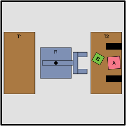
10.3.3 Regrasp:

Consider the regrasp experiment in figure 23 where the robot is unable to pick and place the goal object using the same grasp. Because of this, it is forced to place the goal object at an intermediate location to change grasps. The focused algorithm will only create one lazy grasp sample $l_{A}^{G}$ for object $A$. On the subsequent iteration, at least one of $\psi_{M}^{A}(a_{0},a_{g})$ and $\psi_{M}^{A}(a_{*},a_{g})$ will fail to sample a manipulation. Both will be added to $\mathit{sampled}$ causing the discrete-search to fail to find a plan on the next iteration. After $\mathit{sampled}$ is reset, the focused algorithm is able to use $l_{A}^{G}$ to produce the second grasp and arrive at a solution to the problem.

11 Experiments

We implemented both algorithms and tested them on a suite of tabletop manipulation problems. All experiments used the same core factored transition system and same set of conditional samplers as those described in section 9. We wrote our conditional samplers in Python, building on top of the OpenRAVE robotics development environment (Diankov and Kuffner, 2008). We used the Open Dynamics Engine (Smith, 2005) for collision checking.

Each movable object was limited to four side-grasps except for in Experiment 1 where each object has a single-top grasp. Thus, the grasp conditional sampler $\psi_{G}$ simply enumerates this finite set. The side-grasp restriction increases the difficulty of our benchmarks as it creates more opportunities for objects to obstruct each other.

Our placement conditional sampler $\psi_{P}$ randomly samples poses from a mixture distribution composed of a uniform distribution over stable placements and a uniform distribution over stable placements not in collision given the initial state. This strong bias towards initially collision-free placements accelerates the generation of unobstructed placements, particularly in problems where there are many movable objects.

Our manipulation conditional sampler $\psi_{M}$ samples base poses from a precomputed distribution of 2D base poses, each relative to a 2D object pose, that for some previous query admitted a kinematic solution. This “learned” base pose sampler has a greater likelihood of producing base poses that admit kinematic solutions than a sampler that generates base poses uniformly at random in a region near the desired end-effector pose. We use IKFast (Diankov, 2010) for inverse kinematics. Finally, we implemented $\psi_{M}$’s sampling-based motion planner using RRT-Connect (Bidirectional Rapidly-exploring Randomized Trees) (Kuffner and LaValle, 2000).

We considered two FastDownward (Helmert, 2006) configurations for the incremental and focused algorithms: H uses the FastForward heuristic (Hoffmann and Nebel, 2001) in a lazy greedy search and No-H is a breadth-first search.

All trials were run on 2.8 GHz Intel Core i7 processor with a 120 second time limit. Our Python implementation of the incremental and focused algorithms can be found here: https://github.com/caelan/factored-transition-systems. We also have developed a similar suite of algorithms for an extension of the PDDL (McDermott et al., 1998) called STRIPStream (Garrett et al., 2017b) available at https://github.com/caelan/stripstream. Videos of the experiments are available at https://youtu.be/xJ3OeMAYmgc. Base trajectories are post-processed by computing a direct trajectory between pairs of base configurations.

11.1 Scaling Experiments

We performed three scaling experiments on pick-and-place problems. All experiments considered five problem sizes, varying the number of objects. We performed five trials using randomly (with the exception of Experiment 2) generated problem instances for each problem size. Each scatter plot in figures 19, 21, and 22 display the total runtime of each configuration per trial. Timeouts are indicated by the omission of a trial.

Figure 19: Experiment 1: total runtime of the algorithms over 5 trials per problem size.

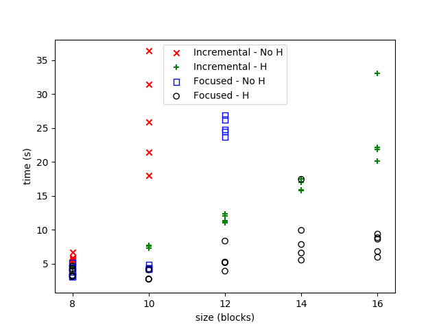
Experiment 1 in figure 1 is the “grid@tabletop” benchmark (Krontiris and Bekris, 2015) where each object has a specified goal pose. The initial placements are randomly generated. The table size scales with the number of objects. As shown in figure 19, Focused-H solved all problem instances and Incremental-H solved all but one (size=14) indicating that use of a heuristic is necessary for problems with long-horizons.

Figure 20: Experiment 2: the robot must place the green object in the green region.

Figure 21: Experiment 2: total runtime of the algorithms over 5 trials per problem size.

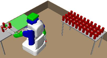
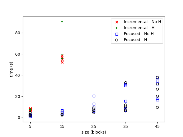
Experiment 2 in figure 20 has the goal that a single green object be placed in the green region. The green object is obstructed by four red objects. The number of distracting red objects on the right table is varied between 0 and 40. This experiment reflects many real-world environments where the state-space is enormous but many objects do not substantially affect a task. As can be seen in figure 21, both Focused-No-H and Focused-H solved all problem instances showing that the focused algorithm is able to avoid producing samples for objects until they are relevant to the task.

Figure 22: Experiment 3: total runtime of the algorithms over 5 trials per problem size.

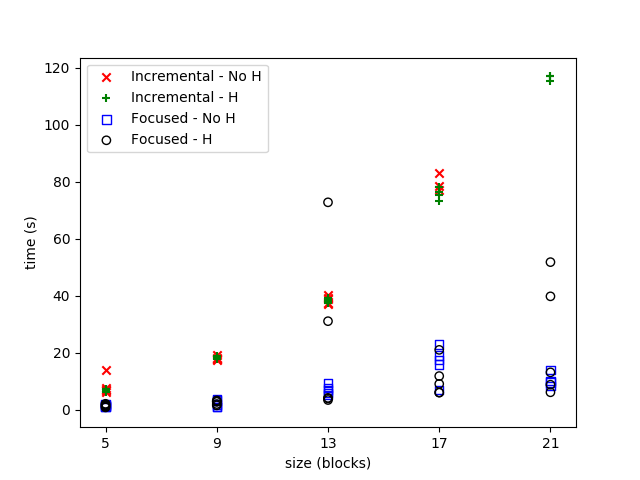
Experiment 3 in figure 1 has the goal that a single blue object be moved to a different table. The blue object starts at the center of the visible table, and the red objects are randomly placed on the table. The table size scales with the number of objects. As shown in figure 22, Focused-H solved all instances and Focused-No-H solved all but one (size=21).

11.2 Diverse Experiments

We experimented on several additional problems to show that the factored transition system framework and algorithms can be successfully applied to problems involving pushing, stacking, and discrete state variables. We also experimented on two tricky pick-and-place problems that require regrasping and require violating several goal constraints along a plan to achieve the goal. We conducted 40 trials per problem and algorithm, and each trial once again had a 120 second time limit. The success percentage of each algorithm (%) and mean runtime in seconds for successful trials are displayed in table 3. We also show the reported statistics for the best configuration of the HBF Garrett et al. (2015) and FFRob Garrett et al. (2017a) algorithms when applicable.

11.2.1 Descriptions

The regrasp problem (Regrasp) in figure 23 is Problem 3 of Garrett et al. (2015). The goal constraints are that the green object be at the green pose and the blue object remain at its current pose. The robot must place the green object at an intermediate pose to obtain a new grasp in order to insert it in the thin, right cupboard. This indicates that the algorithms can solve pick-and-place problems where even non-collision constraints affect the plan skeleton of solutions.

The first pushing problem (Push) in figure 23 has the goal constraint that the short blue cylinder on the left table be placed at the blue point on the right table. Because the blue cylinder is short and wide, the robot is unable to grasp it except by side grasps at the edges of each table. Thus, the robot must first push the cylinder to the edge of the left table, pick the cylinder, place the cylinder on the edge of the right table, and push the cylinder to the goal point. This problem introduces an additional transition relating to trajectories corresponding movements between two poses. Additionally, it requires a conditional sampler to generate push Cartesian trajectories and motion plans per pairs of poses on the same table.

Figure 23: Regrasp (left): a forced regrasp problem. Push (right): a problem requiring pushing, picking, and placing.

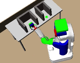
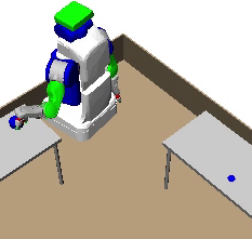
The second pushing problem (Wall) in figure 24 is Problem 2 of Garrett et al. (2015) where the goal constraint is that the short green cylinder be placed at the green point. A wall of moveable objects initially blocks the robot from pushing the the green cylinder to the goal point. However, if several of these blocks are moved, the robot can execute a sequence of pushes to push the green cylinder directly to its goal.

Figure 24: Wall: a pushing problem involving a wall of blocks.

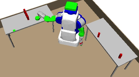
The stacking problem (Stacking) in figure 25 is Problem 4 of Garrett et al. (2015). The goal constraints are that the blue block be contained within the blue region, the green block be contained within the green region, and the black block be on top of the blue block. The robot must unstack the red block to safely move the green block. This problem requires a modification of the transition system to account for stability constraints. Additionally, it requires a conditional sampler that produces poses of the black block on the blue block given poses of the blue block.

Figure 25: Stacking: a problem requiring unstacking and stacking.

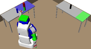
The pick-and-place problem (Nonmon.) in figure 26 is Problem 3-2 of Garrett et al. (2017a). The goal constraints are that the green blocks be moved from their initial pose on the left table to their corresponding pose on the right table. Additionally, there are goal constraints that each blue and cyan block end at its initial pose. This is a highly nonmonotonic problem as solutions require violating several goal constraints satisfied by the initial state.

Figure 26: Nonmon.: a nonmonotonic pick-and-place problem.

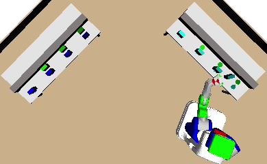
The task and motion planning problem (Dinner) in figure 27 is Problem 5 of Garrett et al. (2017a). The state contains an additional discrete state variable for each block indicating whether it is dirty, clean, or cooked. The transition relation contains additional clauses to clean a dirty block when it is placed on the dishwasher and to cook a clean block when it is placed on the microwave. The goal constraints are that the green blocks (“cabbage”) be cooked and placed on the plates, the blue blocks (“cups”) be cleaned and placed at the blue points, the cyan block (an unnecessary “cup”) be cleaned, and the pink blocks (“turnips”) remain placed on the shelf. To reach the cabbage, the robot must first move several turnips and the later replace them to keep the kitchen tidy.

11.2.2 Results

Each algorithm performed comparably on the first four problems (Regrasp, Push, Wall, Stacking). When compared to HBF (Garrett et al., 2015), Focused-H has a slightly lower average runtime for Regrasp and Stacking and about the same average runtime for Wall. However, the average runtime for all algorithms on these problems is less than 15 seconds. Only the heuristically informed algorithms where able to consistently solve the larger last two problems (Nonmon., Dinner). For problem Nonmon., Incremental-H slightly outperformed Focused-H because this problem requires manipulating each object. Thus, Incremental-H and Focused-H produce comparable sets of samples, but Incremental-H has less overhead. Both algorithms performed significantly better than best algorithm of Garrett et al. (2017a). For problem Dinner, the heuristic guided Incremental-H and Focused-H planners were able to quickly solve the problem reinforcing the point that search guidance is necessary for problems over long horizons. These algorithms compare favorably to the best algorithm of Garrett et al. (2017a).

Figure 27: Dinner: a task and motion planning problem.

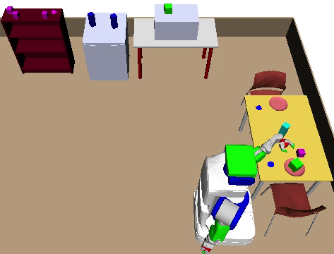
	HBF (2015)		FFRob (2017)		Incr.		Incr. - H		Focus		Focus - H
Problem	%	t	%	t	%	t	%	t	%	t	%	t
Regrasp	100	6	-	-	98	1	100	2	98	1	95	1
Push	-	-	-	-	100	11	100	13	100	13	100	9
Wall	100	7	-	-	95	10	98	13	100	6	100	8
Stacking	97	12	-	-	100	9	100	9	100	2	100	3
Nonmon.	-	-	72	135	25	21	98	15	0	-	88	43
Dinner	-	-	74	44	0	-	100	27	0	-	98	22

Table 3: The success percentage (%) and mean runtime in seconds (t) for the diverse experiments over 40 trials compared to the reported results for the HBF (Garrett et al., 2015) and FFRob (Garrett et al., 2017a) algorithms. A dash (-) indicates that no data was available.

inline, color=blue!10, linecolor=blue!90, size=]TODO: Motion, multi-goal motion, 2D pick-and-place

inline, color=blue!10, linecolor=blue!90, size=]TODO: Set a random seed per sampler and compare plan to the best possible one

12 Conclusion

We introduced factored transition systems for specifying planning problems in discrete-time hybrid systems. Factored transition systems can model motion planning, pick-and-place planning, and task and motion planning applications. The transition dynamics for multi-object manipulation are significantly factorable. Legal transitions can be expressed as the conjunction of constraints each involving only several state or control variables.

Conditional constraint manifolds enabled us to give a general definition of robust feasibility for factored transition systems. Under certain conditions, they allow us to describe a submanifold of plan parameter-space resulting from the intersection of dimensionality-reducing constraints. Thus, robustness properties can be examined relative to this submanifold rather than the for plan parameter-space. We introduced the idea of conditional samplers: samplers that given input values, produce a sequence of output values satisfying a constraint with the input values. When appropriate conditional samplers are specified for each conditional constraint manifold, the resulting collection of samplers is sufficient for solving any robustly feasible problem. Sampling benefits from factoring because a small collection of samples for each variable can correspond to a large number of combined states and transitions.

We gave two general-purpose algorithms that are probabilistically complete given sufficient samplers. The incremental algorithm iteratively calls each conditional sampler and tests whether the set of samples is sufficient using a blackbox, discrete search. The focused algorithm first creates lazy samples representing hypothetical outputs of conditional samplers and then uses a blackbox, discrete search to identify which lazy samples could be useful. We empirically demonstrated that these algorithms are effective at solving challenging pick-and-place, pushing, and task and motion planning problems. The focused algorithm is more effective than the incremental algorithm in problems with many movable objects as it can selectively produce samples for only objects affecting the feasibility of a solution. Additionally, both algorithms were more efficient when using a discrete search subroutine that exploited factoring in the search through domain-independent heuristics.

12.1 Future Work

Future work involves developing additional algorithms for solving factored transition systems. In particular, both the incremental and focused algorithms treat discrete-search as a blackbox. By directly integrating the search and sampling, an algorithm may be able to more directly target sampling based on the search state and possible transitions. For example, Backward-Forward Search (Garrett et al., 2015) performs its search directly in the hybrid state-space instead of a discretized state-space.

Our formulation gives rise to several new opportunities for learning to improve sampling and search runtimes. For instance, one could learn a policy to decide how frequently to sample each conditional sampler. A high performing policy would balance the likelihood of a conditional sampler to produce useful samples, the overhead of computing samples, and the impact additional samples have on subsequent discrete searches. Similarly, in the focused algorithm, one could learn costs associated with using lazy samples reflective of the expected future planning time resulting from sampling from a particular conditional stream. These costs could cause discrete-search to produce plans that are likely realizable without too much overhead.

Finally, this work can be extended to optimal planning settings where there are nonnegative costs $c(\bar{u})$ on control inputs. This will require adapting properties such as asymptotic optimality (Karaman and Frazzoli, 2011) to the factored transition system setting and modifying the incremental and focused algorithms to achieve these properties.

13 Acknowledgements

We thank Beomjoon Kim, Ferran Alet, and Zi Wang for their feedback on this manuscript. We gratefully acknowledge support from NSF grants 1420316, 1523767 and 1723381, from AFOSR FA9550-17-1-0165, from ONR grant N00014-14-1-0486. Caelan Garrett is supported by an NSF GRFP fellowship with primary award number 1122374. Any opinions, findings, and conclusions or recommendations expressed in this material are those of the authors and do not necessarily reflect the views of our sponsors.

References

- Alami et al. (1994) Alami R, Laumond JP and Siméon T (1994) Two manipulation planning algorithms. In: Workshop on Algorithmic Foundations of Robotics (WAFR). URL http://dl.acm.org/citation.cfm?id=215085.
- Alami et al. (1990) Alami R, Siméon T and Laumond JP (1990) A geometrical approach to planning manipulation tasks. the case of discrete placements and grasps. In: International Symposium of Robotic Research (ISRR). URL http://dl.acm.org/citation.cfm?id=112736.
- Alur et al. (1995) Alur R, Courcoubetis C, Halbwachs N, Henzinger TA, Ho PH, Nicollin X, Olivero A, Sifakis J and Yovine S (1995) The algorithmic analysis of hybrid systems. Theoretical computer science 138(1): 3–34.
- Alur et al. (2000) Alur R, Henzinger TA, Lafferriere G and Pappas GJ (2000) Discrete abstractions of hybrid systems. Proceedings of the IEEE 88(7): 971–984.
- Bäckström and Nebel (1995) Bäckström C and Nebel B (1995) Complexity results for SAS+ planning. Computational Intelligence 11(4): 625–655.
- Barraquand et al. (1997) Barraquand J, Kavraki L, Latombe JC, Motwani R, Li TY and Raghavan P (1997) A random sampling scheme for path planning. International Journal of Robotics Research (IJRR) 16(6): 759–774.
- Barry et al. (2013) Barry J, Kaelbling LP and Lozano-Pérez T (2013) A hierarchical approach to manipulation with diverse actions. In: Robotics and Automation (ICRA), 2013 IEEE International Conference on. IEEE, pp. 1799–1806. URL http://citeseerx.ist.psu.edu/viewdoc/summary?doi=10.1.1.365.1060.
- Barry (2013) Barry JL (2013) Manipulation with diverse actions. PhD Thesis, Massachusetts Institute of Technology.
- Berenson and Srinivasa (2010) Berenson D and Srinivasa SS (2010) Probabilistically complete planning with end-effector pose constraints. In: Robotics and Automation (ICRA), 2010 IEEE International Conference on. IEEE, pp. 2724–2730.
- Bohlin and Kavraki (2000) Bohlin R and Kavraki LE (2000) Path planning using lazy PRM. In: IEEE International Conference on Robotics and Automation (ICRA), volume 1. IEEE, pp. 521–528. URL http://ieeexplore.ieee.org/document/844107/.
- Bonet and Geffner (2001) Bonet B and Geffner H (2001) Planning as heuristic search. Artificial Intelligence 129(1): 5–33.
- Cambon et al. (2009) Cambon S, Alami R and Gravot F (2009) A hybrid approach to intricate motion, manipulation and task planning. International Journal of Robotics Research (IJRR) 28. URL http://journals.sagepub.com/doi/abs/10.1177/0278364908097884.
- Dantam et al. (2016) Dantam NT, Kingston Z, Chaudhuri S and Kavraki LE (2016) Incremental task and motion planning: A constraint-based approach. In: Robotics: Science and Systems (RSS). URL http://www.roboticsproceedings.org/rss12/p02.pdf.
- de Silva et al. (2013) de Silva L, Pandey AK, Gharbi M and Alami R (2013) Towards combining HTN planning and geometric task planning. In: RSS Workshop on Combined Robot Motion Planning and AI Planning for Practical Applications. URL https://arxiv.org/abs/1307.1482.
- Dechter (1992) Dechter R (1992) Constraint networks. Technical report, Information and Computer Science, University of California, Irvine. URL http://www.ics.uci.edu/~csp/r17-survey.pdf.
- Dellin and Srinivasa (2016) Dellin CM and Srinivasa SS (2016) A unifying formalism for shortest path problems with expensive edge evaluations via lazy best-first search over paths with edge selectors. International Conference on Automated Planning and Scheduling (ICAPS) URL https://arxiv.org/abs/1603.03490.
- Deshpande et al. (2016) Deshpande A, Kaelbling LP and Lozano-P?erez T (2016) Decidability of semi-holonomic prehensile task and motion planning. Workshop on Algorithmic Foundations of Robotics (WAFR) URL http://lis.csail.mit.edu/pubs/deshpande-WAFR16.pdf.
- Diankov (2010) Diankov R (2010) Automated construction of robotic manipulation programs. PhD Thesis, Robotics Institute, Carnegie Mellon University.
- Diankov and Kuffner (2008) Diankov R and Kuffner J (2008) Openrave: A planning architecture for autonomous robotics. Technical Report CMU-RI-TR-08-34, Robotics Institute, Carnegie Mellon University. URL https://pdfs.semanticscholar.org/c28d/3dc33b629916a306cc58cbff05dcd632d42d.pdf.
- Dornhege et al. (2009) Dornhege C, Eyerich P, Keller T, Trüg S, Brenner M and Nebel B (2009) Semantic attachments for domain-independent planning systems. In: International Conference on Automated Planning and Scheduling (ICAPS). AAAI Press, pp. 114–121. URL https://www.aaai.org/ocs/index.php/ICAPS/ICAPS09/paper/viewPaper/754.
- Dornhege et al. (2013) Dornhege C, Hertle A and Nebel B (2013) Lazy evaluation and subsumption caching for search-based integrated task and motion planning. In: IEEE/RSJ International Conference on Intelligent Robots and Systems (IROS) Workshop on AI-based robotics. URL https://robohow.eu/_media/workshops/ai-based-robotics-iros-2013/paper08-final.pdf.
- Edelkamp (2004) Edelkamp S (2004) Pddl2.2: The language for the classical part of the 4th international planning competition. 4th International Planning Competition (IPC’04), at ICAPS’04. URL https://pdfs.semanticscholar.org/4b3c/0706d2673d817cc7c33e580858e65b134ba2.pdf.
- Erdem et al. (2011) Erdem E, Haspalamutgil K, Palaz C, Patoglu V and Uras T (2011) Combining high-level causal reasoning with low-level geometric reasoning and motion planning for robotic manipulation. In: IEEE International Conference on Robotics and Automation (ICRA).
- Erol et al. (1994) Erol K, Hendler J and Nau DS (1994) Htn planning: Complexity and expressivity. In: AAAI, volume 94. pp. 1123–1128.
- Fikes and Nilsson (1971) Fikes RE and Nilsson NJ (1971) STRIPS: A new approach to the application of theorem proving to problem solving. Artificial Intelligence 2: 189–208.
- Garrett et al. (2014) Garrett CR, Lozano-Pérez T and Kaelbling LP (2014) FFRob: An efficient heuristic for task and motion planning. In: Workshop on the Algorithmic Foundations of Robotics (WAFR). URL https://link.springer.com/chapter/10.1007%2F978-3-319-16595-0_11.
- Garrett et al. (2015) Garrett CR, Lozano-Pérez T and Kaelbling LP (2015) Backward-forward search for manipulation planning. In: IEEE/RSJ International Conference on Intelligent Robots and Systems (IROS). URL http://lis.csail.mit.edu/pubs/garrett-iros15.pdf.
- Garrett et al. (2017a) Garrett CR, Lozano-Perez T and Kaelbling LP (2017a) Ffrob: Leveraging symbolic planning for efficient task and motion planning. The International Journal of Robotics Research 10.1177/0278364917739114. URL https://arxiv.org/abs/1608.01335.
- Garrett et al. (2017b) Garrett CR, Lozano-Pérez T and Kaelbling LP (2017b) Strips planning in infinite domains. arXiv preprint arXiv:1701.00287 .
- Hauser and Latombe (2010) Hauser K and Latombe JC (2010) Multi-modal motion planning in non-expansive spaces. International Journal of Robotics Research (IJRR) 29: 897–915.
- Hauser and Ng-Thow-Hing (2011) Hauser K and Ng-Thow-Hing V (2011) Randomized multi-modal motion planning for a humanoid robot manipulation task. International Journal of Robotics Research (IJRR) 30(6): 676–698. URL http://journals.sagepub.com/doi/abs/10.1177/0278364910386985.
- Helmert (2006) Helmert M (2006) The fast downward planning system. Journal of Artificial Intelligence Research (JAIR) 26: 191–246. URL http://www.jair.org/papers/paper1705.html.
- Henzinger (2000) Henzinger TA (2000) The theory of hybrid automata. In: Verification of Digital and Hybrid Systems. Springer, pp. 265–292.
- Hoffmann and Nebel (2001) Hoffmann J and Nebel B (2001) The FF planning system: Fast plan generation through heuristic search. Journal Artificial Intelligence Research (JAIR) 14: 253–302. URL http://dl.acm.org/citation.cfm?id=1622404.
- Hsu et al. (1997) Hsu D, Latombe JC and Motwani R (1997) Path planning in expansive configuration spaces. In: Robotics and Automation, 1997. Proceedings., 1997 IEEE International Conference on, volume 3. IEEE, pp. 2719–2726.
- Jensen (1996) Jensen FV (1996) An introduction to Bayesian networks, volume 210. UCL press London.
- Kaelbling and Lozano-Pérez (2011) Kaelbling LP and Lozano-Pérez T (2011) Hierarchical planning in the now. In: IEEE International Conference on Robotics and Automation (ICRA). URL http://ieeexplore.ieee.org/document/5980391/.
- Karaman and Frazzoli (2011) Karaman S and Frazzoli E (2011) Sampling-based algorithms for optimal motion planning. The International Journal of Robotics Research 30(7): 846–894.
- Kavraki et al. (1998) Kavraki LE, Kolountzakis MN and Latombe JC (1998) Analysis of probabilistic roadmaps for path planning. Robotics and Automation, IEEE Transactions on 14(1): 166–171.
- Kavraki and Latombe (1998) Kavraki LE and Latombe JC (1998) Probabilistic roadmaps for robot path planning. Practical Motion Planning in Robotics: Current Approaches and Future Directions .
- Kavraki et al. (1995) Kavraki LE, Latombe JC, Motwani R and Raghavan P (1995) Randomized query processing in robot path planning. In: Proceedings of the twenty-seventh annual ACM symposium on Theory of computing. ACM, pp. 353–362.
- Kavraki et al. (1996) Kavraki LE, Svestka P, Latombe JC and Overmars MH (1996) Probabilistic roadmaps for path planning in high-dimensional configuration spaces. IEEE Transactions on Robotics and Automation 12(4): 566–580. URL http://ieeexplore.ieee.org/document/508439/.
- Krontiris and Bekris (2015) Krontiris A and Bekris KE (2015) Dealing with difficult instances of object rearrangement. In: Robotics: Science and Systems (RSS). Rome, Italy. URL http://www.cs.rutgers.edu/~kb572/pubs/Krontiris_Bekris_rearrangement_RSS2015.pdf.
- Krontiris and Bekris (2016) Krontiris A and Bekris KE (2016) Efficiently solving general rearrangement tasks: A fast extension primitive for an incremental sampling-based planner. In: International Conference on Robotics and Automation (ICRA). Stockholm, Sweden. URL http://www.cs.rutgers.edu/~kb572/pubs/fast_object_rearrangement.pdf.
- Kuffner and LaValle (2000) Kuffner JJ Jr and LaValle SM (2000) RRT-Connect: An efficient approach to single-query path planning. In: IEEE International Conference on Robotics and Automation (ICRA).
- Lagriffoul et al. (2014) Lagriffoul F, Dimitrov D, Bidot J, Saffiotti A and Karlsson L (2014) Efficiently combining task and motion planning using geometric constraints. International Journal of Robotics Research (IJRR) : 0278364914545811URL http://journals.sagepub.com/doi/abs/10.1177/0278364914545811?journalCode=ijra.
- Lagriffoul et al. (2012) Lagriffoul F, Dimitrov D, Saffiotti A and Karlsson L (2012) Constraint propagation on interval bounds for dealing with geometric backtracking. In: IEEE/RSJ International Conference on Intelligent Robots and Systems (IROS). URL http://ieeexplore.ieee.org/document/6385972/.
- Laumond (1998) Laumond JPP (1998) Robot Motion Planning and Control. Secaucus, NJ, USA: Springer-Verlag New York, Inc. ISBN 3540762191.
- LaValle (2006) LaValle SM (2006) Planning Algorithms. Cambridge University Press. URL msl.cs.uiuc.edu/planning.
- Lozano-Pérez (1981) Lozano-Pérez T (1981) Automatic planning of manipulator transfer movements. IEEE Transactions on Systems, Man, and Cybernetics 11: 681–698. URL http://ieeexplore.ieee.org/document/4308589/.
- Lozano-Pérez et al. (1987) Lozano-Pérez T, Jones JL, Mazer E, O’Donnell PA, Grimson WEL, Tournassoud P and Lanusse A (1987) Handey: A robot system that recognizes, plans, and manipulates. In: IEEE International Conference on Robotics and Automation (ICRA). URL http://ieeexplore.ieee.org/document/1087847/.
- Lozano-Pérez and Kaelbling (2014) Lozano-Pérez T and Kaelbling LP (2014) A constraint-based method for solving sequential manipulation planning problems. In: IEEE/RSJ International Conference on Intelligent Robots and Systems (IROS). IEEE, pp. 3684–3691. URL http://lis.csail.mit.edu/pubs/tlpk-iros14.pdf.
- McDermott et al. (1998) McDermott D, Ghallab M, Howe A, Knoblock C, Ram A, Veloso M, Weld D and Wilkins D (1998) Pddl: The planning domain definition language. Technical report, Yale Center for Computational Vision and Control. URL http://citeseerx.ist.psu.edu/viewdoc/summary?doi=10.1.1.51.9941.
- Pandey et al. (2012) Pandey AK, Saut JP, Sidobre D and Alami R (2012) Towards planning human-robot interactive manipulation tasks: Task dependent and human oriented autonomous selection of grasp and placement. In: RAS/EMBS International Conference on Biomedical Robotics and Biomechatronics. URL http://ieeexplore.ieee.org/abstract/document/6290776/.
- Plaku and Hager (2010) Plaku E and Hager G (2010) Sampling-based motion planning with symbolic, geometric, and differential constraints. In: IEEE International Conference on Robotics and Automation (ICRA). URL http://ieeexplore.ieee.org/document/5509563/.
- Siméon et al. (2004) Siméon T, Laumond JP, Cortés J and Sahbani A (2004) Manipulation planning with probabilistic roadmaps. International Journal of Robotics Research (IJRR) 23(7-8): 729–746. URL http://journals.sagepub.com/doi/abs/10.1177/0278364904045471.
- Smith (2005) Smith R (2005) Open dynamics engine.
- Srivastava et al. (2014) Srivastava S, Fang E, Riano L, Chitnis R, Russell S and Abbeel P (2014) Combined task and motion planning through an extensible planner-independent interface layer. In: IEEE International Conference on Robotics and Automation (ICRA). URL http://ieeexplore.ieee.org/document/6906922/.
- Stilman and Kuffner (2006) Stilman M and Kuffner JJ (2006) Planning among movable obstacles with artificial constraints. In: Workshop on Algorithmic Foundations of Robotics (WAFR).
- Stilman et al. (2007) Stilman M, Schamburek JU, Kuffner JJ and Asfour T (2007) Manipulation planning among movable obstacles. In: IEEE International Conference on Robotics and Automation (ICRA). URL http://ieeexplore.ieee.org/document/4209604/.
- Thiébaux et al. (2005) Thiébaux S, Hoffmann J and Nebel B (2005) In defense of pddl axioms. Artificial Intelligence 168(1-2): 38–69.
- Torrisi and Bemporad (2001) Torrisi FD and Bemporad A (2001) Discrete-time hybrid modeling and verification. In: Proc. 40th IEEE Conf. on Decision and Control, volume 3. IEEE, pp. 2899–2904.
- Toussaint (2015) Toussaint M (2015) Logic-geometric programming: an optimization-based approach to combined task and motion planning. In: AAAI Conference on Artificial Intelligence. AAAI Press, pp. 1930–1936. URL https://www.ijcai.org/Proceedings/15/Papers/274.pdf.
- Toussaint and Lopes (2017) Toussaint M and Lopes M (2017) Multi-bound tree search for logic-geometric programming in cooperative manipulation domains. In: Robotics and Automation (ICRA), 2017 IEEE International Conference on. IEEE, pp. 4044–4051.
- Tu (2010) Tu LW (2010) An Introduction to Manifolds. Springer. URL http://www.springer.com/gp/book/9781441973993.
- Van Den Berg et al. (2009) Van Den Berg J, Stilman M, Kuffner J, Lin M and Manocha D (2009) Path planning among movable obstacles: a probabilistically complete approach. In: Algorithmic Foundation of Robotics VIII. Springer, pp. 599–614. URL https://link.springer.com/chapter/10.1007%2F978-3-642-00312-7_37.
- Vega-Brown and Roy (2016) Vega-Brown W and Roy N (2016) Asymptotically optimal planning under piecewise-analytic constraints. In: Workshop on the Algorithmic Foundations of Robotics (WAFR). URL http://www.wafr.org/papers/WAFR_2016_paper_11.pdf.
- Vendittelli et al. (2015) Vendittelli M, Laumond JP and Mishra B (2015) Decidability of robot manipulation planning: Three disks in the plane. In: Algorithmic Foundations of Robotics XI. Springer, pp. 641–657.
- Wilfong (1988) Wilfong GT (1988) Motion planning in the presence of movable obstacles. In: Symposium on Computational Geometry. pp. 279–288. URL https://link.springer.com/article/10.1007/BF01530890.