IHT dies hard: Provable convergence for accelerated Iterative Hard Thresholding

Rajiv Khanna and Anastasios Kyrillidis
University of Texas at Austin
IBM T.J. Watson Research Center
Abstract.

We study –both in theory and practice– the use of momentum in classic iterative hard thresholding (IHT) methods. By simply modifying classical IHT, we investigate its convergence behavior on convex optimization criteria with non-convex constraints, under standard assumptions. We observe that acceleration in IHT leads to significant improvements, compared to state of the art projected gradient descent and Frank-Wolfe variants. As a byproduct of our inspection, we study the impact of selecting the momentum parameter: similar to convex settings, two modes of behavior are observed –“rippling” and linear– depending on the level of momentum.

(Improved version based on comments from peer-review process; removed assumptions on optimal point; noisy case included)

1. Introduction

It is a well-known fact in convex optimization that momentum techniques provably result into significant gains w.r.t. convergence rate. Since 1983, when Nesterov proposed his optimal gradient methods [1], these techniques have been used in diverse machine learning and signal processing tasks. Lately, the use of momentum has re-gained popularity in non-convex settings, thanks to their improved performance in structured practical scenaria: from empirical risk minimization (ERM) to training neural networks.

Here, we mainly focus on structured constrained ERM optimization problems:

(1) minimizexn𝑥superscript𝑛minimize\displaystyle\underset{x\in\mathbb{R}^{n}}{\text{minimize}} f(x)(:=12bΦx22)annotated𝑓𝑥assignabsent12superscriptsubscriptnorm𝑏Φ𝑥22\displaystyle f(x)\left(:=\tfrac{1}{2}\|b-\Phi x\|_{2}^{2}\right) subject to x𝒞,𝑥𝒞\displaystyle x\in\mathcal{C},

that involve convex objectives f𝑓f and simple structured, but non-convex, constraints 𝒞𝒞\mathcal{C}, that can be described using a set of atoms, as in [2, 3]; see also Section 2.1. We note that our theory goes beyond the vector least squares case, with applications also in low-rank recovery.

Practical algorithms for (1) are convexified projected gradient descent schemes [3], non-convex iterative hard thresholding (IHT) variants [4] and Frank-Wolfe (FW) methods [5]. Convex methods can accommodate acceleration due to [1, 6] and come with rigorous theoretical guarantees; but, higher computational complexity might be observed in practice (depending on the nature of 𝒞𝒞\mathcal{C}); further, their configuration could be harder and/or non-intuitive. FW variants [7, 8] simplify the handling of constraints, but the successive construction of estimates –by adding singleton atoms to the putative solution– could slow down convergence. Non-convex methods, such as IHT [9, 10], could be the methods of choice in practice, but only few schemes justify their behavior in theory. Even more importantly, IHT schemes that utilize acceleration inferably are lacking. We defer the discussion on related work to Section 5.

In this work, we study the use of acceleration in IHT settings and supply additional information about open questions regarding the convergence and practicality of such methods on real problems. The current paper provides evidence that “IHT dies hard”:

  • Accelerated IHT comes with theoretical guarantees for the minimization problem (1). While recent results [11] focus on plain IHT, there are no results on Accelerated IHT, apart from [12]. The main assumptions made here are the existence of an exact projection operation over the structure set 𝒞𝒞\mathcal{C}, as well as standard regularity conditions on the objective function.

  • Regarding the effect of the momentum on the convergence behavior, our study justifies that similar –to convex settings– behavior is observed in practice for accelerated IHT: two modes of convergence exist (“rippling” and linear), depending on the level of momentum used per iteration.

  • We include extensive experimental results with real datasets and highlight the pros and cons of using IHT variants over state of the art for structured ERM problems.

Our framework applies in numerous structured applications, and one of its primary merits is its flexibility.

2. Problem statement

2.1. Low-dimensional structures

Following the notation in [3], let 𝒜𝒜\mathcal{A} denote a set of atoms; i.e., simple building units of general “signals”. E.g., we write xn𝑥superscript𝑛x\in\mathbb{R}^{n} as x=iwiai𝑥subscript𝑖subscript𝑤𝑖subscript𝑎𝑖x=\sum_{i}w_{i}a_{i}, where wisubscript𝑤𝑖w_{i} are weights and ainsubscript𝑎𝑖superscript𝑛a_{i}\in\mathbb{R}^{n} atoms from 𝒜𝒜\mathcal{A}.

Given 𝒜𝒜\mathcal{A}, let the “norm” function x0,𝒜subscriptnorm𝑥0𝒜\|x\|_{0,\mathcal{A}} return the minimum number of superposed atoms that result into x𝑥x. Note that 0,𝒜\|\cdot\|_{0,\mathcal{A}} is a non-convex entity for the most interesting 𝒜𝒜\mathcal{A} cases. Also, define the support function supp𝒜(x)subscriptsupp𝒜𝑥\texttt{supp}_{\mathcal{A}}(x) as the function that returns the indices of active atoms in x𝑥x. Associated with 0,𝒜\|\cdot\|_{0,\mathcal{A}} is the projection operation over the set 𝒜𝒜\mathcal{A}:

Πk,𝒜(x)argminy:y0,𝒜k12xy22.subscriptΠ𝑘𝒜𝑥subscriptargmin:𝑦subscriptnorm𝑦0𝒜𝑘12superscriptsubscriptnorm𝑥𝑦22\displaystyle\Pi_{k,\mathcal{A}}(x)\in\operatorname*{arg\,min}_{y:\|y\|_{0,\mathcal{A}}\leq k}\tfrac{1}{2}\|x-y\|_{2}^{2}.

To motivate our discussion, we summarize some well-known sets 𝒜𝒜\mathcal{A} used in machine learning problems; for a more complete description see [13].

𝒜𝒜\mathcal{A} represents plain sparsity: Let 𝒜={ain|ai±ei,i[n]}𝒜conditional-setsubscript𝑎𝑖superscript𝑛formulae-sequencesubscript𝑎𝑖plus-or-minussubscript𝑒𝑖for-all𝑖delimited-[]𝑛\mathcal{A}=\{a_{i}\in\mathbb{R}^{n}~{}|~{}a_{i}\equiv\pm e_{i},\forall i\in[n]\}, where eisubscript𝑒𝑖e_{i} denotes the canonical basis vector. In this case, k𝑘k-sparse “signals” xn𝑥superscript𝑛x\in\mathbb{R}^{n} can be represented as a linear combination of k𝑘k atoms in 𝒜𝒜\mathcal{A}: x=iwiai𝑥subscript𝑖subscript𝑤𝑖subscript𝑎𝑖x=\sum_{i\in\mathcal{I}}w_{i}a_{i}, for ||k𝑘|\mathcal{I}|\leq k and wi+subscript𝑤𝑖subscriptw_{i}\in\mathbb{R}_{+}. The “norm” function is the standard 0subscript0\ell_{0}-“norm” and Πk,𝒜(x)subscriptΠ𝑘𝒜𝑥\Pi_{k,\mathcal{A}}(x) finds the k𝑘k-largest in magnitude entries of x𝑥x.

𝒜𝒜\mathcal{A} represents block sparsity [14]: Let {G1,G2,,GM}subscript𝐺1subscript𝐺2subscript𝐺𝑀\{G_{1},G_{2},\dots,G_{M}\} be a collection of M𝑀M non-overlapping group indices such that i=1MGi=[n]superscriptsubscript𝑖1𝑀subscript𝐺𝑖delimited-[]𝑛\cup_{i=1}^{M}G_{i}=[n]. With a slight abuse of notation, 𝒜={ain|aij:jGiej}𝒜conditional-setsubscript𝑎𝑖superscript𝑛subscript𝑎𝑖subscript:𝑗𝑗subscript𝐺𝑖subscript𝑒𝑗\mathcal{A}=\left\{a_{i}\in\mathbb{R}^{n}~{}|~{}a_{i}\equiv\cup_{j:j\in G_{i}}e_{j}\right\} is the collection of grouped indices, according to {G1,G2,,GM}subscript𝐺1subscript𝐺2subscript𝐺𝑀\{G_{1},G_{2},\dots,G_{M}\}. Then, k𝑘k-sparse block “signals” xn𝑥superscript𝑛x\in\mathbb{R}^{n} can be expressed as a weighted linear combination of k𝑘k group atoms in 𝒜𝒜\mathcal{A}. The “norm” function is the extension of 0subscript0\ell_{0}-“norm” over group structures, and Πk,𝒜(x)subscriptΠ𝑘𝒜𝑥\Pi_{k,\mathcal{A}}(x) finds the k𝑘k most significant groups (i.e., groups with largest energy).

𝒜𝒜\mathcal{A} denotes low rankness: Let 𝒜={aim×n|ai=uivi,ui2=vi2=1}𝒜conditional-setsubscript𝑎𝑖superscript𝑚𝑛formulae-sequencesubscript𝑎𝑖subscript𝑢𝑖superscriptsubscript𝑣𝑖topsubscriptnormsubscript𝑢𝑖2subscriptnormsubscript𝑣𝑖21\mathcal{A}=\{a_{i}\in\mathbb{R}^{m\times n}~{}|~{}a_{i}=u_{i}v_{i}^{\top},\|u_{i}\|_{2}=\|v_{i}\|_{2}=1\} be the set of rank-one matrices. Here, sparsity corresponds to low-rankness. The “norm” function corresponds to the notion of rankness; Πk,𝒜(x)subscriptΠ𝑘𝒜𝑥\Pi_{k,\mathcal{A}}(x) finds the best k𝑘k-rank approximation.

2.2. Loss function f𝑓f

Let f:n:𝑓superscript𝑛f:\mathbb{R}^{n}\rightarrow\mathbb{R} be a differentiable convex loss function. We consider applications that can be described by restricted strongly convex and smooth functions f𝑓f.

Definition 1.

Let f𝑓f be convex and differentiable. f𝑓f is α𝛼\alpha-restricted strongly convex over 𝒞n𝒞superscript𝑛\mathcal{C}\subseteq\mathbb{R}^{n} if:

(2) f(y)f(x)+f(x),yx+α2xy22,x,y𝒞.formulae-sequence𝑓𝑦𝑓𝑥𝑓𝑥𝑦𝑥𝛼2superscriptsubscriptnorm𝑥𝑦22for-all𝑥𝑦𝒞f(y)\geq f(x)+\left\langle\nabla f(x),~{}y-x\right\rangle+\tfrac{\alpha}{2}\|x-y\|_{2}^{2},~{}\forall x,y\in\mathcal{C}.
Definition 2.

Let f𝑓f be a convex and differentiable. f𝑓f is β𝛽\beta-restricted smooth over 𝒞n𝒞superscript𝑛\mathcal{C}\subseteq\mathbb{R}^{n} if:

(3) f(y)f(x)+f(x),yx+β2xy22,x,y𝒞.formulae-sequence𝑓𝑦𝑓𝑥𝑓𝑥𝑦𝑥𝛽2superscriptsubscriptnorm𝑥𝑦22for-all𝑥𝑦𝒞f(y)\leq f(x)+\left\langle\nabla f(x),~{}y-x\right\rangle+\tfrac{\beta}{2}\|x-y\|_{2}^{2},~{}\forall x,y\in\mathcal{C}.

Combined with the above, 𝒞𝒞\mathcal{C} could be the set of rk𝑟𝑘rk-sparse vectors, rk𝑟𝑘rk-sparse block “signals”, etc, for some integer r>0𝑟0r>0. In this case, and for our theory, Definitions 1 and 2 simplify to the generalized RIP definition for least-squares objectives f(x)=12bΦx22𝑓𝑥12superscriptsubscriptnorm𝑏Φ𝑥22f(x)=\tfrac{1}{2}\|b-\Phi x\|_{2}^{2}:

αrkx22Φx22βrkx22subscript𝛼𝑟𝑘superscriptsubscriptnorm𝑥22superscriptsubscriptnormΦ𝑥22subscript𝛽𝑟𝑘superscriptsubscriptnorm𝑥22\displaystyle\alpha_{rk}\|x\|_{2}^{2}\leq\|\Phi x\|_{2}^{2}\leq\beta_{rk}\|x\|_{2}^{2}

where αrksubscript𝛼𝑟𝑘\alpha_{rk} is related to the restricted strong convexity parameter, and βrksubscript𝛽𝑟𝑘\beta_{rk} to that of restricted smoothness.

2.3. Optimization criterion

Given f𝑓f and a low-dimensional structure 𝒜𝒜\mathcal{A}, we focus on the following optimization problem:

(4) minimizexn𝑥superscript𝑛minimize\displaystyle\underset{x\in\mathbb{R}^{n}}{\text{minimize}} f(x)𝑓𝑥\displaystyle f(x) subject to x0,𝒜k.subscriptnorm𝑥0𝒜𝑘\displaystyle\|x\|_{0,\mathcal{A}}\leq k.

Here, k+𝑘subscriptk\in\mathbb{Z}_{+} denotes the level of “succinctness”. Examples include (i)𝑖(i) sparse and model-based sparse linear regression which is the case our theory is based on, (ii)𝑖𝑖(ii) low-rank learning problems, and (iii)𝑖𝑖𝑖(iii) model-based, 2subscript2\ell_{2}-norm regularized logistic regression tasks; see also Section 6.

3. Accelerated IHT variant

We follow the path of IHT methods. These are first-order gradient methods, that perform per-iteration a non-convex projection over the constraint set 𝒜𝒜\mathcal{A}. With math terms, this leads to:

xi+1=Πk,𝒜(xiμif(xi)),where μi.formulae-sequencesubscript𝑥𝑖1subscriptΠ𝑘𝒜subscript𝑥𝑖subscript𝜇𝑖𝑓subscript𝑥𝑖where subscript𝜇𝑖\displaystyle x_{i+1}=\Pi_{k,\mathcal{A}}\left(x_{i}-\mu_{i}\nabla f(x_{i})\right),~{}\text{where }\mu_{i}\in\mathbb{R}.

While the merits of plain IHT, as described above, are widely known for simple sets 𝒜𝒜\mathcal{A} and specific functions f𝑓f (cf., [9, 4, 15, 11]), momentum-based acceleration techniques in IHT have not received significant attention in more generic ML settings. Here, we study a simple momentum-variant of IHT, previously proposed in [16, 12], that satisfies the following recursions:

xi+1=Πk,𝒜(uiμi𝒯if(ui)),subscript𝑥𝑖1subscriptΠ𝑘𝒜subscript𝑢𝑖subscript𝜇𝑖subscriptsubscript𝒯𝑖𝑓subscript𝑢𝑖\displaystyle x_{i+1}=\Pi_{k,\mathcal{A}}\left(u_{i}-\mu_{i}\nabla_{\mathcal{T}_{i}}f(u_{i})\right),

and

(5) ui+1=xi+1+τ(xi+1xi).subscript𝑢𝑖1subscript𝑥𝑖1𝜏subscript𝑥𝑖1subscript𝑥𝑖\displaystyle u_{i+1}=x_{i+1}+\tau\cdot(x_{i+1}-x_{i}).

Here, 𝒯if()subscriptsubscript𝒯𝑖𝑓\nabla_{\mathcal{T}_{i}}f(\cdot) denotes restriction of the gradient on the subspace spanned by set 𝒯𝒯\mathcal{T}; more details below. τ𝜏\tau is the momentum step size, used to properly weight previous estimates with the current one, based on [17].111Nesterov’s acceleration is an improved version of Polyak’s classical momentum [18] schemes. Understanding when and how hard thresholding operations still work for the whole family of momentum algorithms is open for future research direction. Despite the simplicity of (5), to the best of our knowledge, there are no convergence guarantees for generic f𝑓f, neither any characterization of its performance w.r.t. τ𝜏\tau values. Nevertheless, its superior performance has been observed under various settings and configurations [16, 19, 12].

In this paper, we study this accelerated IHT variant, as described in Algorithm 1. This algorithm was originally presented in [16, 12]. For simplicity, we will focus on the case of sparsity; same notions can be extended to more complicated sets 𝒜𝒜\mathcal{A}.

Some notation first: given gradient f(x)n𝑓𝑥superscript𝑛\nabla f(x)\in\mathbb{R}^{n}, and given a subset of [n]delimited-[]𝑛[n], say 𝒯[n]𝒯delimited-[]𝑛\mathcal{T}\subseteq[n], 𝒯f(x)nsubscript𝒯𝑓𝑥superscript𝑛\nabla_{\mathcal{T}}f(x)\in\mathbb{R}^{n} has entries from f(x)𝑓𝑥\nabla f(x), only indexed by 𝒯𝒯\mathcal{T}.222Here, we abuse a bit the notation for the case of low rank structure 𝒜𝒜\mathcal{A}: in that case 𝒯f(x)m×nsubscript𝒯𝑓𝑥superscript𝑚𝑛\nabla_{\mathcal{T}}f(x)\in\mathbb{R}^{m\times n} denotes the part of f(x)𝑓𝑥\nabla f(x) that “lives” in the subspace spanned by the atoms in 𝒯𝒯\mathcal{T}. 𝒯csuperscript𝒯𝑐\mathcal{T}^{c} represents the complement of [n]𝒯delimited-[]𝑛𝒯[n]\setminus\mathcal{T}.

Algorithm 1 Accelerated IHT algorithm
1:  Input: Tolerance η𝜂\eta, T𝑇T, κ>1𝜅1\kappa>1, μi>0subscript𝜇𝑖0\mu_{i}>0, model 𝒜𝒜\mathcal{A}, k+𝑘subscriptk\in\mathbb{Z}_{+}.
2:  Initialize: x0,u00subscript𝑥0subscript𝑢00x_{0},u_{0}\leftarrow 0, 𝒰0{}subscript𝒰0\mathcal{U}_{0}\leftarrow\{\emptyset\}. Set ξ=2(κ1)κ+1𝜉2𝜅1𝜅1\xi=\tfrac{2(\kappa-1)}{\kappa+1}; select τ𝜏\tau s.t. |τ|1φξ1/2φξ1/2𝜏1𝜑superscript𝜉12𝜑superscript𝜉12|\tau|\leq\tfrac{1-\varphi\xi^{1/2}}{\varphi\xi^{1/2}}, where φ=1+52𝜑152\varphi=\tfrac{1+\sqrt{5}}{2}.
3:  repeat
4:     𝒯isupp𝒜(Πk,𝒜(𝒰icf(ui)))𝒰isubscript𝒯𝑖subscriptsupp𝒜subscriptΠ𝑘𝒜subscriptsuperscriptsubscript𝒰𝑖𝑐𝑓subscript𝑢𝑖subscript𝒰𝑖\mathcal{T}_{i}\leftarrow\texttt{supp}_{\mathcal{A}}\left(\Pi_{k,\mathcal{A}}\left(\nabla_{\mathcal{U}_{i}^{c}}f(u_{i})\right)\right)\cup\mathcal{U}_{i}
5:     u¯i=uiμi𝒯if(ui)subscript¯𝑢𝑖subscript𝑢𝑖subscript𝜇𝑖subscriptsubscript𝒯𝑖𝑓subscript𝑢𝑖\bar{u}_{i}=u_{i}-\mu_{i}\nabla_{\mathcal{T}_{i}}f(u_{i})
6:     xi+1=Πk,𝒜(u¯i)subscript𝑥𝑖1subscriptΠ𝑘𝒜superscriptsubscript¯𝑢𝑖x_{i+1}=\Pi_{k,\mathcal{A}}\left(\bar{u}_{i}\right)^{\dagger}
7:     ui+1=xi+1+τ(xi+1xi)subscript𝑢𝑖1subscript𝑥𝑖1𝜏subscript𝑥𝑖1subscript𝑥𝑖u_{i+1}=x_{i+1}+\tau\left(x_{i+1}-x_{i}\right) where 𝒰i+1supp𝒜(ui+1)subscript𝒰𝑖1subscriptsupp𝒜subscript𝑢𝑖1\mathcal{U}_{i+1}\leftarrow\texttt{supp}_{\mathcal{A}}(u_{i+1})
8:  until xixi1ηxinormsubscript𝑥𝑖subscript𝑥𝑖1𝜂normsubscript𝑥𝑖\|x_{i}-x_{i-1}\|\leq\eta\|x_{i}\| or after T𝑇T iterations.
9:  Optional: Debias step on xi+1subscript𝑥𝑖1x_{i+1}, restricted on the support supp𝒜(xi+1)subscriptsupp𝒜subscript𝑥𝑖1\texttt{supp}_{\mathcal{A}}(x_{i+1}).

Algorithm 1 maintains and updates an estimate of the optimum at every iteration. It does so by maintaining two sequences of variables: xisubscript𝑥𝑖x_{i}’s that represent our putative estimates per iteration, and uisubscript𝑢𝑖u_{i}’s that model the effect of “friction” (memory) in the iterates. The first step in each iteration is active support expansion: we expand support set 𝒰isubscript𝒰𝑖\mathcal{U}_{i} of uisubscript𝑢𝑖u_{i}, by finding the indices of k𝑘k atoms of the largest entries in the gradient in the complement of 𝒰isubscript𝒰𝑖\mathcal{U}_{i}. This step results into set 𝒯isubscript𝒯𝑖\mathcal{T}_{i} and makes sure that per iteration we enrich the active support by “exploring” enough outside of it. The following two steps perform the recursion in (5), restricted on 𝒯isubscript𝒯𝑖\mathcal{T}_{i}; i.e., we perform a gradient step, followed by a projection onto 𝒜𝒜\mathcal{A}; finally, we update the auxiliary sequence u𝑢u by using previous estimates as momentum. The iterations terminate once certain condition holds.

Some observations: Set 𝒯isubscript𝒯𝑖\mathcal{T}_{i} has cardinality at most 3k3𝑘3k; xisubscript𝑥𝑖x_{i} estimates are always k𝑘k-sparse; intermediate “signal” uisubscript𝑢𝑖u_{i} has cardinality at most 2k2𝑘2k, as the superposition of two k𝑘k-sparse “signals”.

4. Theoretical study

Our study333Our focus is to study optimization guarantees (convergence), not statistical ones (required number of measurements, etc). Our aim is the investigation of accelerated IHT and under which conditions it leads to convergence; not its one-to-one comparison with plain IHT schemes. starts with the description of the dynamics involved per iteration (Lemma 1), followed by the conditions and eligible parameters that lead to convergence. Proofs are deferred to the Appendix.

Lemma 1 (Iteration invariant).

Consider the non-convex optimization problem in (4), for given structure 𝒜𝒜\mathcal{A}, associated with Πk,𝒜()subscriptΠ𝑘𝒜\Pi_{k,\mathcal{A}}(\cdot), and loss function f(x):=12bΦx22assign𝑓𝑥12superscriptsubscriptnorm𝑏Φ𝑥22f(x):=\tfrac{1}{2}\|b-\Phi x\|_{2}^{2}, satisfying restricted strong convexity and smoothness properties, through generalized RIP, over 3k3𝑘3k sparse “signals”, with parameters α3ksubscript𝛼3𝑘\alpha_{3k} and β3ksubscript𝛽3𝑘\beta_{3k}, respectively. Let xsuperscript𝑥x^{\star} be the minimizer of f𝑓f, with x0,𝒜=ksubscriptnormsuperscript𝑥0𝒜𝑘\|x^{\star}\|_{0,\mathcal{A}}=k. Assuming x0=0subscript𝑥00x_{0}=0, Algorithm 1 with μi=2α3k+β3ksubscript𝜇𝑖2subscript𝛼3𝑘subscript𝛽3𝑘\mu_{i}=\tfrac{2}{\alpha_{3k}+\beta_{3k}} satisfies τfor-all𝜏\forall\tau the following linear system at the i𝑖i-th iteration:

[xi+1x2xix2]matrixsubscriptnormsubscript𝑥𝑖1superscript𝑥2subscriptnormsubscript𝑥𝑖superscript𝑥2\displaystyle\begin{bmatrix}\|x_{i+1}-x^{\star}\|_{2}\\ \|x_{i}-x^{\star}\|_{2}\end{bmatrix} [2(κ1)κ+1|1+τ|2(κ1)κ+1|τ|10]:=A[xix2xi1x2]+[10]2β2kα3k+β3kε2absentsubscriptmatrix2𝜅1𝜅11𝜏2𝜅1𝜅1𝜏10assignabsent𝐴matrixsubscriptnormsubscript𝑥𝑖superscript𝑥2subscriptnormsubscript𝑥𝑖1superscript𝑥2matrix102subscript𝛽2𝑘subscript𝛼3𝑘subscript𝛽3𝑘subscriptnorm𝜀2\displaystyle\leq\underbrace{\begin{bmatrix}\tfrac{2(\kappa-1)}{\kappa+1}\cdot|1+\tau|&\tfrac{2(\kappa-1)}{\kappa+1}\cdot|\tau|\\ 1&0\end{bmatrix}}_{:=A}\cdot\begin{bmatrix}\|x_{i}-x^{\star}\|_{2}\\ \|x_{i-1}-x^{\star}\|_{2}\end{bmatrix}+\begin{bmatrix}1\\ 0\end{bmatrix}\tfrac{2\sqrt{\beta_{2k}}}{\alpha_{3k}+\beta_{3k}}\left\|\varepsilon\right\|_{2}

where κ:=β3kα3kassign𝜅subscript𝛽3𝑘subscript𝛼3𝑘\kappa:=\tfrac{\beta_{3k}}{\alpha_{3k}}, and b=Φx+ε𝑏Φsuperscript𝑥𝜀b=\Phi x^{\star}+\varepsilon.

Proof ideas involved: The proof is composed mostly of algebraic manipulations. For exact projection Πk,𝒜()subscriptΠ𝑘𝒜\Pi_{k,\mathcal{A}}(\cdot) and due to the optimality of the step xi+1=Πk,𝒜(u¯i)subscript𝑥𝑖1subscriptΠ𝑘𝒜subscript¯𝑢𝑖x_{i+1}=\Pi_{k,\mathcal{A}}\left(\bar{u}_{i}\right), we observe that xi+1x222xi+1x,u¯ixsuperscriptsubscriptnormsubscript𝑥𝑖1superscript𝑥222subscript𝑥𝑖1superscript𝑥subscript¯𝑢𝑖superscript𝑥\|x_{i+1}-x^{\star}\|_{2}^{2}\leq 2\left\langle x_{i+1}-x^{\star},~{}\bar{u}_{i}-x^{\star}\right\rangle. Using Definitions 1-2, and due to the restriction of the active subspace to the set 𝒯isubscript𝒯𝑖\mathcal{T}_{i} per iteration (most operations –i.e., inner products, Euclidean distances, etc– involved in the proof are applied on “signals” comprised of at most 3k3𝑘3k atoms) we get the two-step recursion. See Appendix A for a detailed proof.

Lemma 1 just states the iteration invariant of Algorithm 1; it does not guarantee convergence. To do so, we need to state some interesting properties of A𝐴A. The proof is elementary and is omitted.

Lemma 2.

Let A𝐴A be the 2×2222\times 2 matrix, as defined above, parameterized by κ>1𝜅1\kappa>1, and user-defined parameter τ𝜏\tau. Denote ξ:=2(κ1)κ+1assign𝜉2𝜅1𝜅1\xi:=\tfrac{2(\kappa-1)}{\kappa+1}. The characteristic polynomial of A𝐴A is defined as:

λ2Tr(A)λ+det(A)=0superscript𝜆2Tr𝐴𝜆det𝐴0\displaystyle\lambda^{2}-\textup{\text{Tr}}(A)\cdot\lambda+\textup{\text{det}}(A)=0

where λ𝜆\lambda represent the eigenvalue(s) of A𝐴A. Define Δ:=Tr(A)24det(A)=ξ2(1+τ)2+4ξ|τ|assignΔTrsuperscript𝐴24det𝐴superscript𝜉2superscript1𝜏24𝜉𝜏\Delta:=\textup{\text{Tr}}(A)^{2}-4\cdot\textup{\text{det}}(A)=\xi^{2}\cdot(1+\tau)^{2}+4\xi\cdot|\tau|. Then, the eigenvalues of A𝐴A satisfy the expression: λ=ξ|1+τ|±Δ2𝜆plus-or-minus𝜉1𝜏Δ2\lambda=\tfrac{\xi\cdot|1+\tau|\pm\sqrt{\Delta}}{2}. Depending on the values of α,β,τ𝛼𝛽𝜏\alpha,\beta,\tau:

  • A𝐴A has a unique eigenvalue λ=ξ|1+τ|2𝜆𝜉1𝜏2\lambda=\tfrac{\xi\cdot|1+\tau|}{2}, if Δ=0Δ0\Delta=0. This happens when κ=1𝜅1\kappa=1 and is not considered in this paper (we assume functions f𝑓f with curvature).

  • A𝐴A has two complex eigenvalues; this happens when Δ<0Δ0\Delta<0. By construction, this case does not happen in our scenaria, since κ>1𝜅1\kappa>1.

  • For all other cases, A𝐴A has two distinct real eigenvalues, satisfying λ1,2=ξ|1+τ|2±ξ2(1+τ)+4ξ|τ|2subscript𝜆12plus-or-minus𝜉1𝜏2superscript𝜉21𝜏4𝜉𝜏2\lambda_{1,2}=\tfrac{\xi\cdot|1+\tau|}{2}\pm\tfrac{\sqrt{\xi^{2}\cdot(1+\tau)+4\xi\cdot|\tau|}}{2}.

Define y(i+1)=[xi+1x2xix2]𝑦𝑖1matrixsubscriptnormsubscript𝑥𝑖1superscript𝑥2subscriptnormsubscript𝑥𝑖superscript𝑥2y(i+1)=\begin{bmatrix}\|x_{i+1}-x^{\star}\|_{2}\\ \|x_{i}-x^{\star}\|_{2}\end{bmatrix}; then, the linear system in Lemma 1 for the i𝑖i-th iteration becomes y(i+1)Ay(i)𝑦𝑖1𝐴𝑦𝑖y(i+1)\leq A\cdot y(i). A𝐴A has only non-negative values; we can unfold this linear system over T𝑇T iterations such that

y(T)ATy(0)+(i=0T1Ai)[10]2β2kα3k+β3kε2.𝑦𝑇superscript𝐴𝑇𝑦0superscriptsubscript𝑖0𝑇1superscript𝐴𝑖matrix102subscript𝛽2𝑘subscript𝛼3𝑘subscript𝛽3𝑘subscriptnorm𝜀2\displaystyle y(T)\leq A^{T}\cdot y(0)+\left(\sum_{i=0}^{T-1}A^{i}\right)\cdot\begin{bmatrix}1\\ 0\end{bmatrix}\cdot\tfrac{2\sqrt{\beta_{2k}}}{\alpha_{3k}+\beta_{3k}}\left\|\varepsilon\right\|_{2}.

Here, we make the convention that x1=x0=0subscript𝑥1subscript𝑥00x_{-1}=x_{0}=0, such that y(0)=[x0x2x1x2]=[11]x2𝑦0matrixsubscriptnormsubscript𝑥0superscript𝑥2subscriptnormsubscript𝑥1superscript𝑥2matrix11subscriptnormsuperscript𝑥2y(0)=\begin{bmatrix}\|x_{0}-x^{\star}\|_{2}\\ \|x_{-1}-x^{\star}\|_{2}\end{bmatrix}=\begin{bmatrix}1\\ 1\end{bmatrix}\cdot\|x^{\star}\|_{2}. The following lemma describes how one can compute a power of a 2×2222\times 2 matrix A𝐴A, Aisuperscript𝐴𝑖A^{i}, through the eigenvalues λ1,2subscript𝜆12\lambda_{1,2} (real and distinct eigenvalues); the proof is provided in Section C. To the best of our knowledge, there is no detailed proof on this lemma in the literature.

Lemma 3 ([22]).

Let A𝐴A be a 2×2222\times 2 matrix with real eigenvalues λ1,2subscript𝜆12\lambda_{1,2}. Then, the following expression holds, when λ1λ2subscript𝜆1subscript𝜆2\lambda_{1}\neq\lambda_{2}:

Ai=λ1iλ2iλ1λ2Aλ1λ2λ1i1λ2i1λ1λ2Isuperscript𝐴𝑖superscriptsubscript𝜆1𝑖superscriptsubscript𝜆2𝑖subscript𝜆1subscript𝜆2𝐴subscript𝜆1subscript𝜆2superscriptsubscript𝜆1𝑖1superscriptsubscript𝜆2𝑖1subscript𝜆1subscript𝜆2𝐼\displaystyle A^{i}=\frac{\lambda_{1}^{i}-\lambda_{2}^{i}}{\lambda_{1}-\lambda_{2}}\cdot A-\lambda_{1}\lambda_{2}\cdot\frac{\lambda_{1}^{i-1}-\lambda_{2}^{i-1}}{\lambda_{1}-\lambda_{2}}\cdot I

where λisubscript𝜆𝑖\lambda_{i} denotes the i𝑖i-th eigenvalue of A in order.

Then, the main recursion takes the following form:

(6) y(T)λ1Tλ2Tλ1λ2Ay(0)λ1λ2λ1T1λ2T1λ1λ2y(0)+(i=0T1Ai)[10]2β2kα3k+β3kε2.𝑦𝑇superscriptsubscript𝜆1𝑇superscriptsubscript𝜆2𝑇subscript𝜆1subscript𝜆2𝐴𝑦0subscript𝜆1subscript𝜆2superscriptsubscript𝜆1𝑇1superscriptsubscript𝜆2𝑇1subscript𝜆1subscript𝜆2𝑦0superscriptsubscript𝑖0𝑇1superscript𝐴𝑖matrix102subscript𝛽2𝑘subscript𝛼3𝑘subscript𝛽3𝑘subscriptnorm𝜀2\displaystyle y(T)\leq\frac{\lambda_{1}^{T}-\lambda_{2}^{T}}{\lambda_{1}-\lambda_{2}}\cdot A\cdot y(0)-\lambda_{1}\lambda_{2}\frac{\lambda_{1}^{T-1}-\lambda_{2}^{T-1}}{\lambda_{1}-\lambda_{2}}\cdot y(0)+\left(\sum_{i=0}^{T-1}A^{i}\right)\cdot\begin{bmatrix}1\\ 0\end{bmatrix}\cdot\tfrac{2\sqrt{\beta_{2k}}}{\alpha_{3k}+\beta_{3k}}\left\|\varepsilon\right\|_{2}.

Observe that, in order to achieve convergence (i.e., the RHS convergences to zero), eigenvalues play a crucial role: Both A𝐴A and y(0)𝑦0y(0) are constant quantities, and only how fast the quantities λ1Tλ2Tsuperscriptsubscript𝜆1𝑇superscriptsubscript𝜆2𝑇\lambda_{1}^{T}-\lambda_{2}^{T} and λ1T1λ2T1superscriptsubscript𝜆1𝑇1superscriptsubscript𝜆2𝑇1\lambda_{1}^{T-1}-\lambda_{2}^{T-1} “shrink” matter most.

Given that eigenvalues appear in the above expressions in some power (i.e., λ1,2Tsuperscriptsubscript𝜆12𝑇\lambda_{1,2}^{T} and λ1,2T1superscriptsubscript𝜆12𝑇1\lambda_{1,2}^{T-1}), we require |λ1,2|<1subscript𝜆121|\lambda_{1,2}|<1 for convergence. To achieve |λ1,2|<1subscript𝜆121|\lambda_{1,2}|<1, we have:

|λ1,2|subscript𝜆12\displaystyle|\lambda_{1,2}| =|ξ|1+τ|2±ξ2(1+τ)24+ξ|τ||absentplus-or-minus𝜉1𝜏2superscript𝜉2superscript1𝜏24𝜉𝜏\displaystyle=\left|\tfrac{\xi\cdot|1+\tau|}{2}\pm\sqrt{\tfrac{\xi^{2}(1+\tau)^{2}}{4}+\xi\cdot|\tau|}\right|
|ξ|1+τ|2|+|ξ2(1+τ)24+ξ|τ||absent𝜉1𝜏2superscript𝜉2superscript1𝜏24𝜉𝜏\displaystyle\leq\left|\tfrac{\xi\cdot|1+\tau|}{2}\right|+\left|\sqrt{\tfrac{\xi^{2}(1+\tau)^{2}}{4}+\xi\cdot|\tau|}\right|
(i)ξ|1+τ|2+12ξ(1+|τ|)2+4ξ(1+|τ|)2superscript𝑖absent𝜉1𝜏212𝜉superscript1𝜏24𝜉superscript1𝜏2\displaystyle\stackrel{{\scriptstyle(i)}}{{\leq}}\tfrac{\xi\cdot|1+\tau|}{2}+\tfrac{1}{2}\sqrt{\xi(1+|\tau|)^{2}+4\xi(1+|\tau|)^{2}}
(i)ξ12(1+|τ|)2+52ξ12(1+|τ|)superscript𝑖absentsuperscript𝜉121𝜏252superscript𝜉121𝜏\displaystyle\stackrel{{\scriptstyle(i)}}{{\leq}}\tfrac{\xi^{\frac{1}{2}}(1+|\tau|)}{2}+\tfrac{\sqrt{5}}{2}\xi^{\frac{1}{2}}(1+|\tau|)
=φξ12(1+|τ|)absent𝜑superscript𝜉121𝜏\displaystyle=\varphi\cdot\xi^{\frac{1}{2}}(1+|\tau|)

where (i)𝑖(i) is due to ξ<1𝜉1\xi<1, and φ=(1+5)/2𝜑152\varphi=\nicefrac{{(1+\sqrt{5})}}{{2}} denotes the golden ratio. Thus, upper bounding the RHS to ensure |λ1,2|<1subscript𝜆121|\lambda_{1,2}|<1 implies |τ|<1φξ1/2φξ1/2𝜏1𝜑superscript𝜉12𝜑superscript𝜉12|\tau|<\tfrac{1-\varphi\cdot\xi^{1/2}}{\varphi\cdot\xi^{1/2}}. Also, under this requirement, i=0T1Aisuperscriptsubscript𝑖0𝑇1superscript𝐴𝑖\sum_{i=0}^{T-1}A^{i} converges to:

i=0T1Ai=(IA)1(IAT),superscriptsubscript𝑖0𝑇1superscript𝐴𝑖superscript𝐼𝐴1𝐼superscript𝐴𝑇\displaystyle\sum_{i=0}^{T-1}A^{i}=(I-A)^{-1}(I-A^{T}),

where:

B:=(IA)1=11ξ(1+2τ)[1ξτ11ξ(1+τ)].assign𝐵superscript𝐼𝐴111𝜉12𝜏matrix1𝜉𝜏11𝜉1𝜏\displaystyle B:=(I-A)^{-1}=\tfrac{1}{1-\xi(1+2\tau)}\begin{bmatrix}1&\xi\tau\\ 1&1-\xi(1+\tau)\end{bmatrix}.

Using the assumption |λ1,2|<1subscript𝜆121|\lambda_{1,2}|<1 for |τ|<1φξ1/2φξ1/2𝜏1𝜑superscript𝜉12𝜑superscript𝜉12|\tau|<\tfrac{1-\varphi\cdot\xi^{1/2}}{\varphi\cdot\xi^{1/2}}, (6) further transforms to:

y(T)𝑦𝑇\displaystyle y(T) λ1Tλ2Tλ1λ2Ay(0)λ1λ2λ1T1λ2T1λ1λ2y(0)+B(IAT)[10]2β2kα3k+β3kε2absentsuperscriptsubscript𝜆1𝑇superscriptsubscript𝜆2𝑇subscript𝜆1subscript𝜆2𝐴𝑦0subscript𝜆1subscript𝜆2superscriptsubscript𝜆1𝑇1superscriptsubscript𝜆2𝑇1subscript𝜆1subscript𝜆2𝑦0𝐵𝐼superscript𝐴𝑇matrix102subscript𝛽2𝑘subscript𝛼3𝑘subscript𝛽3𝑘subscriptnorm𝜀2\displaystyle\leq\frac{\lambda_{1}^{T}-\lambda_{2}^{T}}{\lambda_{1}-\lambda_{2}}\cdot A\cdot y(0)-\lambda_{1}\lambda_{2}\frac{\lambda_{1}^{T-1}-\lambda_{2}^{T-1}}{\lambda_{1}-\lambda_{2}}\cdot y(0)+B(I-A^{T})\begin{bmatrix}1\\ 0\end{bmatrix}\tfrac{2\sqrt{\beta_{2k}}}{\alpha_{3k}+\beta_{3k}}\left\|\varepsilon\right\|_{2}
(i)|λ1|T+|λ2|T|λ1||λ2|Ay(0)+|λ1λ2||λ1|T1+|λ2|T1|λ1||λ2|y(0)+B(IAT)[10]2β2kα3k+β3kε2superscript𝑖absentsuperscriptsubscript𝜆1𝑇superscriptsubscript𝜆2𝑇subscript𝜆1subscript𝜆2𝐴𝑦0subscript𝜆1subscript𝜆2superscriptsubscript𝜆1𝑇1superscriptsubscript𝜆2𝑇1subscript𝜆1subscript𝜆2𝑦0𝐵𝐼superscript𝐴𝑇matrix102subscript𝛽2𝑘subscript𝛼3𝑘subscript𝛽3𝑘subscriptnorm𝜀2\displaystyle\stackrel{{\scriptstyle(i)}}{{\leq}}\frac{|\lambda_{1}|^{T}+|\lambda_{2}|^{T}}{|\lambda_{1}|-|\lambda_{2}|}\cdot A\cdot y(0)+|\lambda_{1}\lambda_{2}|\cdot\frac{|\lambda_{1}|^{T-1}+|\lambda_{2}|^{T-1}}{|\lambda_{1}|-|\lambda_{2}|}\cdot y(0)+B(I-A^{T})\begin{bmatrix}1\\ 0\end{bmatrix}\tfrac{2\sqrt{\beta_{2k}}}{\alpha_{3k}+\beta_{3k}}\left\|\varepsilon\right\|_{2}
(ii)2|λ1|T|λ1||λ2|(A+I)y(0)+B(IAT)[10]2β2kα3k+β3kε2superscript𝑖𝑖absent2superscriptsubscript𝜆1𝑇subscript𝜆1subscript𝜆2𝐴𝐼𝑦0𝐵𝐼superscript𝐴𝑇matrix102subscript𝛽2𝑘subscript𝛼3𝑘subscript𝛽3𝑘subscriptnorm𝜀2\displaystyle\stackrel{{\scriptstyle(ii)}}{{\leq}}\frac{2|\lambda_{1}|^{T}}{|\lambda_{1}|-|\lambda_{2}|}\cdot\left(A+I\right)\cdot y(0)+B(I-A^{T})\begin{bmatrix}1\\ 0\end{bmatrix}\tfrac{2\sqrt{\beta_{2k}}}{\alpha_{3k}+\beta_{3k}}\left\|\varepsilon\right\|_{2}

where (i)𝑖(i) is due to Ay(0)𝐴𝑦0A\cdot y(0) and y(0)𝑦0y(0) being positive quantities, and (ii)𝑖𝑖(ii) is due to 1>|λ1|>|λ2|1subscript𝜆1subscript𝜆21>|\lambda_{1}|>|\lambda_{2}|. Focusing on the error term, we can split and expand the term similarly to obtain:

B(IAT)[10]2β2kα3k+β3kε2𝐵𝐼superscript𝐴𝑇matrix102subscript𝛽2𝑘subscript𝛼3𝑘subscript𝛽3𝑘subscriptnorm𝜀2\displaystyle B(I-A^{T})\begin{bmatrix}1\\ 0\end{bmatrix}\tfrac{2\sqrt{\beta_{2k}}}{\alpha_{3k}+\beta_{3k}}\left\|\varepsilon\right\|_{2} 2|λ1|T|λ1||λ2|B(A+I)[10]2β2kα3k+β3kε2+B[10]2β2kα3k+β3kε2absent2superscriptsubscript𝜆1𝑇subscript𝜆1subscript𝜆2𝐵𝐴𝐼matrix102subscript𝛽2𝑘subscript𝛼3𝑘subscript𝛽3𝑘subscriptnorm𝜀2𝐵matrix102subscript𝛽2𝑘subscript𝛼3𝑘subscript𝛽3𝑘subscriptnorm𝜀2\displaystyle\leq\frac{2|\lambda_{1}|^{T}}{|\lambda_{1}|-|\lambda_{2}|}B(A+I)\begin{bmatrix}1\\ 0\end{bmatrix}\tfrac{2\sqrt{\beta_{2k}}}{\alpha_{3k}+\beta_{3k}}\left\|\varepsilon\right\|_{2}+B\begin{bmatrix}1\\ 0\end{bmatrix}\tfrac{2\sqrt{\beta_{2k}}}{\alpha_{3k}+\beta_{3k}}\left\|\varepsilon\right\|_{2}
=2|λ1|T|λ1||λ2|11ξ(1+2τ)[1+ξ(1+2τ)1+ξ(1+τ)]2β2kα3k+β3kε2+11ξ(1+2τ)[11]2β2kα3k+β3kε2absent2superscriptsubscript𝜆1𝑇subscript𝜆1subscript𝜆211𝜉12𝜏matrix1𝜉12𝜏1𝜉1𝜏2subscript𝛽2𝑘subscript𝛼3𝑘subscript𝛽3𝑘subscriptnorm𝜀211𝜉12𝜏matrix112subscript𝛽2𝑘subscript𝛼3𝑘subscript𝛽3𝑘subscriptnorm𝜀2\displaystyle=\frac{2|\lambda_{1}|^{T}}{|\lambda_{1}|-|\lambda_{2}|}\tfrac{1}{1-\xi(1+2\tau)}\begin{bmatrix}1+\xi(1+2\tau)\\ 1+\xi(1+\tau)\end{bmatrix}\tfrac{2\sqrt{\beta_{2k}}}{\alpha_{3k}+\beta_{3k}}\left\|\varepsilon\right\|_{2}+\tfrac{1}{1-\xi(1+2\tau)}\begin{bmatrix}1\\ 1\end{bmatrix}\tfrac{2\sqrt{\beta_{2k}}}{\alpha_{3k}+\beta_{3k}}\left\|\varepsilon\right\|_{2}

Combining the above, we get:

y(T)𝑦𝑇\displaystyle y(T) 2|λ1|T|λ1||λ2|(A+I)y(0)+2|λ1|T|λ1||λ2|11ξ(1+2τ)[1+ξ(1+2τ)1+ξ(1+τ)]2β2kα3k+β3kε2+11ξ(1+2τ)[11]2β2kα3k+β3kε2absent2superscriptsubscript𝜆1𝑇subscript𝜆1subscript𝜆2𝐴𝐼𝑦02superscriptsubscript𝜆1𝑇subscript𝜆1subscript𝜆211𝜉12𝜏matrix1𝜉12𝜏1𝜉1𝜏2subscript𝛽2𝑘subscript𝛼3𝑘subscript𝛽3𝑘subscriptnorm𝜀211𝜉12𝜏matrix112subscript𝛽2𝑘subscript𝛼3𝑘subscript𝛽3𝑘subscriptnorm𝜀2\displaystyle\leq\frac{2|\lambda_{1}|^{T}}{|\lambda_{1}|-|\lambda_{2}|}\cdot\left(A+I\right)\cdot y(0)+\frac{2|\lambda_{1}|^{T}}{|\lambda_{1}|-|\lambda_{2}|}\tfrac{1}{1-\xi(1+2\tau)}\begin{bmatrix}1+\xi(1+2\tau)\\ 1+\xi(1+\tau)\end{bmatrix}\tfrac{2\sqrt{\beta_{2k}}}{\alpha_{3k}+\beta_{3k}}\left\|\varepsilon\right\|_{2}+\tfrac{1}{1-\xi(1+2\tau)}\begin{bmatrix}1\\ 1\end{bmatrix}\tfrac{2\sqrt{\beta_{2k}}}{\alpha_{3k}+\beta_{3k}}\left\|\varepsilon\right\|_{2}
=2|λ1|T|λ1||λ2|((A+I)y(0)+11ξ(1+2τ)[1+ξ(1+2τ)1+ξ(1+τ)]2β2kα3k+β3kε2)+11ξ(1+2τ)[11]2β2kα3k+β3kε2absent2superscriptsubscript𝜆1𝑇subscript𝜆1subscript𝜆2𝐴𝐼𝑦011𝜉12𝜏matrix1𝜉12𝜏1𝜉1𝜏2subscript𝛽2𝑘subscript𝛼3𝑘subscript𝛽3𝑘subscriptnorm𝜀211𝜉12𝜏matrix112subscript𝛽2𝑘subscript𝛼3𝑘subscript𝛽3𝑘subscriptnorm𝜀2\displaystyle=\frac{2|\lambda_{1}|^{T}}{|\lambda_{1}|-|\lambda_{2}|}\cdot\left(\left(A+I\right)\cdot y(0)+\tfrac{1}{1-\xi(1+2\tau)}\begin{bmatrix}1+\xi(1+2\tau)\\ 1+\xi(1+\tau)\end{bmatrix}\tfrac{2\sqrt{\beta_{2k}}}{\alpha_{3k}+\beta_{3k}}\left\|\varepsilon\right\|_{2}\right)+\tfrac{1}{1-\xi(1+2\tau)}\begin{bmatrix}1\\ 1\end{bmatrix}\tfrac{2\sqrt{\beta_{2k}}}{\alpha_{3k}+\beta_{3k}}\left\|\varepsilon\right\|_{2}

Focusing on the first entry of y(T)𝑦𝑇y(T) and substituting the first row of A𝐴A and y(0)𝑦0y(0), we obtain the following inequality:

(7) xTx22|λ1|T|λ1||λ2|((1+ξ(1+2τ))x2+1+ξ(1+2τ)1ξ(1+2τ)2β2kα3k+β3kε2)+11ξ(1+2τ)2β2kα3k+β3kε2.subscriptnormsubscript𝑥𝑇superscript𝑥22superscriptsubscript𝜆1𝑇subscript𝜆1subscript𝜆21𝜉12𝜏subscriptnormsuperscript𝑥21𝜉12𝜏1𝜉12𝜏2subscript𝛽2𝑘subscript𝛼3𝑘subscript𝛽3𝑘subscriptnorm𝜀211𝜉12𝜏2subscript𝛽2𝑘subscript𝛼3𝑘subscript𝛽3𝑘subscriptnorm𝜀2\displaystyle\|x_{T}-x^{\star}\|_{2}\leq\tfrac{2\cdot|\lambda_{1}|^{T}}{|\lambda_{1}|-|\lambda_{2}|}\cdot\left((1+\xi(1+2\tau))\cdot\|x^{\star}\|_{2}+\tfrac{1+\xi(1+2\tau)}{1-\xi(1+2\tau)}\tfrac{2\sqrt{\beta_{2k}}}{\alpha_{3k}+\beta_{3k}}\left\|\varepsilon\right\|_{2}\right)+\tfrac{1}{1-\xi(1+2\tau)}\cdot\tfrac{2\sqrt{\beta_{2k}}}{\alpha_{3k}+\beta_{3k}}\left\|\varepsilon\right\|_{2}.

This suggests that, as long as |λ1,2|<1subscript𝜆121|\lambda_{1,2}|<1, the RHS “shrinks” exponentially with rate |λ1|Tsuperscriptsubscript𝜆1𝑇|\lambda_{1}|^{T}, but also depends (inverse proportionally) on the spectral gap |λ1||λ2|subscript𝜆1subscript𝜆2|\lambda_{1}|-|\lambda_{2}|. The above lead to the following convergence result for the noiseless case; similar results can be derived for noisy cases as well:

Theorem 1.

Under the same assumptions with Lemma 1, Algorithm 1 returns a ε𝜀\varepsilon-approximate solution for f(x)=12bΦx22𝑓𝑥12superscriptsubscriptnorm𝑏Φ𝑥22f(x)=\tfrac{1}{2}\|b-\Phi x\|_{2}^{2}, such that xTx2ζsubscriptnormsubscript𝑥𝑇superscript𝑥2𝜁\|x_{T}-x^{\star}\|_{2}\leq\zeta, within O(log(1+ξ(1+2τ))ζ(|λ1||λ2|))𝑂1𝜉12𝜏𝜁subscript𝜆1subscript𝜆2O\left(\log\tfrac{(1+\xi\cdot(1+2\tau))}{\zeta\cdot(|\lambda_{1}|-|\lambda_{2}|)}\right) iterations (linear convergence rate).

Proof.

We get this result by forcing the RHS of (7) be less than ζ>0𝜁0\zeta>0. I.e.,

(8) 2|λ1|T|λ1||λ2|(1+ξ(1+2τ))x2ζ2superscriptsubscript𝜆1𝑇subscript𝜆1subscript𝜆21𝜉12𝜏subscriptnormsuperscript𝑥2𝜁\displaystyle\tfrac{2\cdot|\lambda_{1}|^{T}}{|\lambda_{1}|-|\lambda_{2}|}\cdot(1+\xi\cdot(1+2\tau))\cdot\|x^{\star}\|_{2}\leq\zeta \displaystyle\Rightarrow
(9) |λ1|Tζ(|λ1||λ2|)2(1+ξ(1+2τ))x2superscriptsubscript𝜆1𝑇𝜁subscript𝜆1subscript𝜆221𝜉12𝜏subscriptnormsuperscript𝑥2\displaystyle|\lambda_{1}|^{T}\leq\frac{\zeta\cdot(|\lambda_{1}|-|\lambda_{2}|)}{2\cdot(1+\xi\cdot(1+2\tau))\cdot\|x^{\star}\|_{2}} \displaystyle\Rightarrow
(10) Tlog2(1+ξ(1+2τ))x2ζ(|λ1||λ2|)log|λ1|𝑇21𝜉12𝜏subscriptnormsuperscript𝑥2𝜁subscript𝜆1subscript𝜆2subscript𝜆1\displaystyle T\geq\left\lceil\frac{\log\frac{2\cdot(1+\xi\cdot(1+2\tau))\cdot\|x^{\star}\|_{2}}{\zeta\cdot(|\lambda_{1}|-|\lambda_{2}|)}}{\log|\lambda_{1}|}\right\rceil

This completes the proof. ∎

Refer to caption
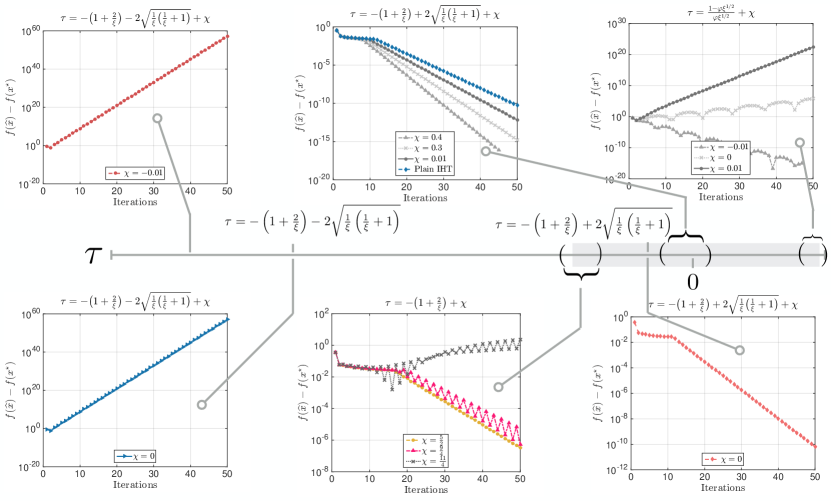
Figure 1. Behavior of accelerated IHT method, applied on a toy example for sparse linear regression. Consider 𝒜𝒜\mathcal{A} as the plain sparsity model, and let xsuperscript𝑥x^{\star} be a k𝑘k-sparse “signal” in 10superscript10\mathbb{R}^{10} for k=2𝑘2k=2, drawn from multivariate normal distribution. Also, x2=1subscriptnormsuperscript𝑥21\|x^{\star}\|_{2}=1. Let b=Φx𝑏Φsuperscript𝑥b=\Phi x^{\star}, with Φ6×10Φsuperscript610\Phi\in\mathbb{R}^{6\times 10} drawn entrywise i.i.d. from a normal distribution. Let \mathcal{I} be an index set of k𝑘k columns in ΦΦ\Phi; there are (nk)binomial𝑛𝑘{n\choose k} possible such subsets. By Definitions 1-2, we estimate α𝛼\alpha and β𝛽\beta as the λmin(ΦΦ)subscript𝜆superscriptsubscriptΦtopsubscriptΦ\lambda_{\min}(\Phi_{\mathcal{I}}^{\top}\Phi_{\mathcal{I}}) and λmax(ΦΦ)subscript𝜆superscriptsubscriptΦtopsubscriptΦ\lambda_{\max}(\Phi_{\mathcal{I}}^{\top}\Phi_{\mathcal{I}}), where ΦsubscriptΦ\Phi_{\mathcal{I}} is the submatrix of ΦΦ\Phi, indexed by \mathcal{I}. Here, α0.64𝛼0.64\alpha\approx 0.64 and β1.78𝛽1.78\beta\approx 1.78, which leads to ξ=1α/β0.94𝜉1𝛼𝛽0.94\xi=1-\nicefrac{{\alpha}}{{\beta}}\approx 0.94. We plot f(x^)f(x)𝑓^𝑥𝑓superscript𝑥f(\widehat{x})-f(x^{\star}) vs. iteration count, where f(x)=12bΦx22𝑓𝑥12superscriptsubscriptnorm𝑏Φ𝑥22f(x)=\tfrac{1}{2}\|b-\Phi x\|_{2}^{2}. Gray shaded area on τ𝜏\tau horizontal line corresponds to the range |τ|(1φξ1/2)/(φξ1/2)𝜏1𝜑superscript𝜉12𝜑superscript𝜉12|\tau|\leq(1-\varphi\xi^{1/2})/(\varphi\xi^{1/2}). (Left panel, top and bottom row). Accelerated IHT diverges for negative τ𝜏\tau, outside the τ𝜏\tau shaded area. (Middle panel, bottom row). “Rippling” behavior for τ𝜏\tau values close to the lower bound of converging τ𝜏\tau. (Middle panel, top row). Convergence behavior for accelerated IHT for various τ𝜏\tau values and its comparison to plain IHT (τ=0𝜏0\tau=0). (Right panel, top row). Similar “rippling” behavior as τ𝜏\tau approaches close to the upper bound of the shaded area; divergence is observed when τ𝜏\tau goes beyond the shaded area (observe that, for τ𝜏\tau values at the border of the shaded area, Algorithm 1 still diverges and this is due to the approximation of ξ𝜉\xi).

5. Related work

Optimization schemes over low-dimensional structured models have a long history; due to lack of space, we refer the reader to [23] for an overview of discrete and convex approaches. We note that there are both projected and proximal non-convex approaches that fit under our generic model, where no acceleration is assumed. E.g., see [4, 24, 15, 14]; our present work fills this gap. For non-convex proximal steps see [25] and references therein; again no acceleration is considered. Below, we focus on accelerated optimization variants, as well as Frank-Wolfe methods.

Related work on accelerated IHT variants. Accelerated IHT algorithms for sparse recovery were first introduced in [26, 19, 16]. In [26], the authors provide a double overrelaxation thresholding scheme [27] in order to accelerate their projected gradient descent variant for sparse linear regression; however, no theoretical guarantees are provided. In [19], Blumensath accelerates standard IHT methods for the same problem [9, 28] using the double overrelaxation technique in [26]. His result contains theoretical proof of linear convergence, under the assumption that the overrelaxation step is used only when the objective function decreases. However, this approach provides no guarantees that we might skip the acceleration term often, which leads back to the non-accelerated IHT version; see also [27] for a similar approach on EM algorithms. [29] describe a family of IHT variants, based on the conjugate gradient method [30], that includes under its umbrella methods like in [31, 32], with the option to perform acceleration steps; however, no theoretical justification for convergence is provided when acceleration motions are used. [16, 12] contain hard-thresholding variants, based on Nesterov’s ideas [17]; in [12], the authors provide convergence rate proofs for accelerated IHT when the objective is just least-squares; no generalization to convex f𝑓f is provided, neither a study on varied values of τ𝜏\tau. [33] includes a first attempt towards using adaptive τ𝜏\tau; his approach focuses on the least-squares objective, where a closed for solution for optimal τ𝜏\tau is found [16]. However, similar to [19], it is not guaranteed whether and how often the momentum is used, neither how to set up τ𝜏\tau in more generic objectives; see also Section D in the appendix. From a convex perspective, where the non-convex constraints are substituted by their convex relaxations (either in constrained or proximal setting), the work in [34] and [35] is relevant to the current work: based on two-step methods for linear systems [36], [34] extends these ideas to non-smooth (but convex) regularized linear systems, where f𝑓f is a least-squares term for image denoising purposes; see also [35]. Similar to [33, 19], [34] considers variants of accelerated convex gradient descent that guarantee monotonic decrease of function values per iteration.

Related work on acceleration techniques. Nesterov in [1] was the first to consider acceleration techniques in convex optimization settings; see also Chapter 2.2 in [17]. Such acceleration schemes have been widely used as black box in machine learning and signal processing [35, 34, 37, 38]. [6, 39] discuss restart heuristics, where momentum-related parameters are reset periodically after some iterations. [40] provides some adaptive restart strategies, along with analysis and intuition on why they work in practice for simple convex problems. Acceleration in non-convex settings have been very recently considered in continuous settings [41, 42, 43], where f𝑓f could be non-convex444The guarantees in these settings are restricted to finding a good stationary point.. However, none of these works, beyond [44], consider non-convex and possibly discontinuous constraints—for instance the subset of k𝑘k-sparse sets. In the case of [44], our work differs in that it explores better the low-dimensional constraint sets—however, we require f𝑓f to be convex. More relevant to this work is [45]: the authors consider non-convex proximal objective and apply ideas from [35] that lead to either monotone (skipping momentum steps) or nonmonotone function value decrease behavior; further, the theoretical guarantees are based on different tools than ours. We identify that such research questions could be directions for future work.

Related work on dynamical systems and numerical analysis. Multi-step schemes originate from explicit finite differences discretization of dynamical systems; e.g., the so-called Heavy-ball method [18] origins from the discretization of the friction dynamical system x¨(t)+γx˙(t)+f(x(t))=0¨𝑥𝑡𝛾˙𝑥𝑡𝑓𝑥𝑡0\ddot{x}(t)+\gamma\dot{x}(t)+\nabla f(x(t))=0, where γ>0𝛾0\gamma>0 plays the role of friction. Recent developments on this subject can be found in [46]; see also references therein. From a different perspective, Scieur et al. [47] use multi-step methods from numerical analysis to discretize the gradient flow equation. We believe that extending these ideas in non-convex domains (e.g., when non-convex constraints are included) is of potential interest for better understanding when and why momentum methods work in practical structured scenaria.

Related work on Frank-Wolfe variants: The Frank-Wolfe (FW) algorithm [5, 7] is an iterative projection-free convex scheme for constrained minimization. Frank-Wolfe often has cheap per iteration cost by solving a constrained linear program in each iteration. The classical analysis by [5] presents sublinear convergence for general functions. For strongly convex functions, FW admits linear convergence if the optimum does not lie on the boundary of the constraint set; in that case, the algorithm still has sublinear convergence rate. To address the boundary issue, [48] allows to move away from one of the already selected atoms, where linear convergence rate can be achieved [8]. Similarly, the pairwise variant introduced by [49] also has a linear convergent rate. This variant adjusts the weights of two of already selected atoms. [50] present a different perspective by showing linear convergence of classical FW over strongly convex sets and general functions. While several variants and sufficient conditions exist that admit linear convergence rates, the use of momentum for Frank-Wolfe, to the best of our knowledge is unexplored.
Refer to caption
Refer to caption
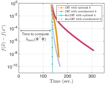
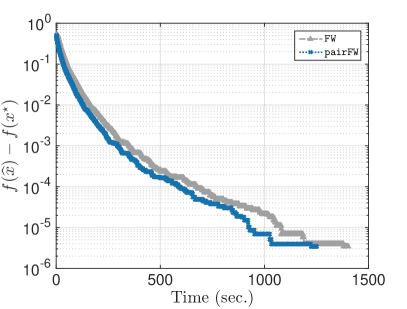
Figure 2. Time spent vs. function values gap f(x^)f(x)𝑓^𝑥𝑓superscript𝑥f(\widehat{x})-f(x^{\star}). AccIHT corresponds to Algorithm 1. Beware in left plot the time spent to approximate step size, via computing λmax(ΦΦ)subscript𝜆superscriptΦtopΦ\lambda_{\max}(\Phi^{\top}\Phi).
Refer to caption
Refer to caption
Refer to caption
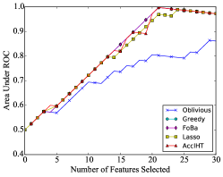
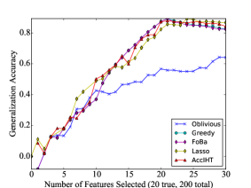
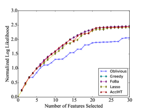
Figure 3. Empirical evaluation. Algorithm 1 achieves strong performance on true support recovery (left), generalization on test data (middle), and on training data fit (right)

6. Experiments

We conducted simulations for different problems to verify our predictions. In all experiments, we use constant τ=1/4𝜏14\tau=\nicefrac{{1}}{{4}} as a potential universal momentum parameter. Our experiments are proof of concept and demonstrate that accelerated projected gradient descent over non-convex structured sets can, not only offer high-quality recovery in practical settings, but offer much more scalable routines, compared to state-of-the-art. Here, we present only a subset of our experimental findings and we encourage readers to go over the experimental results in the Appendix E.

6.1. Sparse linear regression setting

For sparse linear regression, next we consider two simulated problems settings: (i)𝑖(i) with i.i.d. regressors, and (ii)𝑖𝑖(ii) with correlated regressors.

Sparse linear regression under the i.i.d. Gaussian setting: In this case, we consider a similar problem setting with [8], where xnsuperscript𝑥superscript𝑛x^{\star}\in\mathbb{R}^{n} is the unknown normalized k𝑘k-sparse vector, observed through the underdetermined set of linear equations: b=Φx𝑏Φsuperscript𝑥b=\Phi x^{\star}. Φm×nΦsuperscript𝑚𝑛\Phi\in\mathbb{R}^{m\times n} is drawn randomly from a normal distribution. We consider the standard least squares objective f(x)=12bΦx22𝑓𝑥12superscriptsubscriptnorm𝑏Φ𝑥22f(x)=\tfrac{1}{2}\|b-\Phi x\|_{2}^{2} and the plain sparsity model 𝒜𝒜\mathcal{A} where x0,𝒜x0subscriptnorm𝑥0𝒜subscriptnorm𝑥0\|x\|_{0,\mathcal{A}}\equiv\|x\|_{0}.

We compare Algorithm 1 (abbreviated as AccIHT in plots) with two FW variants (see [8] for FW and pairFW)555Phase transition results and comparisons to standard algorithms such as CoSaMP (restricted to squared loss) can be found in [16], and thus omitted. Further, according to [8], pairFW performs better than awayFW for this problem case, as well as the plain IHT algorithm. In this experiment, we use step sizes 1/β^1^𝛽1/\widehat{\beta} for Algorithm 1 and IHT, where β^=λmax(ΦΦ)^𝛽subscript𝜆superscriptΦtopΦ\widehat{\beta}=\lambda_{\max}(\Phi^{\top}\Phi), which is suboptimal compared to the step size theory dictates. For the FW variants, we follow the setup in [8] and set as the constraint set the λ𝜆\lambda-scaled 1subscript1\ell_{1}-norm ball, where λ=40𝜆40\lambda=40. In the FW code, we further “debias" the selected set of atoms per iteration, by performing fully corrective steps over putative solution (i.e., solve least-squares objective restricted over the active atom set) [16, 14]. We observed that such steps are necessary in our setting, in order FW to be competitive with Algorithm 1 and IHT. For IHT and Algorithm 1, we set input k𝑘k either exactly or use the 1subscript1\ell_{1}-norm phase transition plots [51], where the input parameter for sparsity k^^𝑘\widehat{k} is overshooted. See also Section B for more information. We compare the above algorithms w.r.t. function values decrease and running times.

Figure 2 depicts the summary of results we observed for the case n=2105𝑛2superscript105n=2\cdot 10^{5}, m=7500𝑚7500m=7500 and k=500𝑘500k=500. For IHT and accelerated IHT, we also consider the case where the input parameter for sparsity is set to k^=2441>k^𝑘2441𝑘\widehat{k}=2441>k. The graphs indicate that the accelerated hard thresholding technique can be much more efficient and scalable than the rest of the algorithms, while at the same time being at least as good in support/“signal" recovery performance. For instance, while Algorithm 1 is only 1.2×1.2\times faster than IHT, when k𝑘k is known exactly, Algorithm 1 is more resilient at overshooting k𝑘k: in that case, IHT could take >2×>2\times time to get to the same level of accuracy. At the same time, Algorithm 1 detects much faster the correct support, compared to plain IHT. Compared to FW methods (right plot), Algorithm 1 is at least 10×10\times faster than FW variants.

As stated before, we only focus on the optimization efficiency of the algorithms, not their statistical efficiency. That being said, we consider settings that are above the phase retrieval curve , and here we make no comparisons and claims regarding the number of samples required to complete the sparse linear regression task. We leave such work for an extended version of this work.

Sparse linear regression with correlated regressors: In this section, we test Algorithm 1 for support recovery, generalization and training loss performance in the sparse linear regression, under a different data generation setting. We generate the data as follows. We generate the feature matrix 800×200800200800\times 200 design matrix ΦΦ\Phi according to a first order auto-regressive process with correlation=0.4correlation0.4\texttt{correlation}=0.4. This ensures features are correlated with each other, which further makes feature selection a non-trivial task. We normalize the feature matrix so that each feature has 2subscript2\ell_{2}-norm equal to one. We generate an arbitrary weight vector xsuperscript𝑥x^{\star} with x0=20subscriptnormsuperscript𝑥020\|x^{\star}\|_{0}=20 and x2=1subscriptnormsuperscript𝑥21\|x^{\star}\|_{2}=1. The response vector b𝑏b is then computed as y=Φx+ε𝑦Φsuperscript𝑥𝜀y=\Phi x^{\star}+\varepsilon, where ε𝜀\varepsilon is guassian iid noise that is generated to ensure that the signal-to-noise ratio is 101010. Finally, the generated data is randomly split 505050-505050 into training and test sets.

We compare against Lasso [52], oblivious greedy selection (Oblivious [53]), forward greedy selection (Greedy [53]), and forward backward selection (FoBa [54]). The metrics we use to compare on are the generalization accuracy (R2superscript𝑅2R^{2} coefficient determination performance on test set), recovery of true support (AUC metric on predicted support vs. true support), and training data fit (log likelihood on the training set). The results are presented in Figure 3, and shows Algorithm 1 performs very competitively: it is almost always better or equal to other methods across different sparsity levels.

7. Overview and future directions

The use of hard-thresholding operations is widely known. In this work, we study acceleration techniques in simple hard-thresholding gradient procedures and characterize their performance; to the best of our knowledge, this is the first work to provide theoretical support for these type of algorithms. Our preliminary results show evidence that machine learning problems can be efficiently solved using our accelerated non-convex variant, which is at least competitive with state of the art and comes with convergence guarantees.

Our approach shows linear convergence; however, in theory, the acceleration achieved has dependence on the condition number of the problem not better than plain IHT. This leaves open the question on what types of conditions are sufficient to guarantee the better acceleration of momentum in such non-convex settings?

Apart from the future directions “scattered" in the main text, another possible direction lies at the intersection of dynamical systems and numerical analysis with optimization. Recent developments on this subject can be found in [46] and [47]. We believe that extending these ideas in non-convex domains is interesting to better understand when and why momentum methods work in practical structured scenaria.

References

  • [1] Y. Nesterov. A method of solving a convex programming problem with convergence rate O(1k2)1superscript𝑘2(\tfrac{1}{k^{2}}). In Soviet Mathematics Doklady, volume 27, pages 372–376, 1983.
  • [2] S. Negahban, B. Yu, M. Wainwright, and P. Ravikumar. A unified framework for high-dimensional analysis of m𝑚m-estimators with decomposable regularizers. In Advances in Neural Information Processing Systems, pages 1348–1356, 2009.
  • [3] V. Chandrasekaran, B. Recht, P. Parrilo, and A. Willsky. The convex geometry of linear inverse problems. Foundations of Computational mathematics, 12(6):805–849, 2012.
  • [4] S. Bahmani, B. Raj, and P. Boufounos. Greedy sparsity-constrained optimization. Journal of Machine Learning Research, 14(Mar):807–841, 2013.
  • [5] K. Clarkson. Coresets, sparse greedy approximation, and the Frank-Wolfe algorithm. ACM Transactions on Algorithms (TALG), 6(4):63, 2010.
  • [6] Y. Nesterov. Gradient methods for minimizing composite functions. Mathematical Programming, 140(1):125–161, 2013.
  • [7] M. Jaggi. Revisiting Frank-Wolfe: Projection-free sparse convex optimization. In ICML (1), pages 427–435, 2013.
  • [8] S. Lacoste-Julien and M. Jaggi. On the global linear convergence of Frank-Wolfe optimization variants. In Advances in Neural Information Processing Systems, pages 496–504, 2015.
  • [9] T. Blumensath and M. Davies. Iterative hard thresholding for compressed sensing. Applied and computational harmonic analysis, 27(3):265–274, 2009.
  • [10] P. Jain, R. Meka, and I. Dhillon. Guaranteed rank minimization via singular value projection. In Advances in Neural Information Processing Systems, pages 937–945, 2010.
  • [11] R. F. Barber and W. Ha. Gradient descent with nonconvex constraints: Local concavity determines convergence. arXiv preprint arXiv:1703.07755, 2017.
  • [12] A. Kyrillidis and V. Cevher. Matrix recipes for hard thresholding methods. Journal of mathematical imaging and vision, 48(2):235–265, 2014.
  • [13] F. Bach, R. Jenatton, J. Mairal, and G. Obozinski. Structured sparsity through convex optimization. Statistical Science, pages 450–468, 2012.
  • [14] P. Jain, N. Rao, and I. Dhillon. Structured sparse regression via greedy hard thresholding. In Advances in Neural Information Processing Systems, pages 1516–1524, 2016.
  • [15] P. Jain, A. Tewari, and P. Kar. On iterative hard thresholding methods for high-dimensional m𝑚m-estimation. In Advances in Neural Information Processing Systems, pages 685–693, 2014.
  • [16] A. Kyrillidis and V. Cevher. Recipes on hard thresholding methods. In Computational Advances in Multi-Sensor Adaptive Processing (CAMSAP), 2011 4th IEEE International Workshop on, pages 353–356. IEEE, 2011.
  • [17] Y. Nesterov. Introductory lectures on convex optimization: A basic course, volume 87. Springer Science & Business Media, 2013.
  • [18] B. Polyak. Some methods of speeding up the convergence of iteration methods. USSR Computational Mathematics and Mathematical Physics, 4(5):1–17, 1964.
  • [19] T. Blumensath. Accelerated iterative hard thresholding. Signal Processing, 92(3):752–756, 2012.
  • [20] A. Agarwal, S. Negahban, and M. Wainwright. Fast global convergence rates of gradient methods for high-dimensional statistical recovery. In Advances in Neural Information Processing Systems, pages 37–45, 2010.
  • [21] A. Beck and N. Hallak. On the minimization over sparse symmetric sets: projections, optimality conditions, and algorithms. Mathematics of Operations Research, 41(1):196–223, 2015.
  • [22] K. Williams. The n𝑛n-th power of a 2×2222\times 2 matrix. Mathematics Magazine, 65(5):336, 1992.
  • [23] A. Kyrillidis, L. Baldassarre, M. El Halabi, Q. Tran-Dinh, and V. Cevher. Structured sparsity: Discrete and convex approaches. In Compressed Sensing and its Applications, pages 341–387. Springer, 2015.
  • [24] X. Yuan, P. Li, and T. Zhang. Gradient hard thresholding pursuit for sparsity-constrained optimization. In Proceedings of the 31st International Conference on Machine Learning (ICML-14), pages 127–135, 2014.
  • [25] P. Gong, C. Zhang, Z. Lu, J. Huang, and J. Ye. A general iterative shrinkage and thresholding algorithm for non-convex regularized optimization problems. In ICML (2), pages 37–45, 2013.
  • [26] K. Qiu and A. Dogandzic. ECME thresholding methods for sparse signal reconstruction. arXiv preprint arXiv:1004.4880, 2010.
  • [27] R. Salakhutdinov and S. Roweis. Adaptive overrelaxed bound optimization methods. In Proceedings of the 20th International Conference on Machine Learning (ICML-03), pages 664–671, 2003.
  • [28] R. Garg and R. Khandekar. Gradient descent with sparsification: an iterative algorithm for sparse recovery with restricted isometry property. In Proceedings of the 26th Annual International Conference on Machine Learning, pages 337–344. ACM, 2009.
  • [29] J. Blanchard, J. Tanner, and K. Wei. CGIHT: Conjugate gradient iterative hard thresholding for compressed sensing and matrix completion. Information and Inference, 4(4):289–327, 2015.
  • [30] M. Hestenes and E. Stiefel. Methods of conjugate gradients for solving linear systems, volume 49. NBS, 1952.
  • [31] D. Needell and J. Tropp. CoSaMP: Iterative signal recovery from incomplete and inaccurate samples. Applied and Computational Harmonic Analysis, 26(3):301–321, 2009.
  • [32] S. Foucart. Hard thresholding pursuit: an algorithm for compressive sensing. SIAM Journal on Numerical Analysis, 49(6):2543–2563, 2011.
  • [33] K. Wei. Fast iterative hard thresholding for compressed sensing. IEEE Signal Processing Letters, 22(5):593–597, 2015.
  • [34] J. Bioucas-Dias and M. Figueiredo. A new TwIST: Two-step iterative shrinkage/thresholding algorithms for image restoration. IEEE Transactions on Image processing, 16(12):2992–3004, 2007.
  • [35] A. Beck and M. Teboulle. A fast iterative shrinkage-thresholding algorithm for linear inverse problems. SIAM journal on imaging sciences, 2(1):183–202, 2009.
  • [36] O. Axelsson. Iterative solution methods. Cambridge University press, 1996.
  • [37] M. Schmidt, N. Roux, and F. Bach. Convergence rates of inexact proximal-gradient methods for convex optimization. In Advances in neural information processing systems, pages 1458–1466, 2011.
  • [38] S. Shalev-Shwartz and T. Zhang. Accelerated proximal stochastic dual coordinate ascent for regularized loss minimization. In ICML, pages 64–72, 2014.
  • [39] S. Becker, E. Candès, and M. Grant. Templates for convex cone problems with applications to sparse signal recovery. Mathematical programming computation, 3(3):165–218, 2011.
  • [40] B. O’Donoghue and E. Candes. Adaptive restart for accelerated gradient schemes. Foundations of computational mathematics, 15(3):715–732, 2015.
  • [41] S. Ghadimi and G. Lan. Accelerated gradient methods for nonconvex nonlinear and stochastic programming. Mathematical Programming, 156(1-2):59–99, 2016.
  • [42] Y. Carmon, J. Duchi, O. Hinder, and A. Sidford. Accelerated methods for non-convex optimization. arXiv preprint arXiv:1611.00756, 2016.
  • [43] N. Agarwal, Z. Allen-Zhu, B. Bullins, E. Hazan, and T. Ma. Finding approximate local minima for nonconvex optimization in linear time. arXiv preprint arXiv:1611.01146, 2016.
  • [44] C. Paquette, H. Lin, D. Drusvyatskiy, J. Mairal, and Z. Harchaoui. Catalyst acceleration for gradient-based non-convex optimization. arXiv preprint arXiv:1703.10993, 2017.
  • [45] H. Li and Z. Lin. Accelerated proximal gradient methods for nonconvex programming. In Advances in neural information processing systems, pages 379–387, 2015.
  • [46] A. Wilson, B. Recht, and M. Jordan. A lyapunov analysis of momentum methods in optimization. arXiv preprint arXiv:1611.02635, 2016.
  • [47] D. Scieur, V. Roulet, F. Bach, and A. d’Aspremont. Integration methods and accelerated optimization algorithms. arXiv preprint arXiv:1702.06751, 2017.
  • [48] P. Wolfe. Convergence theory in nonlinear programming. Integer and nonlinear programming, pages 1–36, 1970.
  • [49] B. Mitchell, V. Demyanov, and V. Malozemov. Finding the point of a polyhedron closest to the origin. SIAM Journal on Control, 12(1):19–26, 1974.
  • [50] D. Garber and E. Hazan. Faster rates for the Frank-Wolfe method over strongly-convex sets. In ICML, pages 541–549, 2015.
  • [51] D. Donoho and J. Tanner. Neighborliness of randomly projected simplices in high dimensions. Proceedings of the National Academy of Sciences of the United States of America, 102(27):9452–9457, 2005.
  • [52] F. Pedregosa, G. Varoquaux, A. Gramfort, V. Michel, B. Thirion, O. Grisel, M. Blondel, P. Prettenhofer, R. Weiss, V. Dubourg, J. Vanderplas, A. Passos, D. Cournapeau, M. Brucher, M. Perrot, and E. Duchesnay. Scikit-learn: Machine learning in Python. Journal of Machine Learning Research, 12:2825–2830, 2011.
  • [53] A. Das and D. Kempe. Submodular meets spectral: Greedy algorithms for subset selection, sparse approximation and dictionary selection. In Proceedings of the 28th International Conference on Machine Learning (ICML-11), pages 1057–1064, 2011.
  • [54] T. Zhang. Adaptive forward-backward greedy algorithm for sparse learning with linear models. In Advances in Neural Information Processing Systems, pages 1921–1928, 2009.
  • [55] S. Chen, D. Donoho, and M. Saunders. Atomic decomposition by basis pursuit. SIAM review, 43(1):129–159, 2001.
  • [56] B. Recht, M. Fazel, and P. Parrilo. Guaranteed minimum-rank solutions of linear matrix equations via nuclear norm minimization. SIAM review, 52(3):471–501, 2010.
  • [57] A. Tillmann and M. Pfetsch. The computational complexity of the restricted isometry property, the nullspace property, and related concepts in compressed sensing. IEEE Transactions on Information Theory, 60(2):1248–1259, 2014.
  • [58] T. Blumensath. Sampling and reconstructing signals from a union of linear subspaces. IEEE Transactions on Information Theory, 57(7):4660–4671, 2011.
  • [59] P. Shah and V. Chandrasekaran. Iterative projections for signal identification on manifolds: Global recovery guarantees. In Communication, Control, and Computing (Allerton), 2011 49th Annual Allerton Conference on, pages 760–767. IEEE, 2011.
  • [60] A. Kyrillidis and V. Cevher. Combinatorial selection and least absolute shrinkage via the CLASH algorithm. In Information Theory Proceedings (ISIT), 2012 IEEE International Symposium on, pages 2216–2220. IEEE, 2012.
  • [61] C. Hegde, P. Indyk, and L. Schmidt. Approximation algorithms for model-based compressive sensing. IEEE Transactions on Information Theory, 61(9):5129–5147, 2015.
  • [62] L. Jacob, G. Obozinski, and J.-P. Vert. Group lasso with overlap and graph lasso. In Proceedings of the 26th annual international conference on machine learning, pages 433–440. ACM, 2009.
  • [63] S. Negahban and M. Wainwright. Restricted strong convexity and weighted matrix completion: Optimal bounds with noise. Journal of Machine Learning Research, 13(May):1665–1697, 2012.
  • [64] S. Bhojanapalli, A. Kyrillidis, and S. Sanghavi. Dropping convexity for faster semi-definite optimization. In Conference on Learning Theory, pages 530–582, 2016.
  • [65] D. Park, A. Kyrillidis, C. Caramanis, and S. Sanghavi. Finding low-rank solutions to matrix problems, efficiently and provably. arXiv preprint arXiv:1606.03168, 2016.

Appendix A Proof of Lemma 1

We start by observing that: xi+1u¯i22xu¯i22superscriptsubscriptnormsubscript𝑥𝑖1subscript¯𝑢𝑖22superscriptsubscriptnormsuperscript𝑥subscript¯𝑢𝑖22\|x_{i+1}-\bar{u}_{i}\|_{2}^{2}\leq\|x^{\star}-\bar{u}_{i}\|_{2}^{2}, due to the exactness of the hard thresholding operation. Note that this holds for most 𝒜𝒜\mathcal{A} of interest666For example, in the case of matrices and low-rankness, this operation holds due to the Eckart-Young-Mirsky-Steward theorem, and the inner products of vectors naturally extend to the inner products over matrices. but, again for simplicity, we will focus on the sparsity model here. By adding and subtracting xsuperscript𝑥x^{\star} and expanding the squares, we get:

xi+1x+xu¯i22superscriptsubscriptnormsubscript𝑥𝑖1superscript𝑥superscript𝑥subscript¯𝑢𝑖22\displaystyle\|x_{i+1}-x^{\star}+x^{\star}-\bar{u}_{i}\|_{2}^{2} xu¯i22absentsuperscriptsubscriptnormsuperscript𝑥subscript¯𝑢𝑖22absent\displaystyle\leq\|x^{\star}-\bar{u}_{i}\|_{2}^{2}\Rightarrow
xi+1x22+xu¯i22+2xi+1x,xu¯isuperscriptsubscriptnormsubscript𝑥𝑖1superscript𝑥22superscriptsubscriptnormsuperscript𝑥subscript¯𝑢𝑖222subscript𝑥𝑖1superscript𝑥superscript𝑥subscript¯𝑢𝑖\displaystyle\|x_{i+1}-x^{\star}\|_{2}^{2}+\|x^{\star}-\bar{u}_{i}\|_{2}^{2}+2\left\langle x_{i+1}-x^{\star},~{}x^{\star}-\bar{u}_{i}\right\rangle xu¯i22absentsuperscriptsubscriptnormsuperscript𝑥subscript¯𝑢𝑖22absent\displaystyle\leq\|x^{\star}-\bar{u}_{i}\|_{2}^{2}\Rightarrow
xi+1x22superscriptsubscriptnormsubscript𝑥𝑖1superscript𝑥22\displaystyle\|x_{i+1}-x^{\star}\|_{2}^{2} 2xi+1x,u¯ixabsent2subscript𝑥𝑖1superscript𝑥subscript¯𝑢𝑖superscript𝑥\displaystyle\leq 2\left\langle x_{i+1}-x^{\star},~{}\bar{u}_{i}-x^{\star}\right\rangle

We also know that:

u¯isubscript¯𝑢𝑖\displaystyle\bar{u}_{i} =uiμi𝒯if(ui)absentsubscript𝑢𝑖subscript𝜇𝑖subscriptsubscript𝒯𝑖𝑓subscript𝑢𝑖\displaystyle=u_{i}-\mu_{i}\nabla_{\mathcal{T}_{i}}f(u_{i})
=ui+μiΦ𝒯i(bΦ𝒯iui)absentsubscript𝑢𝑖subscript𝜇𝑖superscriptsubscriptΦsubscript𝒯𝑖top𝑏subscriptΦsubscript𝒯𝑖subscript𝑢𝑖\displaystyle=u_{i}+\mu_{i}\Phi_{\mathcal{T}_{i}}^{\top}(b-\Phi_{\mathcal{T}_{i}}u_{i})
=ui+μiΦ𝒯i(Φ𝒯ix+εΦ𝒯iui)absentsubscript𝑢𝑖subscript𝜇𝑖superscriptsubscriptΦsubscript𝒯𝑖topsubscriptΦsubscript𝒯𝑖superscript𝑥𝜀subscriptΦsubscript𝒯𝑖subscript𝑢𝑖\displaystyle=u_{i}+\mu_{i}\Phi_{\mathcal{T}_{i}}^{\top}(\Phi_{\mathcal{T}_{i}}x^{\star}+\varepsilon-\Phi_{\mathcal{T}_{i}}u_{i})
=ui+μiΦ𝒯iΦ𝒯i(xui)+μiΦ𝒯iεabsentsubscript𝑢𝑖subscript𝜇𝑖superscriptsubscriptΦsubscript𝒯𝑖topsubscriptΦsubscript𝒯𝑖superscript𝑥subscript𝑢𝑖subscript𝜇𝑖superscriptsubscriptΦsubscript𝒯𝑖top𝜀\displaystyle=u_{i}+\mu_{i}\Phi_{\mathcal{T}_{i}}^{\top}\Phi_{\mathcal{T}_{i}}\left(x^{\star}-u_{i}\right)+\mu_{i}\Phi_{\mathcal{T}_{i}}^{\top}\varepsilon

Going back to the original inequality, we obtain:

xi+1x22superscriptsubscriptnormsubscript𝑥𝑖1superscript𝑥22\displaystyle\|x_{i+1}-x^{\star}\|_{2}^{2} 2xi+1x,ui+μiΦ𝒯iΦ𝒯i(xui)+μiΦ𝒯iεxabsent2subscript𝑥𝑖1superscript𝑥subscript𝑢𝑖subscript𝜇𝑖superscriptsubscriptΦsubscript𝒯𝑖topsubscriptΦsubscript𝒯𝑖superscript𝑥subscript𝑢𝑖subscript𝜇𝑖superscriptsubscriptΦsubscript𝒯𝑖top𝜀superscript𝑥\displaystyle\leq 2\left\langle x_{i+1}-x^{\star},~{}u_{i}+\mu_{i}\Phi_{\mathcal{T}_{i}}^{\top}\Phi_{\mathcal{T}_{i}}\left(x^{\star}-u_{i}\right)+\mu_{i}\Phi_{\mathcal{T}_{i}}^{\top}\varepsilon-x^{\star}\right\rangle
=2xi+1x,(IμiΦ𝒯iΦ𝒯i)(uix)+2xi+1x,μiΦ𝒯iεabsent2subscript𝑥𝑖1superscript𝑥𝐼subscript𝜇𝑖superscriptsubscriptΦsubscript𝒯𝑖topsubscriptΦsubscript𝒯𝑖subscript𝑢𝑖superscript𝑥2subscript𝑥𝑖1superscript𝑥subscript𝜇𝑖superscriptsubscriptΦsubscript𝒯𝑖top𝜀\displaystyle=2\left\langle x_{i+1}-x^{\star},~{}\left(I-\mu_{i}\Phi_{\mathcal{T}_{i}}^{\top}\Phi_{\mathcal{T}_{i}}\right)\left(u_{i}-x^{\star}\right)\right\rangle+2\left\langle x_{i+1}-x^{\star},~{}\mu_{i}\Phi_{\mathcal{T}_{i}}^{\top}\varepsilon\right\rangle
2xi+1x2(IμiΦ𝒯iΦ𝒯i)(uix)2+2μiΦ𝒯i(xi+1x)2ε2absent2subscriptnormsubscript𝑥𝑖1superscript𝑥2subscriptnorm𝐼subscript𝜇𝑖superscriptsubscriptΦsubscript𝒯𝑖topsubscriptΦsubscript𝒯𝑖subscript𝑢𝑖superscript𝑥22subscript𝜇𝑖subscriptnormsubscriptΦsubscript𝒯𝑖subscript𝑥𝑖1superscript𝑥2subscriptnorm𝜀2\displaystyle\leq 2\left\|x_{i+1}-x^{\star}\right\|_{2}\cdot\left\|\left(I-\mu_{i}\Phi_{\mathcal{T}_{i}}^{\top}\Phi_{\mathcal{T}_{i}}\right)\left(u_{i}-x^{\star}\right)\right\|_{2}+2\mu_{i}\left\|\Phi_{\mathcal{T}_{i}}\left(x_{i+1}-x^{\star}\right)\right\|_{2}\cdot\left\|\varepsilon\right\|_{2}
2xi+1x2IμiΦ𝒯iΦ𝒯i2uix2+2μiΦ𝒯i(xi+1x)2ε2absent2subscriptnormsubscript𝑥𝑖1superscript𝑥2subscriptnorm𝐼subscript𝜇𝑖superscriptsubscriptΦsubscript𝒯𝑖topsubscriptΦsubscript𝒯𝑖2subscriptnormsubscript𝑢𝑖superscript𝑥22subscript𝜇𝑖subscriptnormsubscriptΦsubscript𝒯𝑖subscript𝑥𝑖1superscript𝑥2subscriptnorm𝜀2\displaystyle\leq 2\left\|x_{i+1}-x^{\star}\right\|_{2}\cdot\left\|I-\mu_{i}\Phi_{\mathcal{T}_{i}}^{\top}\Phi_{\mathcal{T}_{i}}\right\|_{2}\cdot\left\|u_{i}-x^{\star}\right\|_{2}+2\mu_{i}\left\|\Phi_{\mathcal{T}_{i}}\left(x_{i+1}-x^{\star}\right)\right\|_{2}\cdot\left\|\varepsilon\right\|_{2}

Using the properties of generalized restricted isometry property, we observe that: Φ𝒯i(xi+1x)2β2kxi+1x2subscriptnormsubscriptΦsubscript𝒯𝑖subscript𝑥𝑖1superscript𝑥2subscript𝛽2𝑘subscriptnormsubscript𝑥𝑖1superscript𝑥2\left\|\Phi_{\mathcal{T}_{i}}\left(x_{i+1}-x^{\star}\right)\right\|_{2}\leq\sqrt{\beta_{2k}}\|x_{i+1}-x^{\star}\|_{2}, and:

IμiΦ𝒯iΦ𝒯i2β3kα3kα3k+β3ksubscriptnorm𝐼subscript𝜇𝑖superscriptsubscriptΦsubscript𝒯𝑖topsubscriptΦsubscript𝒯𝑖2subscript𝛽3𝑘subscript𝛼3𝑘subscript𝛼3𝑘subscript𝛽3𝑘\displaystyle\left\|I-\mu_{i}\Phi_{\mathcal{T}_{i}}^{\top}\Phi_{\mathcal{T}_{i}}\right\|_{2}\leq\frac{\beta_{3k}-\alpha_{3k}}{\alpha_{3k}+\beta_{3k}}

In the last inequality we use the generalized RIP:

αrkx22Φx22βrkx22,subscript𝛼𝑟𝑘superscriptsubscriptnorm𝑥22superscriptsubscriptnormΦ𝑥22subscript𝛽𝑟𝑘superscriptsubscriptnorm𝑥22\displaystyle\alpha_{rk}\|x\|_{2}^{2}\leq\|\Phi x\|_{2}^{2}\leq\beta_{rk}\|x\|_{2}^{2},

and the fact that we can minimize with respect to μisubscript𝜇𝑖\mu_{i} to get:

minμiIμiΦ𝒯iΦ𝒯i2minμimax{μiβ3k1,1μiα3k}=β3kα3kα3k+β3ksubscriptsubscript𝜇𝑖subscriptnorm𝐼subscript𝜇𝑖superscriptsubscriptΦsubscript𝒯𝑖topsubscriptΦsubscript𝒯𝑖2subscriptsubscript𝜇𝑖subscript𝜇𝑖subscript𝛽3𝑘11subscript𝜇𝑖subscript𝛼3𝑘subscript𝛽3𝑘subscript𝛼3𝑘subscript𝛼3𝑘subscript𝛽3𝑘\displaystyle\min_{\mu_{i}}\left\|I-\mu_{i}\Phi_{\mathcal{T}_{i}}^{\top}\Phi_{\mathcal{T}_{i}}\right\|_{2}\leq\min_{\mu_{i}}\max\{\mu_{i}\beta_{3k}-1,~{}1-\mu_{i}\alpha_{3k}\}=\frac{\beta_{3k}-\alpha_{3k}}{\alpha_{3k}+\beta_{3k}}

for μi=2α3k+β3ksubscript𝜇𝑖2subscript𝛼3𝑘subscript𝛽3𝑘\mu_{i}=\frac{2}{\alpha_{3k}+\beta_{3k}}.

The above lead to:

xi+1x22superscriptsubscriptnormsubscript𝑥𝑖1superscript𝑥22\displaystyle\|x_{i+1}-x^{\star}\|_{2}^{2} 2xi+1x2β3kα3kα3k+β3kuix2+2β2kα3k+β3kxi+1x2ε2absent2subscriptnormsubscript𝑥𝑖1superscript𝑥2subscript𝛽3𝑘subscript𝛼3𝑘subscript𝛼3𝑘subscript𝛽3𝑘subscriptnormsubscript𝑢𝑖superscript𝑥22subscript𝛽2𝑘subscript𝛼3𝑘subscript𝛽3𝑘subscriptnormsubscript𝑥𝑖1superscript𝑥2subscriptnorm𝜀2absent\displaystyle\leq 2\left\|x_{i+1}-x^{\star}\right\|_{2}\tfrac{\beta_{3k}-\alpha_{3k}}{\alpha_{3k}+\beta_{3k}}\cdot\left\|u_{i}-x^{\star}\right\|_{2}+\tfrac{2\sqrt{\beta_{2k}}}{\alpha_{3k}+\beta_{3k}}\|x_{i+1}-x^{\star}\|_{2}\cdot\left\|\varepsilon\right\|_{2}\Rightarrow
xi+1x2subscriptnormsubscript𝑥𝑖1superscript𝑥2\displaystyle\|x_{i+1}-x^{\star}\|_{2} 2(β3kα3k)α3k+β3kuix2+2β2kα3k+β3kε2absent2subscript𝛽3𝑘subscript𝛼3𝑘subscript𝛼3𝑘subscript𝛽3𝑘subscriptnormsubscript𝑢𝑖superscript𝑥22subscript𝛽2𝑘subscript𝛼3𝑘subscript𝛽3𝑘subscriptnorm𝜀2\displaystyle\leq\tfrac{2(\beta_{3k}-\alpha_{3k})}{\alpha_{3k}+\beta_{3k}}\cdot\left\|u_{i}-x^{\star}\right\|_{2}+\tfrac{2\sqrt{\beta_{2k}}}{\alpha_{3k}+\beta_{3k}}\left\|\varepsilon\right\|_{2}

Defining κ=β3kα3k𝜅subscript𝛽3𝑘subscript𝛼3𝑘\kappa=\frac{\beta_{3k}}{\alpha_{3k}} as the condition number, we get:

xi+1x2subscriptnormsubscript𝑥𝑖1superscript𝑥2\displaystyle\|x_{i+1}-x^{\star}\|_{2} 2(κ1)κ+1uix2+2β2kα3k+β3kε2absent2𝜅1𝜅1subscriptnormsubscript𝑢𝑖superscript𝑥22subscript𝛽2𝑘subscript𝛼3𝑘subscript𝛽3𝑘subscriptnorm𝜀2\displaystyle\leq\tfrac{2(\kappa-1)}{\kappa+1}\cdot\left\|u_{i}-x^{\star}\right\|_{2}+\tfrac{2\sqrt{\beta_{2k}}}{\alpha_{3k}+\beta_{3k}}\left\|\varepsilon\right\|_{2}

Focusing on the norm term on RHS, we observe:

uix2subscriptnormsubscript𝑢𝑖superscript𝑥2\displaystyle\|u_{i}-x^{\star}\|_{2} =xi+τi(xixi1)x2=xi+τi(xixi1)(1τi+τi)x2absentsubscriptnormsubscript𝑥𝑖subscript𝜏𝑖subscript𝑥𝑖subscript𝑥𝑖1superscript𝑥2subscriptnormsubscript𝑥𝑖subscript𝜏𝑖subscript𝑥𝑖subscript𝑥𝑖11subscript𝜏𝑖subscript𝜏𝑖superscript𝑥2\displaystyle=\|x_{i}+\tau_{i}\left(x_{i}-x_{i-1}\right)-x^{\star}\|_{2}=\|x_{i}+\tau_{i}\left(x_{i}-x_{i-1}\right)-(1-\tau_{i}+\tau_{i})x^{\star}\|_{2}
=(1+τi)(xix)+τi(xxi1)2absentsubscriptnorm1subscript𝜏𝑖subscript𝑥𝑖superscript𝑥subscript𝜏𝑖superscript𝑥subscript𝑥𝑖12\displaystyle=\|(1+\tau_{i})(x_{i}-x^{\star})+\tau_{i}(x^{\star}-x_{i-1})\|_{2}
|1+τ|xix2+|τ|xi1x2absent1𝜏subscriptnormsubscript𝑥𝑖superscript𝑥2𝜏subscriptnormsubscript𝑥𝑖1superscript𝑥2\displaystyle\leq|1+\tau|\cdot\|x_{i}-x^{\star}\|_{2}+|\tau|\cdot\|x_{i-1}-x^{\star}\|_{2}

where in the last inequality we used the triangle inequality and the fact that τi=τsubscript𝜏𝑖𝜏\tau_{i}=\tau, for all i𝑖i. Substituting this in our main inequality, we get:

xi+1x2subscriptnormsubscript𝑥𝑖1superscript𝑥2\displaystyle\|x_{i+1}-x^{\star}\|_{2} 2(κ1)κ+1(|1+τ|xix2+|τ|xi1x2)+2β2kα3k+β3kε2absent2𝜅1𝜅11𝜏subscriptnormsubscript𝑥𝑖superscript𝑥2𝜏subscriptnormsubscript𝑥𝑖1superscript𝑥22subscript𝛽2𝑘subscript𝛼3𝑘subscript𝛽3𝑘subscriptnorm𝜀2\displaystyle\leq\tfrac{2(\kappa-1)}{\kappa+1}\cdot\left(|1+\tau|\cdot\|x_{i}-x^{\star}\|_{2}+|\tau|\cdot\|x_{i-1}-x^{\star}\|_{2}\right)+\tfrac{2\sqrt{\beta_{2k}}}{\alpha_{3k}+\beta_{3k}}\left\|\varepsilon\right\|_{2}
=2(κ1)κ+1|1+τ|xix2+2(κ1)κ+1|τ|xi1x2+2β2kα3k+β3kε2absent2𝜅1𝜅11𝜏subscriptnormsubscript𝑥𝑖superscript𝑥22𝜅1𝜅1𝜏subscriptnormsubscript𝑥𝑖1superscript𝑥22subscript𝛽2𝑘subscript𝛼3𝑘subscript𝛽3𝑘subscriptnorm𝜀2\displaystyle=\tfrac{2(\kappa-1)}{\kappa+1}\cdot|1+\tau|\cdot\|x_{i}-x^{\star}\|_{2}+\tfrac{2(\kappa-1)}{\kappa+1}\cdot|\tau|\cdot\|x_{i-1}-x^{\star}\|_{2}+\tfrac{2\sqrt{\beta_{2k}}}{\alpha_{3k}+\beta_{3k}}\left\|\varepsilon\right\|_{2}

Define z(i)=xix2𝑧𝑖subscriptnormsubscript𝑥𝑖superscript𝑥2z(i)=\|x_{i}-x^{\star}\|_{2}; this leads to the following second-order linear system:

z(i+1)2(κ1)κ+1|1+τ|z(i)+2(κ1)κ+1|τ|z(i1)+2β2kα3k+β3kε2.𝑧𝑖12𝜅1𝜅11𝜏𝑧𝑖2𝜅1𝜅1𝜏𝑧𝑖12subscript𝛽2𝑘subscript𝛼3𝑘subscript𝛽3𝑘subscriptnorm𝜀2\displaystyle z(i+1)\leq\tfrac{2(\kappa-1)}{\kappa+1}\cdot|1+\tau|\cdot z(i)+\tfrac{2(\kappa-1)}{\kappa+1}\cdot|\tau|\cdot z(i-1)+\tfrac{2\sqrt{\beta_{2k}}}{\alpha_{3k}+\beta_{3k}}\left\|\varepsilon\right\|_{2}.

We can convert this second-order linear system into a two-dimensional first-order system, where the variables of the linear system are multi-dimensional. To do this, we define a new state variable w(i)𝑤𝑖w(i):

w(i):=z(i+1)assign𝑤𝑖𝑧𝑖1\displaystyle w(i):=z(i+1)

and thus w(i+1)=z(i+2)𝑤𝑖1𝑧𝑖2w(i+1)=z(i+2). Using w(i)𝑤𝑖w(i), we define the following 2-dimensional, first-order system:

{w(i)2(κ1)κ+1|1+τ|w(i1)2(κ1)κ+1|τ|z(i1)2β2kα3k+β3kε20,z(i)w(i1).cases𝑤𝑖2𝜅1𝜅11𝜏𝑤𝑖12𝜅1𝜅1𝜏𝑧𝑖12subscript𝛽2𝑘subscript𝛼3𝑘subscript𝛽3𝑘subscriptnorm𝜀20missing-subexpression𝑧𝑖𝑤𝑖1missing-subexpression\displaystyle\left\{\begin{array}[]{ll}w(i)-\tfrac{2(\kappa-1)}{\kappa+1}\cdot|1+\tau|\cdot w(i-1)-\tfrac{2(\kappa-1)}{\kappa+1}\cdot|\tau|\cdot z(i-1)-\tfrac{2\sqrt{\beta_{2k}}}{\alpha_{3k}+\beta_{3k}}\left\|\varepsilon\right\|_{2}\leq 0,\\ z(i)\leq w(i-1).\end{array}\right.

This further characterizes the evolution of two state variables, {w(i),z(i)}𝑤𝑖𝑧𝑖\{w(i),z(i)\}:

[w(i)z(i)]matrix𝑤𝑖𝑧𝑖\displaystyle\begin{bmatrix}w(i)\\ z(i)\end{bmatrix} [2(κ1)κ+1|1+τ|2(κ1)κ+1|τ|10][w(i1)z(i1)]+[10]2β2kα3k+β3kε2absentmatrix2𝜅1𝜅11𝜏2𝜅1𝜅1𝜏10matrix𝑤𝑖1𝑧𝑖1matrix102subscript𝛽2𝑘subscript𝛼3𝑘subscript𝛽3𝑘subscriptnorm𝜀2absent\displaystyle\leq\begin{bmatrix}\tfrac{2(\kappa-1)}{\kappa+1}\cdot|1+\tau|&\tfrac{2(\kappa-1)}{\kappa+1}\cdot|\tau|\\ 1&0\end{bmatrix}\cdot\begin{bmatrix}w(i-1)\\ z(i-1)\end{bmatrix}+\begin{bmatrix}1\\ 0\end{bmatrix}\tfrac{2\sqrt{\beta_{2k}}}{\alpha_{3k}+\beta_{3k}}\left\|\varepsilon\right\|_{2}\Rightarrow
[xi+1x2xix2]matrixsubscriptnormsubscript𝑥𝑖1superscript𝑥2subscriptnormsubscript𝑥𝑖superscript𝑥2\displaystyle\begin{bmatrix}\|x_{i+1}-x^{\star}\|_{2}\\ \|x_{i}-x^{\star}\|_{2}\end{bmatrix} [2(κ1)κ+1|1+τ|2(κ1)κ+1|τ|10][xix2xi1x2]+[10]2β2kα3k+β3kε2,absentmatrix2𝜅1𝜅11𝜏2𝜅1𝜅1𝜏10matrixsubscriptnormsubscript𝑥𝑖superscript𝑥2subscriptnormsubscript𝑥𝑖1superscript𝑥2matrix102subscript𝛽2𝑘subscript𝛼3𝑘subscript𝛽3𝑘subscriptnorm𝜀2\displaystyle\leq\begin{bmatrix}\tfrac{2(\kappa-1)}{\kappa+1}\cdot|1+\tau|&\tfrac{2(\kappa-1)}{\kappa+1}\cdot|\tau|\\ 1&0\end{bmatrix}\cdot\begin{bmatrix}\|x_{i}-x^{\star}\|_{2}\\ \|x_{i-1}-x^{\star}\|_{2}\end{bmatrix}+\begin{bmatrix}1\\ 0\end{bmatrix}\tfrac{2\sqrt{\beta_{2k}}}{\alpha_{3k}+\beta_{3k}}\left\|\varepsilon\right\|_{2},

where in the last inequality we use the definitions z(i)=xix2𝑧𝑖subscriptnormsubscript𝑥𝑖superscript𝑥2z(i)=\|x_{i}-x^{\star}\|_{2} and w(i)=z(i+1)𝑤𝑖𝑧𝑖1w(i)=z(i+1). Observe that the contraction matrix has non-negative values. This completes the proof.

Appendix B Implementation details

So far, we have showed the theoretical performance of our algorithm, where several hyper-parameters are assumed known. Here, we discuss a series of practical matters that arise in the implementation of our algorithm.

B.1. Setting structure hyper-parameter k𝑘k

Given structure 𝒜𝒜\mathcal{A}, one needs to set the “succinctness" level k𝑘k, as input to Algorithm 1. Before we describe practical solutions on how to set up this value, we first note that selecting k𝑘k is often intuitively easier than setting the regularization parameter in convexified versions of (4). For instance, in vector sparsity settings for linear systems, where the Lasso criterion is used: argminxn{12bΦx22+λx1}subscriptargmin𝑥superscript𝑛12superscriptsubscriptnorm𝑏Φ𝑥22𝜆subscriptnorm𝑥1\operatorname*{arg\,min}_{x\in\mathbb{R}^{n}}\left\{\tfrac{1}{2}\|b-\Phi x\|_{2}^{2}+\lambda\cdot\|x\|_{1}\right\}, selecting λ>0𝜆0\lambda>0 is a non-trivial task: arbitrary values of λ𝜆\lambda lead to different k𝑘k, and it is not obvious what is the “sweet range" of λ𝜆\lambda values for a particular sparsity level. From that perspective, using k𝑘k leads to more interpretable results.

However, even in the strict discrete case, selecting k𝑘k could be considered art for many cases. Here, we propose two ways for such selection: (i)𝑖(i) via cross-validation, and (ii)𝑖𝑖(ii) by using phase transition plots. Regarding cross-validation, this is a well-known technique and we will skip the details; we note that we used cross-validation, as in [14], to select the group sparsity parameters for the tumor classification problem in Subsection E.1.

A different way to select k𝑘k comes from the recovery limits of the optimization scheme at hand: For simplicity, consider the least-squares objective with sparsity constraints. [51] describes mathematically the phase transition behavior of the basis pursuit algorithm [55] for that problem; see Figure 1 in [51]. Moving along the phase transition line, triplets of (m,n,k)𝑚𝑛𝑘(m,n,k) can be extracted; for fixed m𝑚m and n𝑛n, this results into a unique value for k𝑘k. We used this “overshooted" value in Algorithm 1 at our experiments for sparse linear regression; see Figure 2 in Subsection 6.1. Our results show that, even using this procedure as a heuristic, it results into an automatic way of setting k𝑘k, that leads to the correct solution. Similar phase transition plots can be extracted, even experimentally, for other structures 𝒜𝒜\mathcal{A}; see e.g. [56] for the case of low rankness.

B.2. Selecting τ𝜏\tau and step size in practice

The analysis in Section 4 suggests using τ𝜏\tau within the range: |τ|(1φξ1/2)φξ1/2𝜏1𝜑superscript𝜉12𝜑superscript𝜉12|\tau|\leq\tfrac{(1-\varphi\cdot\xi^{1/2})}{\varphi\cdot\xi^{1/2}}. In order to compute the end points of this range, we require a good approximation of ξ:=1α/βassign𝜉1𝛼𝛽\xi:=1-\nicefrac{{\alpha}}{{\beta}}, where α𝛼\alpha and β𝛽\beta are the restricted strong convexity and smoothness parameters of f𝑓f, respectively.

In general, computing α𝛼\alpha and β𝛽\beta in practice is an NP-hard task777To see this, in the sparse linear regression setting, there is a connection between α,β𝛼𝛽\alpha,\beta and the so-called restricted isometry constants [57]. It is well known that the latter is NP-hard to compute. A practical rule is to use a constant momentum term, like τ=1/4𝜏14\tau=\nicefrac{{1}}{{4}}: we observed that this value worked well in our experiments.888We did not perform binary search for this selection—we conjecture that better τ𝜏\tau values in our results could result into even more significant gains w.r.t. convergence rates.

In some cases, one can approximate α𝛼\alpha and β𝛽\beta with the smallest and largest eigenvalue of the hessian 2f()superscript2𝑓\nabla^{2}f(\cdot); e.g., in the linear regression setting, the hessian matrix is constant across all points, since 2f()=ΦΦsuperscript2𝑓superscriptΦtopΦ\nabla^{2}f(\cdot)=\Phi^{\top}\Phi. This is the strategy followed in Subsection 6.1 to approximate β𝛽\beta with β^:=λmax(ΦΦ)assign^𝛽subscript𝜆superscriptΦtopΦ\widehat{\beta}:=\lambda_{\max}(\Phi^{\top}\Phi). We also used 1/β^1^𝛽\nicefrac{{1}}{{\widehat{\beta}}} as the step size. Moreover, for such simplified but frequent cases, one can efficiently select step size and momentum parameter in closed form, via line search; see [16].

In the cases where τ𝜏\tau results into “ripples" in the function values, we conjecture that the adaptive strategies in [40] can be used to accelerate convergence. This solution is left for future work.

Apart from these strategies, common solutions for approximate α𝛼\alpha and β𝛽\beta include backtracking (update approximates of α𝛼\alpha and β𝛽\beta with per-iteration estimates, when local behavior demands it) [39, 35], Armijo-style search tests, or customized tests (like eq. (5.7) in [39]). However, since estimating the α𝛼\alpha parameter is a much harder task [40, 39, 6], one can set τ𝜏\tau as constant and focus on approximating β𝛽\beta for the step size selection.

B.3. Inexact projections Πk,𝒜()subscriptΠ𝑘𝒜\Pi_{k,\mathcal{A}}(\cdot)

Part of our theory relies on the fact that the projection operator Πk,𝒜()subscriptΠ𝑘𝒜\Pi_{k,\mathcal{A}}(\cdot) is exact. We conjecture that our theory can be extended to approximate projection operators, along the lines of [58, 59, 60, 61]. We present some experiments that perform approximate projections for overlapping group sparse structures and show AccIHT can perform well. We leave the theoretical analysis as potential future work.

Appendix C Proof of Lemma 3

First, we state the following simple theorem; the proof is omitted.

Lemma 4.

Let A:=[γδϵζ]assign𝐴matrix𝛾𝛿italic-ϵ𝜁A:=\begin{bmatrix}\gamma&\delta\\ \epsilon&\zeta\end{bmatrix} be a 2×2222\times 2 matrix with distinct eigevalues λ1,λ2subscript𝜆1subscript𝜆2\lambda_{1},~{}\lambda_{2}. Then, A𝐴A has eigenvalues such that:

λ1,2=ω2±ω24Δ,subscript𝜆12plus-or-minus𝜔2superscript𝜔24Δ\displaystyle\lambda_{1,2}=\tfrac{\omega}{2}\pm\sqrt{\tfrac{\omega^{2}}{4}-\Delta},

where ω:=γ+ζassign𝜔𝛾𝜁\omega:=\gamma+\zeta and Δ=γζδϵΔ𝛾𝜁𝛿italic-ϵ\Delta=\gamma\cdot\zeta-\delta\cdot\epsilon.

We will consider two cases: (i)𝑖(i) when λ1λ2subscript𝜆1subscript𝜆2\lambda_{1}\neq\lambda_{2} and, (ii)𝑖𝑖(ii) when λ1=λ2subscript𝜆1subscript𝜆2\lambda_{1}=\lambda_{2}.

C.0.1. λ1λ2subscript𝜆1subscript𝜆2\lambda_{1}\neq\lambda_{2}

Some properties regarding these two eigenvalues are the following:

λ1+λ2=(ω2+ω24Δ)+(ω2ω24Δ)=ωsubscript𝜆1subscript𝜆2𝜔2superscript𝜔24Δ𝜔2superscript𝜔24Δ𝜔\displaystyle\lambda_{1}+\lambda_{2}=\left(\tfrac{\omega}{2}+\sqrt{\tfrac{\omega^{2}}{4}-\Delta}\right)+\left(\tfrac{\omega}{2}-\sqrt{\tfrac{\omega^{2}}{4}-\Delta}\right)=\omega

and

λ1λ2=(ω2+ω24Δ)(ω2ω24Δ)=ω24ω24+Δ=Δsubscript𝜆1subscript𝜆2𝜔2superscript𝜔24Δ𝜔2superscript𝜔24Δsuperscript𝜔24superscript𝜔24ΔΔ\displaystyle\lambda_{1}\lambda_{2}=\left(\tfrac{\omega}{2}+\sqrt{\tfrac{\omega^{2}}{4}-\Delta}\right)\cdot\left(\tfrac{\omega}{2}-\sqrt{\tfrac{\omega^{2}}{4}-\Delta}\right)=\tfrac{\omega^{2}}{4}-\tfrac{\omega^{2}}{4}+\Delta=\Delta

Let us define:

B1subscript𝐵1\displaystyle B_{1} =(Aλ1I)absent𝐴subscript𝜆1𝐼\displaystyle=-(A-\lambda_{1}\cdot I)
B2subscript𝐵2\displaystyle B_{2} =(Aλ2I)absent𝐴subscript𝜆2𝐼\displaystyle=(A-\lambda_{2}\cdot I)

Observe that:

λ2B1+λ1B2subscript𝜆2subscript𝐵1subscript𝜆1subscript𝐵2\displaystyle\lambda_{2}\cdot B_{1}+\lambda_{1}\cdot B_{2} =λ2(Aλ1I)+λ1(Aλ2I)absentsubscript𝜆2𝐴subscript𝜆1𝐼subscript𝜆1𝐴subscript𝜆2𝐼\displaystyle=-\lambda_{2}\left(A-\lambda_{1}\cdot I\right)+\lambda_{1}\left(A-\lambda_{2}\cdot I\right)
=λ2A+λ1λ2I+λ1Aλ1λ2Iabsentsubscript𝜆2𝐴subscript𝜆1subscript𝜆2𝐼subscript𝜆1𝐴subscript𝜆1subscript𝜆2𝐼\displaystyle=-\lambda_{2}A+\lambda_{1}\lambda_{2}I+\lambda_{1}A-\lambda_{1}\lambda_{2}I
=(λ1λ2)Aabsentsubscript𝜆1subscript𝜆2𝐴\displaystyle=(\lambda_{1}-\lambda_{2})A

which, under the assumption that λ1λ2subscript𝜆1subscript𝜆2\lambda_{1}\neq\lambda_{2}, leads to:

A=λ2λ1λ2B1+λ1λ1λ2B2𝐴subscript𝜆2subscript𝜆1subscript𝜆2subscript𝐵1subscript𝜆1subscript𝜆1subscript𝜆2subscript𝐵2\displaystyle A=\tfrac{\lambda_{2}}{\lambda_{1}-\lambda_{2}}B_{1}+\tfrac{\lambda_{1}}{\lambda_{1}-\lambda_{2}}B_{2}

Furthermore, we observe:

B1B1subscript𝐵1subscript𝐵1\displaystyle B_{1}\cdot B_{1} =(Aλ1I)(Aλ1I)absent𝐴subscript𝜆1𝐼𝐴subscript𝜆1𝐼\displaystyle=(A-\lambda_{1}\cdot I)\cdot(A-\lambda_{1}\cdot I)
=A2+λ12I2λ1Aabsentsuperscript𝐴2superscriptsubscript𝜆12𝐼2subscript𝜆1𝐴\displaystyle=A^{2}+\lambda_{1}^{2}\cdot I-2\lambda_{1}A

By the Calley-Hamilton Theorem on 2×2222\times 2 matrices, we know that the characteristic polynomial p(A)=A2Tr(A)Adet(A)I=0𝑝𝐴superscript𝐴2Tr𝐴𝐴det𝐴𝐼0p(A)=A^{2}-\text{Tr}(A)\cdot A-\texttt{det}(A)\cdot I=0, and thus,

A2superscript𝐴2\displaystyle A^{2} =(γ+ζ)A(γζδϵ)Iabsent𝛾𝜁𝐴𝛾𝜁𝛿italic-ϵ𝐼absent\displaystyle=(\gamma+\zeta)\cdot A-\left(\gamma\cdot\zeta-\delta\cdot\epsilon\right)\cdot I\Rightarrow
=ωAΔIabsent𝜔𝐴Δ𝐼\displaystyle=\omega\cdot A-\Delta\cdot I

Using the ω𝜔\omega and ΔΔ\Delta characterizations above w.r.t. the eigenvalues λ1,2subscript𝜆12\lambda_{1,2}, we have:

A2=(λ1+λ2)Aλ1λ2Isuperscript𝐴2subscript𝜆1subscript𝜆2𝐴subscript𝜆1subscript𝜆2𝐼\displaystyle A^{2}=(\lambda_{1}+\lambda_{2})\cdot A-\lambda_{1}\lambda_{2}I

and thus:

B1B1subscript𝐵1subscript𝐵1\displaystyle B_{1}\cdot B_{1} =(λ1+λ2)Aλ1λ2I+λ12I2λ1Aabsentsubscript𝜆1subscript𝜆2𝐴subscript𝜆1subscript𝜆2𝐼superscriptsubscript𝜆12𝐼2subscript𝜆1𝐴\displaystyle=(\lambda_{1}+\lambda_{2})A-\lambda_{1}\lambda_{2}I+\lambda_{1}^{2}I-2\lambda_{1}A
=(λ2λ1)A(λ1λ2λ12)Iabsentsubscript𝜆2subscript𝜆1𝐴subscript𝜆1subscript𝜆2superscriptsubscript𝜆12𝐼\displaystyle=(\lambda_{2}-\lambda_{1})A-(\lambda_{1}\lambda_{2}-\lambda_{1}^{2})\cdot I
=(λ2λ1)(Aλ1I)absentsubscript𝜆2subscript𝜆1𝐴subscript𝜆1𝐼\displaystyle=(\lambda_{2}-\lambda_{1})\cdot(A-\lambda_{1}I)
=(λ1λ2)B1absentsubscript𝜆1subscript𝜆2subscript𝐵1\displaystyle=(\lambda_{1}-\lambda_{2})\cdot B_{1}

Similarly, we observe that:

B2B2==(λ1λ2)B2subscript𝐵2subscript𝐵2subscript𝜆1subscript𝜆2subscript𝐵2\displaystyle B_{2}\cdot B_{2}=\cdots=(\lambda_{1}-\lambda_{2})\cdot B_{2}

On the other hand, the cross product B1B2=0subscript𝐵1subscript𝐵20B_{1}\cdot B_{2}=0. To see this:

B1B2subscript𝐵1subscript𝐵2\displaystyle B_{1}\cdot B_{2} =(Aλ1I)(Aλ2I)absent𝐴subscript𝜆1𝐼𝐴subscript𝜆2𝐼\displaystyle=-(A-\lambda_{1}I)\cdot(A-\lambda_{2}I)
=A2λ1λ2I+λ2A+λ1Aabsentsuperscript𝐴2subscript𝜆1subscript𝜆2𝐼subscript𝜆2𝐴subscript𝜆1𝐴\displaystyle=-A^{2}-\lambda_{1}\lambda_{2}I+\lambda_{2}A+\lambda_{1}A
=A2+(λ1+λ2)Aλ1λ2I=0absentsuperscript𝐴2subscript𝜆1subscript𝜆2𝐴subscript𝜆1subscript𝜆2𝐼0\displaystyle=-A^{2}+(\lambda_{1}+\lambda_{2})A-\lambda_{1}\lambda_{2}I=0

by the Calley-Hamilton Theorem. Given the above, we have:

B12superscriptsubscript𝐵12\displaystyle B_{1}^{2} =B1B1=(λ1λ2)B1absentsubscript𝐵1subscript𝐵1subscript𝜆1subscript𝜆2subscript𝐵1\displaystyle=B_{1}\cdot B_{1}=(\lambda_{1}-\lambda_{2})\cdot B_{1}
B13superscriptsubscript𝐵13\displaystyle\vspace{0.2cm}B_{1}^{3} =B12B1=(λ1λ2)B1=(λ1λ2)2B1absentsuperscriptsubscript𝐵12subscript𝐵1subscript𝜆1subscript𝜆2subscript𝐵1superscriptsubscript𝜆1subscript𝜆22subscript𝐵1\displaystyle=B_{1}^{2}\cdot B_{1}=(\lambda_{1}-\lambda_{2})\cdot B_{1}=(\lambda_{1}-\lambda_{2})^{2}\cdot B_{1}
\displaystyle\vdots
B1isuperscriptsubscript𝐵1𝑖\displaystyle B_{1}^{i} ==(λ1λ2)i1B1absentsuperscriptsubscript𝜆1subscript𝜆2𝑖1subscript𝐵1\displaystyle=\cdots=(\lambda_{1}-\lambda_{2})^{i-1}B_{1}

Similarly for B2subscript𝐵2B_{2}:

B2i=(λ1λ2)i1B2superscriptsubscript𝐵2𝑖superscriptsubscript𝜆1subscript𝜆2𝑖1subscript𝐵2\displaystyle B_{2}^{i}=(\lambda_{1}-\lambda_{2})^{i-1}B_{2}

Getting back to the characterization of A𝐴A via B1subscript𝐵1B_{1} and B2subscript𝐵2B_{2}, A=λ2λ1λ2B1+λ1λ1λ2B2𝐴subscript𝜆2subscript𝜆1subscript𝜆2subscript𝐵1subscript𝜆1subscript𝜆1subscript𝜆2subscript𝐵2A=\tfrac{\lambda_{2}}{\lambda_{1}-\lambda_{2}}B_{1}+\tfrac{\lambda_{1}}{\lambda_{1}-\lambda_{2}}B_{2}, and given that any cross product of B1B2=0subscript𝐵1subscript𝐵20B_{1}\cdot B_{2}=0, it is easy to see that Aisuperscript𝐴𝑖A^{i} equals to:

A𝐴\displaystyle A =(λ2λ1λ2)iB1i+(λ1λ1λ2)iB2iabsentsuperscriptsubscript𝜆2subscript𝜆1subscript𝜆2𝑖superscriptsubscript𝐵1𝑖superscriptsubscript𝜆1subscript𝜆1subscript𝜆2𝑖superscriptsubscript𝐵2𝑖\displaystyle=\left(\tfrac{\lambda_{2}}{\lambda_{1}-\lambda_{2}}\right)^{i}\cdot B_{1}^{i}+\left(\tfrac{\lambda_{1}}{\lambda_{1}-\lambda_{2}}\right)^{i}\cdot B_{2}^{i}
=(λ2λ1λ2)i(λ1λ2)i1B1+(λ1λ1λ2)i(λ1λ2)i1B2absentsuperscriptsubscript𝜆2subscript𝜆1subscript𝜆2𝑖superscriptsubscript𝜆1subscript𝜆2𝑖1subscript𝐵1superscriptsubscript𝜆1subscript𝜆1subscript𝜆2𝑖superscriptsubscript𝜆1subscript𝜆2𝑖1subscript𝐵2\displaystyle=\left(\tfrac{\lambda_{2}}{\lambda_{1}-\lambda_{2}}\right)^{i}\cdot(\lambda_{1}-\lambda_{2})^{i-1}B_{1}+\left(\tfrac{\lambda_{1}}{\lambda_{1}-\lambda_{2}}\right)^{i}\cdot(\lambda_{1}-\lambda_{2})^{i-1}B_{2}
=λ2iλ1λ2B1+λ1iλ1λ2B2absentsuperscriptsubscript𝜆2𝑖subscript𝜆1subscript𝜆2subscript𝐵1superscriptsubscript𝜆1𝑖subscript𝜆1subscript𝜆2subscript𝐵2\displaystyle=\tfrac{\lambda_{2}^{i}}{\lambda_{1}-\lambda_{2}}B_{1}+\tfrac{\lambda_{1}^{i}}{\lambda_{1}-\lambda_{2}}B_{2}
=λ2iλ1λ2(A+λ1I)+λ1iλ1λ2(Aλ2I)absentsuperscriptsubscript𝜆2𝑖subscript𝜆1subscript𝜆2𝐴subscript𝜆1𝐼superscriptsubscript𝜆1𝑖subscript𝜆1subscript𝜆2𝐴subscript𝜆2𝐼\displaystyle=\tfrac{\lambda_{2}^{i}}{\lambda_{1}-\lambda_{2}}\cdot(-A+\lambda_{1}I)+\tfrac{\lambda_{1}^{i}}{\lambda_{1}-\lambda_{2}}\cdot(A-\lambda_{2}I)
=λ1iλ2iλ1λ2A+(λ1λ2iλ1λ2λ2λ1iλ1λ2)Iabsentsuperscriptsubscript𝜆1𝑖superscriptsubscript𝜆2𝑖subscript𝜆1subscript𝜆2𝐴subscript𝜆1superscriptsubscript𝜆2𝑖subscript𝜆1subscript𝜆2subscript𝜆2superscriptsubscript𝜆1𝑖subscript𝜆1subscript𝜆2𝐼\displaystyle=\tfrac{\lambda_{1}^{i}-\lambda_{2}^{i}}{\lambda_{1}-\lambda_{2}}\cdot A+\left(\lambda_{1}\cdot\tfrac{\lambda_{2}^{i}}{\lambda_{1}\lambda_{2}}-\lambda_{2}\cdot\tfrac{\lambda_{1}^{i}}{\lambda_{1}-\lambda_{2}}\right)\cdot I
=λ1iλ2iλ1λ2Aλ1λ2λ1i1λ2i1λ1λ2Iabsentsuperscriptsubscript𝜆1𝑖superscriptsubscript𝜆2𝑖subscript𝜆1subscript𝜆2𝐴subscript𝜆1subscript𝜆2superscriptsubscript𝜆1𝑖1superscriptsubscript𝜆2𝑖1subscript𝜆1subscript𝜆2𝐼\displaystyle=\tfrac{\lambda_{1}^{i}-\lambda_{2}^{i}}{\lambda_{1}-\lambda_{2}}\cdot A-\lambda_{1}\lambda_{2}\cdot\tfrac{\lambda_{1}^{i-1}-\lambda_{2}^{i-1}}{\lambda_{1}-\lambda_{2}}\cdot I

where in the fourth equality we use the definitions of B1subscript𝐵1B_{1} and B2subscript𝐵2B_{2}.

C.0.2. λ1=λ2subscript𝜆1subscript𝜆2\lambda_{1}=\lambda_{2}

In this case, let us denote for simplicity: λλ1=λ2𝜆subscript𝜆1subscript𝜆2\lambda\equiv\lambda_{1}=\lambda_{2}. By the Calley-Hamilton Theorem, we have:

A2=2λAλ2I(AλI)2=0superscript𝐴22𝜆𝐴superscript𝜆2𝐼superscript𝐴𝜆𝐼20\displaystyle A^{2}=2\lambda\cdot A-\lambda^{2}\cdot I\Longrightarrow(A-\lambda\cdot I)^{2}=0

Let us denote C=AλI𝐶𝐴𝜆𝐼C=A-\lambda\cdot I. From the derivation above, it holds:

C2superscript𝐶2\displaystyle C^{2} =(AλI)2=0absentsuperscript𝐴𝜆𝐼20\displaystyle=(A-\lambda\cdot I)^{2}=0
C3superscript𝐶3\displaystyle C^{3} =C2C=0absentsuperscript𝐶2𝐶0\displaystyle=C^{2}\cdot C=0
\displaystyle\vdots
Cisuperscript𝐶𝑖\displaystyle C^{i} =Ci1C=0.absentsuperscript𝐶𝑖1𝐶0\displaystyle=C^{i-1}\cdot C=0.

Thus, as long as i2𝑖2i\geq 2, Ci=0superscript𝐶𝑖0C^{i}=0. Focusing on the i𝑖i-th power of A𝐴A, we get:

Ai=(A+λλI)i=(C+λI)i\displaystyle A^{i}=\left(A+\lambda\cdot-\lambda\cdot I\right)^{i}=\left(C+\lambda\cdot I\right)^{i}

By the multinomial theorem, the above lead to:

Ai=|θ|=i(iθ)(C(λI))θ,superscript𝐴𝑖subscript𝜃𝑖binomial𝑖𝜃superscript𝐶𝜆𝐼𝜃\displaystyle A^{i}=\sum_{|\theta|=i}{i\choose\theta}\left(C\cdot(\lambda\cdot I)\right)^{\theta},

where θ=(θ1,θ2)𝜃subscript𝜃1subscript𝜃2\theta=(\theta_{1},\theta_{2}) and (C(λI))θ=Cθ1(λI)θ2superscript𝐶𝜆𝐼𝜃superscript𝐶subscript𝜃1superscript𝜆𝐼subscript𝜃2\left(C\cdot(\lambda\cdot I)\right)^{\theta}=C^{\theta_{1}}\cdot\left(\lambda\cdot I\right)^{\theta_{2}}, according to multi-indexes notations. However, we know that only when i<2𝑖2i<2, Cisuperscript𝐶𝑖C^{i} could be nonzero. This translates into keeping only two terms in the summation above:

Ai=λiI+iλi1C=λiI+iλi1(AλI)superscript𝐴𝑖superscript𝜆𝑖𝐼𝑖superscript𝜆𝑖1𝐶superscript𝜆𝑖𝐼𝑖superscript𝜆𝑖1𝐴𝜆𝐼\displaystyle A^{i}=\lambda^{i}\cdot I+i\cdot\lambda^{i-1}\cdot C=\lambda^{i}\cdot I+i\cdot\lambda^{i-1}\cdot(A-\lambda\cdot I)

Appendix D Non-increasing function values and momentum
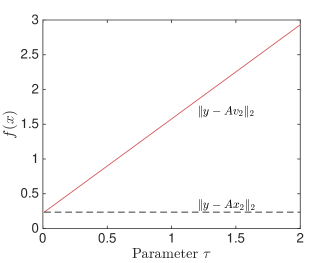
Refer to caption
Figure 4. The use of momentum could be skipped in [33].

Here, we present a toy example for the analysis in [33], where momentum term is not guaranteed to be used per step. While this is not in general an issue, it might lead to repeatedly skipping the momentum term and, thus losing the acceleration.

Let us focus on the sparse linear regression problem, where the analysis in [33] applies. That means, f(x):=bΦx22assign𝑓𝑥superscriptsubscriptnorm𝑏Φ𝑥22f(x):=\|b-\Phi x\|_{2}^{2}, where bm𝑏superscript𝑚b\in\mathbb{R}^{m}, Φm×nΦsuperscript𝑚𝑛\Phi\in\mathbb{R}^{m\times n} and xn𝑥superscript𝑛x\in\mathbb{R}^{n}. b𝑏b represents the set of observations, according to the linear model: b=Φx+ε𝑏Φsuperscript𝑥𝜀b=\Phi x^{\star}+\varepsilon, where xsuperscript𝑥x^{\star} is the sparse vector we look for and ε𝜀\varepsilon is an additive noise term. We assume that m<n𝑚𝑛m<n and, thus, regularization is needed in order to hope for a meaningful solution.

Similar to the algorithm considered in this paper, [33] performs a momentum step, where vi+1=xi+1+τi+1(xi+1xi),subscript𝑣𝑖1subscript𝑥𝑖1subscript𝜏𝑖1subscript𝑥𝑖1subscript𝑥𝑖v_{i+1}=x_{i+1}+\tau_{i+1}\cdot(x_{i+1}-x_{i}), where

τi+1subscript𝜏𝑖1\displaystyle\tau_{i+1} =argminτbΦvi+122absentsubscriptargmin𝜏superscriptsubscriptnorm𝑏Φsubscript𝑣𝑖122\displaystyle=\operatorname*{arg\,min}_{\tau}\|b-\Phi v_{i+1}\|_{2}^{2}
=argminτbΦ(xi+1+τ(xi+1xi))22absentsubscriptargmin𝜏superscriptsubscriptnorm𝑏Φsubscript𝑥𝑖1𝜏subscript𝑥𝑖1subscript𝑥𝑖22\displaystyle=\operatorname*{arg\,min}_{\tau}\|b-\Phi\left(x_{i+1}+\tau\cdot(x_{i+1}-x_{i})\right)\|_{2}^{2}

The above minimization problem has a closed form solution. However, the analysis in [33] assumes that yΦvi+12yΦxi+12subscriptnorm𝑦Φsubscript𝑣𝑖12subscriptnorm𝑦Φsubscript𝑥𝑖12\|y-\Phi v_{i+1}\|_{2}\leq\|y-\Phi x_{i+1}\|_{2}, i.e., per iteration the momentum step does not increase the function value.

As we show in the toy example below, assuming positive momentum parameter τ0𝜏0\tau\geq 0, this assumption leads to no momentum term, when this is not satisfied. Consider the setting:

[0.38700.1514]=b[0.38160.27260.00770.15981.93640.3908]=Φ[100]=x+[0.00550.0084]=εsubscriptmatrix0.38700.1514absent𝑏subscriptmatrix0.38160.27260.00770.15981.93640.3908absentΦsubscriptmatrix100absentsuperscript𝑥subscriptmatrix0.00550.0084absent𝜀\displaystyle\underbrace{\begin{bmatrix}0.3870\\ -0.1514\end{bmatrix}}_{=b}\approx\underbrace{\begin{bmatrix}0.3816&-0.2726&0.0077\\ -0.1598&1.9364&-0.3908\end{bmatrix}}_{=\Phi}\cdot\underbrace{\begin{bmatrix}1\\ 0\\ 0\end{bmatrix}}_{=x^{\star}}+\underbrace{\begin{bmatrix}0.0055\\ 0.0084\end{bmatrix}}_{=\varepsilon}

Further, assume that x1=[1.733800]subscript𝑥1superscriptmatrix1.733800topx_{1}=\begin{bmatrix}-1.7338&0&0\end{bmatrix}^{\top} and x2=[1.541500]subscript𝑥2superscriptmatrix1.541500topx_{2}=\begin{bmatrix}1.5415&0&0\end{bmatrix}^{\top}. Observe that bΦx12=1.1328subscriptnorm𝑏Φsubscript𝑥121.1328\|b-\Phi x_{1}\|_{2}=1.1328 and bΦx22=0.2224subscriptnorm𝑏Φsubscript𝑥220.2224\|b-\Phi x_{2}\|_{2}=0.2224, i.e., we are “heading" towards the correct direction. However, for any τ>0𝜏0\tau>0, bΦv22subscriptnorm𝑏Φsubscript𝑣22\|b-\Phi v_{2}\|_{2} increases; see Figure 4. This suggests that, unless there is an easy closed-form solution for τ𝜏\tau, setting τ𝜏\tau differently does not guarantee that the function value f(vi+1)𝑓subscript𝑣𝑖1f(v_{i+1}) will not increase, and the analysis in [33] does not apply.

Appendix E More experiments

E.1. Group sparse, 2subscript2\ell_{2}-norm regularized logistic regression

For this task, we use the tumor classification on breast cancer dataset in [62] and test Algorithm 1 on group sparsity model 𝒜𝒜\mathcal{A}: we are interested in finding groups of genes that carry biological information such as regulation, involvement in the same chain of metabolic reactions, or protein-protein interaction. We follow the procedure in [14]999I.e., 5-fold cross validation scheme to select parameters for group sparsity and 2subscript2\ell_{2}-norm regularization parameter - we use β^^𝛽\widehat{\beta} as in subsection 6.1. to extract misclassification rates and running times for FW variants, IHT and Algorithm 1. The groupings of genes are overlapping, which means that exact projections are hard to obtain. We apply the greedy projection algorithm of [14] to obtain approximate projections. For cross-validating for the FW variants, we sweep over {103,102,101,1,10,100}superscript103superscript102superscript101110100\{10^{-3},10^{-2},10^{-1},1,10,100\} for regularization parameter, and {101,1,5,10,50,100}superscript101151050100\{10^{-1},1,5,10,50,100\} for the scaling of the 1subscript1\ell_{1} norm ball for sparsity inducing regularization. For IHT variants, we use the same set for the sweep for regularization parameter as we used for FW variants, and use {2,5,10,15,20,50,75,100}251015205075100\{2,5,10,15,20,50,75,100\} for sweep over the number of groups selected. After the best setting is selected for each algorithm, the time taken is calculated for time to convergence with the respective best parameters. The results are tabulated in Table 1. We note that this setup is out of the scope of our analysis, since our results assume exact projections. Nevertheless, we obtain competitive results suggesting that the acceleration scheme we propose for IHT warrants further study for the case of inexact projections.

Algorithm Test error Time (sec)
FW [8] 0.2938 58.45
FW-Away [8] 0.2938 40.34
FW-Pair [8] 0.2938 38.22
IHT [14] 0.2825 5.24
Algorithm 1 0.2881 3.45
Table 1. Results for 2subscript2\ell_{2}-norm regularized logistic regression for tumor classification on the breast cancer dataset.

E.2. Low rank image completion from subset of entries

Here, we consider the case of matrix completion in low-rank, subsampled images. In particular, let Xp×nsuperscript𝑋superscript𝑝𝑛X^{\star}\in\mathbb{R}^{p\times n} be a low rank image; see Figures 6-7 for some “compressed" low rank images in practice. In the matrix completion setting, we observe only a subset of pixels in Xsuperscript𝑋X^{\star}: b=(X)𝑏superscript𝑋b=\mathcal{M}(X^{\star}) where :p×nm:superscript𝑝𝑛superscript𝑚\mathcal{M}:\mathbb{R}^{p\times n}\rightarrow\mathbb{R}^{m} is the standard mask operation that down-samples Xsuperscript𝑋X^{\star} by selecting only mpnmuch-less-than𝑚𝑝𝑛m\ll p\cdot n entries. The task is to recover Xsuperscript𝑋X^{\star} by minimizing f(X)=12b(X)22𝑓𝑋12superscriptsubscriptnorm𝑏𝑋22f(X)=\tfrac{1}{2}\|b-\mathcal{M}(X)\|_{2}^{2}, under the low-rank model 𝒜𝒜\mathcal{A}. According to [63], such setting satisfies a slightly different restricted strong convexity/smoothness assumption; nevertheless, in Figures 5-7 we demonstrate in practice that standard algorithms could still be applied: we compare accelerated IHT with plain IHT [10], an FW variant [7], and the very recent matrix factorization techniques for low rank recovery (BFGD) [64, 65]. In our experiments, we use a line-search method for step size selection in accelerated IHT and IHT. We observe the superior performance of accelerated IHT, compared to the rest of algorithms; it is notable to report that, for moderate problem sizes, non-factorized methods seem to have advantages in comparison to non-convex factorized methods, since low-rank projections (via SVD or other randomized algorithms) lead to significant savings in terms of number of iterations. Similar comparison results can be found in [12, 29]. Overall, it was obvious from our findings that Algorithm 1 obtains the best performance among the methods considered.
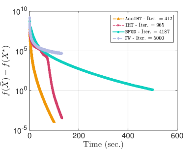
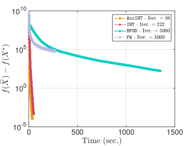
Refer to caption
Refer to caption
Figure 5. Time spent vs. function values gap f(x^)f(x)𝑓^𝑥𝑓superscript𝑥f(\widehat{x})-f(x^{\star}). Left plot corresponds to the “bikes" image, while the right plot to the “children" image.
Refer to caption
Refer to caption
Refer to caption
Refer to caption
Refer to caption
Refer to caption
Refer to caption
Figure 6. Reconstruction performance in image denoising settings. The image size is 512×768512768512\times 768 (393,216393216393,216 pixels) and the approximation rank is preset to r=60𝑟60r=60. We observe 35% of the pixels of the true image. Top row: Original, low rank approximation, and observed image. Bottom row: Reconstructed images.
Refer to caption
Refer to caption
Refer to caption
Refer to caption
Refer to caption
Refer to caption
Refer to caption
Figure 7. Reconstruction performance in image denoising settings. The image size is 683×10246831024683\times 1024 (699,392699392699,392 pixels) and the approximation rank is preset to r=60𝑟60r=60. We observe 35% of the pixels of the true image. Top row: Original, low rank approximation, and observed image. Bottom row: Reconstructed images.