Inverse Classification for Comparison-based Interpretability in Machine Learning
Abstract
In the context of post-hoc interpretability, this paper addresses the task of explaining the prediction of a classifier, considering the case where no information is available, neither on the classifier itself, nor on the processed data (neither the training nor the test data). It proposes an instance-based approach whose principle consists in determining the minimal changes needed to alter a prediction: given a data point whose classification must be explained, the proposed method consists in identifying a close neighbour classified differently, where the closeness definition integrates a sparsity constraint. This principle is implemented using observation generation in the Growing Spheres algorithm. Experimental results on two datasets illustrate the relevance of the proposed approach that can be used to gain knowledge about the classifier.
Introduction
Bringing transparency to machine learning models is nowadays a crucial task. However, the complexity of today’s best-performing models as well as the subjectivity and lack of consensus over the notion of interpretability make it difficult to address.
Over the past few years, multiple approaches have been proposed to bring interpretability to machine learning, relying on intuitions about what ’interpretable’ means and what kind of explanations would help a user understand a model or its predictions. Existing categorizations of interpretability (?; ?; ?; ?) usually distinguish approaches mainly on the characteristics of these explanations: given a classifier to be interpreted, in-model interpretability relies on modifying its learning process to make it simpler (see for instance Abdollahi et al. 2016). Other approaches consist in building a new simpler model to replace the original classifier (?; ?). On the contrary, post-hoc interpretability focuses on building an explainer system using the results of the classifier to be explained.
In this work, we propose a post-hoc approach that aims at explaining a single prediction of a model through comparison. In particular, given a classifier and an observation to be interpreted, we focus on finding the closest possible observation belonging to a different class.
Explaining through particular examples has been shown in cognitive and teaching sciences to facilitate the learning process of a user (see e.g. Watson et al. (2008)). This is especially relevant in cases where the classifer decision to explain is complex and other interpretability approaches cannot provide meaningful explanations. Another motivation for our approach lies in the fact that in many applications of machine learning today, no information about the original classifier or existing data is made available to the end-user, making model- and data-agnostic intepretability approaches essential.
To address these issues we propose Growing Spheres, a generative approach that locally explores the input space of a classifier to find its decision boundary. It has the specifity of not relying on any existing data other than the observation to be interpreted to find the minimal change needed to alter its associated prediction.
The paper is organized as follows: we first present some existing approaches for post-hoc interpretability and how they relate to the one proposed in this paper. Then, we describe the proposed comparison-based approach as well as its formalization and motivations. We then describe the Growing Spheres algorithm. Finally, we illustrate the method through two real-world applications and analyze how it can be used to gain information about a classifier.
Post-hoc Interpretability
Post-hoc interpretability approaches aim at explaining the behavior of a classifier around particular observations to let the user understand their associated predictions, generally disregarding what the actual learning process of the model might be. Post-hoc interpretability of results has received a lot of interest recently (see for instance Kim and Doshi-Velez (2017)), especially as black-box models such as deep neural networks and ensemble models are being more and more used for classification despite their complexity. This section briefly reviews the main existing approaches, depending on the hypotheses that are made about available inputs and on the forms the explanations take. These two axes of discussion, which obviously overlap, provide a good framework for the motivations of our approach.
Available Inputs
Let us consider the case of a physician using a diagnostic tool. It is natural to speculate that (s)he does not have any information about the machine learning model used to make disease predictions, neither may (s)he have any idea about what patients were used to train it. This raises the question of what knowledge (about the machine learning model and the training or other data) an end-user has, and hence what inputs a post-hoc explainer should use.
Several approaches rely specifically on the knowledge of the algorithm used to make predictions, taking advantage of the classifier structure to generate explanations (?; ?). However, in other cases, no information about the prediction model is available (the model might be accessible only through an API or a software for instance). This highlights the necessity of having model-agnostic interpretability methods that can explain predictions without making any hypotheses on the classifier (?; ?; ?). These approaches, sometimes called sensitivity analyzes, generally try to analyze how the classifier locally reacts to small perturbations. For instance, Baehrens et al. (2010) approximate the classifier with Parzen windows to calculate the local gradient of the model and understand what features locally impact the class change.
Forms of Explanations
Beyond the differences regarding their inputs, the variety of existing methods also comes from the lack of consensus regarding the definition, and a fortiori the formalization, of the very notion of interpretability. Depending on the task performed by the classifier and the needs of the end-user, explaining a result can take multiple forms. Interpretability approaches hence rely on the following assumptions to design explanations:
-
1.
The explanations should be an accurate representation of what the classifier is doing.
-
2.
The explanations should be understandably read by the user.
Feature importances (?; ?), binary rules (?) or visualizations (?) for instance give different insights about predictions without any knowledge on the classifier. The LIME approach (?) linearily approximates the local decision boundary of a classifier and calculates the linear coefficients of this approximation to give local feature importances, while Hendricks et al. (2016) identify class-discriminative properties that justify predictions and generate sentences to explain image classification.
In this paper, we consider the case of instance-based approaches, which bring interpretability by comparing an observation to relevant neighbors (?; ?; ?; ?). These approaches use other observations (from the train set, from the test set or generated ones) as explanations to bring transparency to a prediction of a black-box classifier.
One of the motivations for instance-based approaches lies in the fact that in some cases the two objectives and mentioned above are contradictory and cannot be both reached in a satisfying way. In these complex situations, finding examples is an easier and more accurate way to describe the classifier behavior than trying to force a specific inappropriate explanation representation, which would result in incomplete, useless or misleading explanations for the user.
As an illustration, Baehrens et al. (2010) discuss how their approach based on Parzen windows does not succeed well in providing explanations for individual predictions that are at the boundaries of the training data, giving explanation vectors (gradients) actually pointing in the (wrong) opposite direction from the decision boundary. Comparison with observations from the other class would probably make more sense in such a case and give more useful insights.
Existing instance-based approaches moreover often rely on having some prior knowledge, be it about the machine learning model, the train dataset, or other labelled instances. For instance, Kabra et al. (2015) try to identify which train observations have the highest direct influence over a single prediction.
Comparison-based Interpretability
In this section, we motivate the proposed approach in the light of the two axes of discussion presented in the previous section.
Explaining by Comparing
Disposing of knowledge on the classifier or data is an asset existing methods can use to create the explanations they desire. However, the democratization of machine learning implies that in a lot of nowadays cases, the end-user of an explainer system does not have access to any of this knowledge, making such approaches unrealistic. In this context, the need for a comparison-based interpretability tool that does not rely on any prior knowledge, including any existing data, constitutes one of the main motivations for our work.
Due to its highly subjective nature, interpretability in machine learning sometimes looks up to cognitive sciences for a justification for building explanations (when they do not, they rely on intuitive ideas about what interpretable means). Although not mentioned by the previously cited instance-based approaches, it must be underlined that learning through examples also possesses a strong justification in cognitive and teaching sciences (?; ?; ?; ?). For instance, Watson et al. (2008) show through experiences that generated examples help students ’see’ abstract concepts that they had trouble understanding with more formal explanations.
Driven by this cognitive justification and the need to have a tool that can be used when the available information is scarce, we propose an instance-based approach relying on comparison between the observation to be interpreted and relevant neighbors.
Principle of the Proposed Approach
In order to interprete a prediction through comparison, we propose to focus on finding an observation belonging to the other class and answer the question: ’Considering an observation and a classifier, what is the minimal change we need to apply in order to change the prediction of this observation?’. This problem is similar to inverse classification (?), but we apply it to interpretability.
Explaining how to change a prediction can help the user understand what the model considers as locally important. However, compared to feature importances which are often built to have some kind of statistical robustness, this approach does not claim to bring any causal knowledge. On the contrary, it gives local insights disregarding the global behavior of the model and thus differs from other interpretability approaches. For instance, Ribeiro et al. (2016) evaluate their method LIME by looking at how faithful to the global model the local explainer is. However, despite not providing any causal information, the proposed approach provides the exact values needed to change the prediction class, which is also very helpful to the user.
Furthermore, it is important to note that our primary goal here is to give insights about the classifier, not the reality it is approximating. This approach thus aims at understanding a prediction regardless of whether the classifier is right or wrong, or whether or not the observations generated as explanations are absurd. This characteristic is shared with adversarial machine learning (?; ?; ?), which relates to our approach since it aims at ’fooling’ a classifier by generating close variations of original data in order to change their predictions. These adversarial examples rely on exploiting weaknesses of classifiers such as their sensitivity to unknown data, and are usually generated using some knowledge of the classifier (such as its loss function). The approach we propose also relies on generating observations that might not be realistic but without any knowledge about the classifier whatsoever and for the purpose of interpretability.
Finding the Closest Ennemy
For simplification purposes, we propose a formalization of the proposed approach for binary classification. However, it can be applied to multiclass classification.
Let us consider a problem where a classifier maps some input space of dimension to an output space , and suppose that no information is available about this classifier. Suppose all features are scaled to the same range. Let be the observation to be interpreted and its associated prediction. The goal of the proposed instance-based approach is to explain through an other observation . The final form of explanation is the difference vector .
In particular, we focus on finding an observation belonging to a different class than , i.e. such that . For simplification purposes, we call ally an observation belonging to the same class as by the classifier, and ennemy if it is classified to the other class.
Recalling objective mentioned earlier, the final explanation we are looking for should be an accurate representation of what the classifier is doing. This is why we decide to transform this problem into a minimization problem by defining the function such that is the cost of moving from observation to ennemy .
Using this notation, we focus on solving the following minimization problem:
| (1) |
The difficulty of defining the cost function comes from the fact that despite the classifier being designed to learn and optimize some specific loss function, the considered black-box hypothesis compells us to choose a different metric.
Thus, we define as:
| (2) |
with , the weight associated to the vector sparsity and the Euclidean norm.
Looking up to Strumbelj et al. (2009), we choose to use the norm of the vector as a component of the cost function to measure the proximity between and . However, recalling objective , we need to make sure that this cost function guarantees a final explanation that can be easily read by the user. In this regard, we consider that human users intuitively find explanations of small dimension to be simpler. Hence, we decide to integrate vector sparsity, measured by the norm, as another component of the cost function and combine it with the norm as a weighted average.
Due to the cost function being discontinuous and the hypotheses made (black-box classifier and no existing data) solving problem (1) is difficult. Hence, we choose to solve sequentially the two components of the cost function using Growing Spheres, a two-step heuristic approach that approximates the solution of this problem.
Growing Spheres
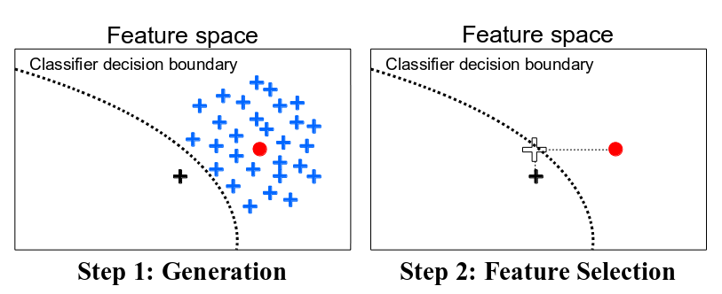
In order to solve the problem defined in Equation (1), the proposed approach Growing Spheres uses instance generation without relying on existing data. Thus, considering an observation to interprete, we ignore in which direction the closest classifier boundary might be. In this context, a greedy approach to find the closest ennemy is to explore the input space by generating instances in all possible direction until the decision boundary of the classifier is crossed, thus minimizing the -component of our metric. This step is detailed in the next part, Generation.
Then, in order to make the difference vector of the closest ennemy sparse, we simplify it by reducing the number of features used when moving from to (thus minimizing the component of the cost function and generating the final solution ), as explained in the Feature Selection part.
An illustration of the two steps of Growing Spheres is drawn in Figure 1.
Generation
The generation step of Growing Spheres is detailed in Algorithm 1. Its main idea is to generate observations in the feature space in -spherical layers around until an ennemy is found. For two positive numbers and , we define a -spherical layer around as:
To generate uniformly over these subspaces, we use the YPHL algorithm (?) which generates observations uniformly distributed over the surface of the unit sphere. We then draw -distributed values and use them to rescale the distances between the generated observations and . As a result, we obtain observations that are uniformly distributed over .
The first step of the algorithm consists in generating uniformly observations in the -ball of radius and center , which corresponds to (line 1 of Algorithm 1), with and hyperparameters of the algorithm.
In case this initial generation step already contains ennemies, we need to make sure that the algorithm did not miss the closest decision boundary. This is done by updating the value of the initial radius: and repeating the initial step until no ennemy is found in the intial ball (lines 2 to 5).
However, if no ennemy is found in , we update and using , generate over and repeat this process until the first ennemy has been found (as detailed in lines 6 to 11).
In the end, Algorithm 1 returns the -closest generated ennemy from the observation to be interpreted (as represented by the black plus in Figure 1).
Once this is done, we focus on making the associated explanation as easy to understand as possible through feature selection.
Feature Selection
Let be the closest ennemy found by Algorithm 1. Our second objective is to minimize the component of the cost function defined in Equation (2). This means that we are looking to maximize the sparsity of vector with respect to . To do this, we consider again a naive heuristic based on the idea that the smallest coordinates of might be less relevant locally regarding the classifier decision boundary and should thus be the first ones to be ignored.
The feature selection algorithm we use is detailed in Algorithm 2.
The final explanation provided to interprete the observation and its associated prediction is the vector , with the final ennemy identified by the algorithms (represented by the white plus in Figure 1).
Experiments
The aforementioned difficulties of working with interpretability make it often impossible to evaluate approaches and compare them one to another.
Some of the existing approaches (?; ?; ?) rely on surveys for evaluation, asking users questions to measure the extent to which they help the user in performing his final task, in order to assess some kind of explanation quality. However, creating reproducible research in machine learning requires to define mathematical proxies for explanation quality.
In this context, we present illustrative examples of the proposed approach applied to news and image classification. In particular, we analyze how the explanations given by Growing Spheres can help a user gain knowledge about a problem or identify weaknesses of a classifier. Additionally, we check that the explanations can be easily read by a user by measuring the sparsity of the explanations found.
Application for News Popularity Prediction
We apply our method to explain the predictions of a random forest algorithm over the news popularity dataset (?). Given 58 numerical features created from 39644 online news articles from website Mashable, the task is to predict wether said articles have been shared more than 1400 times or not. Features for instance encode information about the format and content of the articles, such as the number of words in the title, or a measure of the content subjectivity or the popularity of the keywords used. We split the dataset and train a random forest classifier (RF) on 70% of the data. We use a grid search to look for the best hyperparameters of RF (number of trees) and test it on the rest of the data (0.70 final AUC score). We use to define the cost function and set the hyperparameters of Algorithm 1 to and .
Illustrative Example
We apply Growing Spheres to two random observations from the test set (one from each class). For instance, let us consider the case of an article entitled ’The White House is Looking for a Few Good Coders’ (Article 1). This article is predicted to be not popular by RF.
The explanation vector given by Growing Spheres for this prediction has 2 non-null coordinates that can be found in Table 1: among the articles referenced in Article 1, the least popular of them would need to have 2016 more shares in order to change the prediction of the classifier. Additionally, the keywords used in Article 1 are each associated to several articles using them. For each keyword, the most popular of these articles would need to have 913 more shares in order to change the prediction. In other words, Article 1 would be predicted to be popular by RF if the references and the keywords it uses were more popular themselves.
On the opposite, as presented in Table 2, these same features would need to be reduced for Article 2, entitled ”Intern’ Magazine Expands Dialogue on Unpaid Work Experience’ and predicted to be popular, to change class. Additionally, the feature ’text subjectivity score’ (score between 0 and 1) would need to be reduced by 0.03, indicating that a slightly more objective point of view from the author would lead to have Article 2 predicted as being not popular.
| Feature | Move |
|---|---|
| Min. shares of referenced articles in Mashable | +2016 |
| Avg. keyword (max. shares) | +913 |
| Feature | Move |
|---|---|
| Avg. keyword (max. shares) | -911 |
| Min. shares of referenced articles in Mashable | -3557 |
| Text subjectivity | -0.03 |
Sparsity Evaluation
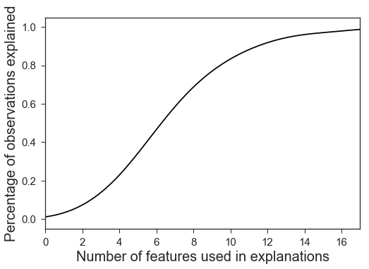
In order to check whether the proposed approach fulfills its goal of finding explanations that can be easily understood by the user, we evaluate the global sparsity of the explanations generated for this problem. We measure sparsity as the number of non-zero coordinates of the explanation vector . Figure 2 shows the smoothed cumulative distribution of this value for all 11893 test data points. We observe that the maximum value over the whole test dataset is 17, meaning that each observation of the test dataset only needs to change 17 coordinates or less in order to cross the decision boundary. Moreover, 80% of them only need to move in 9 directions or less, that is 15% of the features only. This shows that the proposed method indeed achieves sparsity in order to make explanations more readable. It is important to note that this does not mean that we only need 17 features to explain all the observations, since nothing guarantees different explanations use the same features.
This experiment gives an illustration of how this method can be used to gain knowledge on articles popularity prediction.
Applications to Digit Classification
Another application for this approach is to get some understanding of how the model behaves in order to improve it. We use the MNIST handwritten digits database (?) and apply Growing Spheres to the binary classification problem of recognizing the digits 8 and 9. The filtered dataset contains 11800 instances of 784 features (28 by 28 pictures of digits). We use a support vector machine classifier (SVM) with a RBF kernel and parameter . We train the model on 70% of the data and test it on the rest (0.98 AUC score). We use the same values for and the hyperparameters of Algorithm 1 as in the first experiment.
Illustrative Example
Given a picture of an 8 (Figure 3), our goal is to understand how, according to the classifier, we could transform this 8 into a 9 (and reciprocally), in order to get a sense of what parts of the image are considered important. Our intuition would be that ’closing the bottom loop’ of a 9 should be the most influential change needed to make a 9 become an 8, and hence features provoking a class change should include pixels found in the bottom-left area of the digits. Output examples to interprete a 9 and a 8 predictions are shown in Figure 3.
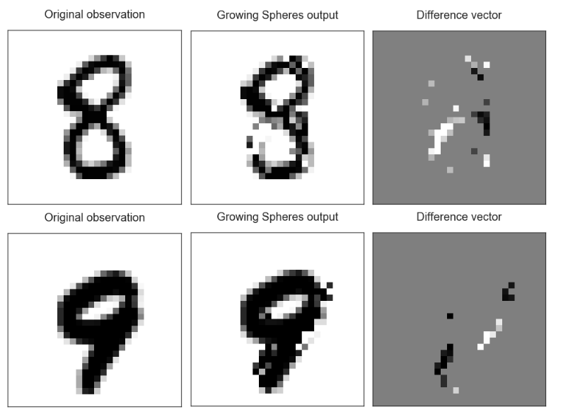
Looking at Figure 3, the first thing we observe confirms our intuition that a good proportion of the non-null coordinates of the explanation vector are pixels located in the bottom-left part of the digits (as seen in pictures right-column pictures). Hence, we can see when comparing left and center pictures that Growing Spheres found the closest ennemies of the original observation by either opening (top example) or closing (bottom example) the bottom part of the digits.
However, we also note that some pixels of the explanation vectors are much harder to understand, such as the ones located on the top right corner of the explanation image for instance. This was to be expected since, as mentioned earlier, our method is trying to understand the classifier’s decision, not the reality it is approaximating. In this case, the fact that the classifier apparently considers these pixels to be influential the classification of these digits could be an evidence of the learned boundary inaccuracy.
Finally, we note that the closest ennemies found by Growing Spheres (pictures in the center) in both cases are not proper 8 and 9 digits. Especially in the bottom example, a human observer would still probably identify the center digit as a noised version of the original 9 instead of an 8. Thus, despite achieving high accuracy and having learned that bottom-left pixels are important to turn a 9 into an 8 and reciprocally, the classifier still fails to understand the actual concepts making digits recognizable to a human.
We also check the sparsity of our approach over the whole test set (3528 instances). Once again, our method seems to be generating sparse explanations since 100% of the test dataset predictions can be interpreted with explanations of at most 62 features (representing 7.9% of total features).
Conclusion and Future Works
The proposed post-hoc interpretability approach provides explanations of a single prediction through the comparison of its associated observation with its closest ennemy. In particular, we introduced a cost function taking into account the sparsity of the explanations, and described the implementation Growing Spheres, which answers this problem when having no information about the classifier nor existing data. We showed that this approach provides insights about the classifier through two applications. In the first one, Growing Spheres allowed us to gain meaningful information about features that were locally relevant in news popularity prediction. The second application highlighted both strengths and weaknesses of the support vector machine used for digits classification, illustrating what concepts were learned by the classifier. Furthermore, we also checked that the explanations provided by the proposed approach are indeed sparse.
Beside collaborating with experts of industrial domains for explanations validation, outlooks for our work include focusing on the constraints imposed to the Growing Spheres algorithm. In numerous real-world applications, the final goal of the user may be such that it would be useless for him to have explanations using specific features. For instance, a business analyst using a model predicting whether or not a specific customer is going to make a purchase would ideally have an explanation based on features that he can leverage. In this context, forbidding the algorithm to generate explanations in specific areas of the input space or using specific features is a promising direction for future work.
References
- [Abdollahi and Nasraoui 2016] Abdollahi, B., and Nasraoui, O. 2016. Explainable Restricted Boltzmann Machines for Collaborative Filtering. ICML Workshop on Human Interpretability in Machine Learning (Whi).
- [Adler et al. 2017] Adler, P.; Falk, C.; Friedler, S. A.; Rybeck, G.; Scheidegger, C.; Smith, B.; and Venkatasubramanian, S. 2017. Auditing black-box models for indirect influence. Proceedings - IEEE International Conference on Data Mining, ICDM 1–10.
- [Angelino et al. 2017] Angelino, E.; Larus-Stone, N.; Alabi, D.; Seltzer, M.; and Rudin, C. 2017. Learning Certifiably Optimal Rule Lists for Categorical Data. Proceedings of the 23rd ACM SIGKDD International Conference on Knowledge Discovery and Data Mining 35–44.
- [Baehrens et al. 2009] Baehrens, D.; Schroeter, T.; Harmeling, S.; Kawanabe, M.; Hansen, K.; and Mueller, K.-R. 2009. How to Explain Individual Classification Decisions. Journal of Machine Learning Research 11:1803–1831.
- [Barbella et al. 2009] Barbella, D.; Benzaid, S.; Christensen, J.; Jackson, B.; Qin, X. V.; and Musicant, D. 2009. Understanding Support Vector Machine Classifications via a Recommender System-Like Approach. Proceedings of the International Conference on Data Mining 305–11.
- [Bibal 2016] Bibal, A. 2016. Interpretability of Machine Learning Models and Representations : an Introduction. ESANN 2016 proceedings, European Symposium on Artificial Neural Networks, Computational Intelligence and Machine Learning (April):77–82.
- [Biran and Cotton 2017] Biran, O., and Cotton, C. 2017. Explanation and Justification in Machine Learning : A Survey. International Joint Conference on Artificial Intelligence Workshop on Explainable Artificial Intelligence (IJCAI-XAI).
- [Decyk 1994] Decyk, B. N. 1994. Using Examples to Teaching Concepts. In Changing College Classrooms: New teaching and learning strategies for an inscreasingly complex world. 39–63.
- [Doshi-Velez and Kim 2017] Doshi-Velez, F., and Kim, B. 2017. Towards A Rigorous Science of Interpretable Machine Learning. 1–12.
- [Fernandes, Vinagre, and Cortez 2015] Fernandes, K.; Vinagre, P.; and Cortez, P. 2015. A proactive intelligent decision support system for predicting the popularity of online news. In Lecture Notes in Computer Science (including subseries Lecture Notes in Artificial Intelligence and Lecture Notes in Bioinformatics), volume 9273, 535–546.
- [Goodfellow, Shlens, and Szegedy 2015] Goodfellow, I. J.; Shlens, J.; and Szegedy, C. 2015. Explaining and Harnessing Adversarial Examples. In International Conference on Learning Representation.
- [Harman and Lacko 2010] Harman, R., and Lacko, V. 2010. On decompositional algorithms for uniform sampling from n-spheres and n-balls. Journal of Multivariate Analysis 101(10):2297–2304.
- [Hendricks et al. 2016] Hendricks, L. A.; Akata, Z.; Rohrbach, M.; Donahue, J.; Schiele, B.; and Darrell, T. 2016. Generating visual explanations. Lecture Notes in Computer Science (including subseries Lecture Notes in Artificial Intelligence and Lecture Notes in Bioinformatics) 9908 LNCS:3–19.
- [Kabra, Robie, and Branson 2015] Kabra, M.; Robie, A.; and Branson, K. 2015. Understanding classifier errors by examining influential neighbors. In Proceedings of the IEEE Computer Society Conference on Computer Vision and Pattern Recognition, volume 07-12-June, 3917–3925.
- [Kim and Doshi-Velez 2017] Kim, B., and Doshi-Velez, F. 2017. Interpretable Machine Learning : The fuss , the concrete and the questions. In ICML Tutorial on interpretable machine learning.
- [Krause, Perer, and Bertini 2016] Krause, J.; Perer, A.; and Bertini, E. 2016. Using Visual Analytics to Interpret Predictive Machine Learning Models. ICML Workshop on Human Interpretability in Machine Learning (Whi):106–110.
- [Lakkaraju and Rudin 2017] Lakkaraju, H., and Rudin, C. 2017. Learning Cost-Effective and Interpretable Treatment Regimes. Proceedings of the 20th International Conference on Artificial Intelligence and Statistics 54(3):166–175.
- [LeCun et al. 1998] LeCun, Y.; Bottou, L.; Bengio, Y.; and Haffner, P. 1998. Gradient-based learning applied to document recognition. Proceedings of the IEEE 86(11):2278–2323.
- [Mannino and Koushik 2000] Mannino, M. V., and Koushik, M. V. 2000. The Cost Minimizing Inverse Classification Problem : a Genetic Algorithm Approach. Decision Support Systems 29(3):283–300.
- [Martens and Provost 2014] Martens, D., and Provost, F. 2014. Explaining Data-Driven Document Classifications. Mis Quarterly 38(1):73–99.
- [Mvududu and Kanyongo 2011] Mvududu, N., and Kanyongo, G. Y. 2011. Using real life examples to teach abstract statistical concepts. Teaching Statistics 33(1):12–16.
- [Ribeiro, Singh, and Guestrin 2016] Ribeiro, M. T.; Singh, S.; and Guestrin, C. 2016. Why Should I Trust You? Proceedings of the 22nd ACM SIGKDD International Conference on Knowledge Discovery and Data Mining - KDD ’16 39(2011):1135–1144.
- [Štrumbelj, Kononenko, and Robnik Šikonja 2009] Štrumbelj, E.; Kononenko, I.; and Robnik Šikonja, M. 2009. Explaining instance classifications with interactions of subsets of feature values. Data and Knowledge Engineering 68(10):886–904.
- [Szegedy et al. 2014] Szegedy, C.; Zaremba, W.; Sutskever, I.; Bruna, J.; Erhan, D.; Goodfellow, I.; and Fergus, R. 2014. Intriguing properties of neural networks. International Conference on Learning Representation.
- [Turner 2016] Turner, R. 2016. A model explanation system. IEEE International Workshop on Machine Learning for Signal Processing, MLSP 2016-November:1–5.
- [Tygar 2011] Tygar, J. D. 2011. Adversarial machine learning. In IEEE Internet Computing, volume 15, 4–6.
- [van Gog, Kester, and Paas 2011] van Gog, T.; Kester, L.; and Paas, F. 2011. Effects of worked examples, example-problem, and problem-example pairs on novices’ learning. Contemporary Educational Psychology 36(3):212–218.
- [Watson and Shipman 2008] Watson, A., and Shipman, S. 2008. Using learner generated examples to introduce new concepts. Educational Studies in Mathematics 69(2):97–109.