Unifying Map and Landmark Based Representations for Visual Navigation
Abstract
This works presents a formulation for visual navigation that unifies map based spatial reasoning and path planning, with landmark based robust plan execution in noisy environments. Our proposed formulation is learned from data and is thus able to leverage statistical regularities of the world. This allows it to efficiently navigate in novel environments given only a sparse set of registered images as input for building representations for space. Our formulation is based on three key ideas: a learned path planner that outputs path plans to reach the goal, a feature synthesis engine that predicts features for locations along the planned path, and a learned goal-driven closed loop controller that can follow plans given these synthesized features. We test our approach for goal-driven navigation in simulated real world environments and report performance gains over competitive baseline approaches.
1 Introduction
As humans we are able to effortlessly navigate through environments. We can effectively plan paths, find shortcuts and adapt to changes in the environment while only having a relatively coarse sense of the exact geometry of the environment or the exact egomotion over long distances.
Human representations for space [34] start out from destination knowledge, which is a set of places of interest. This guides acquisition of route knowledge that is knowledge of specific routes to go from one destination to another. Already at this point, humans exhibit an impressive ability to follow routes reliably in the presence of changes in the environment (demolition and construction of new buildings, appearance variations due to change in seasons, and the time of day) as well as the uncertainty in their own estimate of their egomotion and location in space. This is facilitated by the use of distinctive landmarks (such as clock towers) that are invariant to changes in the environment and provide visual fixes to collapse the uncertainty in location. As more and more of such route knowledge is experienced over time, it is assimilated into survey knowledge, which is knowledge of the spatial layout of different places and routes with respect to one another. It is at this point that humans are also able to plan paths to novel places and find shortcuts for going between different known points. This is generally accomplished by reasoning over a coarse spatial layout of places through a cognitive map [33].
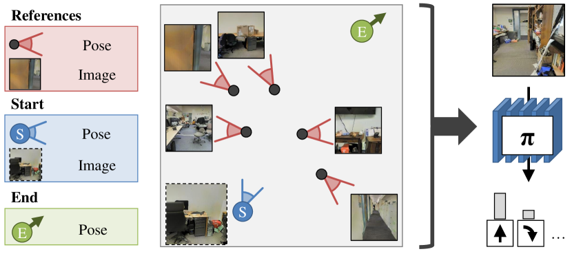
This remarkably human navigation ability is driven by both map based and landmark based representations. Map based representations allow for planning paths and finding shortcuts, while landmark based visual memory of the environment permits executing the planned path in the presence of noisy and uncertain motion. At the same time, humans use their prior experience with other similar environments to construct reasonable path plans with only partial knowledge of a new environment.
Of course, there is vast literature in robotics that studies navigation. Classical approaches employ purely geometric reasoning. This provides accurate geometry, but does not explicitly reason about the semantic distinctiveness of landmarks. At the same time, there is a strict requirement of being able to always localize the agent in this map. Not only is this localization solely driven by geometry, precise localization may not even be always possible (such as in long texture-less hallways). More crucially, classical approaches rely entirely on observed evidence and do not use priors and experience from similar other environments to make meaningful inferences about unobserved parts of the environment.
Contemporary learning based approaches [37, 23] have focused on incorporating such statistical priors, but have largely ignored the question of representation of spaces by making it completely implicit in the form of neural network activations. Works that do build spatial representations (such as [12]), operate under ideal world assumptions where the agent is always aware of its exact location in the environment.
In this work, we build map and landmark based representations for spaces: map based representations are used to plan paths and find shortcuts, while past visual memories are used to derive visual fixes (landmarks) to reliably follow planned paths under noisy actuation. We start by generalizing the cognitive mapping and planning work from Gupta et al. [12] to work with sparse distributed observations of an environment. Next, instead of explicitly localizing with respect to the map at each time step (to read out the next action), we compile a given path plan into a ‘path signature’, comprising the model’s expectation about what the agent will see along the path in addition to the planned actions. This path signature, along with the current observation, is used with a learned policy for closed-loop control to output actions that follow the planned path robustly. If the robot doesn’t see the features it expected, it can take corrective actions without explicit relocalization or replanning. While this approach is quite feasible even with standard geometric mapping and planning methods, our learning-based framework makes it particularly effective: we can express path plans semantically (e.g., go through the door, turn at the end of the corridor), as well as, learn to produce good path signatures for the end task of robust path following. Finally, all parts of our representation are learned from data in an end-to-end manner for the sub-tasks of path planning and path following. This allows us to use prior experience with similar other environments to make meaningful extrapolations, allowing our policies to operate well even with only partial observation of novel environments.
Our experiments in simulated environments (based on reconstructions of real world offices) with simple discrete actions, demonstrate the role of past visual memories for robust plan execution in presence of noisy actuation, and the utility of our specialized policy architectures over standard memory-based neural network architectures.
2 Related Work
There are multiple different branches of research in classical and learning based robotics that tackle the problem of robot navigation. We describe some major efforts here. Robotic navigation research can be broadly categorized along two dimensions: planning-based versus reactive, and learning-based versus geometric. Many of the most popular classical method are planning-based and geometric, and rely on separating mapping and estimation from decision making. Indeed, these two problems are often studied in isolation in robotics [30], as we will discuss below. Most learning-based methods for navigation have been reactive in nature, bypassing the explicit construction of maps or planning. In contrast, our method is both learning-based and planning-based: we combine end-to-end training with explicit construction of spatial representations and planning.
Classical Methods for Navigation.
There is rich literature in various aspects of navigation covering construction of maps from sensory measurements like images and range scans, localization in such maps through probabilistic state estimation, and path planning with noisy actuation. We summarize a few works here, and a comprehensive review appears in [32].
Filtering and estimation methods deal with the problem of estimating the robot’s pose given a history of its sensor readings, typically in a known map that is purely geometric. Methods like particle filtering maintain a probability distribution over the robot’s location and update this distribution based on a generative model of the sensors [8]. Extending this to the setting of unknown environments, simultaneous localization and mapping (SLAM) algorithms [7, 10, 9, 19, 13] aim to both construct a map and localize the robot. These methods are solely focused on constructing maps that are purely geometric and entirely ignore semantics. Odometry and localization methods based on computer vision sometimes also aim to localize the robot without explicitly constructing a map. The most common class of such methods is visual odometry [24, 36], where the goal is to estimate camera motion based on sequences of images in order to determine displacement from a starting point. Standard robotic navigation methods typically decouple mapping or localization from decision making. Once localization has been performed, the action might be determined by a path planning procedure. Many path planning methods [5, 16, 21] assume direct access to a noiseless map, and often a noiseless robot location. A number of methods also incorporate uncertainty, by feathering the obstacles in the environment by the maximum amount of uncertainty to obtain provably safe plans [3].

Given such a constructed map and plan, robot motion happens using a control loop that 1) executes the first action of the plan, 2) relocalizes the robot in the map using new observations, 3) replans to compute optimal action from the new state to the goal location. This control loop crucially depends on being able to accurately relocalize the robot at every time step. Such accurate relocalization is problematic when the environment is featureless (a long texture less hallway) or if it changes (chairs are moved around); or if it becomes necessary to explore new routes. Moreover, all steps in this control loop are entirely based on geometry; and state estimation and action execution are entirely decoupled. Being purely geometric makes this control loop extremely brittle. Furthermore, decoupled estimation and execution makes it impossible to adapt the perception and localization systems to the final task performance. Our work addresses these issues by framing localization as an implicit learning problem thereby allowing use of geometric as well as semantic cues. At the same time, our control loop is entirely learned. This allows for specialization of the implicit localization module for action execution.
Researchers have also looked at view based maps [20] that store views at different locations instead of geometric maps. Such methods directly tie action execution to sensors without learning. This requires maintain enormous collections of images and leads to policies that entirely limited to previously traversed paths.
Learning based Navigation.
Inspired by the short comings of pipelined approaches, there is an increasing focus on end-to-end learned task-driven architectures for robotic applications [22]. Most such approaches [26, 28, 15, 11, 6] study task-agnostic collision avoidance, and don’t build representations for spaces or plan paths. Even task-driven approaches such as [37, 23, 4] either rely only on statistical priors for spaces via learned reactive policies or only build implicit representations in the form of vanilla LSTM memory. Such implicit representations fail to quickly adapt to new environments. In contrast to the above methods, techniques based on learned map construction [12, 25, 17, 35] and value iteration networks [31] have sought to directly incorporate elements of mapping and planning into end-to-end trained navigational policies. These prior methods are closest to our approach. However, they only study the simplified problem without any noise in actuation. This entirely side-steps the problem of localization in the map. We adopt their general paradigm of mapping and planning but extend it to work with only a small set of sparse views. More importantly, we study the problem in the more challenging setting where there is actuation noise. This limits the utility of maps and plans, and we propose techniques to tackle this by unifying landmark based visual fixes to compensate for noisy in actuation.
Another related line of work is learning from demonstration [29] and imitation learning where a policy is trained to follow a given demonstration or observation sequence. Such approaches rely on an external expert to demonstrate the desired behavior at test time and additionally also require actual or close to actual observations that will be encountered while executing the trajectory. In contrast, our work neither requires expert demonstrations nor actual exact images that will be seen when we execute the trajectory.
3 Approach

In this work, we are interested in building representations for spaces starting from visual observations. Let us consider an embodied agent that has some small amount of experience with a novel environment. This experience is in the form a small number (say ) of registered RGB images () along with associated poses (). We denote this set of registered images by . Given this experience with the environment, we want to build representations for this environment that enable this agent to quickly accomplish navigation goals under noisy actuation (i.e. the actions executed by the agent don’t always have the exact intended effect). In particular, given current observations from on-board sensors (RGB image from first person camera) and the compiled representation for space, we want the agent to get to a specified point in space.
Our method is based on two main components: a) a spatial representation that allows path planning and shortcut inference and b) a goal-driven closed-loop controller that executes the plan under noisy actuation. For the former, we adopt and generalize the learning based mapping and planning paradigm from Gupta et al. [12] to operate with a small number of sparse views () of the environment. For the latter, our key insight is that a plan should not just consist of a sequence of actions that will reach the goal, but a ‘path signature’ that additionally also describes the features that the agent expects to see on the way to the goal. This path signature can then be used for closed-loop control: if the robot doesn’t see the features it expected, the agent can use relatively simple, local, error correction strategies to take corrective actions without explicit relocalization and replanning.
Our approach is summarized in Figure 2 and consists of four parts: a) a learned mapper that produces spatial representations of the world given sparse views of the environment; b) a learned path planner that processes the produced map along with the target position to predict optimal paths and guides the learning of the mapper; c) a learned feature synthesizer that hallucinates features at locations along the predicted path using the available sparse views from the environment; and d) a learned control policy that executes the plan based on the hallucinated features and the current first person observation under noisy actuation.
Our approach is reminiscent of classic robotics pipelines, but with the crucial distinction that, instead of using geometry-based, hand-defined, isolated modules, we propose a differentiable, end-to-end trainable, data-driven formulation. This addresses some of the fundamental challenges with standard, geometric localization and planning methods. Classical approaches are driven entirely by explicit geometry and have no way to incorporate statistical priors. They also require design of intermediate representations such as: What should the output of the mapper be? What constitutes a landmark? What features will be useful for matching the current observation to a previously observed landmark or how to decide that a landmark has been reached. Such intermediate representations are hard to design and even harder to optimize given surrogate metrics that do not always correlate with the final performance. Finally, independent modules are usually unaware of the error statistics of the other modules and hence cannot be robust to them.
In contrast, in our proposed formulation, learning allows use of statistical priors based on knowledge of similar other environments; enabling our method to work with only a handful of images. Moreover, joint optimization of modules alleviates the need to hand define intermediate representations that bottleneck the final performance. Furthermore, modules can be trained together, allowing them to be robust the error-modes of one another. We now describe the design of each module.
3.1 Map Generation
The task of our map generator is to transform the registered images to a spatial map that can be used for path planning. Going from images to a common spatial representation facilitates path planning and shortcut finding. Unlike a classical mapper, our proposed mapper is not constrained to output free or occupied space but only a representation that allows for effective path planning. The only structure that we impose is that it is spatial representation i.e. locations in the map correspond to locations in the world. The mapper is free to output arbitrary abstract feature vectors as long as they allow a planner to output meaningful plans.
Given the registered image samples , the mapping function generates the overhead map as follows:
| (1) | |||||
| (2) | |||||
| (3) |
is generated using an encoder/decoder network that learns to transform from the first person view to an egocentric top view of the environment at location . The encoder is composed of convolutional layers that map from raw image pixels to abstract representation for the scene. This representation is transformed through fully connected layers into a top-view that is upsampled by upconvolutional layers to produce feature vectors in an egocentric spatial top view of the world () for each image . These egocentric top-view predictions are transformed into a common allocentric view (i.e. in the world coordinate frame) through a geometric transform determined by the image’s pose to generate . This transform is implemented differentiably using spatial transformers [14]. Different allocentric predictions are accumulated by a function (realized through weighted averaging) and finally upsampled by function using deconvolutions. The map generator transforms the input image observations into an allocentric representation of the world. This allocentric representation of the world can be plugged into downstream modules and optimized jointly.
3.2 Path Planning
Given the abstract spatial map, the task of the planner is to output a path (sequence of actions) that can convey the robot to a desired and known goal location. We are working with abstract spatial representations (i.e. not explicitly free-space), a classical planner can no longer be used. Instead, we learn a planner from data. Given the map in the top-view, we employ a value iteration based planning method to plan a path from the starting location to the goal location. We express value iteration as a convolutional network with max pooling across channels [31] and directly train the planner and the mapper to output the optimal action at different locations in the map [12]. We read off the entire sequence of actions () along the path that convey the robot to the goal location by following optimal actions from the starting location to the goal location. This action sequence can be converted into a sequence of robot poses in the environment.
Formulating mapping and path planning as learning problems allows us to fuse observations of the current environment with statistical knowledge about layout of similar other environments. This lets us meaningfully extrapolate and make predictions about regions of space where no direct observations may have been made. We can thus plan paths in new environments given only a handful of images at sparse locations, and generate more efficient paths than are possible from only the sparse observations.
3.3 Path Signatures
The sequence of planned actions ( and ) is by itself not enough to execute the trajectory in the environment because of noisy actuation: actions executed by the agent will not lead to the same consistent outcome because of environmental noise, slip in motors and uneven terrain. This makes open loop replay of plans problematic because errors compound over time and the location drifts: the agent will execute the optimal plan for the wrong location making its location error worse and worse. Such drift in estimate of one’s location also occurs in humans and animals as they move around and is compensated for by use of visual fixes by re-orienting oneself with respect to a previously known distinctive location. We thus compensate for drift by augmenting the sequence of actions and poses with visual anchors at that location. These feature anchors provide a reference to the agent allowing it to estimate and correct for its drift.
Unfortunately, we may not have explicitly been at in the past and may not have the actual features for that location. To address this we synthesize features for location . We do this using observed features from neighboring points in space that the agent did visit in the past and thus has some features for it.
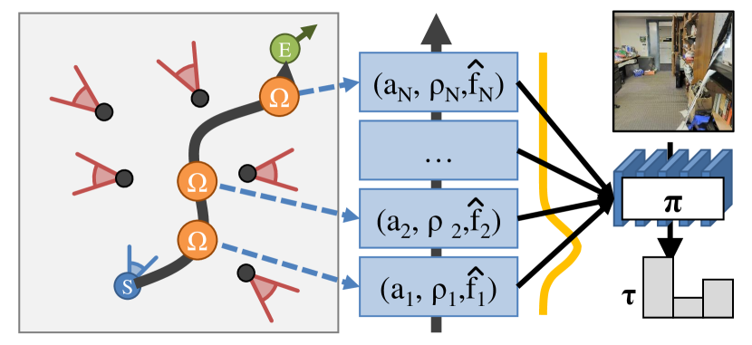
Thus for each location along the plan we have the action, the location and the synthesized features i.e. the tuple . We call the sequence of these tuples a signature of the path that we want the robot to follow:
| (4) |
We next describe how to synthesize features for a location using observation from neighboring locations:
| (5) | |||||
| (6) |
Here, the function computes the relative pose of image with respect to the desired synthesis location . computes representation for image through a CNN followed by two fully connected layers. fuses the relative pose with the representation for the image to obtain the contribution of image towards representation at location . These contributions from different images are accumulated through a weighted addition by function , to obtain the synthesized feature at pose . This, as well as the plan execution module , is depicted in Figure 4.
3.4 Plan Execution
Given a path signature that has the local information needed to follow the trajectory in the environment, we need a policy that can execute this path under noisy actuation.
This learned policy takes the environment and goal specific path signature as input. This factorization of the environment and goal specific information into a path signature that is separate from the policy lets us learn a single policy that can do different things in different environments with different path signatures without requiring any re-training or adaptation. The policy can then also be thought of as a robust closed-loop goal-oriented controller.
We train this policy to follow path under noisy actuation in the environment given current first person views from on-board robot cameras. We represent policy with a recurrent neural network that iterates over the path signature as the agent moves through the environment. This iteration is implemented using sequential soft attention that traverses over the trajectory signature. At each step, the path signature is read into with differentiable soft attention centered at :
| (7) |
The recurrent function with state is implemented as:
| (8) | |||||
| (9) |
As input, it takes the internal state, , attended path signature and featurized image observation . In return, it gives a new state , pointer increment , and action that the agent should execute. This pointer increment is added, after a sigmoid to yield the new pointer . We set and . Our experiments show that this use of sequential reasoning here is critical for performance.
4 Experiments
We describe experiments to evaluate our proposed representation for space for the task of visual navigation. We present a factored evaluation: we evaluate the individual modules, and the two coupled modules (mapping and planning modules together, and path signature and execution modules together). Such a factored evaluation helps us evaluate the design choices for each module without conflating the error modes of different modules.
The goal of the experiment section is to answer the following questions: given only a handful of registered images in a novel environment and under noisy actuation: (1) how well mapping and planning work; (2) to what extent can features for novel locations be predicted; (3) how well can a given trajectory plan be executed; (4) whether visual memory is helpful; and (5) how different architectures for visual memory compare against each other?
Experimental Setup.
Our goal is to enable robot mobility in indoor environments. It is challenging to conduct thorough and controlled experimentation with physical robots. Thus, we use environments that are simulated, but are derived from reconstructions of real buildings (Matterport scans [1]). These environments retain many of the challenges of the real world, such as clutter and realistic appearance, but allow for controlled experiment and systematic analysis.
We use the Stanford Large-Scale 3D Indoor Spaces Dataset [2]. This dataset contains 3D scans of multiple different buildings on the Stanford campus, in the form of textured meshes that can be rendered from arbitrary viewpoints, and has been used for studying navigation tasks [12]. We follow the standard splits for our experiments, using areas 1, 5, 6 for training, area 3 for validation, and area 4 for testing. This ensures that testing is done in a different building from ones used for training and validation. We adapt the publicly available simulation environment from Gupta et al. [12] for our experiments.
4.1 Mapping and Planning
Mapping.
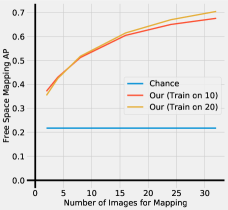
We first study how well our approach can generate maps given a small number of images from a novel environment. We first study this in isolation by training the mapper described in Section 3.1 to predict free space in an environment. Note that this experiment aims only to establish that the mapper architecture is sufficiently expressive; in all other experiments, it is trained end-to-end by backpropagating gradients from upstream modules.
We sample a small number of images with their pose over the area in consideration ( in our experiments) and train the mapper to predict free space over the entire area. We benchmark the performance of this mapper in the test environment and measure the average precision for the task of free space prediction. Our mapper can take a varying number of images as input; we plot performance as a function of the number of test-time images in Figure 5 (far left). Even though the mapper was trained with a fixed number of images ( or ) as input, it works well when tested with different numbers.
Mapping and Planning.
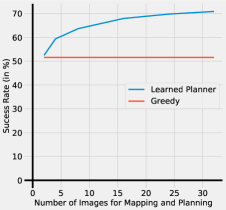
We next study how well paths can be planned with sparse observations. We use the joint mapper and planner architecture described in Sections 3.1 and 3.2 and train it for the task of going to a particular point in space up to 20 steps away within areas of size . As previously described, the mapper and planner generates a spatial map and uses value iteration to output optimal actions to convey the robot to the goal from different locations in the map.
Our goal here is to evaluate only the ability of this system to generate good plans from sparse observations. Therefore, we evaluate how well the plans can be open-loop executed under the assumption of no noise or feedback. We randomly sample start and goal positions and measure the plan execution rate if we simply apply the sequences of actions starting from the start state. Figure 5 (center left) show the success rate as we vary the number of reference images. Again we see performance improves as more and more images are available from the environment.
It is important to note that these representations and path plans are obtained from a small number of RGB images with a limited field of view (). Classical methods rely on being able to compute correspondences between images to reconstruct the world. In our setup, there is a very limited overlap between the different images and such methods simply do not work. Similar experiments were reported by Gupta et al. in [12]. However, Gupta et al. were studying the problem of online mapping and planning and thus, their analysis was limited to streams of consecutive images along a path. Dense observations lead them to develop an egocentric representations and permitted re-planning as new observations came in. In contrast, our experiment here studies the case where only sparse image observations are available. We thus maintain an allocentric representation but show that good path plans can be generated even with sparse observations of the environment. Additionally, in this experiment we are studying the open loop performance of such plans. This is in contrast to the experiments reported in Gupta et al. that only reported the performance of closed loop plans.

4.2 Path Signatures and Execution
We now study feature synthesis for unseen locations from nearby locations, and their use for robustly executing planned trajectories.
Feature Synthesis.
We first analyze feature synthesis for novel points in isolation. This serves as a test bed to evaluate the expressiveness of the feature synthesis architecture.
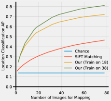
For this evaluation, we train the synthesizer to do localization at novel locations: given the set of images in an area (), we predict features at different target locations using the architecture described in Section 3.3. We train the synthesizer discriminatively for the task of pairing synthesized features at location to actual features at location . We use a multi-layer perceptron classifier on to predict if they are from nearby locations (as determined by the distance between and ), for a number of different pairs of and .
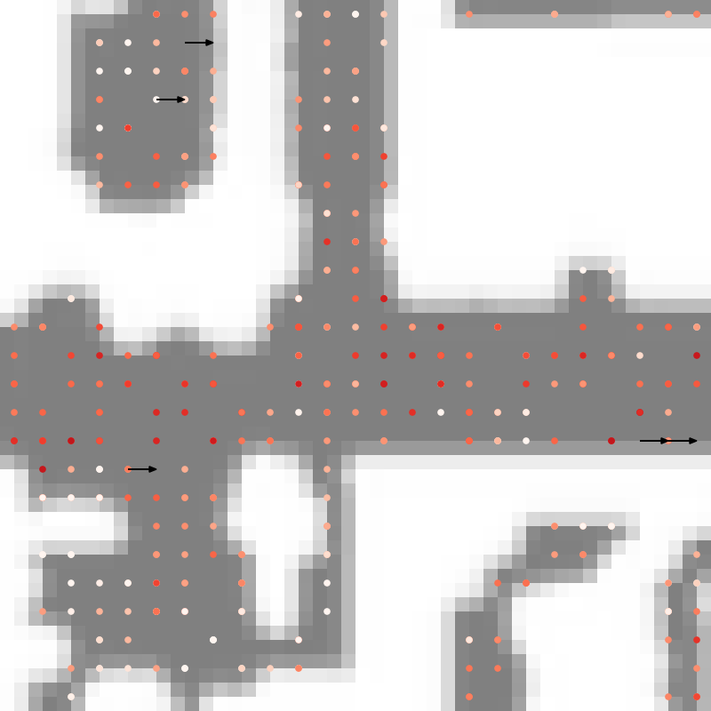
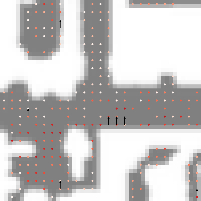
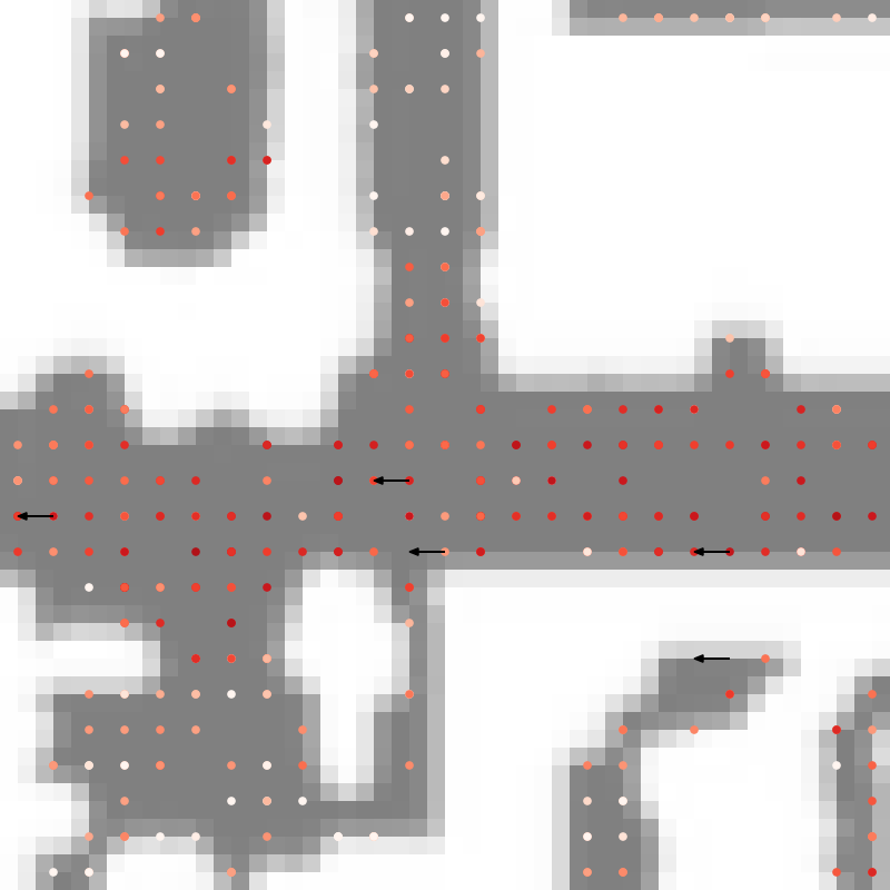
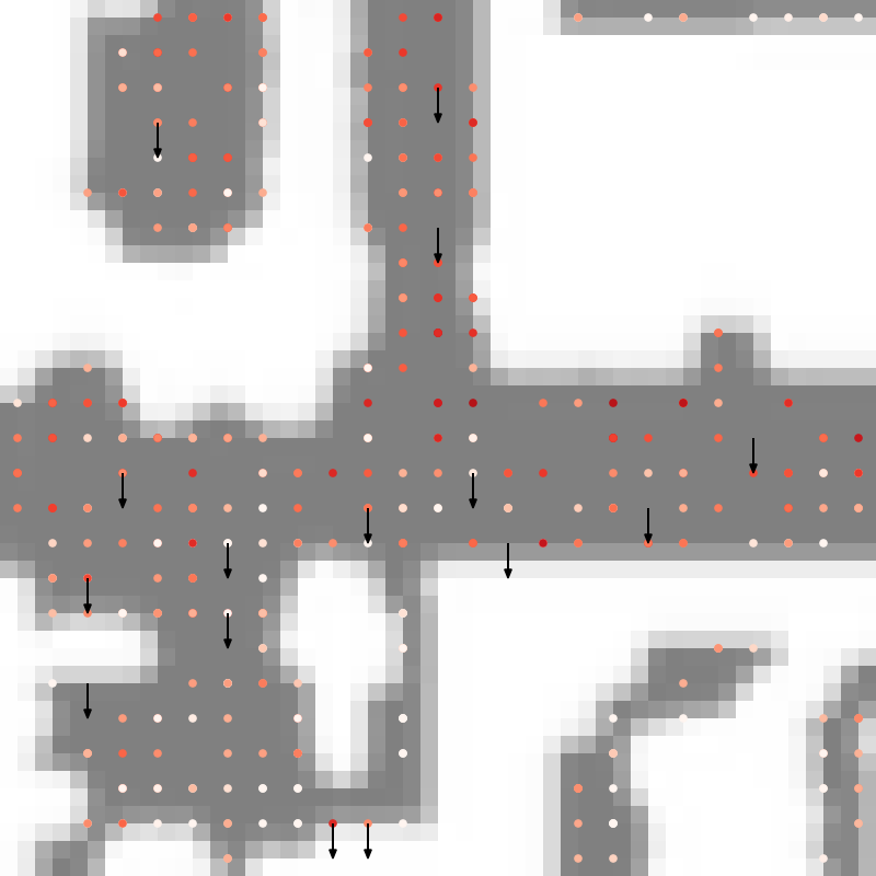
We report the average precision for this classification task in Figure 5 (center right). Note that this network can take a varying number of registered reference images as input, and we plot the performance as a function of the number of reference images. We compare to a SIFT matching based baseline (checking consistency of SIFT keypoint matches with the essential matrix derived from the relative pose between the two images). Our learned features outperform the SIFT baseline. Figure 6 show visualizations for the quality of feature prediction at different locations for a representative prediction, and Figure 7 shows the contribution of different locations towards predicting features at a canonical position (at origin looking upwards).
Path Signatures and Plan Execution.
We now evaluate the design of our architecture for executing planned trajectories. In addition to the set of registered images (), we are given a plan (in the form of sequence of actions and locations in space), that we want the agent to successfully execute. To not conflate with errors in planning, we conduct this experiment with optimal plans for reaching a target point in space (sampled to be between 16 and 18 steps away).
We make some additional modeling assumptions: we use a relatively simple action representation (four discrete actions: stay in place, rotate left by , rotate right by and move forward by ). We simulate noise in actuation by making the move forward action fails with probability. The agent stays in place when the action fails.
Training Details.
We train our policy from Section 3.4, using DAGGER [27], an imitation learning algorithm. We supervise the agent using the optimal action for reaching the goal from the agent’s actual current state (known in the simulator). We found it useful to include an auxiliary loss between the features of the actual observation from location and the predicted features at that location, and slowly switching from to for computing the path signatures as the training proceeded. We also found that using a shallow 5-layer CNN (with strided convolutions for down-sampling instead of max pooling) to represent images led to better performance than using an ImageNet pre-trained ResNet-18 network. We believe strided convolutions and slower down-sampling in our custom network eases learning of pose sensitive representations for reasoning about view-point and geometric image similarity. Policies were trained using Adam [18] for iterations, and learning rate was dropped every iterations.
Metrics.
Performance is measured by executing all policies for steps and measuring the distance to the goal at end of the execution. Table 1 reports the mean distance to goal, 75th percentile distance to goal, and the success rate (finishing within 3 steps of the goal) over such episodes.
Baselines.
We compare to the following baselines.
Open Loop Execution: This policy is an open loop execution of the planned sequence of actions. It ignores the input image and merely applies the planned action sequence, as is, one action at a time.
Learned Action Execution: Our next comparison point is a policy that is trained to execute the planned trajectory in the environment. This policy has exactly the same architecture as our proposed architecture (Section 3.4) except that the path signature is derived only from the sequence of planned actions (and not the associated synthesized views). At run time, this policy receives the current image observation and the planned action sequence and it outputs the action that the agent should execute in the environment. It can use the feedback from the environment (in form of the new image observation) to adapt to failed actions due to noisy actuation. This is a strong baseline. It can learn sensible patterns such as: it is more likely to turn when facing an obstacles, and it is more likely to turn after exiting a room rather than before exiting the room.
Vanilla GRU Policy: We also experiment with a GRU-based policy where we replace our structured policy network with a vanilla GRU. We extract a fixed length representation for the plan by passing it through a GRU. This fixed length representation along with the current observation is used by the policy GRU to output the action that the agent should take.
Settings.
We also study different settings, in particular, how the visual memories () were chosen. We consider two cases: (1) visual memories are sampled from along the path that the agent needs to follow, and (2) the more challenging case when visual memories are randomly sampled from the environment (40 random images over an area of around the trajectory). Our formulation is agnostic to the choice of these images as it synthesizes the necessary views from whatever ones that are available.
| Mean | 75th%ile | Success | |
| Method | Distance | Distance | %age |
| Initial | 16.0 | 17.0 | 0.0 |
| Open Loop Action Execution | 6.2 | 8.0 | 26.9 |
| Learned Action Execution | 5.1 | 7.0 | 35.7 |
| GRU (5 from path) | 5.1 | 6.0 | 36.5 |
| GRU (10 from path) | 5.0 | 6.0 | 37.9 |
| GRU (all from path) | 4.6 | 6.0 | 43.2 |
| GRU (40 from env) | 5.2 | 7.0 | 35.1 |
| Our (5 from path) | 4.4 | 6.0 | 43.9 |
| Our (10 from path) | 3.8 | 5.0 | 52.7 |
| Our (all from path) | 1.8 | 3.0 | 80.5 |
| Our (40 from env) | 4.8 | 6.0 | 37.4 |
Results.
Results are reported in Table 1. The agent starts 16 steps away from the goal on average. Open loop execution of action takes the agent to 6.2 steps away, succeeding about 27% of the times, showing that simple replay of actions fails under noisy actuation. Learning to execute actions in context of the current observation performs much better, boosting the success rate to 35.7%. This shows the benefit of allowing the policy to adjust according to the observed images. Incorporating visual memory further boosts performance, both when using a vanilla GRU and our proposed architecture. When all visual memories along the path are available, our proposed policy has a success rate of 80% compared to 43% for the vanilla GRU policy. This shows the effectiveness of our proposed architecture over a vanilla GRU. We also studied a setting where images being input to the policy were perturbed (color changes, small affine transforms), while keeping the images used to generate the path signatures fixed. We saw only a minor degradation in performance (73% vs 80% success), showing that such learned policies can be trained to be robust to changes in environment.
We also implemented a nearest neighbor approach that computes similarity of the current observation to views in the path signature. This similarity is then used to pick the optimal action. All operations are implemented in a differentiable manner such that the feature space for nearest neighbor matching can be learned. This nearest neighbor approach worked very well when given all images along the path as input (success rate of 84%), but dramatically failed when only a subset of images were available (success rate between 5% and 12%).
| Mean | 75th%ile | Success | |
|---|---|---|---|
| Method | Distance | Distance | %age |
| Initial | 15.99 | 17.00 | 0.00 |
| Open Loop Plan Execution | 7.61 | 11.00 | 20.34 |
| Learned Plan Execution | 6.93 | 10.00 | 26.65 |
| Our | 6.86 | 9.00 | 26.90 |
| Open Loop Plan Execution (No Noise) | 3.80 | 8.00 | 69.53 |
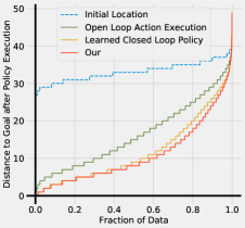
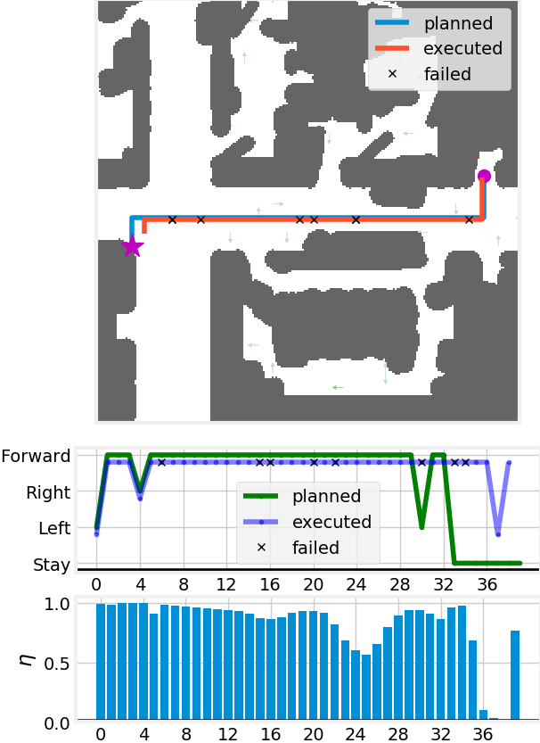
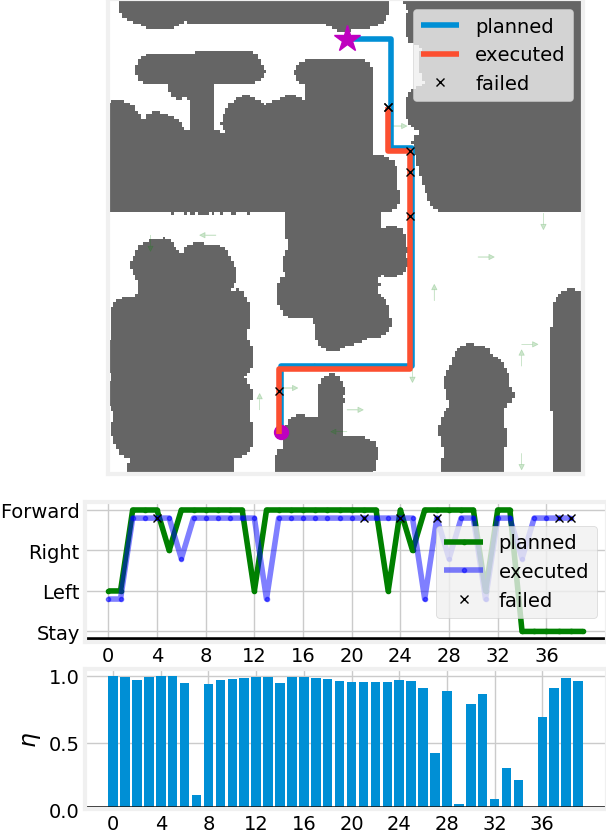
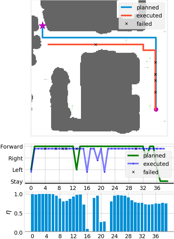
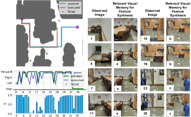
When we vary the number of visual memories given, performance gracefully degrades. In the extreme case, when no visual memories on the planned path are available (denoted ‘40 from env’), our method still outperforms the no visual memory baseline. We also present the distribution of the final distance to goal over different trajectories in Figure 5 (far right) for a much harder test case of following longer trajectories (goal between 32 and 36 time steps away). We notice consistent improvements over open loop execution, as well as, learned closed loop policy. Figure 8 shows some policy executions, policy execution videos are available on the project website.
Full System Evaluation. We also evaluate the performance of the full system in Table 2 in the most challenging setting where the agent is given 40 reference images from the environment, and it has to get to a specified goal location (sampled to be between 16 and 18 steps away), under noisy actuation. We use the joint mapper and planner to compute a plan, that is executed by the learned closed-loop controller. Planning succeeds in 70% cases, open loop execution of these plans succeeds in 20% cases, and our learned plan execution with visual memories succeeds about 27% of the time.
Discussion. This work presents some steps towards learned mapping and landmark based representations for visual navigation. Future work should study more intimate interaction between mapping and landmark systems where path planning can itself be guided by distinctiveness of landmarks along the way, study the problem in continuous action spaces and conduct experiments on real robots.
Acknowledgements: This work was supported in part by Intel/NSF VEC award IIS-1539099, and the Google Fellowship to Saurabh Gupta.
References
- [1] Matterport. https://matterport.com/.
- [2] I. Armeni, O. Sener, A. R. Zamir, H. Jiang, I. Brilakis, M. Fischer, and S. Savarese. 3D semantic parsing of large-scale indoor spaces. In CVPR, 2016.
- [3] B. Axelrod, L. P. Kaelbling, and T. Lozano-Pérez. Provably safe robot navigation with obstacle uncertainty. In RSS, 2017.
- [4] S. Brahmbhatt and J. Hays. Deepnav: Learning to navigate large cities. In CVPR, 2017.
- [5] J. Canny. The complexity of robot motion planning. MIT press, 1988.
- [6] S. Daftry, J. A. Bagnell, and M. Hebert. Learning transferable policies for monocular reactive mav control. In ISER, 2016.
- [7] A. J. Davison and D. W. Murray. Mobile robot localisation using active vision. In ECCV, 1998.
- [8] A. Doucet, N. De Freitas, K. Murphy, and S. Russell. Rao-blackwellised particle filtering for dynamic bayesian networks. In UAI, 2000.
- [9] J. Engel, T. Schöps, and D. Cremers. LSD-SLAM: Large-scale direct monocular SLAM. In ECCV, 2014.
- [10] J. Fuentes-Pacheco, J. Ruiz-Ascencio, and J. M. Rendón-Mancha. Visual simultaneous localization and mapping: a survey. Artificial Intelligence Review, 2015.
- [11] A. Giusti, J. Guzzi, D. C. Cireşan, F.-L. He, J. P. Rodríguez, F. Fontana, M. Faessler, C. Forster, J. Schmidhuber, G. Di Caro, et al. A machine learning approach to visual perception of forest trails for mobile robots. RAL, 2016.
- [12] S. Gupta, J. Davidson, S. Levine, R. Sukthankar, and J. Malik. Cognitive mapping and planning for visual navigation. In CVPR, 2017.
- [13] S. Izadi, D. Kim, O. Hilliges, D. Molyneaux, R. Newcombe, P. Kohli, J. Shotton, S. Hodges, D. Freeman, A. Davison, and A. Fitzgibbon. KinectFusion: real-time 3D reconstruction and interaction using a moving depth camera. UIST, 2011.
- [14] M. Jaderberg, K. Simonyan, A. Zisserman, et al. Spatial transformer networks. In NIPS, 2015.
- [15] G. Kahn, A. Villaflor, B. Ding, P. Abbeel, and S. Levine. Self-supervised deep reinforcement learning with generalized computation graphs for robot navigation. arXiv preprint arXiv:1709.10489, 2017.
- [16] L. E. Kavraki, P. Svestka, J.-C. Latombe, and M. H. Overmars. Probabilistic roadmaps for path planning in high-dimensional configuration spaces. RA, 1996.
- [17] A. Khan, C. Zhang, N. Atanasov, K. Karydis, V. Kumar, and D. D. Lee. Memory augmented control networks. arXiv preprint arXiv:1709.05706, 2017.
- [18] D. Kingma and J. Ba. Adam: A method for stochastic optimization. arXiv preprint arXiv:1412.6980, 2014.
- [19] G. Klein and D. Murray. Parallel tracking and mapping for small AR workspaces. In ISMAR, 2007.
- [20] K. Konolige, J. Bowman, J. Chen, P. Mihelich, M. Calonder, V. Lepetit, and P. Fua. View-based maps. IJRR, 2010.
- [21] S. M. Lavalle and J. J. Kuffner Jr. Rapidly-exploring random trees: Progress and prospects. In Algorithmic and Computational Robotics: New Directions, 2000.
- [22] S. Levine, C. Finn, T. Darrell, and P. Abbeel. End-to-end training of deep visuomotor policies. JMLR, 2016.
- [23] P. Mirowski, R. Pascanu, F. Viola, H. Soyer, A. Ballard, A. Banino, M. Denil, R. Goroshin, L. Sifre, K. Kavukcuoglu, et al. Learning to navigate in complex environments. In ICLR, 2017.
- [24] D. Nistér, O. Naroditsky, and J. Bergen. Visual odometry. In CVPR, 2004.
- [25] E. Parisotto and R. Salakhutdinov. Neural map: Structured memory for deep reinforcement learning. arXiv preprint arXiv:1702.08360, 2017.
- [26] D. A. Pomerleau. Alvinn: An autonomous land vehicle in a neural network. In NIPS, 1989.
- [27] S. Ross, G. J. Gordon, and D. Bagnell. A reduction of imitation learning and structured prediction to no-regret online learning. In AISTATS, 2011.
- [28] F. Sadeghi and S. Levine. (CAD)2RL: Real singel-image flight without a singel real image. In RSS, 2017.
- [29] S. Schaal. Learning from demonstration. In NIPS, 1997.
- [30] B. Siciliano and O. Khatib. Springer handbook of robotics. Springer, 2016.
- [31] A. Tamar, S. Levine, and P. Abbeel. Value iteration networks. In NIPS, 2016.
- [32] S. Thrun, W. Burgard, and D. Fox. Probabilistic robotics. MIT press, 2005.
- [33] E. C. Tolman. Cognitive maps in rats and men. Psychological review, 1948.
- [34] J. M. Wiener, S. J. Büchner, and C. Hölscher. Taxonomy of human wayfinding tasks: A knowledge-based approach. Spatial Cognition & Computation, 9(2):152–165, 2009.
- [35] J. Zhang, L. Tai, J. Boedecker, W. Burgard, and M. Liu. Neural slam. arXiv preprint arXiv:1706.09520, 2017.
- [36] T. Zhou, M. Brown, N. Snavely, and D. G. Lowe. Unsupervised learning of depth and ego-motion from video. In CVPR, 2017.
- [37] Y. Zhu, R. Mottaghi, E. Kolve, J. J. Lim, A. Gupta, L. Fei-Fei, and A. Farhadi. Target-driven visual navigation in indoor scenes using deep reinforcement learning. In ICRA, 2017.