Memory-induced mechanism for self-sustaining activity in networks

Abstract

We study a mechanism of activity sustaining on networks inspired by a well-known model of neuronal dynamics. Our primary focus is the emergence of self-sustaining collective activity patterns, where no single node can stay active by itself, but the activity provided initially is sustained within the collective of interacting agents. In contrast to existing models of self-sustaining activity that are caused by (long) loops present in the network, here we focus on tree–like structures and examine activation mechanisms that are due to temporal memory of the nodes. This approach is motivated by applications in social media, where long network loops are rare or absent. Our results suggest that under a weak behavioral noise, the nodes robustly split into several clusters, with partial synchronization of nodes within each cluster. We also study the randomly-weighted version of the models where the nodes are allowed to change their connection strength (this can model attention redistribution), and show that it does facilitate the self-sustained activity.

I Introduction

The emergence of online social networking and microblogging sites has facilitated novel channels of communication that did not exist under the traditional centralized dissemination model lazar . Online platforms such as Twitter or Facebook enable users to produce content and distribute it through social ties. This process is often modeled via threshold elements, where a node is affected, or activated, whenever the influence of its local environment exceeds a certain threshold. The affected node can then propagate the influence further, probably causing a global activation cascade throughout the whole system watts ; dodds_watts ; galstyan ; gleeson . Studies of such cascades and related dynamic processes on networks have attracted significant attention; see porter2014 ; barrat for recent surveys.

Threshold models have a long history in quantitative sociology, and different variants have been used for describing weak ties weak_ties , social impact granovetter ; latane , and economic activity morris ; durlauf ; stauffer ; econo ; cortes . Another line of research where threshold models are prevalent is neuronal systems peto ; arbib ; stro ; integrate_fire . Indeed, several scholars have noticed certain analogies between social and neuronal systems klopf ; shvyrkov ; nowak ; vidal ; larson . In particular, both social agents and neurons can be viewed as information processing units that gather information from their local neighborhood and act on that information (firing in the case of neurons, posting in the case of social media users). Furthermore, the electrical potential of the neuron can be reinterpreted as an accumulated “information” of the agent. Those analogies were exploited in peto , where conditional reflexes of a single (social) agent were described via a neuronal model.

A popular approach for describing neuronal dynamics is the so-called integrate-and-fire (IF) family of models stro ; integrate_fire , which emerged from the first formalization of neuronal networks proposed by McCulloch and Pitts peto . The IF model was used to examine the conditions under which certain network structures exhibit self-sustained dynamics due to small-world effects roxin ; kaski ; qian ; see also bassett ; davidsen in this context. More recently, the authors of arenas introduced a strongly driven, perfect-memory integrate-and-fire neuronal model for describing the collective dynamics of social networks. The model overcomes one of the main limitations of the cascade approaches (absence of feedback, i.e., each node is active only once) and is applicable to the quantitative description of Twitter data arenas .

In this paper we formulate a simple IF-based model to study mechanisms of collectively sustained activity patterns in networks. Note that we differentiate between activity cascades—activity propagating through the whole system at least once—and the collective activity sustaining, where an agent cannot activate in isolation, but a collective of agents on a network does keep (possibly locally) an initial activity over a sufficiently long time period.

There is a large body of work on collective activity patterns in neuronal systems E-Y ; abbott ; schuster ; anni ; mcgraw ; chin . This activity relates to proactive functions of the brain, e.g., attention and memory fries ; pipa . The main mechanism for self-sustaining collective activity in such systems is based on the existence of cycles in networks, which effectively serve as feedback loops arbib ; mikhailov . Such cycles, also called reverberators, are abundant even in random networks anni ; mcgraw ; chin . Recent research has focused on understanding how the loops contribute to sustained activity and how their embedding in a network affects the activity patterns anni ; mcgraw ; chin . Besides neuronal networks, self-sustained collective oscillations are observed in other systems others .

Here we are interested in alternative mechanisms for collective activity, which do not rely on the existence of long cycles. In particular, we are motivated by recent observations that the effective networks in social media might not necessarily have long loops. For instance, it has been established that the functional networks inferred using the activity traces of the users are tree-like, with relatively short loops; see Sec. II.5 for details. Thus, it is important to have a different mechanism of self-sustaining cascades that does not involve long feedback loops.

The proposed mechanism of self-sustaining activity patterns is based on temporal memory of an individual agent. Namely, we show that there is a parameter range of memory and inter-agent coupling that allows self-sustaining collective activity patterns. The underlying reason for emergence of this regime is the fragmentation of the network into (partially synchronized) clusters. Furthermore, it is shown that under a weak (behavioral) noise, this fragmentation is robust with respect to details of the activation process, number of nodes, initial conditions, the noise model, etc.

We also study the activation dynamic on randomly weighted networks, where the weights can be interpreted as attention the nodes pay to their neighbors. Our numerical results indicate that the introduction of random weights does facilitate activity sustaining, sometimes even violating intuitively obvious bounds.

The remainder of this paper is organized as follows. We introduce the model in Section II. Section III outlines the memory-less situation, while in Section IV we deduce the implications of an agent’s memory for self-sustaining collective activity. In Section V we study the effect of weak noise. Section VI shows how limitations on the agent’s attention can be described via a (randomly) weighted network. We conclude by discussing our main results in Section VII.

II The model

II.1 Neurons versus agents

Before introducing our model, let us recall some essential facts about information processing by neurons. A neuron collects signals from its environment and from other neurons via dendrites (in-going channels) peto . These signals build up its electrical potential. Once this potential is larger than a certain threshold, the neuron fires (generates a signal) via its single out-going channel, axon . The signal is received by all neurons that are connected (via their dendrites) to the axon. After the neuron fires, the potential nullifies. It can accumulate again after some null period peto . Certain neurons do have an internal ability to generate signals even in isolation from other neurons peto .

To establish the analogy with a social system, we assume that the $i$’th agent in our social system is characterized by informational potential $w_{i}$, which can be modified due to content that the agent receives from his neighbors. We assume that whenever $w_{i}$ overcomes a certain threshold $u_{i}$, the agent displays the generated content (fires). Immediately after that event, the information potential nullifies, and then starts to accumulate again.

II.2 Basic equations

For each agent $i$ ($i=1,...,N$) we introduce a variable $m_{i}(t)$ that can assume two values, $0$ (passive with respect to content generation) and $1$ (content generating) at discrete time $t$. The state dynamics are described as

$$m_{i}(t) = \vartheta[\,w_{i}(t)-u_{i}\,],$$ (1)

$$w_{i}(t+1) = [1-m_{i}(t)]\times$$ (2)

$$[\,(1-\kappa_{i})w_{i}(t)+r_{i}+{\sum}_{j}q_{ij}m_{j}(t)\,],~{}~{}$$

where $w_{i}(t)\geq 0$ is the information potential accumulated by the agent $i$ till time $t$, ${\sum}_{j}q_{ij}m_{j}(k)$ is the cumulative influence from other agents (we assume $q_{ii}=0$), and $\vartheta(x)$ is the step function:

$$\vartheta(x<0)=0,~{}~{}\vartheta(x\geq 0)=1.$$ (3)

In Eqs. (1, 2), $u_{i}$ is the threshold, $r_{i}$ is the external rate of potential generation, while $1\geq\kappa_{i}\geq 0$ can be interpreted as the rate of memory decay (or forgetting). The prefactor $[1-m_{i}(t)]$ in front of Eq. (2) ensures that the information potential of an agent nullifies after displaying content.

The influence $q_{ij}m_{j}(t)$ of the agent $j$ on the potential $w_{i}$ of $i$ is non-zero provided that $j$ is in its content-displaying state, $m_{j}(t)=1$. Depending on the sign of $q_{ij}$, this influence can encourage or discourage $i$ in expressing itself. Here we assume that demotivating agents are absent, so we have

$$q_{ij}\geq 0,~{}~{}~{}{\rm and}~{}~{}~{}w_{i}\geq 0.$$ (4)

In the memoryless limit $\kappa=1$, Eqs. (1, 2) relate to the deterministic neuronal dynamics model introduced by McCulloch and Pitts peto . The original McCulloch-Pitts model also included strong inhibition that is absent in the present model. In the continuous time-limit, Eqs. (1, 2) reduce to the integrate and fire model stro ; integrate_fire .

II.3 Isolated agent

For $q_{ij}=0$, Eq. (2) reduces to

$$w(0)=0,\qquad w(t)=\frac{r}{\kappa}[1-(1-\kappa)^{t}],~{}~{}t=1,2,...$$ (5)

Thus, $w(t)$ monotonically increases from $0$ to $\frac{r}{\kappa}$: if $u<\frac{r}{\kappa}$, the agent fires with a period determined from Eq. (5); otherwise it never fires.

II.4 Behavioral noise

The deterministic firing rule given by Eq. (1) should be modified to account for agents with behavioral noise. Specifically, we want to make it possible for an agent to fire (not to fire) even for sub-threshold (super-threshold) values of the potential. The noise will be implemented by assuming that the threshold $u_{i}+v_{i}(t)$ has (besides the deterministic component $u_{i}$) a random component $v_{i}(t)$. These quantities are independently distributed over $t$ and $i$. We shall employ two models for the behavior of $v_{i}(t)$.

Within the first model, $v_{i}(t)$ is a trichotomic random variable, which takes values $v_{i}(t)=\pm V$ with probabilities $\frac{\eta}{2}$ each, and $v_{i}(t)=0$ (no noise) with probability $1-\eta$. In this representation, $\eta$ describes the magnitude of the noise. We assume that $V$ is a large number, so that with probability $\eta$, the agent ignores $w_{i}$ and activates (or does not activate) randomly. Thus, instead of Eq. (1), we now have

$$m_{i}(t)=\vartheta[\,\phi_{i}(t)(\,w_{i}(t)-u_{i}\,)\,].$$ (6)

In Eq. (1), $\phi_{i}$ are independent (over $i$ and over $t$) random variables that assume values $\pm 1$ with probabilities

$${\rm Pr}[\phi_{i}=1]=1-\eta,\qquad{\rm Pr}[\phi_{i}=-1]=\eta.$$ (7)

Our second model, which has wide applicability in neural network literature peto , amounts to replacing the step function by a sigmoid function. Instead of Eq. (1), we now have

$$m_{i}(t) = 1~{}~{}~{}{\rm with\,probability}~{}~{}~{}\frac{e^{(w_{i}(t)-u_{i}\,)/\theta}}{1+e^{(w_{i}(t)-u_{i}\,)/\theta}},$$ (8)

$$= 0~{}~{}~{}{\rm with\,probability}~{}~{}~{}\frac{1}{1+e^{(w_{i}(t)-u_{i}\,)/\theta}},$$ (9)

where $\theta\geq 0$ has the (formal) meaning of temperature, so that the noiseless model is recovered when $\theta\to 0$.

In this paper we limit ourselves to the weak-noise limit ($\eta$ and $\theta$ are small). As illustrated below, both models (6, 8) lead to similar predictions.

II.5 Choice of the network

To proceed further, we have to specify the network structure on which the activation process unfolds. For social media platforms such as Twitter, it seems straightforward to identify the network structure using the declared list of friends and followers. This choice, however, does not necessarily reflect the true interactions that are responsible for the activity spreading huberman . Indeed, there is accumulating evidence that a considerable part of links in Twitter’s follower/friendship network are meaningless, in the sense that they do not necessarily participate in information diffusion. Instead, one has to pay attention to functional links, which are based on the observed activity patterns of the users. One possible way for inferring such functional networks based on transfer entropy (or information transfer) was suggested in Ref. www2012 . As compared to formally declared networks, the ones based on the activity dynamics have fewer loops huberman ; www2012 .

Here is an example that illustrates this point and motivates the introduction of a model network below. A dataset was collected from Spanish Twitter, which contains 0.5 million Spanish messages publicly exchanged through this platform from the 25th of April to the 25th of May, 2011. This dataset was already studied in arenas . We constructed the user-activity network via the transfer-entropy method www2012 ; wsdm2013 , and found that over 99 % of all nodes (users) do have loops attached to them; among those loops 84 % have length 2 (reciprocity), while other loops have length 3; loops of length $\geq$4 are either negligible or absent.

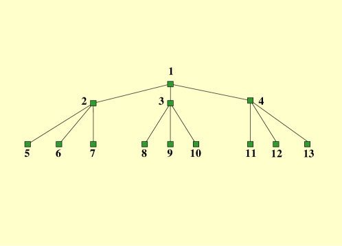
Hence, we need a network model that is (nearly) symmetric, does not contain loops of length 4 and larger and allows a well-controlled introduction of triangles (loops of length 3). As the basic model, here we focus on the (undirected) Cayley tree: one node is taken as the root (zeroth generation) and then $K$ symmetric links are drawn from it (nodes of the first generation); see Fig. 1. In subsequent generations, each node of the previous generation produces $K$ symmetric links. Nodes of the last generation belong to the periphery, and each of them has only one connection. All other nodes belong to the core. The root is connected with $K$ nodes, while all other nodes in the core have $K+1$ connections. If the Cayley tree has $p$ generations, then the overall number of nodes is

$$N=(K^{p+1}-1)/(K-1)=gK+1,$$ (10)

where $g$ is the number of nodes in the core.

Obviously, a Cayley tree has no loops. In our analysis, we will also examine the effect of short loops via addition of a fixed amount of triangles, generated by randomly linking pairs of nodes from the same generation. A similar procedure of studying the influence of triangles (or other mesoscopic network structures) is frequently applied in literature peron . As we show below, these triangles do not lead to quantitative changes, at least for the scenarios examined here; see peron for related results.

In addition to being loop-free, the Cayley tree has another characteristic that makes it a suitable choice for the present study. Specifically, one of the main mesoscopic motifs observed in real-world complex networks is the core-periphery structure, where some of the nodes are well interconnected (core), while sparsely connected periphery is around the core; see freeman ; everett ; bocca ; puck for reviews. The Cayley tree is one of the simplest network models that exhibits features consistent with the definition of the core-periphery structure freeman : (i) the core is more connected than the periphery; (ii) core nodes are located on geodesics connecting many pairs of nodes (large betweenness degree); (iii) core nodes are minimally distant from (possibly many) other nodes. As we show below, the identification of the core-periphery structure for the Cayley tree is reflected in the dynamics of the model defined on it.

III Clustering and synchronization due to strong coupling

In Eqs. (1, 2) we assume that all agents are equivalent and that the network is not weighted:

$$r=r_{i},~{}~{}~{}~{}u=u_{i},~{}~{}~{}~{}\kappa=\kappa_{i},~{}~{}~{}~{}q_{ij}=q.$$ (11)

Note that for

$$q>u-r>0,$$ (12)

activation of one agent is sufficient for exciting his neighbors. This is not a realistic condition. Below we will almost always assume that $q<u-r$. However, let us first discuss what happens when Eq. (12) is valid. We can focus on the memoryless situation $\kappa=1$, since under the condition Eq.(12), the memory is not relevant. We stress that $u>r$ in Eq. (12) means that that no agent is able to activate spontaneously by itself (i.e., for $q=0$); cf. Eq. (5).

Our numerical results are summarized as follows. Provided that there is at least one active agent ($m_{i}(0)=1$) initially, after a few time-steps the system converges to a fully synchronized state, where it separates into two clusters: the first cluster mainly includes the core, while the second cluster mainly includes periphery. If the first cluster is active, then the second one is passive, and vice versa. All agents have nearly the same firing frequency that is close to its maximal value of $0.5$. Finally, this scenario exists for any $K\geq 1$.

Thus, the clusters alternate their active states, with one cluster collectively exciting the other. Note that neither of those clusters can sustain activity by itself, because after each activation, the potential for all the nodes drops to zero, and no isolated agent can be activated by itself.

If instead of Eq. (12) we set $u>r+q$ (but $r<u$ and $\kappa=1$), then the system converges to a trivial passive fixed point for all initial states, where any initial activity dies out after a few time-steps. This behavior crucially depends on the fact that the Cayley tree does not have sufficiently long loops .

The above results remain qualitatively valid after adding (randomly) up to $\sim N/K\approx g$ triangles. The same threshold (12) holds in this case.

IV Collective dynamics driven by memory

IV.1 Thresholds of self-sustaining activity

If the coupling is not strong, $0<q<u-r$, our numerical results suggest that there is a self-sustaining collective activity regime, which exists under the following conditions:
$\imath)$ There should be sufficiently many neighbors:

$$K\geq 2.$$ (13)

$\imath\imath)$ The memory should be non-zero, $\kappa<1$, but still small enough so that no agent can fire in isolation [see Eq. (5), and note that conditions of Eq.(11) hold]:

$$u>r/\kappa.$$ (14)

Without loss of generality, below we set

$$u_{i}=1,$$ (15)

Note that $u=u_{i}$ can be adjusted by varying the parameters $1-\kappa$, $r$ and $q$; see Eqs. (1, 2).

The simulations of the model reveal that the collective activity pattern in this regime—and its very existence—depend on initial conditions $\{w_{i}(0)\}_{i=1}^{N}$ of Eqs. (1, 2), i.e., the choice of initially active nodes. To describe this dependence, we assume that in the initial vector $\{w_{i}(0)\}_{i=1}^{N}$ each $w_{i}(0)$ is generated randomly and homogeneously in the interval.

$$[0,b],~{}~{}~{}2>b>1.$$ (16)

For $N\gg 1$, Eqs. (15, 16) imply that $\simeq(b-1)N/b$ agents are active in the initial state (for them $m_{i}(0)=1$).

Numerical results show that there exists an upper threshold ${\cal Q}^{+}<1$, such that for $q>{\cal Q}^{+}$ (and all other parameters being fixed), the collective activity is sustained in time for (almost) all realizations of the random initial state:

$$q>{\cal Q}^{+}\Longrightarrow m(t)\equiv\frac{1}{N}\sum_{k=1}^{N}m_{i}(t)\not=0~{}~{}{\rm for}~{}~{}t>0.$$ (17)

Likewise, there is a lower threshold ${\cal Q}^{-}<{\cal Q}^{+}$ such that for $q<{\cal Q}^{-}$ the activity decays to zero in a finite time $T$ for (almost) all initial states:

$$q<{\cal Q}^{-}\Longrightarrow m(t)=0~{}~{}{\rm for}~{}~{}t>T.$$ (18)

In the range ${\cal Q}^{-}\leq q\leq{\cal Q}^{+}$, whether or not the initial activity will be sustained depends on the realization of the random initial state $\{w_{i}(0)\}_{i=1}^{N}$; see Figs. 2, 3, 4 and 5.

The thresholds ${\cal Q}^{+}$ and ${\cal Q}^{-}$ depend on all the model parameters: $\kappa$, $r$, $b$, $K$ and $N$. They are decreasing functions of $N$, provided $N$ is sufficiently large; see Table I. They are also increasing functions of $\kappa$ and saturate at ${\cal Q}^{+}={\cal Q}^{-}=u=1$ for $\kappa=1$ (no memory); see Section III. The difference ${\cal Q}^{+}-{\cal Q}^{-}$ is small, but it persists for large values of $N$; see Table I.

Consider a pertinent case where only one agent is active initially. We find that in this case the thresholds are still non-trivial; e.g., for parameters of Fig. 5 we obtain ${\cal Q}^{+}[b\to 1+]=0.524$, while ${\cal Q}^{+}[b=1.8]=0.358$. Also, for this example of $b\to 1$, the collective activity $m(t)=\frac{1}{N}\sum_{k=1}^{N}m_{i}(t)$ reaches $0.1$, when starting from $1/N=1.66\times 10^{-4}$ at $t=0$.

Note that there is a simple lower bound on ${\cal Q}^{-}$:

$${\cal Q}^{-}>\frac{1-r}{K}.$$ (19)

To understand the origin of this bound, recall that owing to Eq. (14), the agents cannot activate spontaneously. If $q<\frac{1-r}{K}$, then even all stimulating connections (acting together) cannot activate the agent, so that no initial activity can be sustained.

Finally, note that for cascading processes there is typically a single threshold that depends on network structure porter2014 ; barrat , even if one takes into account possible feedback effects in the activation dynamics arenas .

IV.2 Clustering and synchronization

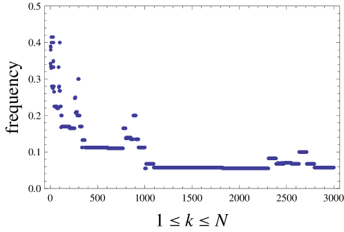
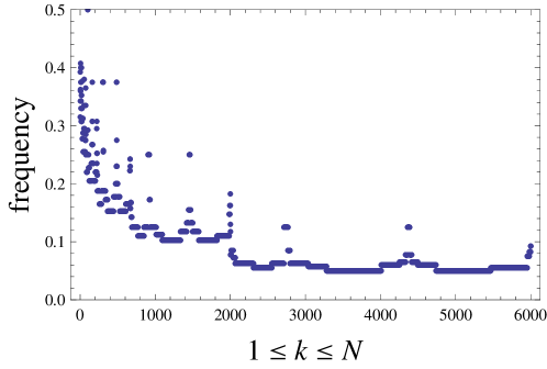
Our analysis suggests that the activity sustaining occurs via separation of the network into clusters (groups) of neighboring agents, having the same firing frequency; see Figs. 2, 3 and 4 (note that certain nodes do not belong to any cluster). The number of clusters and their distribution depend on the realization of the (random) initial state; cf. Figs. 2, 3 with Figs. 4. Furthermore, this dependence persists in the long time limit, suggesting that the long-term behavior cannot be adequately described by mean-field analysis that involves only few parameters. Concrete scenarios of clusterization can differ from each other widely; e.g., there is a scenario (related to specific initial states) where the distribution of clusters is very regular, ranging from the core to the periphery of the Cayley tree; see Figs. 2.

Within each cluster $C$ the firing frequency of agents is synchronized; i.e., the collective intra-cluster activity

$$m_{C}(t)=\frac{1}{N_{C}}\sum_{i\in{C}}m_{i}(t),$$ (20)

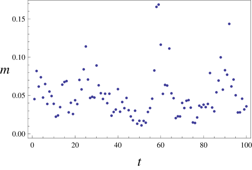
where $N_{\rm C}$ is the number of agents in the cluster ${C}$ has a regular time-dependence; see Figs. 3, 3, and 4. This dependence is displayed via few horizontal lines along which $m_{C}(t)$ changes.

The distribution of clusters shows two common features: there is a cluster that involves the major part of the periphery and a smaller cluster that is located inside of the core, close to the core-periphery boundary; see Figs. 2, 4. For all realizations of the initial state, where the activity is sustained over a long time, there is a clear transition between the core and the periphery.

There are two well-separated time-scales here: after the first time-scale ($\sim 50-100$ time steps for parameters of Figs. 2, 3 and 4) the structure of clusters is visible, but the intra-cluster activity is not synchronized; i.e., $m_{\cal C}(t)$ looks like a random function of time. The achievement of intra-cluster synchronization takes a much longer time, e.g., $\sim 10^{3}$ time-steps for parameters of Figs. 2, 3 and 4.

Figs. 5 and 5 show that after adding (randomly distributed) triangles (loops of length 3), the distribution of firing frequencies becomes smeared, and the separation into well-defined clusters is less visible. There is also a visible maximum of the frequency distribution at the boundary between the core and periphery (i.e., at $k\sim g$). Note that adding triangles does not change the thresholds ${\cal Q}^{+}$ and ${\cal Q}^{-}$ if the number of triangles is not large (smaller than 30 - 40 % of nodes); cf. Section II.5.

Table 1: Activity sustaining thresholds ${\cal Q}^{+}$, ${\cal Q}^{-}$ versus the overall number $N$ of agents for $u=1$, $r=0.1$, $\kappa=0.101$, $K=3$ and $b=1.8$. Due to numerical errors, the numeric results given below overestimate (underestimate) the value of ${\cal Q}^{+}$ (${\cal Q}^{-}$).

$N$	${\cal Q}^{+}$	${\cal Q}^{-}$
$1.5\times 10^{3}$	0.404	0.356
$3\times 10^{3}$	0.365	0.354
$6\times 10^{3}$	0.358	0.333
$1.5\times 10^{4}$	$0.358$	0.305

To summarize this section, the model studied here has revealed two novel aspects of collective dynamics on networks. First, it shows that agent memory can facilitate collective activity sustaining (via clustering and synchronization), even on networks without long loops. And second, the model has two relevant (upper and lower) thresholds ${\cal Q}^{+}$ and ${\cal Q}^{-}$, so that in-between these thresholds, the dynamics are very complex and sensitive to initial conditions. Further generalizations of this model that include effects of external noise and network weighting are studied below.

IV.3 Relation to prior work

Synchronization is well-known in neuroscience, because it relates to the normal activity pattern of brain neurons; see peto ; mikhailov ; mimi for reviews. It is seen on EEG measurement, where macroscopic (many-neuron) activity is recorded and temporal correlations are found between, e.g., the left and right hemispheres of the brain peto ; mikhailov ; mimi . Synchronized states are relevant for the brain functioning; they relate to consciousness, attention, memory, and also to pathologies (e.g., epilepsy).

For the fully connected—all neurons couple with each other with the same weight—integrate and fire model (1, 2) the fully synchronized state was studied in stro . The existence of a few-cluster synchronized state was predicted in abbott ; schuster , though the existence of two different thresholds ${\cal Q}^{+}$ and ${\cal Q}^{-}$ were not seen, and the relation between memory, loop-structure of the network and the activity sustaining was not recognized.

The existence of non-ergodic (initial state-dependent) fragmentation into clusters is well-known for coupled chaotic maps kaneko ; crisanti ; manrubia_non_ergo ; mikhailov ; mimi ; gade . This many-attractor situation can be considered as a model for neuronal memory peto . However, the existing scenarios of clusterization are based on a sufficiently strong inter-neuron coupling on a network that admits long loops; cf. also roxin ; kaski ; qian . Ref. gade studied a specific model of coupled maps on the Cayley tree, but only two relatively simple synchronization scenarios were uncovered.

Thus, two novelties of our results are that we single out a specific mechanism for generating clustering and synchronization (memory on a network with long loops), and we show that these phenomena (apart of various details) relate to two different thresholds ${\cal Q}^{+}$ and ${\cal Q}^{-}$. Further generalizations of this model that include effects of external noise and network weighting are studied below.

V Noise-driven clusterization

We now consider the model Eqs. (1, 2) under the behavioral noise, defined by Eqs. (6, 7). As in the noiseless case, we assume that both Eq. (13) and Eq. (14) hold, e.g., each node has sufficiently many neighbors, each node has sufficiently strong memory, but without the possibility of activating spontaneously.

In addition, we will also assume that the following conditions hold:

$\imath)$ Weak noise: $\eta\ll 1$. Thus an isolated agent (for $q=0$) will fire randomly with the average activity $\eta$.

$\imath\imath)$ Sub-threshold coupling: $0<q<{\cal Q}^{-}$, i.e., no activity is sustained without the noise; see Eqs. (17, 18).

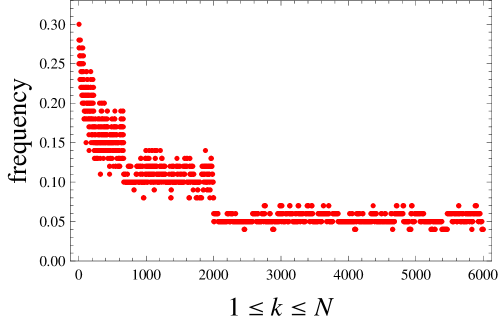
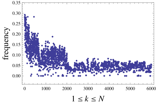
Under the above conditions, the dynamics lead to the fragmentation of the network into several clusters; see Fig. 6. A cluster is a set of neighbor agents with approximately identical firing frequencies; see Fig. 6. The firing frequency is defined as the number of firings in an interval

$$[\tau_{0},\tau_{0}+\tau]$$ (21)

divided over the interval length $\tau$. Here $\tau_{0}$ has to be sufficiently large for the system to become independent from the initial state $\{w_{i}(0)\}_{i=1}^{N}$. If $\tau$ is sufficiently large as well, the distribution of frequencies does not change upon its further increase; see Fig. 6.

The overall number of clusters is never larger than 4— see Fig. 6, where it equals 4. The number of clusters decreases for larger $q$, because clusters located in the core tend to merge with each other: for $q$ close to (but smaller than) $u=1$, there remain only 2 clusters—those involving (respectively) core and periphery. The distribution of clusters does not depend on the initial conditions, i.e. no special conditions such as one specified by Eq. (16) are needed. This is in stark contrast with the noiseless situation, where the number and structure of clusters are sensitive to initial conditions.

The smallest cluster includes the root of the Cayley tree, and has the largest firing frequency. The largest cluster includes the whole periphery; here the (average) firing frequency is the smallest one, but it is still clearly larger than the noise magnitude $\eta$.

Additional structure of clusters is observed by analyzing the short-time activity, i.e., when $\tau$ in Eq. (21) is not very large; see Fig. 6. Each cluster consists of sub-clusters that also have (nearly) the same firing frequency. Comparing Figs. 6 and 6 we see that there are “boundary” agents: within the short-time [long-time] activity they do not [do] belong to a definite cluster; cf. Fig. 6 with Fig. 6.

The above clusterization disappears under sufficiently strong noise, which makes all the nodes equivalent. Fig. 6 shows that the influence of weak noise is non-additive: the resulting agent activity (even in the periphery) is larger than the noise magnitude $\eta$. The fragmentation into clusters and the non-additivity disappear if the magnitude of memory decreases; e.g., for parameters of Fig. 6 (where $\kappa=0.101$) both effects disappear for $\kappa=0.2$.

Note that the correspondence between noisy and noiseless results is there for limited times and for $\eta$ being sufficiently smaller than $0.01$; see Fig. 7 for an example.

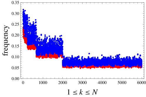
The results above were obtained under the noise model (6, 7). Similar results are obtained for the model (8); cf. Fig. 6 with 7. The main difference between the two models (provided that we identify them via $\eta=\theta$) is that for Eq. (8) the spread around the average frequency is smaller. This is expected, since Eqs. (6, 7) refer to a noise that can assume large values.

Finally, we note that introducing triangles does not alter the cluster structure, but can increase the activity—sometimes sizeably; see Fig. 8.

VI Randomly weighted network

VI.1 Weighting and attention distribution

So far, we assumed that each agent stimulates its neighbors in exactly the same way, so that the link wights $q_{ij}$ do not depend on $j$, and each connection gives the same contribution to the information potential $w_{i}$ of the $i$’th agent; cf. Eq. (11). This is clearly an oversimplification, as different connections are usually prioritized differently. This prioritization can be related to the attention an agent pays to his neighborsv_at ; hu_at .

Below we extend our model to account for weighted attention mechanims. We consider two different weighting schemes, frozen (or quenched), where the link weights are static random variables, and annealed, where the weights ate frequently resampled from some distribution .

VI.2 Frozen versus annealed random weights

Under this model, the link weights $q_{ij}$-s are frozen (i.e., time-independent) random variables, sampled from some distribution. To account for limited attention of the agents, we require the cumulative weight stimulating each agent to be fixed. Thus, we use the following weighting scheme:

$$q_{ij}=q\phi_{i}\tau_{ij},\qquad\sum_{j=1}^{\phi_{i}}\tau_{ij}=1,$$ (22)

where $\phi_{i}$ is the number of neighbors for agent $i$: $\phi_{1}=K$, $\phi_{1<i\leq g}=K+1$, $\phi_{i>g}=1$; cf. Fig. 1.

Eq. (22) allows a comparison with the non-weighted situation, where $\tau_{ij}=1/\phi_{i}$ for all $i$ and $j$. Generally speaking, we can generate $\tau_{ij}$-s by sampling from any distribution defined over a $\phi_{i}$-dimensional simplex. Here we construct $\tau_{ij}$ by sampling $\phi_{i}$ independent random numbers $n_{ij}$ and then normalizing them malsburg

$$\tau_{ij}=n_{ij}\left/\sum_{l=1}^{\phi_{i}}n_{il}\right..$$ (23)

In the numerical results reported below, we assume that $n_{ij}$ are generated independently and homogeneously in the interval $[0,b^{\prime}]$ with $b^{\prime}=10$. We found that if $b^{\prime}$ is sufficiently larger than $1$, its concrete value is not essential, e.g., $b^{\prime}=10$ and $b^{\prime}=100$ produce nearly identical results.

Our numerical results suggest that the introduction of (frozen) random weights results in modified upper and lower thresholds ${\cal Q}^{+}_{f}$ and ${\cal Q}^{-}_{f}$; cf. Eqs. (17, 18). For $q>{\cal Q}^{+}_{f}$ [$q<{\cal Q}^{-}_{f}$], any initial activity persists [does not persist] in the long-time limit, irrespective of the initial conditions $\{w_{i}(0)\}_{i=1}^{N}$ and the attention distribution $\{\tau_{ij}\}$. For ${\cal Q}^{-}_{f}<q<{\cal Q}^{+}_{f}$, the existence of a long-time activity depends on realizations of $\{\tau_{ij}\}$ and of $\{w_{i}(0)\}_{i=1}^{N}$.

Our analysis yields [cf. Eqs. (17, 18)]

$${\cal Q}^{+}_{f}<{\cal Q}^{+},~{}~{}~{}{\cal Q}^{-}_{f}<{\cal Q}^{-},$$ (24)

which means that introduction of frozen weights facilitates the long-term activity sustaining. Moreover, we find that ${\cal Q}^{-}_{f}$ can be lower than the trivial bound given by Eq. (19), e.g., for parameters of Fig. 10: ${\cal Q}^{-}_{f}=0.265$, whereas (19) gives $0.3$. Recall that Eq. (19) holds strictly only for the non-weighted scenario. Though $q$ in Eq. (19) still characterizes the average magnitude of each connection also in the weighted situation [cf. Eq. (22)], numerical results reported in Figs. 9, 9 and 10 show that Eq. (19) does not extend to this situation (both for frozen and annealed weighting schemes, as seen below) .

Random frozen weights increase activity (as compared to the non-weighted situation), because there are $\tau_{ij}$ which is close to one; hence there are links with the weight close to $Kq$, which is $K$ times larger than for the non-weighted case, where all weights are equal to $q$. Of course, there are also $\tau_{ij}$’s which are close to zero, since both situations have the same average weight per node; see Eq. (22). But the influence of those weak weights on the activity sustaining appears to be weaker.

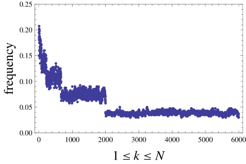
Similar to the non-weighted (and noisy) scenario in Section V, the dynamical system defined on the weighted network factorizes into several clusters, which themselves consist of sub-clusters, as seen by looking at the short-time activity; see Figs. 9 and 9. However, the cluster structure is somewhat different compared to the non-weighted situation. Namely, different clusters can have agents that fire with (approximately) equal frequencies, but different clusters are separated from each other by regions of low (but non-zero) activity. This is especially visible near the threshold ${\cal Q}^{-}_{f}$; see Fig. 10.

For the annealed random situation a new set of random weights is generated independently (and according to Eqs. (22, 23)) at each time-step $t$. The corresponding thresholds ${\cal Q}^{+}_{a}$ and ${\cal Q}^{-}_{a}$ appear to be lower than (respectively) the ${\cal Q}^{+}_{f}$ and ${\cal Q}^{-}_{f}$; cf. Eq. (24). For example, ${\cal Q}^{-}_{f}=0.265$ and ${\cal Q}^{-}_{a}=0.245$ for parameters of Figs. 9 and 9.

As Figs. 11–12 show, the activity pattern in the annealed situation is similar to the noisy, non-weighted situation described in Section V (recall however that the latter does not have sharp thresholds; the activity there decays together with the magnitude of noise). In particular, this similarity concerns the factorization into clusters [cf. Fig. 11 with Fig. 6] and short-term versus long-term activity [cf. Fig. 12 with Fig. 6].

VII Conclusion

We have studied mechanisms for self-sustaining collective activity in networks using an activation model inspired by neuronal dynamics (1, 2). Our specific set-up was motivated by the empirical observation [see Section II.5] that the social networks composed of functional links do not have long loops (involving more then three nodes). As a concrete implementation of this type of network, we focused on the Cayley tree with randomly added triangles, and examine memory-induced mechanisms of sustaining activity patterns on those networks.

We uncovered several scenarios where the network is capable of sustaining collective activity patterns for arbitrarily long times. For the non-weighted Cayley tree (with noiseless agents), we observe a fragmentation of the network into several clusters (see Section IV), so that the activity of the agents within each cluster is synchronized. The clusterization and synchronization proceed along different timescales: the former is (much) quicker than the latter. It is thus possible that at certain observation times, only clustering will be observed.

The collective activity sustaining is observed whenever the inter-agent coupling $q$ is larger than a certain threshold ${\cal Q}^{+}$. Among other parameters, ${\cal Q}^{+}$ depends on the amount of activation provided initially. The structure (and number) of clusters depends not only on this amount, but also on which agents are activated initially. For ${\cal Q}^{-}<q<{\cal Q}^{+}$ (where ${\cal Q}^{-}$ is a lower threshold), the dynamics strongly depend on initial conditions. Thus, this model does show selectivity with respect to initial activation, i.e., some agents play a role of effective activity sustainers. Note that these features of activity sustaining thresholds differ from those of cascade thresholds that depend mostly on the network structure, even if the feedback effects on cascades are accounted for arenas .

The above dependencies on initial conditions are eliminated under the influence of a (behavioral) agent noise; see Section V. Under this noise, the network robustly fragments into few (short-time synchronized) clusters, while the activity sustaining does not have a threshold character. These conclusions do not depend on the model of noise.

We also studied a more realistic situation where the network is randomly weighted, i.e., there is a random distribution of priorities. Our results indicate that the presence of weights does facilitate the activity sustaining, and leads to a different scenario of clusterization, where clusters are (physically) more isolated from each other; see Section VI.

This study was confined to a model-dependent situation; in particular, we worked on the level of the Cayley tree for the network (not a fully realistic functional network), and we did not attempt any direct data-fitting. But the results of this model do suggest several directions for empiric (data-driven) research. To what extent can the activity pattern in real social media be modeled via (partially synchronized) clusters of agents? Do behavioral noise and weighting (attention re-distribution) have to be accounted for explicitly?

We also note that in this study we assumed that all the connections are facilitating; see Eq. (4). It is known that the inhibitory connections do play a crucial role in sustaining and shaping the (biological) neuronal activity peto . As future work, it will be interesting to see the extent to which such inhibitory connections are present in the interactions in social media, and how they affect the collective activity patterns.

Figures

Figure 1: (Color online) The Cayley tree with $K=3$ and two generations. The nodes $5-13$ belong to periphery. The nodes are numbered from the root of the tree, i.e. $k=1$ is the root, $k=g$ is the last node of the core, and $k=N$ is the last node in the periphery; cf. Eq. (10).

Figure 2: (Color online) Firing frequency and activity for agents with memory in the noiseless situation. The agents are numbered as in Fig. 1.
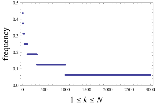
Parameters: $u=1$, $r=0.1$, $\kappa=0.101$ and $q=0.36$. This value of $q$ is between of two thresholds ${\cal Q}^{+}>q>{\cal Q}^{-}$; see Table I. The initial condition was generated with $b=1.8$; see Eq. (16). Parameters of the Cayley tree: $K=3$, $N=3\times 10^{3}+1$ (total number of nodes).
Frequency of each node versus the number of node number. The frequency is defined as the number of firings in the time-interval $[1200,1600]$ divided over the interval length $400$. For this specific realization of the initial state, the cluster structure is very regular.

Figure 3: (Color online) The same parameters as in Fig. 2.
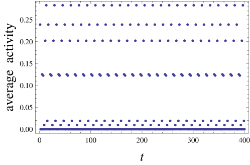
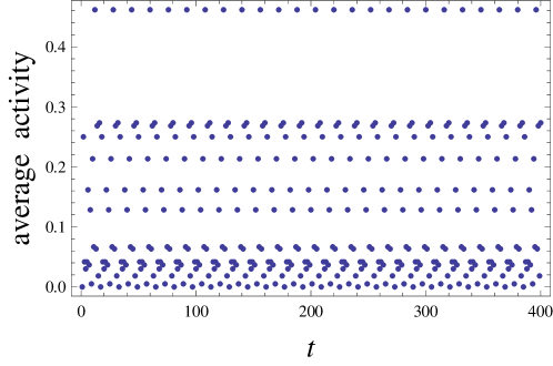
(a) The average activity $m(t)=\frac{1}{2000}\sum_{k=1000}^{3000}m_{k}(t)$ of the peripheric cluster versus time $t+1200$.
(b) The average activity $m(t)=\frac{1}{700}\sum_{k=300}^{1000}m_{k}(t)$ of the outer core cluster versus time $t+1200$.

Figure 4: The same as in Figs. 2, but for another realization of the random initial condition generated with $b=1.8$; see Eq. (16).

Figure 5: (Color Online) Comparison of firing frequencies with and without triangles.
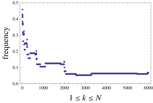
(a) The Cayley tree without triangles: frequency of fairing in the interval $[1200,1600]$ divided over the interval length $400$. The parameters are the same as in Figs. 2, but with $N=6\times 10^{3}+1$.
(b) The same as in (a), but with randomly added 1050 links that define 1050 triangles.

Figure 6: (Color Online) Dynamics under behavioral noise with magnitude $\eta=0.01$; cf. Eqs. (6, 7).
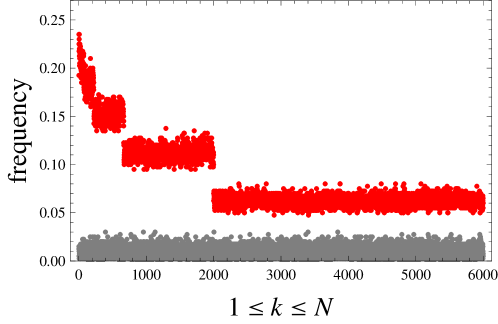
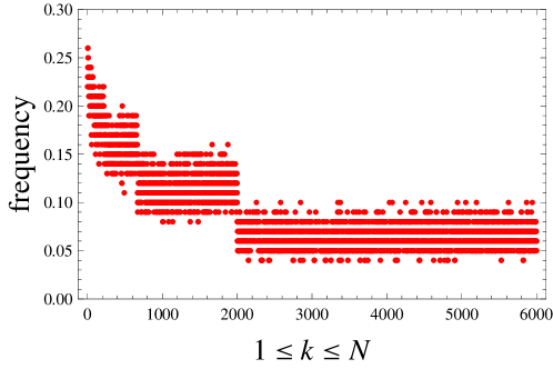
(a) Red points (upper stripes): Frequency of each agent versus the agent number: the number of fairings in the interval $[400,800]$ divided over the interval length $400$ for $u=1$, $r=0.1$, $\kappa=0.101$, $K=3$, $N=6\times 10^{3}+1$ (total number of nodes), $q=0.3$ (subthreshold situation: $q<{\cal Q}^{-}$; see Table I). The initial state is passive: $w_{i}(0)=0$. The core-periphery border is at $k=2000$. The time-average of $m(t)$ equals $0.08$. Gray points (the lowest stripe): the same as for blue points but for $q=0$ (isolated agents). The time-average of $m(t)$ equals to the noise magnitude $0.01$.
(b) The same as in (a), but the firings are counted in the interval $[400,500]$ and are divided over the interval length $100$.

Figure 7: (Color Online) (a) The same as in Fig. 6, but the noise is implemented via Eq. (8) with $\theta=0.01$.
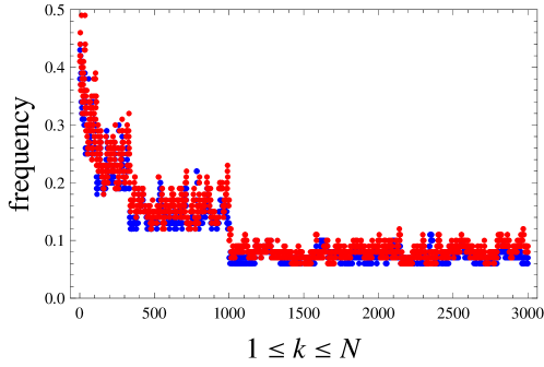
(b) Blue points: frequency in the time-interval $[0,100]$ for the same parameters as in Figs. 2. Red points: the same initial parameters and the same initial activity as for the blue points, but with noise $\eta=0.0001$; cf. Eqs. (6, 7). The blue and red stripes largely overlap, but the red stripe is more narrow, hence the blue points border from below each stripe of red points. There is an approximate correspondence between the noisy and noiseless situations.

Figure 8: (Color Online) Red points (lowest bands for each stripe) are the same as in Fig. 6. Blue points (upper bands for each stripe): the same situation, but with randomly added 1050 links that define 1050 triangles. For each stripe a narrow band of red points borders from below the wider band of blue points. The structure of clusters stays unchanged, but the activity increases after adding triangles.

Figure 9: (Color Online) Frozen random weights. For all figures $q=0.32$, $\kappa=0.101$, $u=1$, $r=0.1$, $K=3$, $N=6\times 10^{3}+1$ (total number of agents). The initial condition was generated with $b=1.8$; see Eq. (16). The random weights were generated with $b^{\prime}=10$; see Eq. (23).
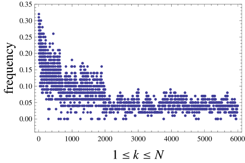
(a) Short-time frequencies: the number of firing for each agent in the time-interval $[800,900]$ divided over the interval length $100$.
(b) Long-time frequencies (in the same situation as (a)): the number of firing for each agent in the time-interval $[900,1300]$ divided over the interval length $400$.

Figure 10: (Color Online) Frozen random weights. For both figures $q=0.29$, $\kappa=0.101$, $u=1$, $r=0.1$, $K=3$, $N=12\times 10^{3}+1$ (total number of agents). The initial condition was generated with $b=1.8$; see Eq. (16). The random weights were generated with $b^{\prime}=10$; see Eq. (23). Frequencies: the number of firing for each agent in the time-interval $[800,1600]$ divided over the interval length $800$.

Figure 11: (Color Online) Annealed random weights. For all figures $u=1$, $\kappa=0.101$, $r=0.1$, $K=3$, $N=6\times 10^{3}+1$ (total number of agents). The initial condition was generated with $b=1.8$; see Eq. (16). The random weights were generated with $b^{\prime}=10$; see Eq. (23).
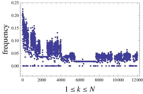
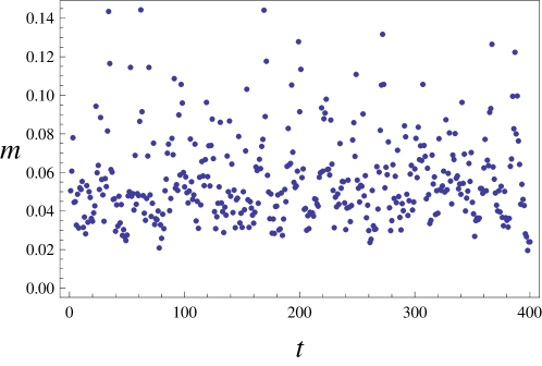
(a) Frequency (long-time) of each agent versus the agent number for $q=0.32$. Frequencies are counted as the number of firing for each agent in the in the time-interval $[400,800]$ divided over the interval length $400$.
(b) The colective activity $m(t)=\frac{1}{N}\sum_{k=1}^{N}m_{i}(t)$ versus discrete time $400+t$ for the same parameters as in (a).

Figure 12: (Color Online) The same parameters as in Figs. 11 and 11.
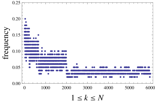
(a) Frequency (short-time) of each agent versus the agent number $q=0.279$. Frequencies are counted as the number of firing for each agent in the in the time-interval $[300,400]$ divided over the interval length $100$.
(b) The colective activity $m(t)=\frac{1}{N}\sum_{k=1}^{N}m_{i}(t)$ versus discrete time $400+t$ for the same parameters as in (a).