11institutetext: Alaa Armiti-Juber/ Christian Rohde
11email: a.armiti/ crohde@mathematik.uni-stuttgart.de
22institutetext: Institute for Applied Analysis and Numerical Simulation, University of Stuttgart, Pfaffenwaldring 57, 70569 Stuttgart, Germany

On Darcy-and Brinkman-Type Models for Two-Phase Flow in Asymptotically Flat Domains

Alaa Armiti-Juber    Christian Rohde
Abstract

We study two-phase flow for Darcy and Brinkman regimes. To reduce the computational complexity for flow in vertical equilibrium various simplified models have been suggested. Examples are dimensional reduction by vertical integration, the multiscale model approach in [Guo et al., 2014] or the asymptotic approach in [Yortsos, 1995]. The latter approach uses a geometrical scaling. We show the efficiency of the approach in asymptotically flat domains for Darcy regimes. Moreover, we prove that it is vastly equivalent to the multiscale model approach.

We apply then asymptotic analysis to the two-phase flow model in Brinkman regimes. The limit model is a single nonlocal evolution law with a pseudo-parabolic extension. Its computational efficiency is demonstrated using numerical examples. Finally, we show that the new limit model exhibits overshoot behaviour as it has been observed for dynamical capillarity laws [Hassanizadeh and Gray, 1993].

Keywords:
Two-phase flow Asymptotically flat domains Vertical equilibrium Model reduction Saturation overshoots in porous media

1 Introduction

In this paper we consider incompressible two-phase flow through a porous medium. If capillary forces are neglected two-phase flow processes are governed by hyperbolic equations for saturation and elliptic Darcy-like laws for the pressure Bear1972 ; Helmig1997 , resulting in a strongly coupled nonlinear system of differential equations. Standard discretization techniques (based on e.g. the implicit pressure and explicit saturation (IMPES) treatment) are computationally quite expensive in spatially three-dimensional settings HuberHelmig1999 . Therefore it is an important issue to perform model reductions if possible, in particular for any kinds of limit regimes.

Here, we focus on porous media in asymptotically flat domains with almost horizontal fluid flow. If the fluids in the domain segregate fast, their pressures can be assumed to be essentially hydrostatic. This assumption is called the vertical equilibrium assumption (the name of this assumption should not be mixed up with the Vertical Equilibrium model presented later). It usually applies to asymptotically flat domains as well as to domains with very high vertical permeability where vertical forces, like gravity, equilibrate very fast.

The vertical equilibrium assumption has been utilized by many researchers to integrate the three-dimensional two-phase flow model over the vertical coordinate and consequently to reduce the computational complexity of the model by dimensional reduction. For example, we refer to Lake1989 in the field of petroleum studies and to Bear1972 ; Helmig1997 in the field of hydrogeology, where the assumption is well-known under the name of Dupuit’s assumption. Recently, this approach has received attention in the field of CO2subscriptCO2\text{CO}_{2}-sequestration in saline aquifers Becker ; Gasda2009 ; Gasda2011 .

Such vertically integrated models have the tendency to overestimate horizontal spreading speeds, mainly in domains where the vertical equilibrium assumption is not fully satisfied court2012 . Examples are heterogeneous porous media with low vertical permeability, media with relatively large thickness and cases when the flowing fluids have a small difference in their densities. Therefore, different approaches that modify the vertical integration approach have been developed. For example, a Multiscale model that relaxes the vertical equilibrium assumption is proposed in Guo2014 . This model consists of a coarse scale vertically integrated equation for the vertically integrated pressure in the horizontal plane and a set of fine scale one-dimensional equations for saturation in the vertical direction. The two equations are coupled via an operator that reconstructs the coarse scale pressure along the vertical coordinate. Another approach for multi-layered flat domains is proposed in Qin2014 . In this approach, the dynamics in each layer is described by a macroscale thickness-integrated mass balance equation coupled by appropriate exchange terms.

In this paper we exploit a model reduction approach of Yortsos Yortsos that relies on asymptotic analysis in terms of the height-length ratio of the domain. The reduced two-phase model is still posed in the fully-dimensional domain but consists of a single nonlocal equation for the saturation alone. We consider this approach for two different two-phase flow scenarios:

  • Asymptotically flat domains with the total velocity satisfying a Darcy-type law.

  • Asymptotically flat domains with the total velocity obeying Brinkman’s equations.

As mentioned above this approach has been explored by Yortsos for a two-phase Darcy-type flow model Yortsos , motivated by the numerical results in Coats1971 ; YokoyamaLake1981 ; ZaptaLake1981 . He called this model the Vertical Equilibrium model. This model has been further investigated to develop selection principles for finding upper bounds on the speed of the mixing zone in the case of miscible displacement MenonOtto2005 ; YortsosSalin2006 . Existence of weak solutions for a regularization of the model in the framework of functions of bounded variations is proved in Armiti-Juber2014 . For miscible displacement in the gap of a planar Hele-Shaw or a long cylindrical capillary, the validity of this model is investigated in Yang1997 . A similar model is developed for layered reservoirs in Zhang2011 ; Zhang2012 . For media with parallel layers of contrasting porosity, absolute permeability and relative permeability, a generalization of the model is proposed in Debbabi2017 .

We first suggest a conservative and stable finite-volume scheme for the nonlocal Vertical Equilibrium model. We show by numerical experiments that the Vertical Equilibrium model is much more accurate than vertically integrated models while still being computationally much more efficient than the full two-phase flow model. In addition to this, we show that the Vertical Equilibrium model and the Multiscale model proposed in Guo2014 coincide in general. This surprising result might lead to further reduction in the computational complexity of the Multiscale model.

In flat domains, we apply asymptotic analysis to the two-phase flow model with the second-order Brinkman’s equations following Yortsos . By doing this, we derive a nonlocal evolution equation for saturation only. It involves additionally a third-order term with mixed –time and spatial– derivatives. We propose a new numerical scheme and show again by numerical examples that this Brinkman Vertical Equilibrium model is in excellent agreement with the full two-phase flow model in flat domains, while being computationally much more efficient.

The Brinkman Vertical Equilibrium model resembles the third-order pseudo-parabolic model proposed in HG1993 and mathematically analyzed in FanPop2010 ; vanDuijn2013 . This model has been derived in a completely other context to model rate-dependent capillarity pressures. In particular, it has been shown (see e.g. vanDuijn2013 ) that it supports the upset of overshooting of invading wetting fronts. We also observe overshooting in the Brinkman Vertical Equilibrium model without introducing additional second gradient forces like in HG1993 .

We conclude the introduction with an overview of the paper’s content: In Section 2 we review the models that describe two-phase flow in asymptotically flat domains. Section 3 provides several comparison examples of the Vertical Equilibrium model with the other models presented in the previous section. In Section 4, we derive the Brinkman Vertical Equilibrium model to describe two-phase flow in flat domains. Section 5 provides a set of numerical tests that show the accuracy and the computational efficiency of the Brinkman Vertical Equilibrium model and its ability to support overshooting fronts.

2 Models for Two-Phase Darcy Flow in Asymptotically Flat Domains

To study fluid flow in porous media on the macroscale physical properties of the phases are averaged over an appropriate control volume, the representative elementary volume Helmig1997 . On this scale, the averaged velocity of the fluids can be described by Darcy’s law.

In this section, we present first the governing equations for a two-phase flow model on the macroscale in a bounded domain Ω3Ωsuperscript3\Omega\subset\mathbb{R}^{3}. Then, we review three different models for asymptotically flat domains: a Vertically Integrated model, the Multiscale model proposed by Guo et al. Guo2014 and the Vertical Equilibrium model proposed by Yortsos Yortsos .

ΩinflowsubscriptΩinflow\partial\Omega_{\text{inflow}}ΩoutflowsubscriptΩoutflow\partial\Omega_{\text{outflow}}ΩimpsubscriptΩimp\partial\Omega_{\text{imp}}ΩimpsubscriptΩimp\partial\Omega_{\text{imp}}LHΩvsubscriptΩ𝑣\Omega_{v}
Figure 1: An illustration of the displacement process in a vertical-cross section ΩvsubscriptΩ𝑣\Omega_{v} of a three-dimensional domain ΩΩ\Omega. For an asymptotically flat domain, the ratio H/L𝐻𝐿H/L tends to zero.

2.1 The Two-Phase Flow Model in the Fully-Dimensional Domain ΩΩ\Omega

In the saturated case, the two-phase flow model (TP-model) is a combination of the continuity equation, Darcy’s law, and the incompressibility relation Helmig1997 , i.e.,

ϕtSα+vα=0,vα=λα(Sα)K(pαραgez),v=0italic-ϕsubscript𝑡subscript𝑆𝛼subscriptv𝛼absent0subscriptv𝛼absentsubscript𝜆𝛼subscript𝑆𝛼Ksubscript𝑝𝛼subscript𝜌𝛼𝑔subscripte𝑧vabsent0\left.\begin{array}[]{rl}\phi\partial_{t}S_{\alpha}+\nabla\cdot\textbf{v}_{\alpha}=&0,\\ \textbf{v}_{\alpha}=&-\lambda_{\alpha}(S_{\alpha})\textbf{K}\left(\nabla p_{\alpha}-\rho_{\alpha}g\textbf{e}_{z}\right),\\ \nabla\cdot\textbf{v}=&0\end{array}\right. (1)

in Ω×(0,T)Ω0𝑇\Omega\times(0,T) for both, the invading α=i𝛼𝑖\alpha=i and the defending α=d𝛼𝑑\alpha=d phase. The unknowns in (1) are the saturation Si=Si(x,y,z,t)[0,1]subscript𝑆𝑖subscript𝑆𝑖𝑥𝑦𝑧𝑡01S_{i}=S_{i}(x,y,z,t)\in[0,1] and the pressure pi=pi(x,y,z,t)subscript𝑝𝑖subscript𝑝𝑖𝑥𝑦𝑧𝑡p_{i}=p_{i}(x,y,z,t)\in\mathbb{R}. Saturation and pressure of the defending phase are then computed using the closure relations Si+Sd=1subscript𝑆𝑖subscript𝑆𝑑1S_{i}+S_{d}=1 and pdpi=pcsubscript𝑝𝑑subscript𝑝𝑖subscript𝑝𝑐p_{d}-p_{i}=p_{c}, respectively, where the capillary pressure pcsubscript𝑝𝑐p_{c} can be assumed to be a given function of saturation of the invading phase Genuchten1980 , pc=pc(Si)subscript𝑝𝑐subscript𝑝𝑐subscript𝑆𝑖p_{c}=p_{c}(S_{i}). The total velocity v=v(x,y,z,t)3vv𝑥𝑦𝑧𝑡superscript3\textbf{v}=\textbf{v}(x,y,z,t)\in\mathbb{R}^{3}, for any (x,y,z,t)Ω×[0,T]𝑥𝑦𝑧𝑡Ω0𝑇(x,y,z,t)\in\Omega\times[0,T], is the sum of the phases’ velocities v=vi+vdvsubscriptv𝑖subscriptv𝑑\textbf{v}=\textbf{v}_{i}+\textbf{v}_{d}. It consists of two horizontal components (u,v)𝑢𝑣(u,v) and one vertical component (w)𝑤(w), i.e., v=(u,v,w)Tvsuperscript𝑢𝑣𝑤𝑇\textbf{v}=(u,v,w)^{T}. The intrinsic permeability tensor

K=K(x,y,z)=(Kx(x,y,z)000Ky(x,y,z)000Kz(x,y,z)),KK𝑥𝑦𝑧subscript𝐾𝑥𝑥𝑦𝑧000subscript𝐾𝑦𝑥𝑦𝑧000subscript𝐾𝑧𝑥𝑦𝑧\displaystyle\textbf{K}=\textbf{K}(x,y,z)=\left(\begin{array}[]{c c c}K_{x}(x,y,z)&0&0\\ 0&K_{y}(x,y,z)&0\\ 0&0&K_{z}(x,y,z)\end{array}\right), (5)

is given with Kx,Kysubscript𝐾𝑥subscript𝐾𝑦K_{x},\,K_{y} and Kzsubscript𝐾𝑧K_{z} being the permeabilities in x𝑥x-, y𝑦y-, and z𝑧z-directions. ϕ=ϕ(x,y,z)[0,1]italic-ϕitalic-ϕ𝑥𝑦𝑧01\phi=\phi(x,y,z)\in[0,1] is the medium’s porosity, ραsubscript𝜌𝛼\rho_{\alpha} is the phase density, g𝑔g is the gravitational acceleration, and ez=(0,0,1)Tsubscripte𝑧superscript001𝑇\textbf{e}_{z}=(0,0,1)^{T}. The phase mobility λα:[0,1][0,):subscript𝜆𝛼010\lambda_{\alpha}:[0,1]\rightarrow[0,\infty) is given by λα(Sα):=krα(Sα)/μαassignsubscript𝜆𝛼subscript𝑆𝛼subscript𝑘𝑟𝛼subscript𝑆𝛼subscript𝜇𝛼\lambda_{\alpha}(S_{\alpha}):=k_{r\alpha}(S_{\alpha})/\mu_{\alpha}, where krαsubscript𝑘𝑟𝛼k_{r\alpha} is the phase relative permeability and the constant μα>0subscript𝜇𝛼0\mu_{\alpha}>0 is the phase viscosity.

For later purpose, we introduce the sum of the phases’ mobilities, called the total mobility λtot=λi+λdsubscript𝜆𝑡𝑜𝑡subscript𝜆𝑖subscript𝜆𝑑\lambda_{tot}=\lambda_{i}+\lambda_{d}. The fractional flow function for the invading phase is defined as f=λiλtot𝑓subscript𝜆𝑖subscript𝜆𝑡𝑜𝑡f=\tfrac{\lambda_{i}}{\lambda_{tot}}. Using quadratic relative permeabilities results in the specific choice

f(Si)=MSi2MSi2+(1Si)2,λtot(Si)=MSi2+(1Si)2.formulae-sequence𝑓subscript𝑆𝑖𝑀superscriptsubscript𝑆𝑖2𝑀superscriptsubscript𝑆𝑖2superscript1subscript𝑆𝑖2subscript𝜆𝑡𝑜𝑡subscript𝑆𝑖𝑀superscriptsubscript𝑆𝑖2superscript1subscript𝑆𝑖2\displaystyle f(S_{i})=\dfrac{MS_{i}^{2}}{MS_{i}^{2}+(1-S_{i})^{2}},\quad\lambda_{tot}(S_{i})=MS_{i}^{2}+(1-S_{i})^{2}. (6)

Here Mμd/μi𝑀subscript𝜇𝑑subscript𝜇𝑖M\coloneqq\mu_{d}/\mu_{i} is the viscosity ratio of the defending phase and the invading phase.

The domain Ω3Ωsuperscript3\Omega\subset\mathbb{R}^{3} is initially saturated with a resident saturation Sdsubscript𝑆𝑑S_{d}. The boundary ΩΩ\partial\Omega, as illustrated in Figure 1, is decomposed into an inflow boundary ΩinflowsubscriptΩinflow\partial\Omega_{\text{inflow}}, an outflow boundary ΩinflowsubscriptΩinflow\partial\Omega_{\text{inflow}} and an impermeable boundary ΩimpsubscriptΩimp\partial\Omega_{\text{imp}}. The initial and boundary conditions are summarized as follows

Si(,,,0)=0, in Ω,Si=Sinflow, on Ωinflow×[0,T],nvα=0, on Ωimp×[0,T],subscript𝑆𝑖0absent0 in Ωsubscript𝑆𝑖absentsubscript𝑆inflow on subscriptΩinflow0𝑇nsubscriptv𝛼absent0 on subscriptΩimp0𝑇\displaystyle\begin{array}[]{rll}S_{i}(\cdot,\cdot,\cdot,0)&=0,&\text{ in }\Omega,\\ S_{i}&=S_{\text{inflow}},&\text{ on }\partial\Omega_{\text{inflow}}\times[0,T],\\ \textbf{n}\cdot\textbf{v}_{\alpha}&=0,&\text{ on }\partial\Omega_{\text{imp}}\times[0,T],\end{array} (10)

where Sinflow[0,1]subscript𝑆inflow01S_{\text{inflow}}\in[0,1] and n denotes the outer normal vector of the boundary ΩimpsubscriptΩimp\partial\Omega_{\text{imp}}. Throughout the paper, the following assumptions are imposed:

Assumption 2.1
  1. 1.

    The permeability components Kx=Ky=Kzsubscript𝐾𝑥subscript𝐾𝑦subscript𝐾𝑧K_{x}=K_{y}=K_{z} in (5) are strictly positive and bounded.

  2. 2.

    There exists a constant c>0𝑐0c>0 s.t. 0Hϕ(,,z)𝑑z>csuperscriptsubscript0𝐻italic-ϕ𝑧differential-d𝑧𝑐\int_{0}^{H}\phi(\cdot,\cdot,z)\,dz>c.

  3. 3.

    For the total mobility λtot=λtot(Si)C2([0,1])subscript𝜆𝑡𝑜𝑡subscript𝜆𝑡𝑜𝑡subscript𝑆𝑖superscript𝐶201\lambda_{tot}=\lambda_{tot}(S_{i})\in C^{2}([0,1]) there is a constant a>0𝑎0a>0 with 0<a<λtot0𝑎subscript𝜆𝑡𝑜𝑡0<a<\lambda_{tot}.

  4. 4.

    The fractional flow f=f(Si)C2([0,1])𝑓𝑓subscript𝑆𝑖superscript𝐶201f=f(S_{i})\in C^{2}([0,1]) is monotone increasing.

2.2 The Vertically Integrated Model

x𝑥x-directionz𝑧z-direction00H𝐻HL𝐿LΩvsubscriptΩ𝑣\Omega_{v}
x𝑥x-directiony𝑦y-directionΩho,inflowsubscriptΩ𝑜inflow\Omega_{ho,\text{inflow}}ΩhosubscriptΩ𝑜\Omega_{ho}Ωho,impsubscriptΩ𝑜imp\partial\Omega_{ho,\text{imp}}Ωho,impsubscriptΩ𝑜imp\partial\Omega_{ho,\text{imp}}
Figure 2: A vertical-cross section of a 3D domain with bottom (0,L)×{0}0𝐿0(0,L)\times\{0\} and top (0,L)×{H}0𝐿𝐻(0,L)\times\{H\} (left). A horizontal-cross section ΩhosubscriptΩ𝑜\Omega_{ho} of a three-dimensional domain ΩΩ\Omega (right).

In the following, we recall the Vertically Integrated model (VI-model) for two-phase flow, see for example Gasda2009 ; Gasda2011 ; Guo2014 . For this, we define the vertically averaged quantities

ϕ^(x,y)=0Hϕ(x,y,z)𝑑z,v^ho,α=0Hvho,α𝑑z,S^α(x,y,t)=1ϕ^0Hϕ(x,y,z)Sα(x,y,z,t)𝑑z,K^(x,y)=0HK(x,y,z)𝑑z,λ^α=K^10HKλα𝑑z.^italic-ϕ𝑥𝑦absentsuperscriptsubscript0𝐻italic-ϕ𝑥𝑦𝑧differential-d𝑧subscript^v𝑜𝛼superscriptsubscript0𝐻subscriptv𝑜𝛼differential-d𝑧subscript^𝑆𝛼𝑥𝑦𝑡absent1^italic-ϕsuperscriptsubscript0𝐻italic-ϕ𝑥𝑦𝑧subscript𝑆𝛼𝑥𝑦𝑧𝑡differential-d𝑧^K𝑥𝑦absentsuperscriptsubscript0𝐻K𝑥𝑦𝑧differential-d𝑧subscript^𝜆𝛼superscript^K1superscriptsubscript0𝐻Ksubscript𝜆𝛼differential-d𝑧\displaystyle\begin{array}[]{rl}\hat{\phi}(x,y)=&\displaystyle{\int_{0}^{H}}\phi(x,y,z)\,dz,\hskip 14.22636pt\hat{\textbf{v}}_{ho,\alpha}=\displaystyle{\int_{0}^{H}}\textbf{v}_{ho,\alpha}\,dz,\vspace{5pt}\\ \hat{S}_{\alpha}(x,y,t)=&\dfrac{1}{\hat{\phi}}\displaystyle{\int_{0}^{H}}\phi(x,y,z)S_{\alpha}(x,y,z,t)\,dz,\vspace{5pt}\\ \widehat{\textbf{K}}(x,y)=&\displaystyle{\int_{0}^{H}}\textbf{K}(x,y,z)\,dz,\hskip 14.22636pt\hat{\lambda}_{\alpha}=\widehat{\textbf{K}}^{-1}\displaystyle{\int_{0}^{H}}\textbf{K}\lambda_{\alpha}\,dz.\end{array} (14)

The vector vho,α=(uα,vα)Tsubscriptv𝑜𝛼superscriptsubscript𝑢𝛼subscript𝑣𝛼𝑇\textbf{v}_{ho,\alpha}=(u_{\alpha},v_{\alpha})^{T} is the velocity vector in the horizontal directions. Assuming that the fluids are in vertical equilibrium means that the phases’ pressures pα,α{i,d}subscript𝑝𝛼𝛼𝑖𝑑p_{\alpha},\,\alpha\in\{i,d\}, are essentially hydrostatic Guo2014 , i.e.

pα(x,y,z,t)=p^α(x,y,t)+ραgz,subscript𝑝𝛼𝑥𝑦𝑧𝑡subscript^𝑝𝛼𝑥𝑦𝑡subscript𝜌𝛼𝑔𝑧\displaystyle p_{\alpha}(x,y,z,t)=\hat{p}_{\alpha}(x,y,t)+\rho_{\alpha}gz, (15)

where p^αsubscript^𝑝𝛼\hat{p}_{\alpha} is the phase reference pressure at the bottom of the medium. Integrating the two-phase flow model (1) along the vertical coordinate from 00 to H𝐻H (Figure 2) and using the vertical equilibrium assumption (15) yields

ϕ^tS^α+hov^ho,α=0,v^ho,α=λ^αK^hop^α,hov^ho=0^italic-ϕsubscript𝑡subscript^𝑆𝛼subscript𝑜subscript^v𝑜𝛼absent0subscript^v𝑜𝛼absentsubscript^𝜆𝛼^Ksubscript𝑜subscript^𝑝𝛼subscript𝑜subscript^v𝑜absent0\displaystyle\begin{array}[]{rl}\hat{\phi}\partial_{t}\hat{S}_{\alpha}+\nabla_{ho}\cdot\hat{\textbf{v}}_{ho,\alpha}&=0,\vspace{5pt}\\ \hat{\textbf{v}}_{ho,\alpha}&=-\hat{\lambda}_{\alpha}\widehat{\textbf{K}}\nabla_{ho}\hat{p}_{\alpha},\vspace{5pt}\\ \nabla_{ho}\cdot\hat{\textbf{v}}_{ho}&=0\end{array} (19)

in Ωho×(0,T)subscriptΩ𝑜0𝑇\Omega_{ho}\times(0,T), where ΩhosubscriptΩ𝑜\Omega_{ho} is a horizontal cross-section of the three-dimensional domain ΩΩ\Omega, see Figure 2, with vertically averaged properties like porosity and permeability. We call this model Vertically Integrated model (VI-model). In this model, v^ho=v^ho,i+v^ho,dsubscript^v𝑜subscript^v𝑜𝑖subscript^v𝑜𝑑\hat{\textbf{v}}_{ho}=\hat{\textbf{v}}_{ho,i}+\hat{\textbf{v}}_{ho,d} is the averaged total velocity and ho=(x,y)Tsubscript𝑜superscriptsubscript𝑥subscript𝑦𝑇\nabla_{ho}=(\partial_{x},\,\partial_{y})^{T} is the gradient operator in the horizontal x𝑥x- and y𝑦y-directions. The VI-model has two unknowns: the averaged saturation S^i=S^i(x,y,t)[0,1]subscript^𝑆𝑖subscript^𝑆𝑖𝑥𝑦𝑡01\hat{S}_{i}=\hat{S}_{i}(x,y,t)\in[0,1] and the averaged pressure p^i=p^i(x,y,t)subscript^𝑝𝑖subscript^𝑝𝑖𝑥𝑦𝑡\hat{p}_{i}=\hat{p}_{i}(x,y,t)\in\mathbb{R}. Saturation and pressure of the defending phase can be again computed using the closure relations S^i+S^d=1subscript^𝑆𝑖subscript^𝑆𝑑1\hat{S}_{i}+\hat{S}_{d}=1 and p^dp^i=pc^subscript^𝑝𝑑subscript^𝑝𝑖^subscript𝑝𝑐\hat{p}_{d}-\hat{p}_{i}=\widehat{p_{c}}, where pc^=pc(S^i)^subscript𝑝𝑐subscript𝑝𝑐subscript^𝑆𝑖\widehat{p_{c}}=p_{c}(\hat{S}_{i}), respectively.

The initial and boundary conditions in (10) are also vertically averaged for the VI-model and are given as

S^i(,,0)=0, in Ωho,S^i=S^inflow, in Ωho,inflow×[0,T],nv^ho,α=0, on Ωho,imp×[0,T].subscript^𝑆𝑖0absent0 in subscriptΩ𝑜subscript^𝑆𝑖absentsubscript^𝑆inflow in subscriptΩ𝑜inflow0𝑇nsubscript^v𝑜𝛼absent0 on subscriptΩ𝑜imp0𝑇\displaystyle\begin{array}[]{rll}\hat{S}_{i}(\cdot,\cdot,0)&=0,&\text{ in }\Omega_{ho},\\ \hat{S}_{i}&=\hat{S}_{\text{inflow}},&\text{ in }\partial\Omega_{ho,\text{inflow}}\times[0,T],\\ \textbf{n}\cdot\hat{\textbf{v}}_{ho,\alpha}&=0,&\text{ on }\partial\Omega_{ho,\text{imp}}\times[0,T].\end{array} (23)

In (23), we have S^inflow[0,1]subscript^𝑆inflow01\hat{S}_{\text{inflow}}\in[0,1], and Ωho,inflowsubscriptΩ𝑜inflow\partial\Omega_{ho,\text{inflow}} is the inflow boundary of the horizontal cross-section ΩhosubscriptΩ𝑜\Omega_{ho} (Figure 2).

2.3 The Multiscale Model

Guo et al. Guo2014 proposed a reduced model for asymptotically flat domains which they call the Multiscale model. It is used to describe CO2subscriptCO2\text{CO}_{2} storage whenever the vertical equilibrium assumption (15) is not fully applicable. It comprises two scales: a coarse scale which is a horizontal cross-section ΩhosubscriptΩ𝑜\Omega_{ho} of the three-dimensional domain ΩΩ\Omega, with vertically averaged properties, and a fine scale which is a series of one-dimensional vertical columns across the formation (Figure 3). The governing equations for this model are of two types: a two-dimensional equation for the vertically averaged pressure p^isubscript^𝑝𝑖\hat{p}_{i} (coarse-scale pressure Guo2014 ), as in the VI-model (19), and the two-phase flow model (1) for the saturation (fine-scale saturation Guo2014 ), rearranged to focus on the vertical dynamics. These two type of equations are connected using an operator that reconstructs the coarse-scale pressure along the vertical direction.

x𝑥x-directiony𝑦y-directionΩho,inflowsubscriptΩ𝑜inflow\Omega_{ho,\text{inflow}}ΩhosubscriptΩ𝑜\Omega_{ho}coarse scalez𝑧z-directionfine scale
Figure 3: An illustration of the two scales in the Multiscale model: the coarse-scale is the horizontal xy𝑥𝑦xy-plane while the fine-scale is a series of one-dimensional vertical domains. The arrows refer to the flow direction in the corresponding domains.

The Multiscale model is summarized for the invading phase α=i𝛼𝑖\alpha=i as follows:

hoK^(λtot(S^i)hop^i)subscript𝑜^Ksubscript𝜆𝑡𝑜𝑡subscript^𝑆𝑖subscript𝑜subscript^𝑝𝑖\displaystyle-\nabla_{ho}\cdot\widehat{\textbf{K}}\bigl{(}\lambda_{tot}(\hat{S}_{i})\nabla_{ho}\hat{p}_{i}\bigr{)} =hoK^(λ^d(S^i)hop^c(S^i))absentsubscript𝑜^Ksubscript^𝜆𝑑subscript^𝑆𝑖subscript𝑜subscript^𝑝𝑐subscript^𝑆𝑖\displaystyle=\nabla_{ho}\cdot\widehat{\textbf{K}}\bigl{(}\hat{\lambda}_{d}(\hat{S}_{i})\nabla_{ho}\widehat{p}_{c}(\hat{S}_{i})\bigr{)} (24)

in Ωho×(0,T)subscriptΩ𝑜0𝑇\Omega_{ho}\times(0,T), and

pi=p^i+πi,vho,i=λi(Si)Khopi,zw=hovho,wi=f(Si)w+f(Si)λd(Si)Kz(zpc(Si)+(ρiρd)g),ϕtSi+vi=0\displaystyle\begin{array}[]{rl}p_{i}=&\hat{p}_{i}+\pi_{i},\\ \textbf{v}_{ho,i}=&-\lambda_{i}(S_{i})\textbf{K}_{ho}\nabla p_{i},\\ \partial_{z}w=&-\nabla_{ho}\cdot\textbf{v}_{ho},\\ w_{i}=&f(S_{i})w+f(S_{i})\lambda_{d}(S_{i})K_{z}\big{(}\partial_{z}p_{c}(S_{i})\\ &+(\rho_{i}-\rho_{d})g\big{)},\\ \phi\partial_{t}S_{i}+\nabla\cdot\textbf{v}_{i}=&0\end{array} (31)

in Ω×(0,T)Ω0𝑇\Omega\times(0,T). Referencing to Guo2014 , a preferred choice of the reconstruction operator πisubscript𝜋𝑖\pi_{i}, that is simple to compute and represents the natural forces in the medium, is given by

πi(x,y,z,t)=subscript𝜋𝑖𝑥𝑦𝑧𝑡\displaystyle\pi_{i}(x,y,z,t)=- 0z((Si(x,y,r,t)ρi+(1Si(x,y,r,t))ρd)g\displaystyle\displaystyle{\int_{0}^{z}}\Big{(}\big{(}S_{i}(x,y,r,t)\rho_{i}+(1-S_{i}(x,y,r,t))\rho_{d}\big{)}g
+\displaystyle+ Si(x,y,r,t)pc(1Si(x,y,r,t))z)dr,\displaystyle S_{i}(x,y,r,t)\frac{\partial p_{c}\big{(}1-S_{i}(x,y,r,t)\big{)}}{\partial_{z}}\Big{)}dr, (32)

for any (x,y,z)Ω𝑥𝑦𝑧Ω(x,y,z)\in\Omega and t(0,T)𝑡0𝑇t\in(0,T). The unknowns in this model are the vertically averaged pressure p^i=p^i(x,y,t)subscript^𝑝𝑖subscript^𝑝𝑖𝑥𝑦𝑡\hat{p}_{i}=\hat{p}_{i}(x,y,t)\in\mathbb{R} and the saturation Si=Si(x,y,z,t)[0,1]subscript𝑆𝑖subscript𝑆𝑖𝑥𝑦𝑧𝑡01S_{i}=S_{i}(x,y,z,t)\in[0,1].

Note that the first equation in (31) with the choice of πisubscript𝜋𝑖\pi_{i} in (32) substitutes the vertical equilibrium assumption (15) in the VI-model. The Multiscale model (24), (31) is closed with the initial and boundary conditions

S^i(,,0)=0, in Ωho,S^i=S^inflow, in Ωho,inflow×[0,T],Si(,,,0)=0, in Ω,Si=Sinflow, in Ωinflow×[0,T],nvi=0, in Ωimp×[0,T].subscript^𝑆𝑖0absent0 in subscriptΩ𝑜subscript^𝑆𝑖absentsubscript^𝑆inflow in subscriptΩ𝑜inflow0𝑇subscript𝑆𝑖0absent0 in Ωsubscript𝑆𝑖absentsubscript𝑆inflow in subscriptΩinflow0𝑇nsubscriptv𝑖absent0 in subscriptΩimp0𝑇\displaystyle\begin{array}[]{rll}\hat{S}_{i}(\cdot,\cdot,0)&=0,&\text{ in }\Omega_{ho},\\ \hat{S}_{i}&=\hat{S}_{\text{inflow}},&\text{ in }\partial\Omega_{ho,\text{inflow}}\times[0,T],\\ S_{i}(\cdot,\cdot,\cdot,0)&=0,&\text{ in }\Omega,\\ S_{i}&=S_{\text{inflow}},&\text{ in }\partial\Omega_{\text{inflow}}\times[0,T],\\ \textbf{n}\cdot\textbf{v}_{i}&=0,&\text{ in }\partial\Omega_{\text{imp}}\times[0,T].\end{array} (38)

2.4 The Vertical Equilibrium Model

Yortsos Yortsos proposed the Vertical Equilibrium model (VE-model) to describe displacement processes in a vertical cross-section Ωv=(0,L)×(0,H)subscriptΩ𝑣0𝐿0𝐻\Omega_{v}=(0,L)\times(0,H) of an asymptotically flat domain Ω3Ωsuperscript3\Omega\subset\mathbb{R}^{3} such that the horizontal coordinate is parallel to the injection direction (Figure 1).

We consider the model under the assumption of negligible gravity and capillary forces. First, we set γH/L𝛾𝐻𝐿\gamma\coloneqq H/L and rescale the variables x,y,t,Kx,Kz,pα𝑥𝑦𝑡subscript𝐾𝑥subscript𝐾𝑧subscript𝑝𝛼x,y,t,K_{x},K_{z},p_{\alpha} in (1) into the dimensionless ones

x¯=xL,z¯=zH,t¯=tL/q,κj=Kjkju¯α=uαq,w¯α=wαq,p¯α=pαLqμd/k1,¯𝑥absent𝑥𝐿¯𝑧absent𝑧𝐻¯𝑡absent𝑡𝐿𝑞subscript𝜅𝑗absentsubscript𝐾𝑗subscript𝑘𝑗subscript¯𝑢𝛼absentsubscript𝑢𝛼𝑞subscript¯𝑤𝛼absentsubscript𝑤𝛼𝑞subscript¯𝑝𝛼absentsubscript𝑝𝛼𝐿𝑞subscript𝜇𝑑subscript𝑘1missing-subexpressionmissing-subexpression\begin{array}[]{rlrlrlrl}\overline{x}=&\dfrac{x}{L},&\overline{z}=&\dfrac{z}{H},&\overline{t}=&\dfrac{t}{L/q},&\kappa_{j}=&\dfrac{K_{j}}{k_{j}}\\ \overline{u}_{\alpha}=&\dfrac{u_{\alpha}}{q},&\overline{w}_{\alpha}=&\dfrac{w_{\alpha}}{q},&\overline{p}_{\alpha}=&\dfrac{p_{\alpha}}{Lq\mu_{d}/k_{1}},\end{array} (39)

for j{x,z}𝑗𝑥𝑧j\in\{x,z\} and α{i,d}𝛼𝑖𝑑\alpha\in\{i,d\}. Here, q>0𝑞0q>0 is the inflow speed at the inflow boundary ΩinflowsubscriptΩinflow\partial\Omega_{\text{inflow}} and kjsubscript𝑘𝑗k_{j} is the mean value of the corresponding permeability function Kjsubscript𝐾𝑗K_{j}. Then, after omitting the bar-signs, the TP-model (1) transforms into

ϕtSα+xuα+1γzwα=0,xu+1γzw=0,uα=λα(Sα)κxpα,γwα=λα(Sα)κzpαitalic-ϕsubscript𝑡subscript𝑆𝛼subscript𝑥subscript𝑢𝛼1𝛾subscript𝑧subscript𝑤𝛼absent0subscript𝑥𝑢1𝛾subscript𝑧𝑤absent0subscript𝑢𝛼absentsubscript𝜆𝛼subscript𝑆𝛼𝜅subscript𝑥subscript𝑝𝛼𝛾subscript𝑤𝛼absentsubscript𝜆𝛼subscript𝑆𝛼𝜅subscript𝑧subscript𝑝𝛼\displaystyle\left.\begin{array}[]{rl}\phi\partial_{t}S_{\alpha}+\partial_{x}u_{\alpha}+\dfrac{1}{\gamma}\partial_{z}w_{\alpha}&=0,\\ \partial_{x}u+\dfrac{1}{\gamma}\partial_{z}w&=0,\\ u_{\alpha}&=-\lambda_{\alpha}(S_{\alpha})\,\kappa\,\partial_{x}p_{\alpha},\\ \gamma w_{\alpha}&=-\lambda_{\alpha}(S_{\alpha})\,\kappa\,\partial_{z}p_{\alpha}\end{array}\right. (44)

in D×(0,T)𝐷0𝑇D\times(0,T), where D(0,1)×(0,1)𝐷0101D\coloneqq(0,1)\times(0,1) is the dimensionless spatial domain and κκx=κz𝜅subscript𝜅𝑥subscript𝜅𝑧\kappa\coloneqq\kappa_{x}=\kappa_{z}, by Assumption 2.1(1). Neglecting the capillary pressure implies pi=pd=:pp_{i}=p_{d}=:p and one can show that the phases’ velocities satisfy

uα=f(Sα)u,wα=f(Sα)w.formulae-sequencesubscript𝑢𝛼𝑓subscript𝑆𝛼𝑢subscript𝑤𝛼𝑓subscript𝑆𝛼𝑤\displaystyle u_{\alpha}=f(S_{\alpha})u,\quad\quad w_{\alpha}=f(S_{\alpha})w.

Then, the dimensionless TP-model (44) is reformulated in the fractional flow formulation with the unknown variables Sαγ,uγ,wγsubscriptsuperscript𝑆𝛾𝛼superscript𝑢𝛾superscript𝑤𝛾S^{\gamma}_{\alpha},\,u^{\gamma},\,w^{\gamma} and pγsuperscript𝑝𝛾p^{\gamma} for some γ>0𝛾0\gamma>0,

ϕtSαγ+x(uγf(Sαγ))+1γz(wγf(Sαγ))=0,x(uγ)+1γz(wγ)=0,uγ=λtot(Sαγ)κxpγ,γwγ=λtot(Sαγ)κzpγitalic-ϕsubscript𝑡subscriptsuperscript𝑆𝛾𝛼subscript𝑥superscript𝑢𝛾𝑓subscriptsuperscript𝑆𝛾𝛼1𝛾subscript𝑧superscript𝑤𝛾𝑓subscriptsuperscript𝑆𝛾𝛼absent0subscript𝑥superscript𝑢𝛾1𝛾subscript𝑧superscript𝑤𝛾absent0superscript𝑢𝛾absentsubscript𝜆𝑡𝑜𝑡subscriptsuperscript𝑆𝛾𝛼𝜅subscript𝑥superscript𝑝𝛾𝛾superscript𝑤𝛾absentsubscript𝜆𝑡𝑜𝑡subscriptsuperscript𝑆𝛾𝛼𝜅subscript𝑧superscript𝑝𝛾\displaystyle\left.\begin{array}[]{rl}\phi\partial_{t}S^{\gamma}_{\alpha}+\partial_{x}(u^{\gamma}f(S^{\gamma}_{\alpha}))+\dfrac{1}{\gamma}\partial_{z}(w^{\gamma}f(S^{\gamma}_{\alpha}))&=0,\\ \partial_{x}(u^{\gamma})+\dfrac{1}{\gamma}\partial_{z}(w^{\gamma})&=0,\\ u^{\gamma}&=-\lambda_{tot}(S^{\gamma}_{\alpha})\kappa\partial_{x}p^{\gamma},\\ \gamma w^{\gamma}&=-\lambda_{tot}(S^{\gamma}_{\alpha})\kappa\partial_{z}p^{\gamma}\end{array}\right. (49)

in D×(0,T)𝐷0𝑇D\times(0,T). Here, uγsuperscript𝑢𝛾u^{\gamma} and wγsuperscript𝑤𝛾w^{\gamma} are the velocity components in the horizontal- and vertical-directions. The unknowns in this model are pressure pγsuperscript𝑝𝛾p^{\gamma} and saturation Sαγsubscriptsuperscript𝑆𝛾𝛼S^{\gamma}_{\alpha} for one of the phases. Yortsos applied formal asymptotic analysis for γ0𝛾0\gamma\rightarrow 0 and eliminated the pressure pγsuperscript𝑝𝛾p^{\gamma} from the velocity (uγ,wγ)superscript𝑢𝛾superscript𝑤𝛾(u^{\gamma},w^{\gamma}) as clarified below.

We assume that for each γ>0𝛾0\gamma>0 there exists a solution (Sγ,pγ,uγ,wγ)superscript𝑆𝛾superscript𝑝𝛾superscript𝑢𝛾superscript𝑤𝛾(S^{\gamma},p^{\gamma},u^{\gamma},w^{\gamma}) of (49), with the asymptotic expansions

Zγ=Z0+γZ1+𝒪(γ2),for Zγ{Sαγ,pγ,uγ},wγ=γw1+𝒪(γ2).superscript𝑍𝛾subscript𝑍0𝛾subscript𝑍1𝒪superscript𝛾2for superscript𝑍𝛾subscriptsuperscript𝑆𝛾𝛼superscript𝑝𝛾superscript𝑢𝛾superscript𝑤𝛾𝛾subscript𝑤1𝒪superscript𝛾2missing-subexpression\displaystyle\begin{array}[]{ll}Z^{\gamma}=Z_{0}+\gamma Z_{1}+\mathcal{O}(\gamma^{2}),&\text{for }Z^{\gamma}\in\{S^{\gamma}_{\alpha},\,p^{\gamma},\,u^{\gamma}\},\vspace{3pt}\\ w^{\gamma}=\gamma w_{1}+\mathcal{O}(\gamma^{2}).\end{array} (52)

Note that the second equation in (52) corresponds to the additional assumption, that the vertical velocity wγsuperscript𝑤𝛾w^{\gamma} is small. Using Assumptions 2.1(3) and 2.1(4), we have

λtot(Sαγ)=λtot(Sα,0)+λtot(Sα,0)(γSα,1)+𝒪(γ2),f(Sαγ)=f(Sα,0)+f(Sα,0)(γSα,1)+𝒪(γ2).subscript𝜆𝑡𝑜𝑡subscriptsuperscript𝑆𝛾𝛼absentsubscript𝜆𝑡𝑜𝑡subscript𝑆𝛼0superscriptsubscript𝜆𝑡𝑜𝑡subscript𝑆𝛼0𝛾subscript𝑆𝛼1𝒪superscript𝛾2𝑓subscriptsuperscript𝑆𝛾𝛼absent𝑓subscript𝑆𝛼0superscript𝑓subscript𝑆𝛼0𝛾subscript𝑆𝛼1𝒪superscript𝛾2\displaystyle\begin{array}[]{rl}\lambda_{tot}(S^{\gamma}_{\alpha})=&\lambda_{tot}(S_{\alpha,0})+\lambda_{tot}^{\prime}(S_{\alpha,0})(\gamma S_{\alpha,1})+\mathcal{O}(\gamma^{2}),\vspace{3pt}\\ f(S^{\gamma}_{\alpha})=&f(S_{\alpha,0})+f^{\prime}(S_{\alpha,0})(\gamma S_{\alpha,1})+\mathcal{O}(\gamma^{2}).\end{array} (55)

The second equation in (49) allows rewriting the first equation in (49) in a nonconservative form. Substituting the expansions (52) and (55) into (49), then considering terms of order 𝒪(1)𝒪1\mathcal{O}(1) in each equation leads to

ϕtSα,0+u0xf(Sα,0)+w1zf(Sα,0)=𝒪(γ),xu0+zw1=𝒪(γ),λtot(Sα,0)κxp0=u0,λtot(Sα,0)κzp0=𝒪(γ).italic-ϕsubscript𝑡subscript𝑆𝛼0subscript𝑢0subscript𝑥𝑓subscript𝑆𝛼0subscript𝑤1subscript𝑧𝑓subscript𝑆𝛼0absent𝒪𝛾subscript𝑥subscript𝑢0subscript𝑧subscript𝑤1absent𝒪𝛾subscript𝜆𝑡𝑜𝑡subscript𝑆𝛼0𝜅subscript𝑥subscript𝑝0absentsubscript𝑢0subscript𝜆𝑡𝑜𝑡subscript𝑆𝛼0𝜅subscript𝑧subscript𝑝0absent𝒪𝛾\displaystyle\begin{array}[]{rl}\phi\partial_{t}S_{\alpha,0}+u_{0}\partial_{x}f(S_{\alpha,0})+w_{1}\partial_{z}f(S_{\alpha,0})=&\mathcal{O}(\gamma),\vspace{3pt}\\ \partial_{x}u_{0}+\partial_{z}w_{1}=&\mathcal{O}(\gamma),\vspace{3pt}\\ -\lambda_{tot}(S_{\alpha,0})\kappa\partial_{x}p_{0}=&u_{0},\vspace{3pt}\\ -\lambda_{tot}(S_{\alpha,0})\kappa\partial_{z}p_{0}=&\mathcal{O}(\gamma).\end{array} (60)

Due to the positivity of λtotsubscript𝜆𝑡𝑜𝑡\lambda_{tot} and κ𝜅\kappa by Assumption 2.1(1) and 2.1(3), the last equation in (60) simplifies to

zp0=𝒪(γ).subscript𝑧subscript𝑝0𝒪𝛾\displaystyle\partial_{z}p_{0}=\mathcal{O}(\gamma). (61)

Thus, as γ0𝛾0\gamma\rightarrow 0, the global pressure p0subscript𝑝0p_{0} is independent of the z𝑧z-coordinate

p0=p0(x,t).subscript𝑝0subscript𝑝0𝑥𝑡\displaystyle p_{0}=p_{0}(x,t). (62)

The result in (62) is a consequence of the asymptotic analysis and substitutes the vertical equilibrium assumption (15) in the VI-model.

In the following, the result (62) is used to reformulate the velocity v=(u,w)Tvsuperscript𝑢𝑤𝑇\textbf{v}=(u,w)^{T} in terms of saturation only. Integrating the second equation in (60) along the vertical direction from 00 to 111, then using impermeability of the top and the bottom parts Dimpsubscript𝐷imp\partial D_{\text{imp}} of the domain ΩΩ\Omega yields

x01u0(x,z,t)𝑑z=01zw1(x,z,t)dz=0,subscript𝑥superscriptsubscript01subscript𝑢0𝑥𝑧𝑡differential-d𝑧superscriptsubscript01subscript𝑧subscript𝑤1𝑥𝑧𝑡𝑑𝑧0\displaystyle\partial_{x}\int_{0}^{1}u_{0}(x,z,t)\,dz=-\int_{0}^{1}\partial_{z}w_{1}(x,z,t)\,dz=0, (63)

as γ0𝛾0\gamma\rightarrow 0. Thus, we have

01u0𝑑z=h,superscriptsubscript01subscript𝑢0differential-d𝑧\displaystyle\int_{0}^{1}u_{0}dz=h, (64)

for some function h=h(t)𝑡h=h(t) with h(t)>0𝑡0h(t)>0 for all t[0,T]𝑡0𝑇t\in[0,T]. Integrating the third equation in (60) along the vertical direction from 00 to 111, then using equation (64) gives

01λtot(Sα,0(x,z,t))κ(x,z)xp0(x,t)dz=h(t).superscriptsubscript01subscript𝜆𝑡𝑜𝑡subscript𝑆𝛼0𝑥𝑧𝑡𝜅𝑥𝑧subscript𝑥subscript𝑝0𝑥𝑡𝑑𝑧𝑡-\int_{0}^{1}\lambda_{tot}(S_{\alpha,0}(x,z,t))\kappa(x,z)\partial_{x}p_{0}(x,t)\,dz=h(t).

Since p0subscript𝑝0p_{0} is independent of the vertical coordinate z𝑧z we obtain that

xp0(x,t)=h(t)01λtot(Sα,0(x,z,t))κ(x,z)𝑑z.subscript𝑥subscript𝑝0𝑥𝑡𝑡superscriptsubscript01subscript𝜆𝑡𝑜𝑡subscript𝑆𝛼0𝑥𝑧𝑡𝜅𝑥𝑧differential-d𝑧\partial_{x}p_{0}(x,t)=-\dfrac{h(t)}{\int_{0}^{1}\lambda_{tot}(S_{\alpha,0}(x,z,t))\kappa(x,z)\,dz}. (65)

Substituting (65) into the third equation in (60) gives a pressure independent formula for the horizontal velocity component u0subscript𝑢0u_{0},

u0[x,z,t;Sα,0(x,z,t)]=h(t)λtot(Sα,0(x,z,t))κ(x,z)01λtot(Sα,0(x,r,t))κ(x,r)𝑑r,subscript𝑢0𝑥𝑧𝑡subscript𝑆𝛼0𝑥𝑧𝑡𝑡subscript𝜆𝑡𝑜𝑡subscript𝑆𝛼0𝑥𝑧𝑡𝜅𝑥𝑧superscriptsubscript01subscript𝜆𝑡𝑜𝑡subscript𝑆𝛼0𝑥𝑟𝑡𝜅𝑥𝑟differential-d𝑟u_{0}[x,z,t;S_{\alpha,0}(x,z,t)]=\dfrac{h(t)\lambda_{tot}\bigl{(}S_{\alpha,0}(x,z,t)\bigr{)}\kappa(x,z)}{\int_{0}^{1}\lambda_{tot}\bigl{(}S_{\alpha,0}(x,r,t)\bigr{)}\kappa(x,r)\,dr},

for all (x,z)D𝑥𝑧𝐷(x,z)\in D and t(0,T)𝑡0𝑇t\in(0,T). This formula is substituted in the second equation in (60) to produce a pressure independent formula for the vertical velocity component w1subscript𝑤1w_{1},

w1[x,z,t;Sα,0(x,z,t)]=h(t)x0zλtot(Sα,0(x,r,t))κ(x,r)𝑑r01λtot(Sα,0(x,r,t))κ(x,r)𝑑r,subscript𝑤1𝑥𝑧𝑡subscript𝑆𝛼0𝑥𝑧𝑡𝑡subscript𝑥superscriptsubscript0𝑧subscript𝜆𝑡𝑜𝑡subscript𝑆𝛼0𝑥𝑟𝑡𝜅𝑥𝑟differential-d𝑟superscriptsubscript01subscript𝜆𝑡𝑜𝑡subscript𝑆𝛼0𝑥𝑟𝑡𝜅𝑥𝑟differential-d𝑟w_{1}[x,z,t;S_{\alpha,0}(x,z,t)]=-h(t)\partial_{x}\dfrac{\int_{0}^{z}\lambda_{tot}\bigl{(}S_{\alpha,0}(x,r,t)\bigr{)}\kappa(x,r)\,dr}{\int_{0}^{1}\lambda_{tot}\bigl{(}S_{\alpha,0}(x,r,t)\bigr{)}\kappa(x,r)\,dr},

for all (x,z)D𝑥𝑧𝐷(x,z)\in D and t(0,T)𝑡0𝑇t\in(0,T). Rescaling the time using tt¯=0th(r)𝑑r+h(0)tmaps-to𝑡¯𝑡superscriptsubscript0𝑡𝑟differential-d𝑟0𝑡t\mapsto\bar{t}=\int_{0}^{t}h(r)dr+h(0)t, then omitting the subscripts {0,1}01\{0,1\} and the bar-signs yields the VE-model

ϕtSα+x(u[,;Sα]\displaystyle\phi\partial_{t}S_{\alpha}+\partial_{x}\big{(}u[\cdot,\cdot;S_{\alpha}] f(Sα))+z(w[,;Sα]f(Sα))=0,\displaystyle f(S_{\alpha})\big{)}+\partial_{z}\big{(}w[\cdot,\cdot;S_{\alpha}]~{}f(S_{\alpha})\big{)}=0,
u[,;Sα]=𝑢subscript𝑆𝛼absent\displaystyle u[\cdot,\cdot;S_{\alpha}]= λtot(Sα)κ01λtot(Sα(,r,))κ(,r)𝑑r,subscript𝜆𝑡𝑜𝑡subscript𝑆𝛼𝜅superscriptsubscript01subscript𝜆𝑡𝑜𝑡subscript𝑆𝛼𝑟𝜅𝑟differential-d𝑟\displaystyle\dfrac{\lambda_{tot}\bigl{(}S_{\alpha}\bigr{)}\kappa}{\int_{0}^{1}\lambda_{tot}\bigl{(}S_{\alpha}(\cdot,r,\cdot)\bigr{)}\kappa(\cdot,r)\,dr},
w[,z;Sα(,z,)]=𝑤𝑧subscript𝑆𝛼𝑧absent\displaystyle w[\cdot,z;S_{\alpha}(\cdot,z,\cdot)]= x0zλtot(Sα(,r,))κ(,r)𝑑r01λtot(Sα(,r,))κ(,r)𝑑rsubscript𝑥superscriptsubscript0𝑧subscript𝜆𝑡𝑜𝑡subscript𝑆𝛼𝑟𝜅𝑟differential-d𝑟superscriptsubscript01subscript𝜆𝑡𝑜𝑡subscript𝑆𝛼𝑟𝜅𝑟differential-d𝑟\displaystyle-\partial_{x}\dfrac{\int_{0}^{z}\lambda_{tot}\bigl{(}S_{\alpha}(\cdot,r,\cdot)\bigr{)}\kappa(\cdot,r)\,dr}{\int_{0}^{1}\lambda_{tot}\bigl{(}S_{\alpha}(\cdot,r,\cdot)\bigr{)}\kappa(\cdot,r)\,dr} (66)

in D×(0,T)𝐷0𝑇D\times(0,T) for all z(0,1)𝑧01z\in(0,1). It is easy to check that the velocity vector (u,w)Tsuperscript𝑢𝑤𝑇(u,w)^{T} in (66) is divergence free.

The velocity components in (66) depend nonlocally on saturation. Hence, for the numerical comparisons in the next section, we suggest a finite-volume scheme with a non standard numerical flux that accounts for the nonlocality, and preserves the incompressibility property of the velocity.

3 Comparison of the Darcy Models in Asymptotically Flat Domains

In this section, we compare the VE-model (66) with the other models from Section 2. For this, we suggest a stable finite-volume scheme for the nonlocal VE-model. The comparisons show: firstly, the VE-model (66) is more accurate than the VI-model, while being computationally more efficient than the full two-phase flow model. Secondly, the Multiscale model is equivalent to the VE-model in general.

3.1 Finite-Volume Scheme for the VE-Model

We consider a Cartesian grid for the dimensionless domain D=(0,1)2𝐷superscript012D=(0,1)^{2},

𝒯={Ti,j=\displaystyle\mathcal{T}=\big{\{}T_{i,j}= [xi12,xi+12)×[zj12,zj+12)(i,j)x×zconditionalsubscript𝑥𝑖12subscript𝑥𝑖12subscript𝑧𝑗12subscript𝑧𝑗12𝑖𝑗subscript𝑥subscript𝑧absent\displaystyle[x_{i-\frac{1}{2}},x_{i+\frac{1}{2}})\times[z_{j-\frac{1}{2}},z_{j+\frac{1}{2}})\mid(i,j)\in\mathcal{I}_{x}\times\mathcal{I}_{z}\subset
×},\displaystyle\mathbb{N}\times\mathbb{N}\big{\}},

with the set of midpoints {(xi,zj)(i,j)x×z}conditional-setsubscript𝑥𝑖subscript𝑧𝑗𝑖𝑗subscript𝑥subscript𝑧\{(x_{i},z_{j})\mid(i,j)\in\mathcal{I}_{x}\times\mathcal{I}_{z}\}. The set of edges of the cell Ti,jsubscript𝑇𝑖𝑗T_{i,j} is denoted by {El|lθi,j}conditional-setsubscript𝐸𝑙𝑙subscript𝜃𝑖𝑗\{E_{l}~{}|l\in\theta_{i,j}\} where

θi,j:={(i12,j),(i+12,j),(i,j12),(i,j+12)}.assignsubscript𝜃𝑖𝑗𝑖12𝑗𝑖12𝑗𝑖𝑗12𝑖𝑗12\displaystyle\theta_{i,j}:=\left\{\left(i-\frac{1}{2},j\right),\left(i+\frac{1}{2},j\right),\left(i,j-\frac{1}{2}\right),\left(i,j+\frac{1}{2}\right)\right\}.

The set of neighbor cells of Ti,jsubscript𝑇𝑖𝑗T_{i,j} is defined as {T(i,j)llθi,j}conditional-setsubscript𝑇subscript𝑖𝑗𝑙𝑙subscript𝜃𝑖𝑗\{T_{(i,j)_{l}}\mid l\in\theta_{i,j}\}, where T(i,j)lsubscript𝑇subscript𝑖𝑗𝑙T_{(i,j)_{l}} is the neighbor cell to Ti,jsubscript𝑇𝑖𝑗T_{i,j} with the common edge Elsubscript𝐸𝑙E_{l}. Let Nxsubscript𝑁𝑥N_{x} and Nzsubscript𝑁𝑧N_{z} be the number of cells in the horizontal and vertical directions, respectively. Then, the size of a cell is |Ti,j|=ΔxΔzsubscript𝑇𝑖𝑗Δ𝑥Δ𝑧|T_{i,j}|=\Delta x\Delta z, where Δx1NxΔ𝑥1subscript𝑁𝑥\Delta x\coloneqq\tfrac{1}{N_{x}} and Δz1NzΔ𝑧1subscript𝑁𝑧\Delta z\coloneqq\tfrac{1}{N_{z}}. For the initial condition S0[0,1]subscript𝑆001S_{0}\in[0,1], we define the cell-averaged values

Si,j0=1|Ti,j|Ti,jS0(x,z)𝑑x𝑑z,(i,j)x×z.formulae-sequencesuperscriptsubscript𝑆𝑖𝑗01subscript𝑇𝑖𝑗subscriptsubscript𝑇𝑖𝑗subscript𝑆0𝑥𝑧differential-d𝑥differential-d𝑧𝑖𝑗subscript𝑥subscript𝑧\displaystyle S_{i,j}^{0}=\frac{1}{|T_{i,j}|}\int_{T_{i,j}}S_{0}(x,z)\,dx\,dz,\quad\quad(i,j)\in\mathcal{I}_{x}\times\mathcal{I}_{z}. (67)

Given a positive integer N𝑁N, the time interval [0,T]0𝑇[0,T] is discretized into a set of disjoint subintervals [tn,tn+1)superscript𝑡𝑛superscript𝑡𝑛1[t^{n},t^{n+1}), with n{0,1,2,,N}𝑛012𝑁n\in\{0,1,2,...,N\}, each of length Δt>0Δ𝑡0\Delta t>0 such that t0=0superscript𝑡00t^{0}=0 and tN=Tsuperscript𝑡𝑁𝑇t^{N}=T. Then, a finite-volume scheme for the VE-model (66) is given as

Si,jn+1Si,jnΔt+1ΔxΔzlθi,jl(S¯i,jn,Si,jn,S(i,j)ln)=0.superscriptsubscript𝑆𝑖𝑗𝑛1superscriptsubscript𝑆𝑖𝑗𝑛Δ𝑡1Δ𝑥Δ𝑧subscript𝑙subscript𝜃𝑖𝑗subscript𝑙superscriptsubscript¯𝑆𝑖𝑗𝑛superscriptsubscript𝑆𝑖𝑗𝑛superscriptsubscript𝑆subscript𝑖𝑗𝑙𝑛0\displaystyle\frac{S_{i,j}^{n+1}-S_{i,j}^{n}}{\Delta t}+\dfrac{1}{\Delta x\Delta z}\sum_{l\in\theta_{i,j}}\mathcal{F}_{l}\left(\bar{S}_{i,j}^{n},S_{i,j}^{n},S_{(i,j)_{l}}^{n}\right)=0. (68)

The crucial step in a finite-volume scheme is the choice of the numerical flux. We propose the numerical flux function

l(S¯i,jn\displaystyle\mathcal{F}_{l}\Big{(}\bar{S}_{i,j}^{n} ,Si,jn,S(i,j)ln)=|El|(max{nlvl[S¯i,jn],0}f(Si,jn)\displaystyle,S_{i,j}^{n},S_{(i,j)_{l}}^{n}\Big{)}=|E_{l}|\Big{(}\max\{\textbf{n}_{l}\cdot\textbf{v}_{l}[\bar{S}_{i,j}^{n}],0\}f(S_{i,j}^{n})
+min{nlvl[S¯i,jn],0}f(S(i,j)ln)),\displaystyle+\min\{\textbf{n}_{l}\cdot\textbf{v}_{l}[\bar{S}_{i,j}^{n}],0\}f(S_{(i,j)_{l}}^{n})\Big{)}, (69)

where nlsubscriptn𝑙\textbf{n}_{l} is the outer normal to the edge Elsubscript𝐸𝑙E_{l} of the cell Ti,jsubscript𝑇𝑖𝑗T_{i,j}, |El|subscript𝐸𝑙|E_{l}| is the length of the edge Elsubscript𝐸𝑙E_{l} and S¯i,jn{Sr,mr{i1,i,i+1},mz}superscriptsubscript¯𝑆𝑖𝑗𝑛conditional-setsubscript𝑆𝑟𝑚formulae-sequence𝑟𝑖1𝑖𝑖1𝑚subscript𝑧\bar{S}_{i,j}^{n}\coloneqq\{S_{r,m}\mid r\in\{i-1,i,i+1\},\,m\in\mathcal{I}_{z}\}. The discrete velocity in (69) vln[S¯i,jn]=(uln[S¯i,jn],wln[S¯i,jn])Tsuperscriptsubscriptv𝑙𝑛delimited-[]superscriptsubscript¯𝑆𝑖𝑗𝑛superscriptsuperscriptsubscript𝑢𝑙𝑛delimited-[]superscriptsubscript¯𝑆𝑖𝑗𝑛superscriptsubscript𝑤𝑙𝑛delimited-[]superscriptsubscript¯𝑆𝑖𝑗𝑛𝑇\textbf{v}_{l}^{n}[\bar{S}_{i,j}^{n}]=(u_{l}^{n}[\bar{S}_{i,j}^{n}],w_{l}^{n}[\bar{S}_{i,j}^{n}])^{T} is in fact nonlocal. Its components are defined as

ui+12,jn=superscriptsubscript𝑢𝑖12𝑗𝑛absent\displaystyle u_{i+\frac{1}{2},j}^{n}=\, 12(λtot(Si+1,jn)κi+1,jΔzm=1Nzλtot(Si+1,mn)κi+1,m\displaystyle\frac{1}{2}\Big{(}\frac{\lambda_{tot}(S_{i+1,j}^{n})\kappa_{i+1,j}}{\Delta z\sum_{m=1}^{N_{z}}\lambda_{tot}(S_{i+1,m}^{n})\kappa_{i+1,m}}
+λtot(Si,jn)κi,jΔzm=1Nzλtot(Si,mn)κi,m)at Ei+12,j,\displaystyle+\frac{\lambda_{tot}(S_{i,j}^{n})\kappa_{i,j}}{\Delta z\sum_{m=1}^{N_{z}}\lambda_{tot}(S_{i,m}^{n})\kappa_{i,m}}\Big{)}\quad\text{at }E_{i+\frac{1}{2},j}, (70)
wi,j+12n=superscriptsubscript𝑤𝑖𝑗12𝑛absent\displaystyle w_{i,j+\frac{1}{2}}^{n}=\, ΔzΔxm=1j(ui+12,mnui12,mn)at Ei,j+12.Δ𝑧Δ𝑥superscriptsubscript𝑚1𝑗superscriptsubscript𝑢𝑖12𝑚𝑛superscriptsubscript𝑢𝑖12𝑚𝑛at subscript𝐸𝑖𝑗12\displaystyle-\frac{\Delta z}{\Delta x}\sum_{m=1}^{j}\left(u_{i+\frac{1}{2},m}^{n}-u_{i-\frac{1}{2},m}^{n}\right)\quad\text{at }E_{i,j+\frac{1}{2}}. (71)

Due to the special discretization of the nonlocal terms (70) and (71) the scheme satisfies the following two important stability criteria:

Mass conservation: Thanks to the definition of the numerical flux in (69), the finite-volume scheme (68) is mass-conservative, i.e., if El=Elsubscript𝐸𝑙subscript𝐸superscript𝑙E_{l}=E_{l^{\prime}} such that lθi,j𝑙subscript𝜃𝑖𝑗l\in\theta_{i,j} and lθ(i,j)lsuperscript𝑙subscript𝜃subscript𝑖𝑗𝑙l^{\prime}\in\theta_{(i,j)_{l}}, then, for all Pi,j[0,1]subscript𝑃𝑖𝑗01P_{i,j}\in[0,1], it holds that

l(P¯i,j,Pi,j,P(i,j)l)=l(P¯(i,j)l,P(i,j)l,Pi,j).subscript𝑙subscript¯𝑃𝑖𝑗subscript𝑃𝑖𝑗subscript𝑃subscript𝑖𝑗𝑙subscriptsuperscript𝑙subscript¯𝑃subscript𝑖𝑗𝑙subscript𝑃subscript𝑖𝑗𝑙subscript𝑃𝑖𝑗\mathcal{F}_{l}(\bar{P}_{i,j},P_{i,j},P_{(i,j)_{l}})=-\mathcal{F}_{l^{\prime}}(\bar{P}_{(i,j)_{l}},P_{(i,j)_{l}},P_{i,j}). (72)

Discrete incompressibility: If the vector of discrete velocity vln[S¯i,jn]=(uln[S¯i,jn],wln[S¯i,jn])Tsuperscriptsubscriptv𝑙𝑛delimited-[]superscriptsubscript¯𝑆𝑖𝑗𝑛superscriptsuperscriptsubscript𝑢𝑙𝑛delimited-[]superscriptsubscript¯𝑆𝑖𝑗𝑛superscriptsubscript𝑤𝑙𝑛delimited-[]superscriptsubscript¯𝑆𝑖𝑗𝑛𝑇\textbf{v}_{l}^{n}[\bar{S}_{i,j}^{n}]=(u_{l}^{n}[\bar{S}_{i,j}^{n}],~{}w_{l}^{n}[\bar{S}_{i,j}^{n}])^{T}, lθi,j𝑙subscript𝜃𝑖𝑗l\in\theta_{i,j}, is defined as in (70) and (71), then lθi,jnlvln[S¯i,jn]=0subscript𝑙subscript𝜃𝑖𝑗subscriptn𝑙superscriptsubscriptv𝑙𝑛delimited-[]superscriptsubscript¯𝑆𝑖𝑗𝑛0\sum_{l\in\theta_{i,j}}\textbf{n}_{l}\cdot\textbf{v}_{l}^{n}[\bar{S}_{i,j}^{n}]=0.

3.2 VE-Model vs. TP-Model

In this section, we present several numerical examples to validate the VE-model and compare it with the TP-model (49) in domains with a decreasing geometrical parameter γ{1,14,18,116,132}𝛾11418116132\gamma\in\{1,\frac{1}{4},\frac{1}{8},\frac{1}{16},\frac{1}{32}\}. The examples show also a remarkable reduction in computational complexity for the VE-model. For the comparisons, we consider the TP-model (49) with constant porosity ϕ=1italic-ϕ1\phi=1 and constant horizontal permeability κ=1𝜅1\kappa=1. We apply the time-constant inflow condition

Sinflow(z)={0:z25 and z>35,0.9:25<z35.subscript𝑆inflow𝑧cases0:𝑧25 and 𝑧350.9:25𝑧35S_{\text{inflow}}(z)=\left\{\begin{array}[]{c l l}0&:&z\leq\frac{2}{5}\text{ and }z>\frac{3}{5},\\ 0.9&:&\frac{2}{5}<z\leq\frac{3}{5}.\end{array}\right.

The end time T=0.3𝑇0.3T=0.3 is chosen such that S𝑆S on the outflow boundary Doutflowsubscript𝐷outflow\partial D_{\text{outflow}} vanishes in [0,T]0𝑇[0,T]. We set for the viscosity ratio M=μd/μi=5𝑀subscript𝜇𝑑subscript𝜇𝑖5M=\mu_{d}/\mu_{i}=5. Note that all numerical experiments are performed on the same hardware: (Intel(R) Core(TM) i7-4770 CPU @ 3.40GHz with memory 16GB).
Refer to caption
(a) TP-model γ=1𝛾1\gamma=1
Refer to caption
(b) TP-model γ=14𝛾14\gamma=\tfrac{1}{4}
Refer to caption
(c) TP-model γ=18𝛾18\gamma=\tfrac{1}{8}
Refer to caption
(d) TP-model γ=116𝛾116\gamma=\tfrac{1}{16}
Refer to caption
(e) TP-model γ=132𝛾132\gamma=\tfrac{1}{32}
Refer to caption
(f) VE-model
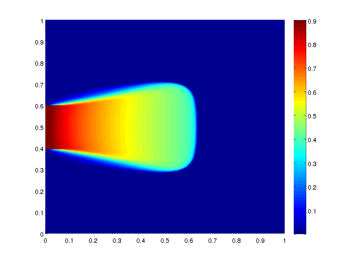
Figure 4: A comparison of the TP-model (49) for γ{1,14,18,116,132}𝛾11418116132\gamma\in\{1,\frac{1}{4},\frac{1}{8},\frac{1}{16},\frac{1}{32}\} with the VE-model (66) using M=5𝑀5M=5 and T=0.3𝑇0.3T=0.3.

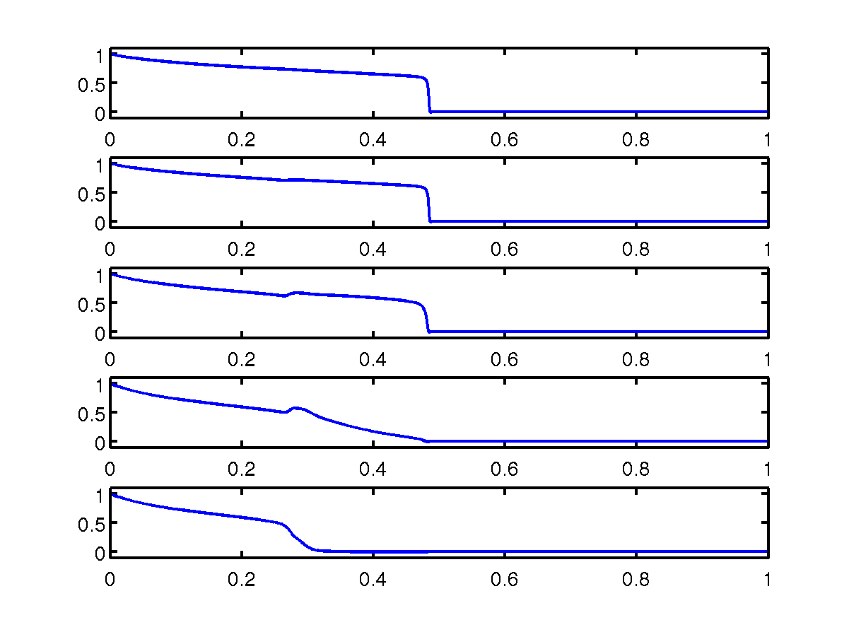
Example 1: We consider the TP-model (49) in five domains Ωv,L=(0,L)×(0,1),L{1,4,8,16,32}formulae-sequencesubscriptΩ𝑣𝐿0𝐿01𝐿1481632\Omega_{v,L}=(0,L)\times(0,1),~{}L\in\{1,4,8,16,32\}. Figures 4(a) - 4(e) present the numerical solutions of the TP-model (49) using the IMPES-method (implicit pressure - explicit saturation) HuberHelmig1999 with pressure p=1𝑝1p=1 at the inflow boundary and p=0𝑝0p=0 at the outflow boundary. In Figure 4(f) the numerical solution of the VE-model (66) is displayed, using the finite-volume scheme (68)-(71). The numerical solutions in Figure 4 correspond to a uniform Cartesian grid of 200×200200200200\times 200 elements in the dimensionless domain D𝐷D.

Grid size Nx×Nzsubscript𝑁𝑥subscript𝑁𝑧N_{x}\times N_{z} 100×100100100100\times 100 200×200200200200\times 200 400×400400400400\times 400
VE-model 0.94 s 10 s 124.51 s
TP-model 6.7 s 64.5 s 722.79 s
Table 1: CPU-time for solving the VE-model compared to the CPU-time for solving the TP-model

.

Figure 4 shows that numerical solutions of the TP-model (49) converge to the corresponding numerical solution of the VE-model, as the domain parameter γ=(1/L)𝛾1𝐿\gamma=(1/L) tends to 00. Moreover, the VE-model describes the vertical dynamics in the medium and, consequently, the spreading speed of the invading front is captured well. These observations indicate that the VE-model is a proper reduction of the two-phase flow model for asymptotically flat domains.

Example 2: Let the dimensionless domain D𝐷D be discretized into a uniform Cartesian grid with equal numbers of vertical and horizontal cells Nz=Nxsubscript𝑁𝑧subscript𝑁𝑥N_{z}=N_{x}. Set γ=1/60𝛾160\gamma=1/60 in the TP-model (49), T=0.3𝑇0.3T=0.3 and M=5𝑀5M=5. In Table 1, we present the CPU-time required by the TP-model model using the IMPES-method and the VE-model using the finite-volume scheme in Section 3.1.

The data from Table 1 shows that the computational time required to solve the VE-model is almost six times less than for the TP-model (49). This is a consequence of solving an algebraic system that results from discretizing the two-dimensional elliptic equation of pressure in the two-phase flow model (49). The performance of the elliptic solver could of course be optimized. This would improve the results for the TP-model, but not change the overall result.

Example 3: The comparison in Example 2 is repeated with a fixed number of vertical cells, but varying the number of horizontal cells Nx=iNz,i{0.5, 1, 2, 4, 8}formulae-sequencesubscript𝑁𝑥𝑖subscript𝑁𝑧𝑖0.51248N_{x}=iN_{z},\,i\in\{0.5,\,1,\,2,\,4,\,8\}. This scenario fits to the case of asymptotically flat domains.

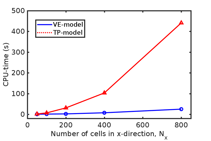
From Table 2 we see that the computational time required for solving the VE-model is almost ten times less than for the TP-model, when Nx=2×Nzsubscript𝑁𝑥2subscript𝑁𝑧N_{x}=2\times N_{z}. However, in the case Nx=16×Nzsubscript𝑁𝑥16subscript𝑁𝑧N_{x}=16\times N_{z}, the computational time required for solving the VE-model is almost 181818 times less than for the TP-model.

Grid size Nx×Nzsubscript𝑁𝑥subscript𝑁𝑧N_{x}\times N_{z} VE-model TP-model
50×1005010050\times 100 0.35 s 1.5 s
100×100100100100\times 100 0.94 s 6.7 s
200×100200100200\times 100 1.9 s 30.8 s
400×100400100400\times 100 7.3 s 103 s
800×100800100800\times 100 25 s 441 s
Table 2: CPU-time for solving the VE-model compared to that for solving the TP-model such that Nx=iNz,i{0.5, 1, 2, 4, 8}formulae-sequencesubscript𝑁𝑥𝑖subscript𝑁𝑧𝑖0.51248N_{x}=iN_{z},\,i\in\{0.5,\,1,\,2,\,4,\,8\}.

This example shows that increasing the number of horizontal cells Nxsubscript𝑁𝑥N_{x}, while keeping Nzsubscript𝑁𝑧N_{z} fixed, limitedly increases the computational time for solving the VE-model as illustrated in Figure 5. On the contrary, the computational time for solving the TP-model significantly increases as the dimension of the algebraic system, resulting from applying the finite difference method to the elliptic equation of pressure, grows.

The numerical examples in this section show the validity of the VE-model in asymptotically flat domains. In addition, they demonstrate a significant reduction in computational complexity of the VE-model, mainly when using grids that are finer in the horizontal than in the vertical direction.
Refer to caption
Figure 5: CPU-time for grids with fixed Nz=100subscript𝑁𝑧100N_{z}=100 and varying Nx{50, 100, 200, 400, 800}subscript𝑁𝑥50100200400800N_{x}\in\{50,\,100,\,200,\,400,\,800\}.

3.3 VE-Model vs. VI-Model

This section highlights the property of describing vertical dynamics by the VE-model and its effect on well-estimating the spreading speed. Different numerical examples that link the VE-model (66) with the VI-model (19) are performed.

In a vertical cross-section ΩvsubscriptΩ𝑣\Omega_{v} of Ω3Ωsuperscript3\Omega\subset\mathbb{R}^{3}, the VI-model (19) reduces to a one-dimensional equation. Using dimensionless variables it is given by

tS+zf(S)=0 in (0,1)×(0,T).subscript𝑡𝑆subscript𝑧𝑓𝑆0 in 010𝑇\displaystyle\partial_{t}S+\partial_{z}f(S)=0\quad\quad\text{ in }(0,1)\times(0,T). (73)

We establish a comparison between the VI-model (73) and the VE-model (66) such that the two-dimensional domain D=(0,1)×(0,1)𝐷0101D=(0,1)\times(0,1) consists of a set of adjacent horizontal layers as in Figure 6. This reduces the VE-model to a coupled system of one-dimensional equations, each of them describing the dynamics in the corresponding layer and taking into account the mass vertical exchange between adjacent layers. Then, the number of vertical cells Nzsubscript𝑁𝑧N_{z} in the finite-volume scheme (68) equals the number of layers in the domain.

It is easy to check that the VI-model (73) corresponds to the one-layer scenario Nz=1subscript𝑁𝑧1N_{z}=1 in the VE-model. Therefore, the comparison of the VE-model (66) to the VI-model (73) is based on varying the number of layers in the domain: Nz=1subscript𝑁𝑧1N_{z}=1 (the VI-model), Nz=2subscript𝑁𝑧2N_{z}=2, and Nz=5subscript𝑁𝑧5N_{z}=5. The two-dimensional VE-model is used here as a reference for accuracy.

It is clear that the computational complexity of the VE-model with Nz=1subscript𝑁𝑧1N_{z}=1 (the VI-model) is the lowest, and increases with the number of layers. However, the following examples show that decreasing the number of layers to Nz=1subscript𝑁𝑧1N_{z}=1 has a strong impact on overestimating the spreading speed of the invading fluid.

The models’ comparison is based on two examples. In the first example, Sinflowsubscript𝑆inflowS_{\text{inflow}} is independent of z𝑧z, but the permeability κ𝜅\kappa changes along the vertical axis. In the second example, κ𝜅\kappa is z𝑧z-independent but Sinflowsubscript𝑆inflowS_{\text{inflow}} is injected only at the lower part of the inflow boundary. In both examples, we set M=2𝑀2M=2, Nx=1000subscript𝑁𝑥1000N_{x}=1000 and T=0.3𝑇0.3T=0.3.

x𝑥x-directionz𝑧z-direction
Figure 6: A vertical-cross section of a 3D domain consisting of 666 thin layers.

Example 1: We assume constant saturation Sinflow=1subscript𝑆inflow1S_{\text{inflow}}=1 along the inflow boundary. The domain consists of two parts with different permeabilities

κ={1,in Dupper:=(0,1)×(0.5,1),0.5,in Dlower:=(0,1)×(0,0.5).𝜅cases1assignin subscript𝐷upper010.510.5assignin subscript𝐷lower0100.5\displaystyle\kappa=\left\{\begin{array}[]{cc}1,&\text{in }D_{\text{upper}}:=(0,1)\times(0.5,1),\\ 0.5,&\text{in }D_{\text{lower}}:=(0,1)\times(0,0.5).\end{array}\right. (76)

This condition is approximated according to the number of layers, i.e.

κj=1Δz(j1)ΔzjΔzκ(z)𝑑z,j=1,,Nz.formulae-sequencesubscript𝜅𝑗1Δ𝑧superscriptsubscript𝑗1Δ𝑧𝑗Δ𝑧𝜅𝑧differential-d𝑧𝑗1subscript𝑁𝑧\displaystyle\kappa_{j}=\frac{1}{\Delta z}\int_{(j-1)\Delta z}^{j\Delta z}\kappa(z)\,dz,\quad\quad j=1,\cdots,N_{z}. (77)

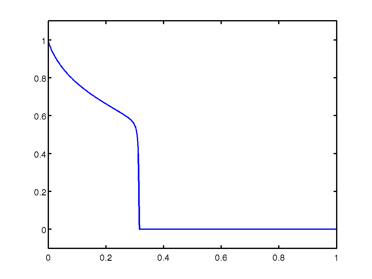
In Figure 7, we show the effect of different permeabilities in the horizontal layers on the models’ accuracy. Figure 7(a) presents the numerical solution of the VI-model (73) with averaged permeability κ=0.75𝜅0.75\kappa=0.75. In Figure 7(b), the domain consists of two layers: the lower layer has low permeability κ1=0.5subscript𝜅10.5\kappa_{1}=0.5 and the upper layer has high permeability κ2=1subscript𝜅21\kappa_{2}=1. In Figure 7(c), the domain consists of five layers. The averaged permeabilities in the layers are: κ1=0.5,κ2=0.5,κ3=0.75,κ4=1formulae-sequencesubscript𝜅10.5formulae-sequencesubscript𝜅20.5formulae-sequencesubscript𝜅30.75subscript𝜅41\kappa_{1}=0.5,\,\kappa_{2}=0.5,\,\kappa_{3}=0.75,\,\kappa_{4}=1 and κ5=1subscript𝜅51\kappa_{5}=1, respectively from bottom to top. Figure 7(d) represents the numerical solution of the VE-model (66) using vertical step size Δz=0.01Δ𝑧0.01\Delta z=0.01.

Refer to caption
(a) VI model (73)
Refer to caption
(b) VE-model (66) with Nz=2subscript𝑁𝑧2N_{z}=2
Refer to caption
(c) VE-model (66) with Nz=5subscript𝑁𝑧5N_{z}=5
Refer to caption
(d) VE-model (66) with Nz=100subscript𝑁𝑧100N_{z}=100
Figure 7: A comparison of the VI-model (73) to the VE-model (66) for κ𝜅\kappa as in (76), Sinflow=1subscript𝑆inflow1S_{\text{inflow}}=1, M=2𝑀2M=2, T=0.3𝑇0.3T=0.3 and Δx=0.001Δ𝑥0.001\Delta x=0.001.

To sum up, Figure 7 shows that the spreading speed of the invading fluid is overestimated by the VI-model (73), compared to the reference solution in Figure 7(d). On the contrary, the spreading speed and the saturation distribution of the VE-model with Nz=2subscript𝑁𝑧2N_{z}=2 and Nz=5subscript𝑁𝑧5N_{z}=5 are well captured. This result is not limited to this example, but expected to hold for other cases where permeability changes along the vertical dimension of the medium.

Example 2: We consider a domain with homogeneous permeability κ=1𝜅1\kappa=1, such that the invading fluid is injected only at the lower part of the inflow boundary, i.e.

Sinflow(z)={1,0z0.2,0,0.2z1.subscript𝑆inflow𝑧cases10𝑧0.200.2𝑧1\displaystyle S_{\text{inflow}}(z)=\left\{\begin{array}[]{c c}1,&0\leq z\leq 0.2,\\ 0,&0.2\leq z\leq 1.\end{array}\right. (80)

This condition is discretized according to the number of layers Nzsubscript𝑁𝑧N_{z} in the domain, i.e.

Sinflow,j=1Δz(j1)ΔzjΔzSinflow(z)𝑑z,j=1,,Nz.formulae-sequencesubscript𝑆inflow𝑗1Δ𝑧superscriptsubscript𝑗1Δ𝑧𝑗Δ𝑧subscript𝑆inflow𝑧differential-d𝑧𝑗1subscript𝑁𝑧\displaystyle S_{\text{inflow},j}=\frac{1}{\Delta z}\int_{(j-1)\Delta z}^{j\Delta z}S_{\text{inflow}}(z)\,dz,\quad\quad j=1,\cdots,N_{z}. (81)

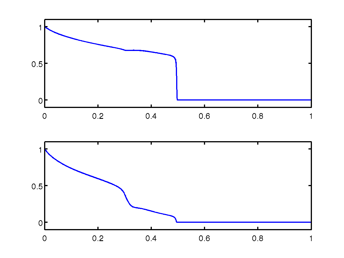
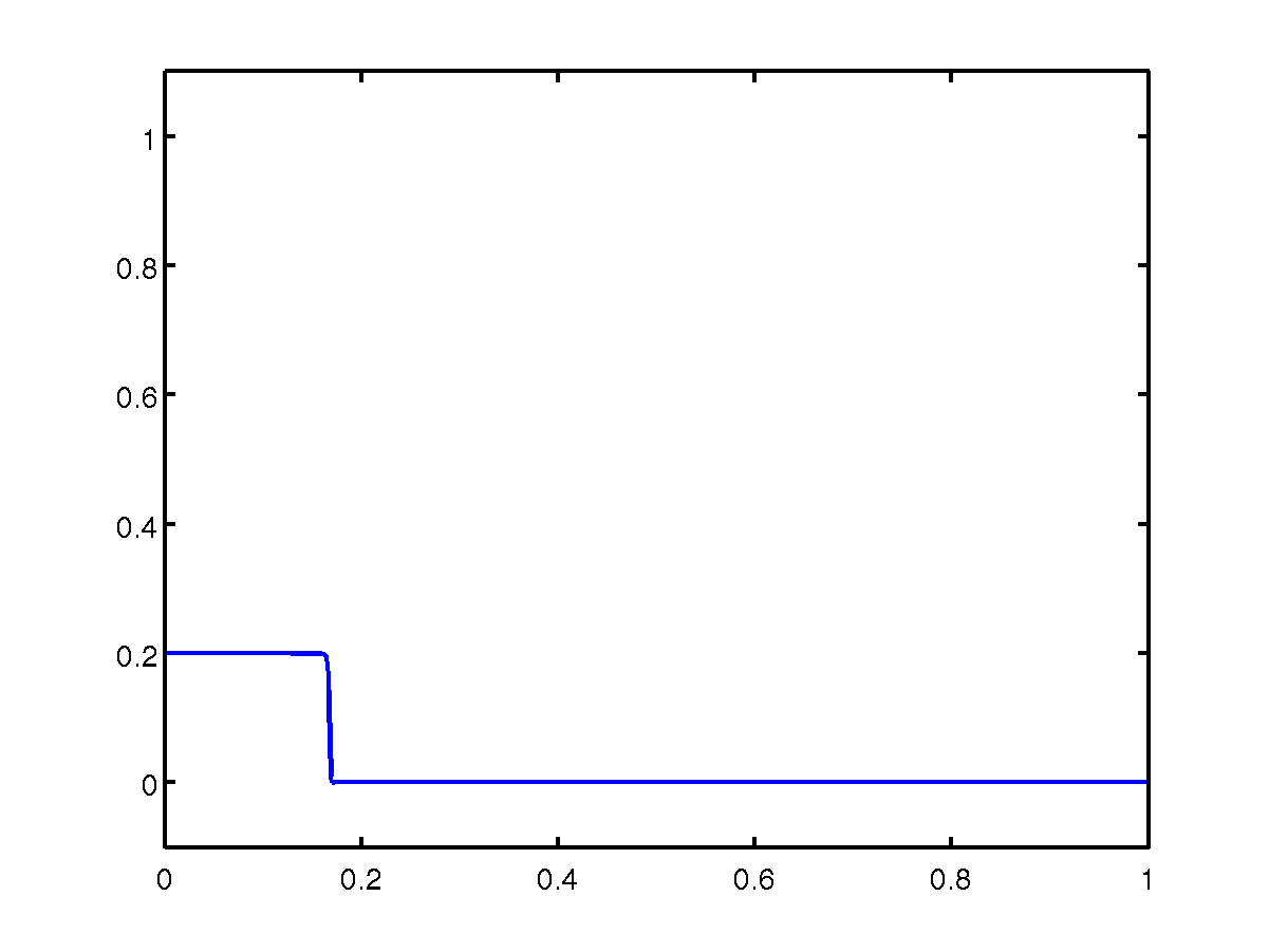
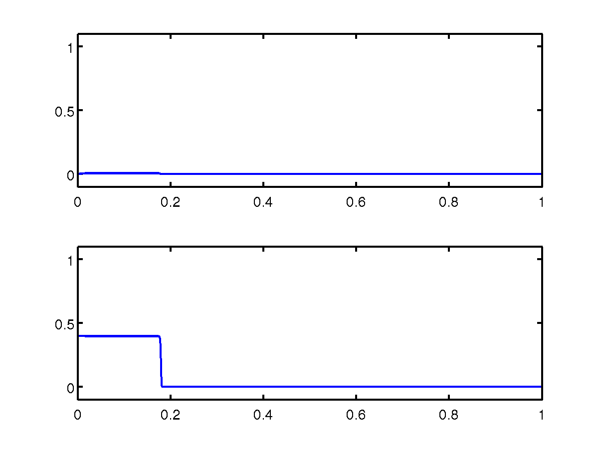
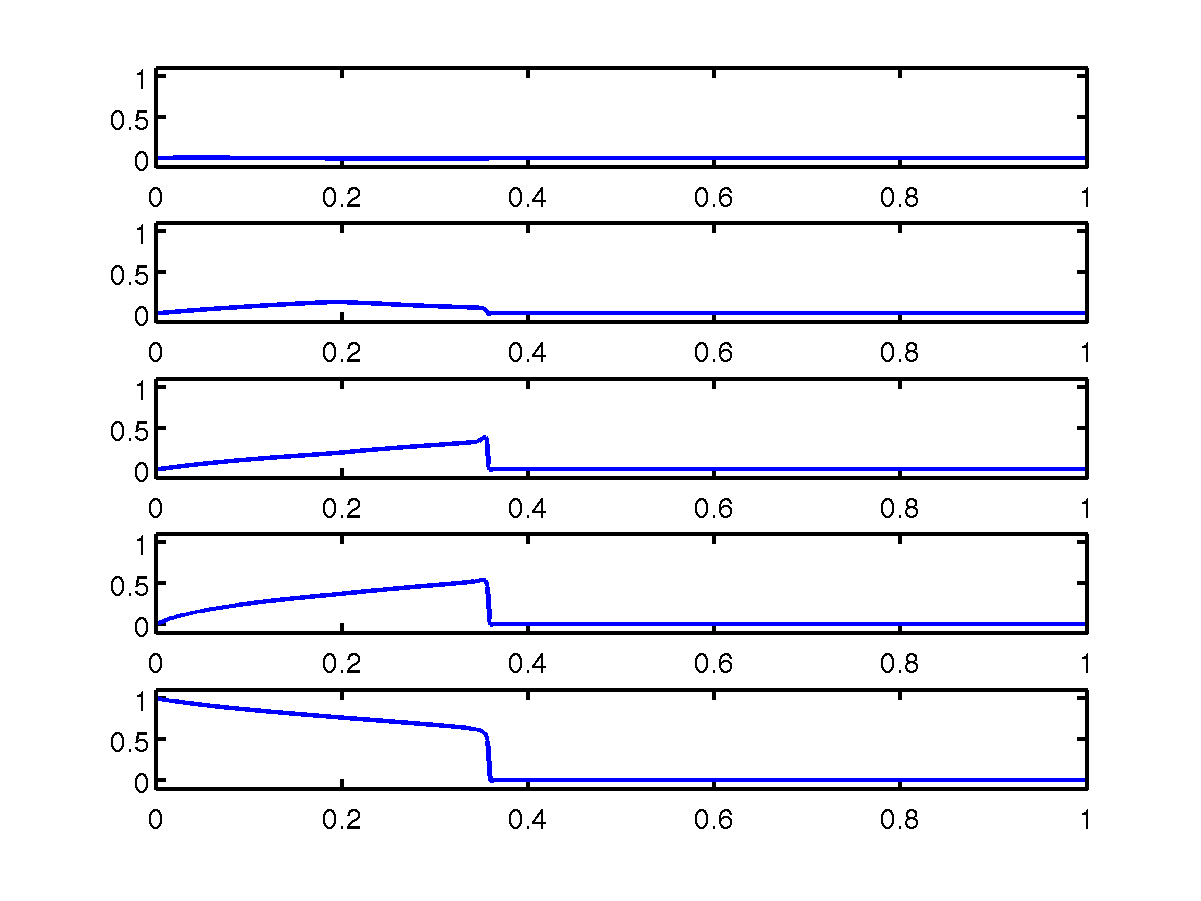
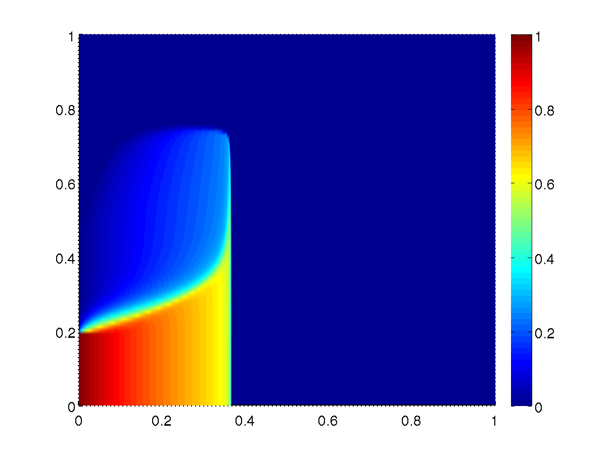
In Figure 8(a), we show the numerical solution of the VI-model (73) with averaged inflow Sinflow=0.2subscript𝑆inflow0.2S_{\text{inflow}}=0.2. Figure 8(b) provides the numerical solution of the VE-model with Nz=2subscript𝑁𝑧2N_{z}=2 such that Sinflow,1=0.4subscript𝑆inflow10.4S_{\text{inflow},1}=0.4 in the lower layer and Sinflow,2=0subscript𝑆inflow20S_{\text{inflow},2}=0 in the upper one. The numerical solution of the VE-model with Nz=5subscript𝑁𝑧5N_{z}=5 is presented in Figure 8(c) such that Sinflow,1=1,Sinflow,2=0,Sinflow,3=0,Sinflow,4=0formulae-sequencesubscript𝑆inflow11formulae-sequencesubscript𝑆inflow20formulae-sequencesubscript𝑆inflow30subscript𝑆inflow40S_{\text{inflow},1}=1,\,S_{\text{inflow},2}=0,\,S_{\text{inflow},3}=0,\,S_{\text{inflow},4}=0 and Sinflow,5=0subscript𝑆inflow50S_{\text{inflow},5}=0 from bottom to top. Finally, the numerical solution of the VE-model (66) with Δz=0.01Δ𝑧0.01\Delta z=0.01 is given in Figure 8(d) as a reference for accuracy.

This example emphasizes the weakness of the VI-model (73) whenever the fluid’s injection position depends on the z𝑧z-coordinate of the domain. In contrast to Example 2, the two-layers case Nz=2subscript𝑁𝑧2N_{z}=2 in the VE-model is not sufficient to give a good estimation of the spreading speed. However, the spreading speed and the fluids’ distribution in the five-layers case Nz=5subscript𝑁𝑧5N_{z}=5 are in excellent agreement with the reference solution in Figure 8(d).

Example 1 and Example 2 show the impact of varying the vertical permeability and the injection position on overestimating the spreading speed using the VI-model. On the contrary, the VE-model provides better estimates even using a very small number of vertical cells.

Refer to caption
(a) VI-model (73)
Refer to caption
(b) VE-model (66) with N=2𝑁2N=2
Refer to caption
(c) VE-model (66) with N=5𝑁5N=5
Refer to caption
(d) VE-model (66) with N=100𝑁100N=100
Figure 8: A comparison of the VI-model (73) with the VE-model (66) for Sinflowsubscript𝑆inflowS_{\text{inflow}} as in (80), κ=1𝜅1\kappa=1, M=2𝑀2M=2, T=0.3𝑇0.3T=0.3 and Δx=0.001Δ𝑥0.001\Delta x=0.001.

3.4 VE-Model vs. Multiscale Model

Under the same conditions assumed to derive the VE-model (66), we prove in this section that the Multiscale model (24), (31) and (32) in the vertical cross-section Ωv=(0,1)×(0,1)subscriptΩ𝑣0101\Omega_{v}=(0,1)\times(0,1) is equivalent to the VE-model. For the sake of simplicity, we also assume negligible gravity and capillary forces. Then, using the dimensionless variables (39), the Multiscale model (24), (31) reduces to

x(λ^tot(S^α)κ^xp^)=0 in (0,1)×(0,T),subscript𝑥subscript^𝜆𝑡𝑜𝑡subscript^𝑆𝛼^𝜅subscript𝑥^𝑝0 in 010𝑇\displaystyle-\partial_{x}\bigl{(}\hat{\lambda}_{tot}(\hat{S}_{\alpha})\hat{\kappa}\partial_{x}\hat{p}\bigr{)}=0\quad\quad\text{ in }(0,1)\times(0,T), (82)

and in D×(0,T)𝐷0𝑇D\times(0,T)

p(x,z,t)=p^(x,t),λtot(Sα)κ1xp=u,zw=xu,ϕtSα+x(uf(Sα))+z(wf(Sα))=0.𝑝𝑥𝑧𝑡absent^𝑝𝑥𝑡subscript𝜆𝑡𝑜𝑡subscript𝑆𝛼subscript𝜅1subscript𝑥𝑝absent𝑢subscript𝑧𝑤absentsubscript𝑥𝑢italic-ϕsubscript𝑡subscript𝑆𝛼subscript𝑥𝑢𝑓subscript𝑆𝛼subscript𝑧𝑤𝑓subscript𝑆𝛼absent0\displaystyle\begin{array}[]{rl}p(x,z,t)=&\,\hat{p}(x,t),\\ -\lambda_{tot}(S_{\alpha})\kappa_{1}\partial_{x}p=&u,\\ \partial_{z}w=&-\partial_{x}u,\\ \phi\partial_{t}S_{\alpha}+\partial_{x}\big{(}uf(S_{\alpha})\big{)}+\partial_{z}\big{(}wf(S_{\alpha})\big{)}=&\,0.\end{array} (87)

Note here that the assumption of negligible gravity and capillary forces implies that πα=0subscript𝜋𝛼0\pi_{\alpha}=0 (see (32)). This model is closed with the initial and boundary conditions

S^α=S^0, in (0,1),S^α=S^inflow, on {0}×[0,T],Sα=S0, in D,Sα=Sinflow, on Dinflow×[0,T],nvα=0, on Dimp×[0,T].subscript^𝑆𝛼absentsubscript^𝑆0 in 01subscript^𝑆𝛼absentsubscript^𝑆inflow on 00𝑇subscript𝑆𝛼absentsubscript𝑆0 in 𝐷subscript𝑆𝛼absentsubscript𝑆inflow on subscript𝐷inflow0𝑇nsubscriptv𝛼absent0 on subscript𝐷imp0𝑇\displaystyle\begin{array}[]{rll}\hat{S}_{\alpha}&=\hat{S}_{0},&\text{ in }(0,1),\\ \hat{S}_{\alpha}&=\hat{S}_{\text{inflow}},&\text{ on }\{0\}\times[0,T],\\ S_{\alpha}&=S_{0},&\text{ in }D,\\ S_{\alpha}&=S_{\text{inflow}},&\text{ on }\partial D_{\text{inflow}}\times[0,T],\\ \textbf{n}\cdot\textbf{v}_{\alpha}&=0,&\text{ on }\partial D_{\text{imp}}\times[0,T].\end{array} (93)
Theorem 3.1

For T>0𝑇0T>0, let (SM,uM,wM,p^M)subscript𝑆𝑀subscript𝑢𝑀subscript𝑤𝑀subscript^𝑝𝑀(S_{M},u_{M},w_{M},\hat{p}_{M}) be a smooth solution of the Multiscale model (82), (87) in D×(0,T)𝐷0𝑇D\times(0,T) with the initial and boundary conditions (93). For T¯:=0Th(r)𝑑r+h(0)Tassign¯𝑇superscriptsubscript0𝑇𝑟differential-d𝑟0𝑇\overline{T}:=\int_{0}^{T}h(r)dr+h(0)T, where h(t)=01uM(0,z,t)𝑑z𝑡superscriptsubscript01subscript𝑢𝑀0𝑧𝑡differential-d𝑧h(t)=\int_{0}^{1}u_{M}(0,z,t)\,dz, let (SVE,uVE,wVE)subscript𝑆𝑉𝐸subscript𝑢𝑉𝐸subscript𝑤𝑉𝐸(S_{VE},u_{VE},w_{VE}) be a smooth solution of the VE-model (66) in D×(0,T¯)𝐷0¯𝑇D\times(0,\overline{T}) with the initial and boundary conditions (10). Then, SM(,,t)=SVE(,,t¯),uM(,,t)=uVE(,,t¯)formulae-sequencesubscript𝑆𝑀𝑡subscript𝑆𝑉𝐸¯𝑡subscript𝑢𝑀𝑡subscript𝑢𝑉𝐸¯𝑡S_{M}(\cdot,\cdot,t)=S_{VE}(\cdot,\cdot,\bar{t}),\,u_{M}(\cdot,\cdot,t)=u_{VE}(\cdot,\cdot,\bar{t}) and wM(,,t)=wVE(,,t¯)subscript𝑤𝑀𝑡subscript𝑤𝑉𝐸¯𝑡w_{M}(\cdot,\cdot,t)=w_{VE}(\cdot,\cdot,\bar{t}) in D𝐷D where t¯:=0th(r)𝑑r+h(0)tassign¯𝑡superscriptsubscript0𝑡𝑟differential-d𝑟0𝑡\overline{t}:=\int_{0}^{t}h(r)dr+h(0)t for any t(0,T)𝑡0𝑇t\in(0,T). Furthermore, there is a function pVE=pVE(SVE)subscript𝑝𝑉𝐸subscript𝑝𝑉𝐸subscript𝑆𝑉𝐸p_{VE}=p_{VE}(S_{VE}) with

xpVE(x,t)=101κ(x,z)λtot(SVE(x,z,t))𝑑zsubscript𝑥subscript𝑝𝑉𝐸𝑥𝑡1superscriptsubscript01𝜅𝑥𝑧subscript𝜆𝑡𝑜𝑡subscript𝑆𝑉𝐸𝑥𝑧𝑡differential-d𝑧\displaystyle\partial_{x}p_{VE}(x,t)=\frac{1}{\int_{0}^{1}\kappa(x,z)\lambda_{tot}\big{(}S_{VE}(x,z,t)\big{)}\,dz}

and p^M(,t)=pVE(,t¯)subscript^𝑝𝑀𝑡subscript𝑝𝑉𝐸¯𝑡\hat{p}_{M}(\cdot,t)=p_{VE}(\cdot,\bar{t}) in (0,1)01(0,1).

In view of the equivalence result of Theorem 3.1, the finite-volume scheme in Section 3.1 is also applicable for the Multiscale model (82), (87). This leads to a reduced computational complexity of the Multiscale model compared with that using a multiscale algorithm proposed in Guo2014 . This algorithm is analogous to the IMPES-method with an implicit treatment for the pressure at the coarse scale and an explicit treatment for the saturation at the fine scale.

Proof

Let (SM,uM,wM,p^M)subscript𝑆𝑀subscript𝑢𝑀subscript𝑤𝑀subscript^𝑝𝑀(S_{M},u_{M},w_{M},\hat{p}_{M}) be a smooth solution of the Multiscale model (82), (87). Then, the coarse-scale equation (82) implies that the vertically averaged horizontal velocity,

u^M=λ^tot(S^M)κ^xp^M,subscript^𝑢𝑀subscript^𝜆𝑡𝑜𝑡subscript^𝑆𝑀^𝜅subscript𝑥subscript^𝑝𝑀\displaystyle\hat{u}_{M}=-\hat{\lambda}_{tot}(\hat{S}_{M})\hat{\kappa}\partial_{x}\hat{p}_{M}, (94)

satisfies

xu^M=0.subscript𝑥subscript^𝑢𝑀0\displaystyle\partial_{x}\hat{u}_{M}=0. (95)

Integrating (95) over the x𝑥x-direction from 00 to an arbitrary x(0,1)𝑥01x\in(0,1) yields

u^M(x,t)hM(t)=0,subscript^𝑢𝑀𝑥𝑡subscript𝑀𝑡0\displaystyle\hat{u}_{M}(x,t)-h_{M}(t)=0, (96)

where hM(t)=u^M(0,t)subscript𝑀𝑡subscript^𝑢𝑀0𝑡h_{M}(t)=\hat{u}_{M}(0,t) is the averaged horizontal velocity at the inflow boundary Dinflowsubscript𝐷inflow\partial D_{\text{inflow}} with hM(t)>0subscript𝑀𝑡0h_{M}(t)>0 for all t[0,T]𝑡0𝑇t\in[0,T]. Substituting (96) into (94) and noting that the vertically-averaged quantities κ^^𝜅\hat{\kappa} and λ^totsubscript^𝜆𝑡𝑜𝑡\hat{\lambda}_{tot} are defined as in (14), we obtain that

xp^M(x,t)=hM(t)01κ(x,z)λtot(SM(x,z,t))𝑑z,subscript𝑥subscript^𝑝𝑀𝑥𝑡subscript𝑀𝑡superscriptsubscript01𝜅𝑥𝑧subscript𝜆𝑡𝑜𝑡subscript𝑆𝑀𝑥𝑧𝑡differential-d𝑧\displaystyle\partial_{x}\hat{p}_{M}(x,t)=\frac{h_{M}(t)}{\int_{0}^{1}\kappa(x,z)\lambda_{tot}(S_{M}(x,z,t))\,dz}, (97)

which coincides with the definition of xpVExp0subscript𝑥subscript𝑝𝑉𝐸subscript𝑥subscript𝑝0\partial_{x}p_{VE}\coloneqq\partial_{x}p_{0} in equation (65). Using the first equation in the fine-scale model (87), we obtain that

xpM(x,z,t)=hM(t)01κ(x,z)λtot(Sα(x,z,t))𝑑z,subscript𝑥subscript𝑝𝑀𝑥𝑧𝑡subscript𝑀𝑡superscriptsubscript01𝜅𝑥𝑧subscript𝜆𝑡𝑜𝑡subscript𝑆𝛼𝑥𝑧𝑡differential-d𝑧\displaystyle\partial_{x}p_{M}(x,z,t)=\frac{h_{M}(t)}{\int_{0}^{1}\kappa(x,z)\lambda_{tot}(S_{\alpha}(x,z,t))\,dz}, (98)

which is in fact independent of the vertical coordinate z𝑧z as the reconstruction operator πisubscript𝜋𝑖\pi_{i} in this setting equals zero. Substituting equation (98) into the second equation in (87) yields the horizontal velocity uMsubscript𝑢𝑀u_{M} as an expression of saturation alone

uM[x,z,t;SM]=hM(t)κ(x,z)λtot(SM(x,z,t))01κ(x,z)λtot(SM(x,z,t))𝑑z.subscript𝑢𝑀𝑥𝑧𝑡subscript𝑆𝑀subscript𝑀𝑡𝜅𝑥𝑧subscript𝜆𝑡𝑜𝑡subscript𝑆𝑀𝑥𝑧𝑡superscriptsubscript01𝜅𝑥𝑧subscript𝜆𝑡𝑜𝑡subscript𝑆𝑀𝑥𝑧𝑡differential-d𝑧\displaystyle u_{M}[x,z,t;S_{M}]=-\frac{h_{M}(t)\kappa(x,z)\lambda_{tot}\big{(}S_{M}(x,z,t)\big{)}}{\int_{0}^{1}\kappa(x,z)\lambda_{tot}\big{(}S_{M}(x,z,t)\big{)}\,dz}. (99)

Substituting (99) into the third equation in (87) then integrating over the vertical coordinate from 00 to an arbitrary z(0,1)𝑧01z\in(0,1) yields the vertical velocity as an expression of saturation alone

wM[x,z,t;SM]=subscript𝑤𝑀𝑥𝑧𝑡subscript𝑆𝑀absent\displaystyle w_{M}[x,z,t;S_{M}]= x0zuM[x,r,t;SM]𝑑r.subscript𝑥superscriptsubscript0𝑧subscript𝑢𝑀𝑥𝑟𝑡subscript𝑆𝑀differential-d𝑟\displaystyle-\partial_{x}\int_{0}^{z}u_{M}[x,r,t;S_{M}]\,dr. (100)

We substitute equation (99) and (100) into the fourth equation in the fine-scale model (87), then rescale the time using tt¯=0thM(r)𝑑r+hM(0)tmaps-to𝑡¯𝑡superscriptsubscript0𝑡subscript𝑀𝑟differential-d𝑟subscript𝑀0𝑡t\mapsto\bar{t}=\int_{0}^{t}h_{M}(r)dr+h_{M}(0)t. As a result, the Multiscale model simplifies to

tSM+x(uM[,;\displaystyle\partial_{t}S_{M}+\partial_{x}\big{(}u_{M}[\cdot,\cdot; SM]f(SM))+z(w[,;SM]f(SM))=0,\displaystyle S_{M}]f(S_{M})\big{)}+~{}\partial_{z}\big{(}w[\cdot,\cdot;S_{M}]~{}f(S_{M})\big{)}=0,
uM[,;SM]subscript𝑢𝑀subscript𝑆𝑀\displaystyle u_{M}[\cdot,\cdot;S_{M}] =λtot(SM)κ01λtot(SM(,z,))κ(,z)𝑑z,absentsubscript𝜆𝑡𝑜𝑡subscript𝑆𝑀𝜅superscriptsubscript01subscript𝜆𝑡𝑜𝑡subscript𝑆𝑀𝑧𝜅𝑧differential-d𝑧\displaystyle=\dfrac{\lambda_{tot}(S_{M})\kappa}{\int_{0}^{1}\lambda_{tot}\big{(}S_{M}(\cdot,z,\cdot)\big{)}\kappa(\cdot,z)\,dz},
wM[,z;SM(,z,)]subscript𝑤𝑀𝑧subscript𝑆𝑀𝑧\displaystyle w_{M}[\cdot,z;S_{M}(\cdot,z,\cdot)] =x0zλtot(SM(,r,))κ(,r)𝑑r01λtot(SM(,r,))κ(,r)𝑑r,absentsubscript𝑥superscriptsubscript0𝑧subscript𝜆𝑡𝑜𝑡subscript𝑆𝑀𝑟𝜅𝑟differential-d𝑟superscriptsubscript01subscript𝜆𝑡𝑜𝑡subscript𝑆𝑀𝑟𝜅𝑟differential-d𝑟\displaystyle=-\partial_{x}\dfrac{\int_{0}^{z}\lambda_{tot}\big{(}S_{M}(\cdot,r,\cdot)\big{)}\kappa(\cdot,r)\,dr}{\int_{0}^{1}\lambda_{tot}\big{(}S_{M}(\cdot,r,\cdot)\big{)}\kappa(\cdot,r)\,dr}, (101)

for all z(0,1)𝑧01z\in(0,1), in D×(0,T¯)𝐷0¯𝑇D\times(0,\overline{T}). Note that this scaled time interval coincides with that in the VE-model as the function hMsubscript𝑀h_{M} is equivalent to hVEsubscript𝑉𝐸h_{VE}, defined as in (64).

The simplified version of the Multiscale model (101) requires initial and boundary conditions with respect to the unknown SMsubscript𝑆𝑀S_{M} only. Hence, it is closed with the initial and boundary conditions

SM=S0, in D,SM=Sinflow, on Dinflow×[0,T],nvM=0, on Dimp×[0,T].subscript𝑆𝑀absentsubscript𝑆0 in 𝐷subscript𝑆𝑀absentsubscript𝑆inflow on subscript𝐷inflow0𝑇nsubscriptv𝑀absent0 on subscript𝐷imp0𝑇\displaystyle\begin{array}[]{rll}S_{M}&=S_{0},&\text{ in }D,\\ S_{M}&=S_{\text{inflow}},&\text{ on }\partial D_{\text{inflow}}\times[0,T],\\ \textbf{n}\cdot\textbf{v}_{M}&=0,&\text{ on }\partial D_{\text{imp}}\times[0,T].\end{array} (105)

Hence, a smooth solution (SM,uM,wM,p^M)subscript𝑆𝑀subscript𝑢𝑀subscript𝑤𝑀subscript^𝑝𝑀(S_{M},u_{M},w_{M},\hat{p}_{M}) of the Multiscale model (82), (87) is also a solution of the VE-model. Proving the other direction follows the same argumentation in reversed order. ∎

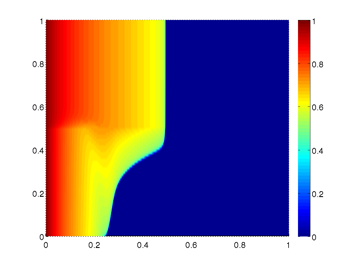
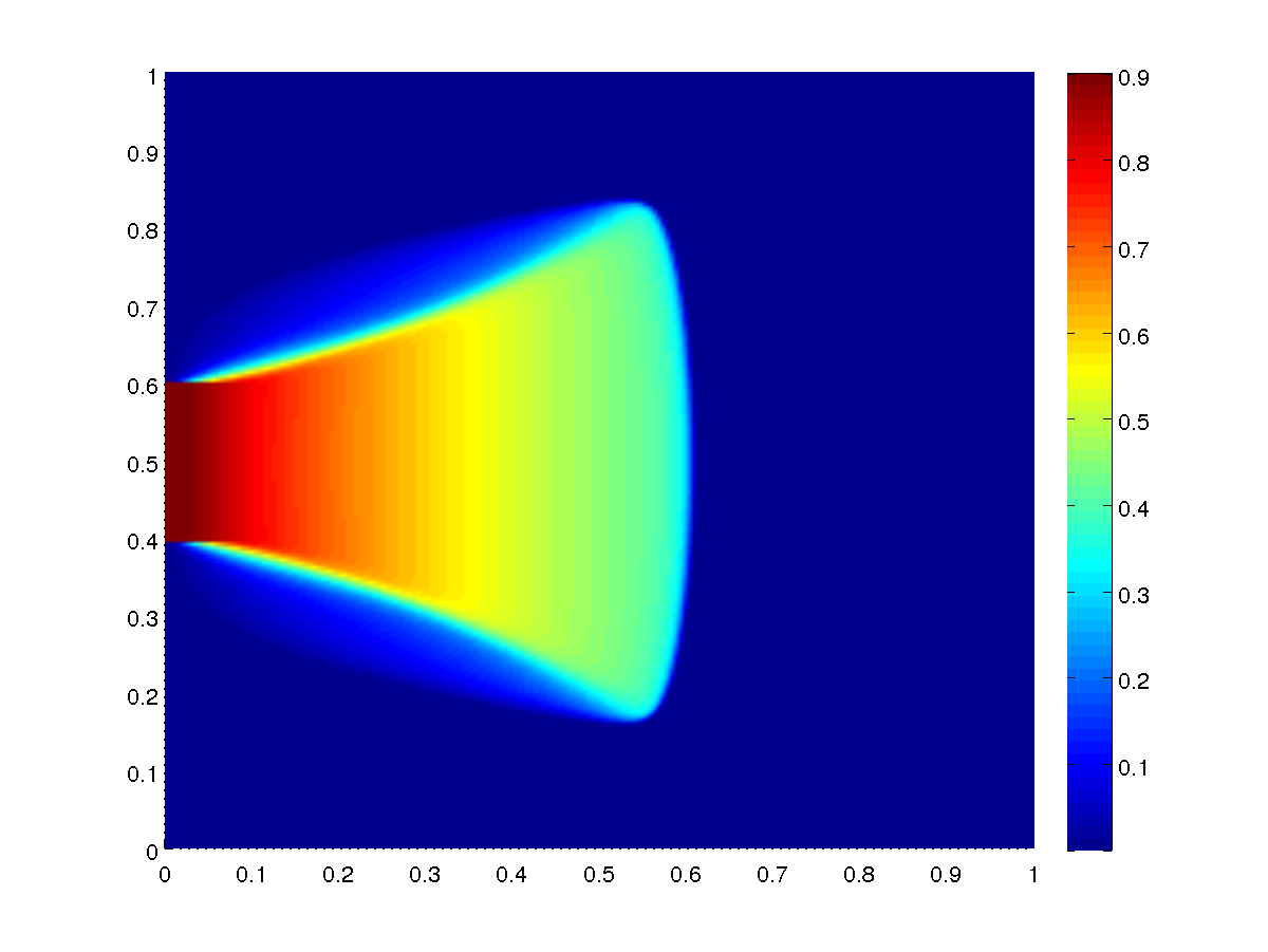
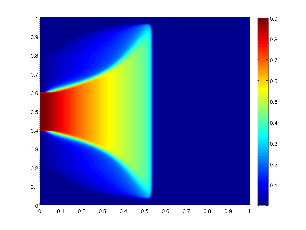
Example 1: Figure 9 compares a numerical solution for the Multiscale model (82), (87) (in the equivalent form of the VE-model) using the finite-volume scheme, presented in Section 3.1, with a numerical solution using the multiscale algorithm in Guo2014 . In both cases, a Cartesian grid with 200×200200200200\times 200 elements is used, the end time is T=0.3𝑇0.3T=0.3 and the viscosity ratio is M=5𝑀5M=5.

Figure 9 displays very similar discrete solutions. This indicates that both schemes have similar accuracy.

Example 2: Table 3 compares the CPU-time for solving the Multiscale model using the finite-volume scheme, presented in Section 3.1, and using the algorithm in Guo2014 . In both cases, Cartesian grids with a fixed number of horizontal cells Nx=100subscript𝑁𝑥100N_{x}=100 and a varying number of vertical cells Nz=iNx,i{1, 2, 4, 8, 16}formulae-sequencesubscript𝑁𝑧𝑖subscript𝑁𝑥𝑖124816N_{z}=iN_{x},\,i\in\{1,\,2,\,4,\,8,\,16\} are used. Table 3 shows that the computational time using the finite-volume scheme is significantly reduced compared to that using the multiscale algorithm, mainly when the horizontal discretization is finer than in vertical one. This results from solving the elliptic equation of the vertically averaged pressure in the Multiscale model, which consumes most of the CPU-time.

Refer to caption
(a) multiscale algorithm
Refer to caption
(b) finite-volume scheme
Figure 9: Numerical solution of the Multiscale model (82), (87) using the multiscale algorithm Guo2014 in (a) and the finite-volume scheme in (b).
Grid size Nx×Nzsubscript𝑁𝑥subscript𝑁𝑧N_{x}\times N_{z} Finite-volume scheme Multiscale algorithm
100×100100100100\times 100 1.08 s 0.91 s
200×100200100200\times 100 2.58 s 2.97 s
400×100400100400\times 100 9 s 12.32 s
800×100800100800\times 100 25 s 64.85 s
1600×10016001001600\times 100 109 s 413 s
Table 3: CPU-time for solving the VE-model using the finite-volume scheme compared to CPU-time for solving the Multiscale model using the multiscale algorithm with T=0.3𝑇0.3T=0.3 and viscosity ratio M=5𝑀5M=5.

Example 3 Using the equivalence result from Theorem 3.1 and following Yortsos Yortsos , we show in this example that the reconstruction function (32) in domains with a small γ𝛾\gamma represents strong gravity effects that lead to a fast segregation of the fluids, meaning that the vertical equilibrium assumption is fully satisfied. This, however, implies that the Multiscale model and the VI-model give results with similar accuracy. Consequently, the VI-model is sufficient to describe the fluids’ flow as it has a lower computational complexity.

We consider the Multiscale model (24), (31) in a vertical cross-section Ωv=(0,L)×(0,H)subscriptΩ𝑣0𝐿0𝐻\Omega_{v}=(0,L)\times(0,H) of Ω3Ωsuperscript3\Omega\subset\mathbb{R}^{3} with negligible capillary forces and using the dimensionless variables (39), that is

x(λ^tot(S^i)κ^xp^)=0 in (0,1)×(0,T),subscript𝑥subscript^𝜆𝑡𝑜𝑡subscript^𝑆𝑖^𝜅subscript𝑥^𝑝0 in 010𝑇\displaystyle-\partial_{x}\bigl{(}\hat{\lambda}_{tot}(\hat{S}_{i})\hat{\kappa}\partial_{x}\hat{p}\bigr{)}=0\quad\text{ in }(0,1)\times(0,T), (106)

and in D×(0,T)𝐷0𝑇D\times(0,T)

p(x,z,t)=p^(x,t)+πi(x,z,t),λtot(Si)κxp=u,1γzw=xu,f(Si)w+gk(ρiρd)γ2q3μdκf(Si)λd(Si)=wi,ϕtSi+x(uf(Si))+1γz(wi)=0.𝑝𝑥𝑧𝑡absent^𝑝𝑥𝑡subscript𝜋𝑖𝑥𝑧𝑡subscript𝜆𝑡𝑜𝑡subscript𝑆𝑖𝜅subscript𝑥𝑝absent𝑢1𝛾subscript𝑧𝑤absentsubscript𝑥𝑢𝑓subscript𝑆𝑖𝑤𝑔𝑘subscript𝜌𝑖subscript𝜌𝑑superscript𝛾2superscript𝑞3subscript𝜇𝑑𝜅𝑓subscript𝑆𝑖subscript𝜆𝑑subscript𝑆𝑖absentsubscript𝑤𝑖italic-ϕsubscript𝑡subscript𝑆𝑖subscript𝑥𝑢𝑓subscript𝑆𝑖1𝛾subscript𝑧subscript𝑤𝑖absent0\displaystyle\begin{array}[]{rl}p(x,z,t)=&\,\hat{p}(x,t)+\pi_{i}(x,z,t),\\ -\lambda_{tot}(S_{i})\kappa\partial_{x}p=&u,\\ \frac{1}{\gamma}\partial_{z}w=&-\partial_{x}u,\\ f(S_{i})w+\frac{gk(\rho_{i}-\rho_{d})}{\gamma^{2}q^{3}\mu_{d}}\kappa f(S_{i})\lambda_{d}(S_{i})=&w_{i},\\ \phi\partial_{t}S_{i}+\partial_{x}\big{(}uf(S_{i})\big{)}+\frac{1}{\gamma}\partial_{z}\big{(}w_{i}\big{)}=&\,0.\\ \end{array} (112)

The dimensionless reconstruction operator is now given as

πi(,z,)=1γqμd0z(Si(,r,)ρi+(1Si(,r,))ρd)g𝑑r,subscript𝜋𝑖𝑧1𝛾𝑞subscript𝜇𝑑superscriptsubscript0𝑧subscript𝑆𝑖𝑟subscript𝜌𝑖1subscript𝑆𝑖𝑟subscript𝜌𝑑𝑔differential-d𝑟\displaystyle\pi_{i}(\cdot,z,\cdot)=-\dfrac{1}{\gamma q\mu_{d}}\int_{0}^{z}\Big{(}S_{i}(\cdot,r,\cdot)\rho_{i}+\big{(}1-S_{i}(\cdot,r,\cdot)\big{)}\rho_{d}\Big{)}g\,dr,

for any z(0,1)𝑧01z\in(0,1).

To prove fluids’ segregation, we consider the fourth equation in (112). With respect to the parameter γ𝛾\gamma, the term on the right side and the first term on the left side are of order 𝒪(1)𝒪1\mathcal{O}(1). However, the second term on the left side is of order 𝒪(γ2)𝒪superscript𝛾2\mathcal{O}(\gamma^{-2}), which diverges as γ𝛾\gamma tends to zero. This leads to a contradiction unless the product fλd𝑓subscript𝜆𝑑f\lambda_{d} satisfies

f(Si)λd(Si)=0,𝑓subscript𝑆𝑖subscript𝜆𝑑subscript𝑆𝑖0\displaystyle f(S_{i})\lambda_{d}(S_{i})=0,

which implies either λd(Si)=0subscript𝜆𝑑subscript𝑆𝑖0\lambda_{d}(S_{i})=0 or f(Si)=0𝑓subscript𝑆𝑖0f(S_{i})=0, i.e. the fluids segregate. Another way to avoid the contradiction in the fourth equation in (112) is to assume a small gravity effect by multiplying the gravity term in the first and the fourth equations in (112) by a small parameter NG=𝒪(γ2)subscript𝑁𝐺𝒪superscript𝛾2N_{G}=\mathcal{O}(\gamma^{2}). By doing this, the second term in the fourth equation in (112) is of order 𝒪(1)𝒪1\mathcal{O}(1). However, the gravity term in the first equation is of order 𝒪(γ)𝒪𝛾\mathcal{O}(\gamma). Therefore, this term can be neglected in media with a small parameter γ𝛾\gamma.

4 Models for Two-Phase Brinkman Flow in Flat Domains

In this part of the paper, we study two-phase flow in flat domains for Brinkman regimes. Examples of such regimes are media with high porosity. First, we present the main governing equations of the Brinkman two-phase flow model. Then, we derive a reduced model that describes two-phase Brinkman flow in flat domains.

4.1 The Brinkman Two-Phase Flow Model (BTP-Model)

Brinkman’s equations describe the flow of incompressible fluids through a porous medium with high porosity Brinkman1949 . Mathematically speaking, the Brinkman equations

(μeΔuα+uαμeΔwα+wα)=krαμαK(pαραg),subscript𝜇𝑒Δsubscript𝑢𝛼subscript𝑢𝛼subscript𝜇𝑒Δsubscript𝑤𝛼subscript𝑤𝛼subscript𝑘𝑟𝛼subscript𝜇𝛼Ksubscript𝑝𝛼subscript𝜌𝛼g\left(\begin{array}[]{c}-\mu_{e}\Delta u_{\alpha}+u_{\alpha}\\ -\mu_{e}\Delta w_{\alpha}+w_{\alpha}\end{array}\right)=-\dfrac{k_{r\alpha}}{\mu_{\alpha}}\textbf{K}(\nabla p_{\alpha}-\rho_{\alpha}\textbf{g}), (113)

are a regularization of Darcy’s law. The terms uαsubscript𝑢𝛼u_{\alpha} and wαsubscript𝑤𝛼w_{\alpha} are the horizontal and vertical components of the velocity vαsubscriptv𝛼\textbf{v}_{\alpha} for the phase α{i,d}𝛼𝑖𝑑\alpha\in\{i,d\}, respectively. The parameter μe>0subscript𝜇𝑒0\mu_{e}>0 is the effective viscosity. The second-order terms Δuα,ΔwαΔsubscript𝑢𝛼Δsubscript𝑤𝛼\Delta u_{\alpha},\ \Delta w_{\alpha} on the left side of (113) correspond to components of the divergence of the stress tensor.

The validity of Brinkman’s equation in porous media has been investigated by many researchers, see Auriault2009 ; Auriault2005 and the references therein. In media with high porosity, the effective viscosity μesubscript𝜇𝑒\mu_{e} is close to the dynamical viscosity. However, if the medium is macroscopiclly nonhomogeneous, the effective viscosity is very small (μe1much-less-thansubscript𝜇𝑒1\mu_{e}\ll 1), such that the second order term in (113) is considered as a corrector of Darcy’s law Auriault2005 . In addition, in porous media with almost unidirectional fluid flows, Brinkman’s equations can be derived by averaging the Navier-Stokes equations over a representative averaging volume Hornung .

We define the vector VαsubscriptV𝛼\textbf{V}_{\alpha}, such that

Vα=(UαWα)(μeΔuα+uαμeΔwα+wα),subscriptV𝛼subscript𝑈𝛼subscript𝑊𝛼subscript𝜇𝑒Δsubscript𝑢𝛼subscript𝑢𝛼subscript𝜇𝑒Δsubscript𝑤𝛼subscript𝑤𝛼\displaystyle\textbf{V}_{\alpha}=\left(\begin{array}[]{c}U_{\alpha}\vspace{5pt}\\ W_{\alpha}\end{array}\right)\coloneqq\left(\begin{array}[]{c}-\mu_{e}\Delta u_{\alpha}+u_{\alpha}\vspace{5pt}\\ -\mu_{e}\Delta w_{\alpha}+w_{\alpha}\end{array}\right), (118)

for each phase α{i,d}𝛼𝑖𝑑\alpha\in\{i,d\}. For incompressible fluids in a porous medium with the assumption of negligible gravity force, the Brinkman two-phase flow model (BTP-model) is a combination of the continuity equation, Brinkman’s equations, and the incompressibility equation, that is

tSα+vα=0,Vα=krαμαKpα,v=0 in Ω×(0,T),subscript𝑡subscript𝑆𝛼subscriptv𝛼absent0subscriptV𝛼absentsubscript𝑘𝑟𝛼subscript𝜇𝛼Ksubscript𝑝𝛼vabsent0 in Ω0𝑇\displaystyle\begin{array}[]{rl}\partial_{t}S_{\alpha}+\nabla\cdot\textbf{v}_{\alpha}&=0,\\ \textbf{V}_{\alpha}&=-\dfrac{k_{r\alpha}}{\mu_{\alpha}}\textbf{K}\nabla p_{\alpha},\\ \nabla\cdot\textbf{v}&=0\end{array}\quad\quad\text{ in }\Omega\times(0,T), (122)

for both invading and defending fluids α{i,d}𝛼𝑖𝑑\alpha\in\{i,d\}, where Ω(0,L)×(0,H)2Ω0𝐿0𝐻superscript2\Omega\coloneqq(0,L)\times(0,H)\subset\mathbb{R}^{2}. Here, vα=(uα,wα)subscriptv𝛼subscript𝑢𝛼subscript𝑤𝛼\textbf{v}_{\alpha}=(u_{\alpha},w_{\alpha}) is phase velocity, K is permeability tensor, and pαsubscript𝑝𝛼p_{\alpha} is phase pressure. The third equation in (122) is the incompressibility relation for the total velocity v=vi+vdvsubscriptv𝑖subscriptv𝑑\textbf{v}=\textbf{v}_{i}+\textbf{v}_{d}, which results from summing the continuity equation for the phases α{i,d}𝛼𝑖𝑑\alpha\in\{i,d\} with the closure relation Si+Sd=1subscript𝑆𝑖subscript𝑆𝑑1S_{i}+S_{d}=1. Applying the divergence operator ()(\nabla\cdot) on V, then using the incompressibility equation, we obtain

V=(UW)V𝑈𝑊\displaystyle\nabla\cdot\textbf{V}=\nabla\cdot\left(\begin{array}[]{c}U\vspace{5pt}\\ W\end{array}\right) =μe(ΔuΔw)+(uw),absentsubscript𝜇𝑒Δ𝑢Δ𝑤𝑢𝑤\displaystyle=-\mu_{e}\nabla\cdot\left(\begin{array}[]{c}\Delta u\\ \Delta w\end{array}\right)+\nabla\cdot\left(\begin{array}[]{c}u\\ w\end{array}\right), (129)
=μeΔ(v)+v=0.absentsubscript𝜇𝑒Δvv0\displaystyle=-\mu_{e}\,\Delta(\nabla\cdot\textbf{v})+\nabla\cdot\textbf{v}=0. (130)

Model (122) is completed with the initial and boundary conditions in (10), with an extra periodic condition on the Laplacian ΔwΔ𝑤\Delta w at the impermeable boundary impΩsubscriptimpΩ\partial_{\text{imp}}\Omega,

Si(,,0)=S0, in Ω,Si=Sinflow, on Ωinflow×[0,T],nvα=0, on Ωimp×[0,T],Δwα(x,0,t)=Δwα(x,1,t), for x[0,L],t[0,T].subscript𝑆𝑖0absentsubscript𝑆0 in Ωsubscript𝑆𝑖absentsubscript𝑆inflow on subscriptΩinflow0𝑇nsubscriptv𝛼absent0 on subscriptΩimp0𝑇Δsubscript𝑤𝛼𝑥0𝑡absentΔsubscript𝑤𝛼𝑥1𝑡formulae-sequence for 𝑥0𝐿𝑡0𝑇\displaystyle\begin{array}[]{rll}S_{i}(\cdot,\cdot,0)&=S_{0},&\text{ in }\Omega,\\ S_{i}&=S_{\text{inflow}},&\text{ on }\partial\Omega_{\text{inflow}}\times[0,T],\\ \textbf{n}\cdot\textbf{v}_{\alpha}&=0,&\text{ on }\partial\Omega_{\text{imp}}\times[0,T],\\ \Delta w_{\alpha}(x,0,t)&=\Delta w_{\alpha}(x,1,t),&\text{ for }x\in[0,L],\,t\in[0,T].\end{array} (135)

Here, n is the outer normal vector of the boundary ΩimpsubscriptΩimp\partial\Omega_{\text{imp}}. Note that the extra periodic condition in (135) has been added to account for the new higher-order terms in the model.

4.2 The Brinkman Vertical Equilibrium Model

In this section, we derive the Brinkman Vertical Equilibrium Model (BVE-model) following the analysis in Yortsos . First, we rescale the variables in the BTP-model (122) into dimensionless ones, which leads to a dimensionless model of two unknowns depending on the geometrical parameter γ=HL𝛾𝐻𝐿\gamma=\frac{H}{L}. Second, we apply formal asymptotic analysis to the dimensionless model for γ𝛾\gamma tends to 00. This produces a nonlocal evolution equation for the remaining unknown saturation. The higher-order Brinkman terms lead to a third-order term of mixed derivatives.

4.2.1 The Dimensionless BTP-Model

The first step to derive the BVE-model is rescaling the BTP-model (122) using the dimensionless variables (39). Applying the chain rule to (118), then defining the parameters

βxμeL2,βzμeH2,formulae-sequencesubscript𝛽𝑥subscript𝜇𝑒superscript𝐿2subscript𝛽𝑧subscript𝜇𝑒superscript𝐻2\beta_{x}\coloneqq\dfrac{\mu_{e}}{L^{2}},\quad\beta_{z}\coloneqq\dfrac{\mu_{e}}{H^{2}}, (136)

and the dimensionless components

U¯αUαq,W¯αWαq,formulae-sequencesubscript¯𝑈𝛼subscript𝑈𝛼𝑞subscript¯𝑊𝛼subscript𝑊𝛼𝑞\displaystyle\overline{U}_{\alpha}\coloneqq\dfrac{U_{\alpha}}{q},\quad\quad\overline{W}_{\alpha}\coloneqq\dfrac{W_{\alpha}}{q}, (137)

yield

U¯α=u¯αβxx¯x¯u¯αβzz¯z¯u¯α,W¯α=w¯αβxx¯x¯w¯αβzz¯z¯w¯α.subscript¯𝑈𝛼absentsubscript¯𝑢𝛼subscript𝛽𝑥subscript¯𝑥¯𝑥subscript¯𝑢𝛼subscript𝛽𝑧subscript¯𝑧¯𝑧subscript¯𝑢𝛼subscript¯𝑊𝛼absentsubscript¯𝑤𝛼subscript𝛽𝑥subscript¯𝑥¯𝑥subscript¯𝑤𝛼subscript𝛽𝑧subscript¯𝑧¯𝑧subscript¯𝑤𝛼\displaystyle\begin{array}[]{ll}\overline{U}_{\alpha}=&\overline{u}_{\alpha}-\beta_{x}\partial_{\overline{x}\overline{x}}\overline{u}_{\alpha}-\beta_{z}\partial_{\overline{z}\overline{z}}\overline{u}_{\alpha},\vspace{0.1cm}\\ \overline{W}_{\alpha}=&\overline{w}_{\alpha}-\beta_{x}\partial_{\overline{x}\overline{x}}\overline{w}_{\alpha}-\beta_{z}\partial_{\overline{z}\overline{z}}\overline{w}_{\alpha}.\end{array} (140)

Applying the chain rule to equations (122) and (130), using equations (39) and (137), then omitting the bar-sign leads to

tSα+xuα+(1/γ)zwα=0,Uα=λα(Sα)κxxpα,(γ/σ)Wα=λα(Sα)κzzpα,xu+(1/γ)zw=0,xU+(1/γ)zW=0subscript𝑡subscript𝑆𝛼subscript𝑥subscript𝑢𝛼1𝛾subscript𝑧subscript𝑤𝛼absent0subscript𝑈𝛼absentsubscript𝜆𝛼subscript𝑆𝛼subscript𝜅𝑥subscript𝑥subscript𝑝𝛼𝛾𝜎subscript𝑊𝛼absentsubscript𝜆𝛼subscript𝑆𝛼subscript𝜅𝑧subscript𝑧subscript𝑝𝛼subscript𝑥𝑢1𝛾subscript𝑧𝑤absent0subscript𝑥𝑈1𝛾subscript𝑧𝑊absent0\displaystyle\begin{array}[]{rl}\partial_{t}S_{\alpha}+\partial_{x}u_{\alpha}+(1/\gamma)\partial_{z}w_{\alpha}&=0,\vspace{3pt}\\ U_{\alpha}&=-\lambda_{\alpha}(S_{\alpha})\,\kappa_{x}\,\partial_{x}p_{\alpha},\vspace{3pt}\\ (\gamma/\sigma)W_{\alpha}&=-\lambda_{\alpha}(S_{\alpha})\,\kappa_{z}\,\partial_{z}p_{\alpha},\vspace{3pt}\\ \partial_{x}u+(1/\gamma)\partial_{z}w&=0,\vspace{3pt}\\ \partial_{x}U+(1/\gamma)\partial_{z}W&=0\end{array} (146)

in D×(0,T)𝐷0𝑇D\times(0,T), for both invading and defending phases α{i,d}𝛼𝑖𝑑\alpha\in\{i,d\}, where D(0,1)×(0,1)𝐷0101D\coloneqq(0,1)\times(0,1) is the dimensionless spatial domain. Here λα=μdkrαμαsubscript𝜆𝛼subscript𝜇𝑑subscript𝑘𝑟𝛼subscript𝜇𝛼\lambda_{\alpha}=\tfrac{\mu_{d}k_{r\alpha}}{\mu_{\alpha}} is the dimensionless mobility,

γHLandσkzkx.formulae-sequence𝛾𝐻𝐿and𝜎subscript𝑘𝑧subscript𝑘𝑥\displaystyle\gamma\coloneqq\dfrac{H}{L}\quad\text{and}\quad\sigma\coloneqq\dfrac{k_{z}}{k_{x}}. (147)

The assumption of negligible capillary pressure implies pi=pd=:pp_{i}=p_{d}=:p and the phases’ velocities satisfy

Uα=f(Sα)U,Wα=f(Sα)W.formulae-sequencesubscript𝑈𝛼𝑓subscript𝑆𝛼𝑈subscript𝑊𝛼𝑓subscript𝑆𝛼𝑊\displaystyle U_{\alpha}=f(S_{\alpha})U,\quad\quad W_{\alpha}=f(S_{\alpha})W. (148)

The dimensionless model (146) in D×(0,T)𝐷0𝑇D\times(0,T) is now summarized such that the unknown variables Si,p,Usubscript𝑆𝑖𝑝𝑈S_{i},\,p,\,U, and W𝑊W are associated with the geometrical parameter γ𝛾\gamma,

tSiγβxxxtSiγβzzztSiγ+x(f(Siγ)Uγ)+1γz(f(Siγ)Wγ)=0,Uγ=λtot(Siγ)κxxpγ,γWγ=λtot(Siγ)κzzpγ,xUγ+1γzWγ=0.subscript𝑡superscriptsubscript𝑆𝑖𝛾subscript𝛽𝑥subscript𝑥𝑥𝑡superscriptsubscript𝑆𝑖𝛾subscript𝛽𝑧subscript𝑧𝑧𝑡superscriptsubscript𝑆𝑖𝛾subscript𝑥𝑓superscriptsubscript𝑆𝑖𝛾superscript𝑈𝛾missing-subexpression1𝛾subscript𝑧𝑓superscriptsubscript𝑆𝑖𝛾superscript𝑊𝛾0superscript𝑈𝛾absentsubscript𝜆𝑡𝑜𝑡superscriptsubscript𝑆𝑖𝛾subscript𝜅𝑥subscript𝑥superscript𝑝𝛾𝛾superscript𝑊𝛾absentsubscript𝜆𝑡𝑜𝑡superscriptsubscript𝑆𝑖𝛾subscript𝜅𝑧subscript𝑧superscript𝑝𝛾subscript𝑥superscript𝑈𝛾1𝛾subscript𝑧superscript𝑊𝛾absent0\displaystyle\begin{array}[]{rl}\partial_{t}S_{i}^{\gamma}-\beta_{x}\partial_{xxt}S_{i}^{\gamma}-\beta_{z}\partial_{zzt}S_{i}^{\gamma}&+\partial_{x}\left(f(S_{i}^{\gamma})U^{\gamma}\right)\\ &+\dfrac{1}{\gamma}\partial_{z}\left(f(S_{i}^{\gamma})W^{\gamma}\right)=0,\\ U^{\gamma}&=-\lambda_{tot}(S_{i}^{\gamma})\kappa_{x}\partial_{x}p^{\gamma},\\ \gamma W^{\gamma}&=-\lambda_{tot}(S_{i}^{\gamma})\kappa_{z}\partial_{z}p^{\gamma},\\ \partial_{x}U^{\gamma}+\dfrac{1}{\gamma}\partial_{z}W^{\gamma}&=0.\end{array} (154)

4.2.2 Asymptotic Analysis

The second step in deriving the BVE-model is applying formal asymptotic analysis, with respect to γ𝛾\gamma, to the dimensionless BTP-model (154). The existence of a weak solution (Siγ,pγ,Uγ,Wγ)superscriptsubscript𝑆𝑖𝛾superscript𝑝𝛾superscript𝑈𝛾superscript𝑊𝛾(S_{i}^{\gamma},p^{\gamma},U^{\gamma},W^{\gamma}) for model (154) with appropriate initial and boundary conditions is established in Coclite2014 . We assume in this section that each component in (Siγ,pγ,Uγ,Wγ)superscriptsubscript𝑆𝑖𝛾superscript𝑝𝛾superscript𝑈𝛾superscript𝑊𝛾(S_{i}^{\gamma},p^{\gamma},U^{\gamma},W^{\gamma}) is smooth and can be written in terms of the asymptotic expansions

Zγ=Z0+γZ1+𝒪(γ2),Zγ{Siγ,pγ,Uγ},Wγ=γW1+𝒪(γ2).superscript𝑍𝛾subscript𝑍0𝛾subscript𝑍1𝒪superscript𝛾2superscript𝑍𝛾superscriptsubscript𝑆𝑖𝛾superscript𝑝𝛾superscript𝑈𝛾superscript𝑊𝛾𝛾subscript𝑊1𝒪superscript𝛾2missing-subexpression\displaystyle\begin{array}[]{ll}Z^{\gamma}=Z_{0}+\gamma Z_{1}+\mathcal{O}(\gamma^{2}),&Z^{\gamma}\in\{S_{i}^{\gamma},\,p^{\gamma},\,U^{\gamma}\},\vspace{5pt}\\ W^{\gamma}=\gamma W_{1}+\mathcal{O}(\gamma^{2}).\end{array} (157)

Note that the second equation in (157) corresponds to the assumption that the vertical velocity in flat domains is small.

Using the asymptotic expansion of Sγsuperscript𝑆𝛾S^{\gamma} in (157) and Assumption 2.1, we have the Taylor expansions

G(Siγ)=G(Si,0)+G(Si,0)(γSi,1)+𝒪(γ2),𝐺superscriptsubscript𝑆𝑖𝛾absent𝐺subscript𝑆𝑖0superscript𝐺subscript𝑆𝑖0𝛾subscript𝑆𝑖1𝒪superscript𝛾2\displaystyle\begin{array}[]{cl}G(S_{i}^{\gamma})&=G(S_{i,0})+G^{\prime}(S_{i,0})(\gamma S_{i,1})+\mathcal{O}(\gamma^{2}),\end{array} (159)

for G{λtot,f}𝐺subscript𝜆𝑡𝑜𝑡𝑓G\in\{\lambda_{tot},\,f\}. The first incompressibility relation in (154) allows to write the continuity equation in nonconservative form. Moreover, Assumption 2.1(1) implies that the parameter σ𝜎\sigma, defined in (147), satisfies σ=1𝜎1\sigma=1 and, therefore, we set κ=κx=κz𝜅subscript𝜅𝑥subscript𝜅𝑧\kappa=\kappa_{x}=\kappa_{z}. Substituting equation (157) and (159) into (154) and neglecting the capillary pressure terms in the third and fourth equations of (154), the terms of order 𝒪(1)𝒪1\mathcal{O}(1) satisfy

tSi,0βxxxtSi,0βzzztSi,0+x(f(Si,0)U0)+z(f(Si,0)W1)=𝒪(γ),U0=λtot(Si,0)κxp0,λtot(Si,0)κzp0=𝒪(γ),xU0+zW1=𝒪(γ).subscript𝑡subscript𝑆𝑖0subscript𝛽𝑥subscript𝑥𝑥𝑡subscript𝑆𝑖0subscript𝛽𝑧subscript𝑧𝑧𝑡subscript𝑆𝑖0subscript𝑥𝑓subscript𝑆𝑖0subscript𝑈0missing-subexpressionsubscript𝑧𝑓subscript𝑆𝑖0subscript𝑊1𝒪𝛾subscript𝑈0absentsubscript𝜆𝑡𝑜𝑡subscript𝑆𝑖0𝜅subscript𝑥subscript𝑝0subscript𝜆𝑡𝑜𝑡subscript𝑆𝑖0𝜅subscript𝑧subscript𝑝0absent𝒪𝛾subscript𝑥subscript𝑈0subscript𝑧subscript𝑊1absent𝒪𝛾\displaystyle\begin{array}[]{rl}\partial_{t}S_{i,0}-\beta_{x}\partial_{xxt}S_{i,0}&-~{}\beta_{z}\partial_{zzt}S_{i,0}+\partial_{x}\big{(}f(S_{i,0})U_{0}\big{)}\vspace{5pt}\\ &+\partial_{z}\big{(}f(S_{i,0})W_{1}\big{)}=\mathcal{O}(\gamma),\vspace{5pt}\\ U_{0}&=-\lambda_{tot}(S_{i,0})\kappa\partial_{x}p_{0},\vspace{5pt}\\ \lambda_{tot}(S_{i,0})\kappa\partial_{z}p_{0}&=\mathcal{O}(\gamma),\vspace{5pt}\\ \partial_{x}U_{0}+\partial_{z}W_{1}&=\mathcal{O}(\gamma).\end{array} (165)

Using the positivity of the permeability κ𝜅\kappa and the total mobility λtotsubscript𝜆𝑡𝑜𝑡\lambda_{tot} (see Assumptions 2.1(1) and 2.1(3)), the third equation of (165) implies that p0subscript𝑝0p_{0} is independent of the z𝑧z-coordinate,

p0=p0(x,t).subscript𝑝0subscript𝑝0𝑥𝑡p_{0}=p_{0}(x,t). (166)

This result on p0subscript𝑝0p_{0} substitutes the vertical equilibrium assumption (15), which is however a consequence of the expansions (157) and the scaling in (154).

Integrating the last equation in (165) over the vertical direction from 00 to 111 then using the zero-Neumann boundary condition and the periodicity of ΔwαΔsubscript𝑤𝛼\Delta w_{\alpha} at the impermeable boundary impDsubscriptimp𝐷\partial_{\text{imp}}D in equation (135), we obtain

x01U0𝑑z=01zW1dz=01z(w1μeΔw1)dz=0.subscript𝑥superscriptsubscript01subscript𝑈0differential-d𝑧superscriptsubscript01subscript𝑧subscript𝑊1𝑑𝑧superscriptsubscript01subscript𝑧subscript𝑤1subscript𝜇𝑒Δsubscript𝑤1𝑑𝑧0\displaystyle\partial_{x}\int_{0}^{1}U_{0}\,dz=-\int_{0}^{1}\partial_{z}W_{1}\,dz=-\int_{0}^{1}\partial_{z}(w_{1}-\mu_{e}\Delta w_{1})\,dz=0.

This yields

01U0𝑑z=q(t),superscriptsubscript01subscript𝑈0differential-d𝑧𝑞𝑡\displaystyle\int_{0}^{1}U_{0}\,dz=q(t), (167)

for some positive function q=q(t)𝑞𝑞𝑡q=q(t) with q(t)>0𝑞𝑡0q(t)>0 for all t[0,T]𝑡0𝑇t\in[0,T]. Substituting the second equation in (165) into equation (167) yields

01λtot(Si,0)κxpi,0dz=q(t).superscriptsubscript01subscript𝜆𝑡𝑜𝑡subscript𝑆𝑖0𝜅subscript𝑥subscript𝑝𝑖0𝑑𝑧𝑞𝑡-\int_{0}^{1}\lambda_{tot}(S_{i,0})\kappa\partial_{x}p_{i,0}\,dz=q(t).

Then, using equation (166), we have

xp0(x,t)=q(t)01λtot(Si,0(x,z,t))κ(x,z)𝑑z,subscript𝑥subscript𝑝0𝑥𝑡𝑞𝑡superscriptsubscript01subscript𝜆𝑡𝑜𝑡subscript𝑆𝑖0𝑥𝑧𝑡𝜅𝑥𝑧differential-d𝑧\partial_{x}p_{0}(x,t)=-\dfrac{q(t)}{\int_{0}^{1}\lambda_{tot}(S_{i,0}(x,z,t))\kappa(x,z)\,dz}, (168)

for all x(0,1)𝑥01x\in(0,1) and t(0,T)𝑡0𝑇t\in(0,T). Substituting (168) into the second equation in (165), we obtain a nonlocal saturation-dependent formula for U0subscript𝑈0U_{0},

U0[x,z,t;Si,0]=q(t)λtot(Si,0)κ(x,z)01λtot(Si,0)κ(x,z)𝑑z,subscript𝑈0𝑥𝑧𝑡subscript𝑆𝑖0𝑞𝑡subscript𝜆𝑡𝑜𝑡subscript𝑆𝑖0𝜅𝑥𝑧superscriptsubscript01subscript𝜆𝑡𝑜𝑡subscript𝑆𝑖0𝜅𝑥𝑧differential-d𝑧U_{0}[x,z,t;S_{i,0}]=\dfrac{q(t)\lambda_{tot}\bigl{(}S_{i,0}\bigr{)}\kappa(x,z)}{\int_{0}^{1}\lambda_{tot}\bigl{(}S_{i,0}\bigr{)}\kappa(x,z)\,dz}, (169)

for all (x,z)D𝑥𝑧𝐷(x,z)\in D and t(0,T)𝑡0𝑇t\in(0,T). Consequently, the incompressibility relation in (165) yields also a nonlocal saturation-dependent formula for W1subscript𝑊1W_{1},

W1[x,z,t;Si,0]=x0zU0[x,r,t;Si,0]𝑑r,subscript𝑊1𝑥𝑧𝑡subscript𝑆𝑖0subscript𝑥superscriptsubscript0𝑧subscript𝑈0𝑥𝑟𝑡subscript𝑆𝑖0differential-d𝑟W_{1}[x,z,t;S_{i,0}]=-\partial_{x}\int_{0}^{z}U_{0}[x,r,t;S_{i,0}]\,dr, (170)

for all (x,z)D𝑥𝑧𝐷(x,z)\in D and t(0,T)𝑡0𝑇t\in(0,T). Using equation (169) and (170), omitting the subscripts {0,1}01\{0,1\}, rescaling the time using

tt¯=0tq(r)𝑑r+q(0)t,maps-to𝑡¯𝑡superscriptsubscript0𝑡𝑞𝑟differential-d𝑟𝑞0𝑡\displaystyle t\mapsto\bar{t}=\int_{0}^{t}q(r)\,dr+q(0)t, (171)

then omitting the subscripts, system (165) reduces to a third-order pseudo-parabolic equation of saturation alone that accounts to the vertical dynamics of the fluids. We call this equation the Brinkman Vertical Equilibrium model (BVE-model),

tSi+x(f(Si)U[,;Si])+subscript𝑡subscript𝑆𝑖limit-fromsubscript𝑥𝑓subscript𝑆𝑖𝑈subscript𝑆𝑖\displaystyle\partial_{t}S_{i}+\partial_{x}\left(f(S_{i})U[\cdot,\cdot;S_{i}]\right)+ z(f(Si)W[,;Si])subscript𝑧𝑓subscript𝑆𝑖𝑊subscript𝑆𝑖\displaystyle\partial_{z}\left(f(S_{i})W[\cdot,\cdot;S_{i}]\right)
βxxxtSiβzzztSi=0,subscript𝛽𝑥subscript𝑥𝑥𝑡subscript𝑆𝑖subscript𝛽𝑧subscript𝑧𝑧𝑡subscript𝑆𝑖0\displaystyle-\beta_{x}\partial_{xxt}S_{i}-\beta_{z}\partial_{zzt}S_{i}=0, (172)

in D×(0,T)𝐷0𝑇D\times(0,T) where we have for all z(0,1)𝑧01z\in(0,1)

U[,;Si]=λtot(Si)κ01λtot(Si)κ𝑑z,W[,z;Si]=x0zU(,r;Si(,r,))𝑑r.𝑈subscript𝑆𝑖absentsubscript𝜆𝑡𝑜𝑡subscript𝑆𝑖𝜅superscriptsubscript01subscript𝜆𝑡𝑜𝑡subscript𝑆𝑖𝜅differential-d𝑧𝑊𝑧subscript𝑆𝑖absentsubscript𝑥superscriptsubscript0𝑧𝑈𝑟subscript𝑆𝑖𝑟differential-d𝑟\displaystyle\begin{array}[]{rl}U[\cdot,\cdot;S_{i}]&=\dfrac{\lambda_{tot}(S_{i})\kappa}{\int_{0}^{1}\lambda_{tot}(S_{i})\kappa\,dz},\vspace{5pt}\\ W[\cdot,z;S_{i}]&=-\partial_{x}\int_{0}^{z}U(\cdot,r;S_{i}(\cdot,r,\cdot))\,dr.\end{array} (175)
Remark 1

In asymptotically flat domains, the definition of the parameters βxsubscript𝛽𝑥\beta_{x} and βzsubscript𝛽𝑧\beta_{z} yields

βx=𝒪(γ2),βz=𝒪(1).subscript𝛽𝑥𝒪superscript𝛾2subscript𝛽𝑧𝒪1\displaystyle\begin{array}[]{ll}\beta_{x}=\mathcal{O}(\gamma^{2}),&\beta_{z}=\mathcal{O}(1).\end{array}

This implies that the dissipative effect due to viscosity in the horizontal direction is negligible with respect to that in the vertical direction. Then, the BVE-model (172), (175) simplifies to

tSi+x(f(Si)U[,;Si])+subscript𝑡subscript𝑆𝑖limit-fromsubscript𝑥𝑓subscript𝑆𝑖𝑈subscript𝑆𝑖\displaystyle\partial_{t}S_{i}+\partial_{x}\left(f(S_{i})U[\cdot,\cdot;S_{i}]\right)+ z(f(Si)W[,;Si])βzzztSi=0,subscript𝑧𝑓subscript𝑆𝑖𝑊subscript𝑆𝑖subscript𝛽𝑧subscript𝑧𝑧𝑡subscript𝑆𝑖0\displaystyle\partial_{z}\left(f(S_{i})W[\cdot,\cdot;S_{i}]\right)-\beta_{z}\partial_{zzt}S_{i}=0,

where U𝑈U and W𝑊W satisfy (175).

Remark 2

Except of the nonlocal definition of the velocity components in (175), it is notable that the BVE-model (172) has a similar structure as the pseudo-parabolic model from HG1993 that has been mathematically analyzed in Cao2015 ; FanPop2011 .

5 Comparison of the Brinkman-Type Models in Flat Domains

This section, we verify the limit γ0𝛾0\gamma\rightarrow 0 in the BTP-model (122) numerically. We also demonstrate the computational efficiency of the BVE-model (172), (175) compared to the BTP-model (154). In addition, some qualitative properties of the solutions of the BVE-model are shown by comparing it with the VE-model (66). To simplify the notation, we set here SSi𝑆subscript𝑆𝑖S\coloneqq S_{i}. For the numerical examples, we consider the BVE-model with a small capillary force such that

tSsubscript𝑡𝑆\displaystyle\partial_{t}S +x(f(S)U[,;S])+z(f(S)W[,;S])ϵxx(H(S)xS)subscript𝑥𝑓𝑆𝑈𝑆subscript𝑧𝑓𝑆𝑊𝑆subscriptitalic-ϵ𝑥subscript𝑥𝐻𝑆subscript𝑥𝑆\displaystyle+\partial_{x}\left(f(S)U[\cdot,\cdot;S]\right)+\partial_{z}\left(f(S)W[\cdot,\cdot;S]\right)-\epsilon_{x}\partial_{x}\left(H(S)\partial_{x}S\right)
ϵzz(H(S)zS)βxxxtSβzzztS=0,subscriptitalic-ϵ𝑧subscript𝑧𝐻𝑆subscript𝑧𝑆subscript𝛽𝑥subscript𝑥𝑥𝑡𝑆subscript𝛽𝑧subscript𝑧𝑧𝑡𝑆0\displaystyle-\epsilon_{z}\partial_{z}\left(H(S)\partial_{z}S\right)-\beta_{x}\partial_{xxt}S-\beta_{z}\partial_{zzt}S=0, (176)

with

U[,;S]=λtot(S)κ01λtot(S)κ𝑑z,W[,z;S]=x0zU[,r;S(,r,)]𝑑r,𝑈𝑆absentsubscript𝜆𝑡𝑜𝑡𝑆𝜅superscriptsubscript01subscript𝜆𝑡𝑜𝑡𝑆𝜅differential-d𝑧𝑊𝑧𝑆absentsubscript𝑥superscriptsubscript0𝑧𝑈𝑟𝑆𝑟differential-d𝑟\begin{array}[]{rl}U[\cdot,\cdot;S]&=\dfrac{\lambda_{tot}(S)\kappa}{\int_{0}^{1}\lambda_{tot}(S)\kappa\,dz},\vspace{5pt}\\ W[\cdot,z;S]&=-\partial_{x}\int_{0}^{z}U[\cdot,r;S(\cdot,r,\cdot)]\,dr,\end{array} (177)

for all z(0,1)𝑧01z\in(0,1). We set ϵx=βxsubscriptitalic-ϵ𝑥subscript𝛽𝑥\epsilon_{x}=\sqrt{\beta_{x}}, ϵz=βzsubscriptitalic-ϵ𝑧subscript𝛽𝑧\epsilon_{z}=\sqrt{\beta_{z}} and choose the nonlinear diffusion function H=H(S)𝐻𝐻𝑆H=H(S) such that

H(S)=κMS2(1S)2MS2+(1S)2,𝐻𝑆𝜅𝑀superscript𝑆2superscript1𝑆2𝑀superscript𝑆2superscript1𝑆2\displaystyle H(S)=\kappa\frac{MS^{2}(1-S)^{2}}{MS^{2}+(1-S)^{2}}, (178)

where M𝑀M is the viscosity ratio of the defending phase and the invading phase.

Dividing the domain D=(0,1)×(0,1)𝐷0101D=(0,1)\times(0,1) into Nzsubscript𝑁𝑧N_{z}\in\mathbb{N} layers, each of width Δz=1NzΔ𝑧1subscript𝑁𝑧\Delta z=\frac{1}{N_{z}}, the BVE-model (176), (177) reduces into a coupled system of Nzsubscript𝑁𝑧N_{z} equations. Applying Euler’s method to the time derivative, a finite volume discretization for (176) is given by

Si,jn+1Si,jnΔt=1ΔxΔzlθi,jl(S¯i,jn,Si,jn,S(i,j)ln)+ϵxΔx2(H(Si+12,jn)(Si+1,jnSi,jn)H(Si12,jn)(Si,jnSi1,jn))+ϵzΔz2(H(Si,j+12n)(Si,j+1nSi,jn)H(Si,j12n)(Si,jnSi,j1n))+βxΔx2Δt((Si+1,jn+12Si,jn+1+Si1,jn+1)(Si+1,jn2Si,jn+Si1,jn))+βzΔz2Δt((Si,j+1n+12Si,jn+1+Si,j1n+1)(Si,j+1n2Si,jn+Si,j1n)).missing-subexpressionsuperscriptsubscript𝑆𝑖𝑗𝑛1superscriptsubscript𝑆𝑖𝑗𝑛Δ𝑡1Δ𝑥Δ𝑧subscript𝑙subscript𝜃𝑖𝑗subscript𝑙superscriptsubscript¯𝑆𝑖𝑗𝑛superscriptsubscript𝑆𝑖𝑗𝑛superscriptsubscript𝑆subscript𝑖𝑗𝑙𝑛missing-subexpressionsubscriptitalic-ϵ𝑥Δsuperscript𝑥2𝐻superscriptsubscript𝑆𝑖12𝑗𝑛superscriptsubscript𝑆𝑖1𝑗𝑛superscriptsubscript𝑆𝑖𝑗𝑛𝐻superscriptsubscript𝑆𝑖12𝑗𝑛superscriptsubscript𝑆𝑖𝑗𝑛superscriptsubscript𝑆𝑖1𝑗𝑛missing-subexpressionsubscriptitalic-ϵ𝑧Δsuperscript𝑧2𝐻superscriptsubscript𝑆𝑖𝑗12𝑛superscriptsubscript𝑆𝑖𝑗1𝑛superscriptsubscript𝑆𝑖𝑗𝑛𝐻superscriptsubscript𝑆𝑖𝑗12𝑛superscriptsubscript𝑆𝑖𝑗𝑛superscriptsubscript𝑆𝑖𝑗1𝑛missing-subexpressionsubscript𝛽𝑥Δsuperscript𝑥2Δ𝑡superscriptsubscript𝑆𝑖1𝑗𝑛12superscriptsubscript𝑆𝑖𝑗𝑛1superscriptsubscript𝑆𝑖1𝑗𝑛1superscriptsubscript𝑆𝑖1𝑗𝑛2superscriptsubscript𝑆𝑖𝑗𝑛superscriptsubscript𝑆𝑖1𝑗𝑛missing-subexpressionsubscript𝛽𝑧Δsuperscript𝑧2Δ𝑡superscriptsubscript𝑆𝑖𝑗1𝑛12superscriptsubscript𝑆𝑖𝑗𝑛1superscriptsubscript𝑆𝑖𝑗1𝑛1superscriptsubscript𝑆𝑖𝑗1𝑛2superscriptsubscript𝑆𝑖𝑗𝑛superscriptsubscript𝑆𝑖𝑗1𝑛\displaystyle\begin{array}[]{ll}&\frac{S_{i,j}^{n+1}-S_{i,j}^{n}}{\Delta t}=-\dfrac{1}{\Delta x\Delta z}\sum_{l\in\theta_{i,j}}\mathcal{F}_{l}\left(\bar{S}_{i,j}^{n},S_{i,j}^{n},S_{(i,j)_{l}}^{n}\right)\vspace{3pt}\\ &+\frac{\epsilon_{x}}{\Delta x^{2}}\left(H(S_{i+\frac{1}{2},j}^{n})(S_{i+1,j}^{n}-S_{i,j}^{n})-H(S_{i-\frac{1}{2},j}^{n})(S_{i,j}^{n}-S_{i-1,j}^{n})\right)\vspace{3pt}\\ &+\frac{\epsilon_{z}}{\Delta z^{2}}\left(H(S_{i,j+\frac{1}{2}}^{n})(S_{i,j+1}^{n}-S_{i,j}^{n})-H(S_{i,j-\frac{1}{2}}^{n})(S_{i,j}^{n}-S_{i,j-1}^{n})\right)\vspace{3pt}\\ &+\frac{\beta_{x}}{\Delta x^{2}\Delta t}\Big{(}(S_{i+1,j}^{n+1}-2S_{i,j}^{n+1}+S_{i-1,j}^{n+1})-(S_{i+1,j}^{n}-2S_{i,j}^{n}+S_{i-1,j}^{n})\Big{)}\vspace{3pt}\\ &+\frac{\beta_{z}}{\Delta z^{2}\Delta t}\Big{(}(S_{i,j+1}^{n+1}-2S_{i,j}^{n+1}+S_{i,j-1}^{n+1})-(S_{i,j+1}^{n}-2S_{i,j}^{n}+S_{i,j-1}^{n})\Big{)}.\end{array} (184)

The numerical flux function and the discrete velocity vector Vln=(Uln,Wln)TsuperscriptsubscriptV𝑙𝑛superscriptsuperscriptsubscript𝑈𝑙𝑛superscriptsubscript𝑊𝑙𝑛𝑇\textbf{V}_{l}^{n}=(U_{l}^{n},W_{l}^{n})^{T} are defined as in Section 3.1. The initial condition Si,j0superscriptsubscript𝑆𝑖𝑗0S_{i,j}^{0} is defined in each cell Ti,jsubscript𝑇𝑖𝑗T_{i,j} as follows

Si,j0=(1iΔx)2Sinflow,j105(iΔx)2+(1iΔx)2,subscriptsuperscript𝑆0𝑖𝑗superscript1𝑖Δ𝑥2subscript𝑆inflow𝑗superscript105superscript𝑖Δ𝑥2superscript1𝑖Δ𝑥2\displaystyle S^{0}_{i,j}=\dfrac{(1-i\Delta x)^{2}S_{\text{inflow},j}}{10^{5}(i\Delta x)^{2}+(1-i\Delta x)^{2}},

for a constant Sinflow,j[0,1]subscript𝑆inflow𝑗01S_{\text{inflow},j}\in[0,1], j=1,,Nz𝑗1subscript𝑁𝑧j=1,\cdots,N_{z}.

The numerical scheme (184) satisfies the following two stability criteria:

Mass conservation: Thanks to the definition of the numerical flux in (69) and the symmetry of the discrete Laplacian operator, the scheme (184) is mass-conservative, i.e., if El=Elsubscript𝐸𝑙subscript𝐸superscript𝑙E_{l}=E_{l^{\prime}} such that lθi,j𝑙subscript𝜃𝑖𝑗l\in\theta_{i,j} and lθ(i,j)lsuperscript𝑙subscript𝜃subscript𝑖𝑗𝑙l^{\prime}\in\theta_{(i,j)_{l}}, then, for all Pi,jn[0,1]subscriptsuperscript𝑃𝑛𝑖𝑗01P^{n}_{i,j}\in[0,1], it holds that

Fl(P¯i,jn,Pi,jn,P(i,j)ln)=Fl(P¯(i,j)ln,P(i,j)ln,Pi,jn),subscript𝐹𝑙superscriptsubscript¯𝑃𝑖𝑗𝑛superscriptsubscript𝑃𝑖𝑗𝑛superscriptsubscript𝑃subscript𝑖𝑗𝑙𝑛subscript𝐹superscript𝑙subscriptsuperscript¯𝑃𝑛subscript𝑖𝑗𝑙subscriptsuperscript𝑃𝑛subscript𝑖𝑗𝑙subscriptsuperscript𝑃𝑛𝑖𝑗F_{l}(\bar{P}_{i,j}^{n},P_{i,j}^{n},P_{(i,j)_{l}}^{n})=-F_{l^{\prime}}(\bar{P}^{n}_{(i,j)_{l}},P^{n}_{(i,j)_{l}},P^{n}_{i,j}),

where

Fl(P¯i,jn,Pi,jn,P(i,j)ln)=1ΔxΔzl(S¯i,jn,Si,jn,S(i,j)ln)subscript𝐹𝑙subscriptsuperscript¯𝑃𝑛𝑖𝑗subscriptsuperscript𝑃𝑛𝑖𝑗subscriptsuperscript𝑃𝑛subscript𝑖𝑗𝑙1Δ𝑥Δ𝑧subscript𝑙superscriptsubscript¯𝑆𝑖𝑗𝑛superscriptsubscript𝑆𝑖𝑗𝑛superscriptsubscript𝑆subscript𝑖𝑗𝑙𝑛\displaystyle F_{l}(\bar{P}^{n}_{i,j},P^{n}_{i,j},P^{n}_{(i,j)_{l}})=-\dfrac{1}{\Delta x\Delta z}\mathcal{F}_{l}\left(\bar{S}_{i,j}^{n},S_{i,j}^{n},S_{(i,j)_{l}}^{n}\right)
+ϵl|El|2Δx2Δz2H(Pl)(P(i,j)lPi,j)βl|El|2Δx2Δz2Δt(P(i,j)lPi,j).subscriptitalic-ϵ𝑙superscriptsubscript𝐸𝑙2Δsuperscript𝑥2Δsuperscript𝑧2𝐻subscript𝑃𝑙subscript𝑃subscript𝑖𝑗𝑙subscript𝑃𝑖𝑗subscript𝛽𝑙superscriptsubscript𝐸𝑙2Δsuperscript𝑥2Δsuperscript𝑧2Δ𝑡subscript𝑃subscript𝑖𝑗𝑙subscript𝑃𝑖𝑗\displaystyle+\frac{\epsilon_{l}|E_{l}|^{2}}{\Delta x^{2}\Delta z^{2}}H(P_{l})\big{(}P_{(i,j)_{l}}-P_{i,j}\big{)}-\frac{\beta_{l}|E_{l}|^{2}}{\Delta x^{2}\Delta z^{2}\Delta t}\big{(}P_{(i,j)_{l}}-P_{i,j}\big{)}.

Discrete incompressibility: If the vector of discrete velocity vln[S¯i,jn]=(uln[S¯i,jn],wln[S¯i,jn])Tsuperscriptsubscriptv𝑙𝑛delimited-[]superscriptsubscript¯𝑆𝑖𝑗𝑛superscriptsuperscriptsubscript𝑢𝑙𝑛delimited-[]superscriptsubscript¯𝑆𝑖𝑗𝑛superscriptsubscript𝑤𝑙𝑛delimited-[]superscriptsubscript¯𝑆𝑖𝑗𝑛𝑇\textbf{v}_{l}^{n}[\bar{S}_{i,j}^{n}]=(u_{l}^{n}[\bar{S}_{i,j}^{n}],~{}w_{l}^{n}[\bar{S}_{i,j}^{n}])^{T}, lθi,j𝑙subscript𝜃𝑖𝑗l\in\theta_{i,j}, is defined as in (70) and (71), then lθi,jnlvln[S¯i,jn]=0subscript𝑙subscript𝜃𝑖𝑗subscriptn𝑙superscriptsubscriptv𝑙𝑛delimited-[]superscriptsubscript¯𝑆𝑖𝑗𝑛0\sum_{l\in\theta_{i,j}}\textbf{n}_{l}\cdot\textbf{v}_{l}^{n}[\bar{S}_{i,j}^{n}]=0.

Refer to caption
(a) BTP-model for γ=1𝛾1\gamma=1
Refer to caption
(b) BTP-model for γ=1/4𝛾14\gamma=1/4
Refer to caption
(c) BTP-model for γ=1/16𝛾116\gamma=1/16
Refer to caption
(d) BTP-model for γ=1/64𝛾164\gamma=1/64
Refer to caption
(e) BVE-model
Refer to caption
(f) Middle layer
Figure 10: Numerical solutions of the BTP-model (185) with γ{1,14,116,164}𝛾114116164\gamma\in\{1,\,\frac{1}{4},\,\frac{1}{16},\,\frac{1}{64}\} in (a)-(d), the BVE-model (176), (177) in (e) and the saturation profiles in the middle layer in (f), for μe=102subscript𝜇𝑒superscript102\mu_{e}=10^{-2} and T=0.5𝑇0.5T=0.5.

5.1 The BVE-Model vs. the BTP-Model

In this section, we verify the limit γ0𝛾0\gamma\rightarrow 0 in the BTP-model (122) numerically. Furthermore, we investigate the computational efficiency of the BVE-model (176), (177) compared to the BTP-model (122). We consider the BTP-model (122) with the nonlinear diffusion function H(S)𝐻𝑆H(S) such that

tSγβxxxtSγβzzztSγ+subscript𝑡superscript𝑆𝛾subscript𝛽𝑥subscript𝑥𝑥𝑡superscript𝑆𝛾limit-fromsubscript𝛽𝑧subscript𝑧𝑧𝑡superscript𝑆𝛾\displaystyle\partial_{t}S^{\gamma}-\beta_{x}\partial_{xxt}S^{\gamma}-\beta_{z}\partial_{zzt}S^{\gamma}+ x(f(Sγ)Uγ)+1γz(f(Sγ)Wγ)subscript𝑥𝑓superscript𝑆𝛾superscript𝑈𝛾1𝛾subscript𝑧𝑓superscript𝑆𝛾superscript𝑊𝛾\displaystyle\partial_{x}\left(f(S^{\gamma})U^{\gamma}\right)+\dfrac{1}{\gamma}\partial_{z}\left(f(S^{\gamma})W^{\gamma}\right)
+ϵxx(H(Sγ)xSγ)subscriptitalic-ϵ𝑥subscript𝑥𝐻superscript𝑆𝛾subscript𝑥superscript𝑆𝛾\displaystyle+\epsilon_{x}\partial_{x}\big{(}H(S^{\gamma})\partial_{x}S^{\gamma}\big{)} +ϵzz(H(Sγ)zSγ)=0,subscriptitalic-ϵ𝑧subscript𝑧𝐻superscript𝑆𝛾subscript𝑧superscript𝑆𝛾0\displaystyle+~{}\epsilon_{z}\partial_{z}\big{(}H(S^{\gamma})\partial_{z}S^{\gamma}\big{)}=0,
Uγsuperscript𝑈𝛾\displaystyle U^{\gamma} =λtot(Sγ)κxpγ,absentsubscript𝜆𝑡𝑜𝑡superscript𝑆𝛾𝜅subscript𝑥superscript𝑝𝛾\displaystyle=-\lambda_{tot}(S^{\gamma})\kappa\partial_{x}p^{\gamma},
γWγ𝛾superscript𝑊𝛾\displaystyle\gamma W^{\gamma} =λtot(Sγ)κzpγ,absentsubscript𝜆𝑡𝑜𝑡superscript𝑆𝛾𝜅subscript𝑧superscript𝑝𝛾\displaystyle=-\lambda_{tot}(S^{\gamma})\kappa\partial_{z}p^{\gamma},
xUγ+1γzWγsubscript𝑥superscript𝑈𝛾1𝛾subscript𝑧superscript𝑊𝛾\displaystyle\partial_{x}U^{\gamma}+\dfrac{1}{\gamma}\partial_{z}W^{\gamma} =0absent0\displaystyle=0 (185)

in D×(0,T)𝐷0𝑇D\times(0,T), where γ=HL𝛾𝐻𝐿\gamma=\tfrac{H}{L} is the geometrical parameter of the domain. For solving this model, we use the IMPES-method HuberHelmig1999 with pressure p=1𝑝1p=1 at the inflow boundary and p=0𝑝0p=0 at the outflow boundary.

In the following we present two examples: the first example shows the convergence of the numerical solution for the BTP-model (185) to the corresponding solution of the BVE-model as the geometrical parameter γ𝛾\gamma tends to 00. The second example demonstrates the computational efficiency of the BVE-model over that of the BTP-model.

Example 1: Consider the viscosity ratio M=2𝑀2M=2 and the inflow condition

Sinflow(z)={0:z25 and z>35,0.9:25<z35.subscript𝑆inflow𝑧cases0:𝑧25 and 𝑧350.9:25𝑧35\displaystyle S_{\text{inflow}}(z)=\left\{\begin{array}[]{cll}0&:&z\leq\frac{2}{5}\text{ and }z>\frac{3}{5},\\ 0.9&:&\frac{2}{5}<z\leq\frac{3}{5}.\end{array}\right. (188)

Figures (10(a) - 10(d)) present the numerical solutions for the BTP-model (185), using different geometrical parameters γ{1,14,116,164}𝛾114116164\gamma\in\{1,\frac{1}{4},\tfrac{1}{16},\,\tfrac{1}{64}\}, respectively, that correspond to domains with a fixed width H=5𝐻5H=5 and a varying length L{5, 20, 80, 320}𝐿52080320L\in\{5,\,20,\,80,\,320\}. Figure 10(e) presents the numerical solution of the BVE-model (176), (177). The parameters βxsubscript𝛽𝑥\beta_{x} and βzsubscript𝛽𝑧\beta_{z} (see (136)) in the BVE-model are chosen such that μe=102subscript𝜇𝑒superscript102\mu_{e}=10^{-2}, H=5𝐻5H=5 and L=320𝐿320L=320. The spatial domain D=(0,1)×(0,1)𝐷0101D=(0,1)\times(0,1) is discretized for both models into a uniform Cartesian grid with Nx=8000subscript𝑁𝑥8000N_{x}=8000 cells in the horizontal direction and Nz=40subscript𝑁𝑧40N_{z}=40 cells in the vertical and the end time is T=0.5𝑇0.5T=0.5.

The results in Figure 10 suggest that numerical solutions of the BTP-model (185) converge to the numerical solution of the BVE-model as the geometrical parameter γ𝛾\gamma tends to 00. Moreover, the spreading speed of the invading fluid using the BVE-model is captured very well. For a better presentation of the convergence, Figure 10(f) presents the numerical solutions for both models in the middle layer of the domain. It shows that the saturation distribution and the spreading speed of the BTP-model with γ=1/64𝛾164\gamma=1/64 match with those of the BVE-model.

Example 1 represents a validation criterion on the BVE-model due to two related reasons: firstly, the convergence of solutions for the BTP-model to that of the BVE-model as γ𝛾\gamma tends to zero. Secondly, the spreading speed using the BVE-model matches with that of the BTP-model in flat domains.

Nzsubscript𝑁𝑧N_{z} Nxsubscript𝑁𝑥N_{x} Model CPU-time
100 BVE-model 0.75 s
10 100 BTP-model 1.08 s
1000 BVE-model 26.7 s
1000 BTP-model 39.4 s
100 BVE-model 8.2 s
80 100 BTP-model 5.53 s
1000 BVE-model 462.26 s
1000 BTP-model 678 s
Table 4: Comparison of CPU-time for the BVE-model (176), (177) with the BTP-model (185) using γ=100𝛾100\gamma=100 and βx=βz=106subscript𝛽𝑥subscript𝛽𝑧superscript106\beta_{x}=\beta_{z}=10^{-6}.

Example 2: Consider the inflow condition in (188) and set γ=100𝛾100\gamma=100. In Table 4, we compare the CPU-time required to solve the BVE-model (176), (177) to that required to solve the BTP-model (185). From Table 4, we see that for a small number of horizontal cells (Nx=100subscript𝑁𝑥100N_{x}=100), the computational time required for both models is similar. However, using larger numbers of horizontal cells (Nx=1000subscript𝑁𝑥1000N_{x}=1000), solving the BVE-model becomes distinctly faster than solving the BTP-model. Again, the extra time required by the BTP-model is used to solve a linear system for pressure, whose dimension grows by increasing the number of horizontal cells.

Example 2 shows a reduction in computational complexity of the BVE-model over that of the BTP-model. This is a consequence of the reduced number of unknowns.

5.2 The BVE-Model and Saturation Overshoots

In this section, we emphasize the ability of the BVE-model (172), (175) to drive saturation overshoots impacting the spreading speed. We set κ=1𝜅1\kappa=1 and apply the inflow condition

Sinflow(z)={0:z14 and z>34,0.9:14<z34.subscript𝑆inflow𝑧cases0:𝑧14 and 𝑧340.9:14𝑧34\displaystyle S_{\text{inflow}}(z)=\left\{\begin{array}[]{c l l}0&:&z\leq\frac{1}{4}\text{ and }z>\frac{3}{4},\\ 0.9&:&\frac{1}{4}<z\leq\frac{3}{4}.\end{array}\right.

In Figure 11(a) we show the numerical solution for the VE-model and Figure 11(b) presents that of the BVE-model using a Cartesian grid with Nx×Nz=2000×40subscript𝑁𝑥subscript𝑁𝑧200040N_{x}\times N_{z}=2000\times 40, the parameters M=2𝑀2M=2, T=0.6𝑇0.6T=0.6, and βx=βz=106subscript𝛽𝑥subscript𝛽𝑧superscript106\beta_{x}=\beta_{z}=10^{-6}.

Compared to the computations for the VE-model, Figure 11 shows that the BVE-model describes saturation overshoots. Moreover, the spreading speed of the invading fluid U1.27𝑈1.27U\approx 1.27 is smaller than that using the VE-model u1.33𝑢1.33u\approx 1.33. Mathematically, the phenomenon of saturation overshoots is identified by undercompressive waves, which are known to be slower than classical compressive waves Kissling2015 . Yortsos and Salin YortsosSalin2006 expect that sharp bounds on the spreading speed might be found using these waves.

Figure 11(c) shows the saturation profile of both models in the middle layer of the domain, where saturation overshoots and its effect on the spreading speed using the BVE-model are more visible.

We conjecture that for βx,βz,ϵx,ϵz0subscript𝛽𝑥subscript𝛽𝑧subscriptitalic-ϵ𝑥subscriptitalic-ϵ𝑧0\beta_{x},\,\beta_{z},\epsilon_{x},\,\epsilon_{z}\rightarrow 0 the saturation overshoots in the BVE-model persist.
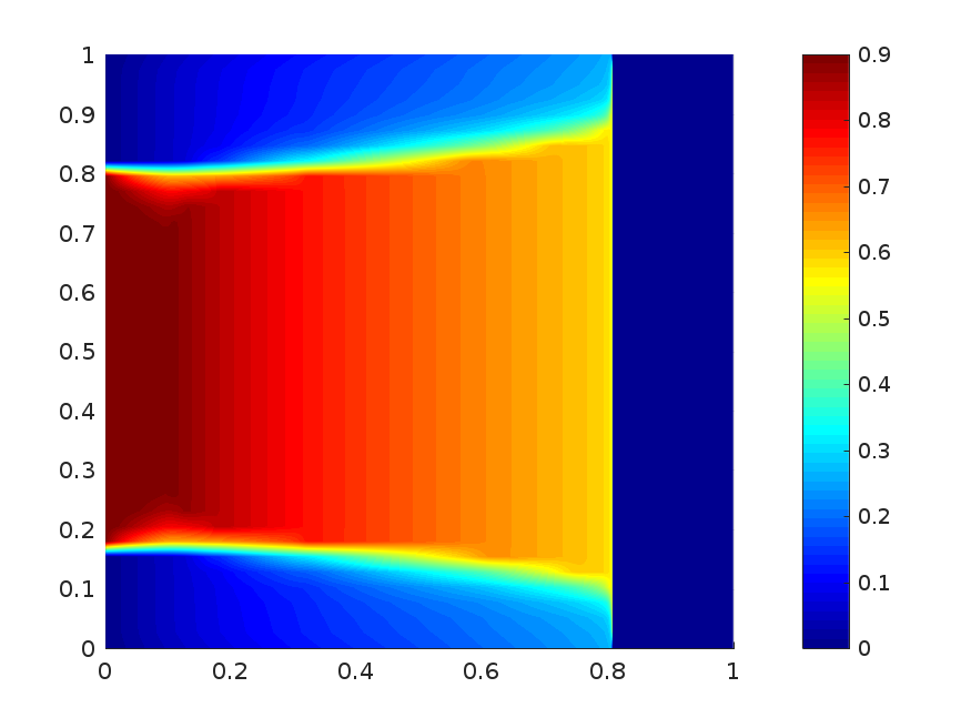
Refer to caption
(a) VE-model
Refer to caption
(b) BVE-model
Refer to caption
(c) Middle Layer
Figure 11: Numerical solution of the VE-model in (a), the BVE-model in (b) and saturation profile in the middle layer for both models in (c), using M=2,βx=βz=106,Nx=2000formulae-sequenceformulae-sequence𝑀2subscript𝛽𝑥subscript𝛽𝑧superscript106subscript𝑁𝑥2000M=2,\,\beta_{x}=\beta_{z}=10^{-6},\,N_{x}=2000, Nz=40subscript𝑁𝑧40N_{z}=40, and T=0.6𝑇0.6T=0.6.

6 Summary

We studied two-phase flow for Darcy and Brinkman regimes. In Darcy regimes, we presented different models that utilize the extreme geometry of asymptotically flat domains to reduce the computational complexity of the two-phase flow model: the VI-model, the VE-model and the Multiscale model. We performed several numerical comparisons of the models and found out that the VE-model shows excellent agreement with the full two-phase flow model, while still being computationally more efficient. On the contrary, the VI-model shows limited accuracy. In addition to the numerical comparisons, we proved the equivalence between the VE-model and the Multiscale model.

In flat domains of Brinkman type, we applied asymptotic analysis to the dimensionless BTP-model. We derived the BVE-model, which is a nonlocal evolution equation for saturation only. It involves a third-order term of mixed-time and spatial- derivatives. We showed by numerical examples that the BVE-model is a proper reduction of the full BTP-model in flat domains. The BVE-model has a similar structure as the model in HG1993 , for which dynamical capillarity effects drive overshooting. Here overshooting occurs within a completely different physical regime.

Acknowledgements.
The first author would like to thank the DAAD for the financial support.

References

  • [1] A. Armiti-Juber and C. Rohde. Almost parallel flows in porous media, Finite Volumes for Complex Applications VII-Elliptic, Parabolic and Hyperbolic Problems, pages 873–881. Springer International Publishing, 2014.
  • [2] J. L. Auriault. On the domain of validity of Brinkman’s equation. Transport Porous Med., 79(2):215–223, 2009.
  • [3] J. L. Auriault, C. Geindreau, and C. Boutin. Filtration law in porous media with poor separation of scales. Transport Porous Med., 60(1):89–108, 2005.
  • [4] J. Bear. Dynamics of fluids in porous media. Dover, 1988.
  • [5] B. Becker, B. Guo, K. Bandilla, M. A. Celia, B. Flemisch, and R. Helmig. A pseudo vertical equilibrium model for slow gravity drainage dynamics. Water Resour. Res., 2017.
  • [6] H. C. Brinkman. A calculation of the viscous force exerted by a flowing fluid on a dense swarm of particles. Appl. Sci. Res., 1(1):27–34, 1949.
  • [7] X. Cao and I. S. Pop. Uniqueness of weak solutions for a pseudo-parabolic equation modeling two phase flow in porous media. Appl. Math. Lett., 46:25–30, 2015.
  • [8] K. H. Coats, J. R. Dempsey, and J. H. Henderson. The use of vertical equilibrium in two-dimensional dimulation of three-dimensional reservoir performance. Soc. Petrol. Eng., 11:63–71, 1971.
  • [9] G. M. Coclite, S. Mishra, N. H. Risebro, and F. Weber. Analysis and numerical approximation of Brinkman regularization of two-phase flows in porous media. Computat. Geosci., 18(5):637–659, 2014.
  • [10] B. Court, K. W. Bandilla, M. A. Celia, A. Janzen, M. Dobossy, and J. M. Nordbotten. Applicability of vertical-equilibrium and sharp-interface assumptions in CO2 sequestration modeling. Int. J. Greenh. Gas Con., 10:134–147, 2012.
  • [11] Y. Debbabi, M. D. Jackson, G. J. Hampson, P. J. R. Fitch, and P. Salinas. Viscous crossflow in layered porous media. Transport Porous Med., 117(2):281–309, Mar 2017.
  • [12] Y. Fan and I. S. Pop. A class of pseudo-parabolic equations: existence, uniqueness of weak solutions, and error estimates for the Euler-implicit discretization. Math. Meth. Appl. Sci., 34(18):2329–2339, 2011.
  • [13] Y. Fan and I.S. Pop. A class of pseudo-parabolic equations: existence, uniqueness of weak solutions, and error estimates for the Euler-implicit discretization. Math. Meth. Appl. Sci., 34(18):2329–2339, 2011.
  • [14] S. E. Gasda, J. M. Nordbotten, and M. A. Celia. Vertical equilibrium with sub-scale analytical methods for geological CO2 sequestration. Computat. Geosci., 13:469–481, 2009.
  • [15] S. E. Gasda, J. M. Nordbotten, and M. A. Celia. Vertically averaged approaches for CO2 migration with solubility trapping. Water Resour. Res., 47, 2011.
  • [16] B. Guo, K. W. Bandilla, F. Doster, E. Keilegavlen, and M. A. Celia. A vertically integrated model with vertical dynamics for CO2 storage. Water Resour. Res., 50(8):6269–6284, 2014.
  • [17] S. M. Hassanizadeh and W. G. Gray. Thermodynamic basis of capillary pressure in porous media. Water Resour. Res., 29:3389–3406, 1993.
  • [18] R. Helmig. Multiphase flow and transport processes in the subsurface. Springer-Verlag, 1997.
  • [19] U. Hornung. Homogenization and porous media. Springer-Verlag, New York, 1997.
  • [20] R. Huber and R. Helmig. Multiphase flow in heterogeneous porous media: A classical finite element method versus an implicit pressure–explicit saturation-based mixed finite element–finite volume approach. Int. J. Numer. Meth. Fluids, 29(8):899–920, 1999.
  • [21] F. Kissling and C. Rohde. The computation of nonclassical shock waves in porous media with a heterogeneous multiscale method: The multidimensional case. Multiscale Model. Simul., 13 no. 4:1507–1541, 2015.
  • [22] L. W. Lake. Enhanced oil recovery. Prentice Hall Englewood Cliffs, N.J, 1989.
  • [23] G. Menon and F. Otto. Dynamic scaling in miscible viscous fingering. Communications in Mathematical Physics, 257(2):303–317, 2005.
  • [24] C. Z. Qin and S. M. Hassanizadeh. Multiphase flow through multilayers of thin porous media: General balance equations and constitutive relationships for a solid–gas–liquid three-phase system. Int. J. Heat Mass Transf., 70:693–708, 2014.
  • [25] C. J. van Duijn, Y. Fan, L. A. Peletier, and I. S. Pop. Travelling wave solutions for degenerate pseudo-parabolic equations modelling two-phase flow in porous media. Nonlinear Anal. Real World Appl., 14(3):1361–1383, 2013.
  • [26] M. T. van Genuchten. A closed-form equation for predicting the hydraulic conductivity of unsaturated soils. Soil sci. soc. Am. j., 44(5):892–898, 1980.
  • [27] Z. Yang and Y. C. Yortsos. Asymptotic solutions of miscible displacements in geometries of large aspect ratio. Phys. Fluids, 9(2):286–298, 1997.
  • [28] Y. Yokoyama and L. W. Lake. The effects of capillary pressure on immiscible displacements in stratified porous media. Soc. Petrol. Eng., 1981.
  • [29] Y. C. Yortsos. A theoretical analysis of vertical flow equilibrium. Transport Porous Med., 18:107–129, 1995.
  • [30] Y. C. Yortsos and D. Salin. On the selection principle for viscous fingering in porous media. J. Fluid Mech., 557:225–236, 2006.
  • [31] V. J. Zapata and L. W. Lake. A theoretical analysis of viscous crossflow. Soc. Petrol. Eng., 1981.
  • [32] X. Zhang, A. Shapiro, and E. H. Stenby. Upscaling of two-phase immiscible flows in communicating stratified reservoirs. Transport Porous Med., 87(3):739–764, Apr 2011.
  • [33] X. Zhang, A. Shapiro, and E. H. Stenby. Gravity effect on two-phase immiscible flows in communicating layered reservoirs. Transport Porous Med., 92(3):767–788, Apr 2012.