Energy flow polynomials:
A complete linear basis for jet substructure

Abstract

We introduce the energy flow polynomials: a complete set of jet substructure observables which form a discrete linear basis for all infrared- and collinear-safe observables. Energy flow polynomials are multiparticle energy correlators with specific angular structures that are a direct consequence of infrared and collinear safety. We establish a powerful graph-theoretic representation of the energy flow polynomials which allows us to design efficient algorithms for their computation. Many common jet observables are exact linear combinations of energy flow polynomials, and we demonstrate the linear spanning nature of the energy flow basis by performing regression for several common jet observables. Using linear classification with energy flow polynomials, we achieve excellent performance on three representative jet tagging problems: quark/gluon discrimination, boosted $W$ tagging, and boosted top tagging. The energy flow basis provides a systematic framework for complete investigations of jet substructure using linear methods.

1 Introduction

Jet substructure is the analysis of radiation patterns and particle distributions within the collimated sprays of particles (jets) emerging from high-energy collisions Seymour:1991cb ; Seymour:1993mx ; Butterworth:2002tt ; Butterworth:2007ke ; Butterworth:2008iy . Jet substructure is central to many analyses at the Large Hadron Collider (LHC), finding applications in both Standard Model measurements Chatrchyan:2012sn ; CMS:2013cda ; Aad:2015lxa ; Aad:2015cua ; TheATLAScollaboration:2015ynv ; Aad:2015hna ; Aad:2015rpa ; ATLAS:2016dpc ; ATLAS:2016wlr ; ATLAS:2016wzt ; CMS:2016rtp ; Rauco:2017xzb ; ATLAS:2017jiz ; Sirunyan:2017dgc and in searches for physics beyond the Standard Model CMS:2011bqa ; Chatrchyan:2012ku ; Fleischmann:2013woa ; Pilot:2013bla ; TheATLAScollaboration:2013qia ; CMS:2014afa ; CMS:2014aka ; Khachatryan:2015axa ; TheATLAScollaboration:2015elo ; TheATLAScollaboration:2015xqi ; Khachatryan:2015bma ; CMS:2016qwm ; CMS:2016bja ; CMS:2016ehh ; CMS:2016rfr ; Aaboud:2016okv ; Khachatryan:2016mdm ; CMS:2016flr ; CMS:2016pod ; Aaboud:2016qgg ; Sirunyan:2016wqt ; Sirunyan:2017usq ; Sirunyan:2017acf ; Sirunyan:2017nvi . An enormous catalog of jet substructure observables has been developed to tackle specific collider physics tasks Abdesselam:2010pt ; Altheimer:2012mn ; Altheimer:2013yza ; Adams:2015hiv ; Larkoski:2017jix , such as the identification of boosted heavy particles or the discrimination of quark- from gluon-initiated jets.

The space of possible jet substructure observables is formidable, with few known complete and systematic organizations. Previous efforts to define classes of observables around organizing principles include: the jet energy moments and related Zernike polynomials to classify energy flow observables GurAri:2011vx ; a pixelated jet image Cogan:2014oua to represent energy deposits in a calorimeter; the energy correlation functions (ECFs) Larkoski:2013eya to highlight the $N$-prong substructure of jets; the generalized energy correlation functions (ECFGs) Moult:2016cvt based around soft-collinear power counting Larkoski:2014gra ; and a set of $N$-subjettiness observables Thaler:2010tr ; Thaler:2011gf ; Stewart:2010tn to capture $N$-body phase space information Datta:2017rhs . With any of these representations, there is no simple method to combine individual observables, so one typically uses sophisticated multivariate techniques such as neural networks to fully access the information contained in several observables Gallicchio:2010dq ; Gallicchio:2011xq ; Gallicchio:2012ez ; Baldi:2014kfa ; Baldi:2014pta ; deOliveira:2015xxd ; Barnard:2016qma ; Komiske:2016rsd ; Kasieczka:2017nvn ; Almeida:2015jua ; Baldi:2016fql ; Guest:2016iqz ; Louppe:2017ipp ; Pearkes:2017hku ; Butter:2017cot ; Aguilar-Saavedra:2017rzt ; Datta:2017rhs . Furthermore, the sense in which these sets “span” the space of jet substructure is often unclear, sometimes relying on the existence of complicated nonlinear functions to map observables to kinematic phase space.

In this paper, we introduce a powerful set of jet substructure observables organized directly around the principle of infrared and collinear (IRC) safety. These observables are multiparticle energy correlators with specific angular structures which directly result from IRC safety. Since they trace their lineage to the hadronic energy flow analysis of Ref. Tkachov:1995kk , we call these observables the energy flow polynomials (EFPs) and we refer to the set of EFPs as the energy flow basis. In the language of Ref. Tkachov:1995kk , the EFPs can be viewed as a discrete set of $C$-correlators, though our analysis is independent from the original $C$-correlator logic. Crucially, the EFPs form a linear basis of all IRC-safe observables, making them suitable for a wide variety of jet substructure contexts where linear methods are applicable.

There is a one-to-one correspondence between EFPs and loopless multigraphs, which helps to visualize and calculate the EFPs. A multigraph is a graph where any two vertices can be connected by multiple edges; in this context, a loop is an edge from a vertex to itself, while a closed chain of edges is instead referred to as a cycle. For a multigraph $G$ with $N$ vertices and edges $(k,\ell)\in G$, the corresponding EFP takes the form:

$$\text{EFP}_{G}=\sum_{i_{1}=1}^{M}\cdots\sum_{i_{N}=1}^{M}z_{i_{1}}\cdots z_{i_{N}}\prod_{(k,\ell)\in G}\theta_{i_{k}i_{\ell}},$$ (1)

where the jet consists of $M$ particles, $z_{i}\equiv E_{i}/\sum_{j=1}^{M}E_{j}$ is the energy fraction carried by particle $i$, and $\theta_{ij}$ is the angular distance between particles $i$ and $j$. The precise definitions of $E_{i}$ and $\theta_{ij}$ will depend on the collider context, with energy and spherical ($\theta,\phi$) coordinates typically used for $e^{+}e^{-}$ collisions, and transverse momentum $p_{T}$ and rapidity-azimuth $(y,\phi)$ coordinates for hadronic collisions. For brevity, we often use the multigraph $G$ to represent the formula for $\text{EFP}_{G}$ in Eq. (1), e.g.:

$$\begin{gathered}\includegraphics[scale={.3}]{graphs/5_7_9}\end{gathered}=\sum_{i_{1}=1}^{M}\sum_{i_{2}=1}^{M}\sum_{i_{3}=1}^{M}\sum_{i_{4}=1}^{M}\sum_{i_{5}=1}^{M}z_{i_{1}}z_{i_{2}}z_{i_{3}}z_{i_{4}}z_{i_{5}}\theta_{i_{1}i_{2}}\theta_{i_{2}i_{3}}\theta_{i_{1}i_{3}}\theta_{i_{1}i_{4}}\theta_{i_{1}i_{5}}\theta_{i_{4}i_{5}}^{2}.$$ (2)

This paper is a self-contained introduction to the energy flow basis, with the following organization. Sec. 2 contains a general overview of the EFPs, with more detailed descriptions of Eq. (1) and the correspondence to multigraphs. We also discuss a few different choices of measure for $z_{i}$ and $\theta_{ij}$. As already mentioned, EFPs are a special case of $C$-correlators Tkachov:1995kk , so not surprisingly, we find a close relationship between EFPs and other classes of observables that are themselves $C$-correlators, including jet mass, ECFs Larkoski:2013eya , certain generalized angularities Larkoski:2014pca , and energy distribution moments GurAri:2011vx . We also highlight features of the EFPs which are less well-known in the $C$-correlator-based literature.

In Sec. 3, we give a detailed derivation of the EFPs as an (over)complete linear basis of all IRC-safe observables in the case of massless particles. Because this section is rather technical, it can be omitted on a first reading, though the logic just amounts to systematically imposing the constraints of IRC safety. In Sec. 3.1, we use an independent (and arguably more transparent) logic from Ref. Tkachov:1995kk to show that any IRC-safe observable can be written as a linear combination of $C$-correlators:

$$\mathcal{C}_{N}^{f_{N}}=\sum_{i_{1}=1}^{M}\cdots\sum_{i_{N}=1}^{M}E_{i_{1}}\cdots E_{i_{N}}\,f_{N}(\hat{p}_{i_{1}}^{\mu},\ldots,\hat{p}_{i_{N}}^{\mu}),$$ (3)

where $f_{N}$ is an angular weighting function that is only a function of the particle directions $\hat{p}_{i}^{\mu}=p_{i}^{\mu}/E_{i}$ (and not their energies $E_{i}$). To derive Eq. (3), we use the Stone-Weierstrass theorem stone1948generalized to expand an arbitrary IRC-safe observable in polynomials of particle energies, and then directly impose IRC safety and particle relabeling invariance. In Sec. 3.2, we determine the angular structures of the EFPs by expanding $f_{N}$ in terms of a discrete set of polynomials in pairwise angular distances. Remarkably, the discrete set of polynomials appearing in this expansion is in one-to-one correspondence with the set of non-isomorphic multigraphs, which facilitates indexing the EFPs by multigraphs to encode the geometric structure in Eq. (1).

In Sec. 4, we investigate the complexity of computing EFPs. Naively, Eq. (1) has complexity $\mathcal{O}(M^{N})$ due to the $N$ nested sums over $M$ particles. However, the rich analytic structure of Eq. (1) and the graph representations of EFPs allow for numerous algorithmic speedups. Any EFP with a disconnected graph can be computed as the product of the EFPs corresponding to its connected components. Furthermore, we find that the Variable Elimination (VE) algorithm zhang1996exploiting can be used to vastly speed up the computation of many EFPs compared to the naive $\mathcal{O}(M^{N})$ algorithm. VE uses the factorability of the summand to systematically determine a more efficient order for performing nested sums. For instance, all tree graphs can be computed in $\mathcal{O}(M^{2})$ using VE. As an explicit example, consider an EFP with naive $\mathcal{O}(M^{6})$ scaling:

$$\begin{gathered}\includegraphics[scale={.25}]{graphs/6_5_2}\end{gathered}\,=\sum_{i_{1}=1}^{M}\sum_{i_{2}=1}^{M}z_{i_{1}}z_{i_{2}}\theta_{i_{1}i_{2}}\left(\sum_{i_{3}=1}^{M}z_{i_{3}}\theta_{i_{1}i_{3}}\right)^{2}\left(\sum_{i_{4}=1}^{M}z_{i_{4}}\theta_{i_{2}i_{4}}\right)^{2}.$$ (4)

The quantities in parentheses are computable in $\mathcal{O}(M^{2})$, since they are length $M$ lists with each element a sum over $M$ objects, making the overall expression in Eq. (4) computable in $\mathcal{O}(M^{2})$. The efficient computation of the EFPs overcomes one of the main previous challenges in using higher-$N$ multiparticle correlators in collider physics applications.

In Sec. 5, we perform numerical linear regression with EFPs for various jet observables. The linear spanning nature of the energy flow basis means that any IRC-safe observable $\mathcal{S}$ can be linearly approximated by EFPs, which we write as:

$$\mathcal{S}\simeq\sum_{G\in\mathcal{G}}s_{G}\,\text{EFP}_{G},$$ (5)

for some finite set of multigraphs $\mathcal{G}$ and some real coefficients $s_{G}$. One might worry that the number of EFPs needed to achieve convergence could be intractably large. In practice, though, we find that the required set of $\mathcal{G}$ needed for convergence is rather reasonable in a variety of jet contexts. While we find excellent convergence for IRC-safe observables, regressing with IRC-unsafe observables does not work as well, demonstrating the importance of IRC safety for the energy flow basis.

In Sec. 6, we perform another test of Eq. (5) by using linear classification with EFPs to distinguish signal from background jets. We consider three representative jet tagging problems: quark/gluon discrimination, boosted $W$ tagging, and boosted top tagging. In this study, the observable appearing on the left-hand side of Eq. (5) is the optimal IRC-safe discriminant for the two classes of jets. Remarkably, linear classification with EFPs performs comparably to multivariate machine learning techniques, such as jet images with convolutional neural networks (CNNs) Cogan:2014oua ; deOliveira:2015xxd ; Barnard:2016qma ; Komiske:2016rsd ; Kasieczka:2017nvn or dense neural networks (DNNs) with a complete set of $N$-subjettiness observables Datta:2017rhs . Both the linear regression and classification models have few or no hyperparameters, illustrating the power and simplicity of linear learning methods combined with our fully general linear basis for IRC-safe jet substructure.

Our conclusions are presented in Sec. 7, where we highlight the relevance of the energy flow basis to machine learning and discuss potential future applications and developments. A review of $C$-correlators and additional tagging plots are left to the appendices.

2 Energy flow polynomials

IRC-safe observables have long been of theoretical and experimental interest because observables which lack IRC safety are not well defined Kinoshita:1962ur ; Lee:1964is ; Weinberg:1995mt ; sterman1995handbook , or require additional care to calculate Larkoski:2013paa ; Larkoski:2015lea ; Waalewijn:2012sv ; Chang:2013rca ; Elder:2017bkd , in perturbative quantum chromodynamics (pQCD). More broadly, though, IRC safety is a simple and natural organizing principle for high-energy physics observables, since IRC-safe observables probe the high-energy structure of an event while being insensitive to low-energy and collinear modifications. IRC safety is also an important property experimentally as IRC-safe observables are more robust to noise and finite detector granularity.

As argued in Refs. Tkachov:1995kk ; Sveshnikov:1995vi ; Cherzor:1997ak ; Tkachov:1999py , the $C$-correlators in Eq. (3) are a generic way to capture the IRC-safe structure of a jet, as long as one chooses an appropriate angular weighting function $f_{N}$. Later in Sec. 3, we give an alternative proof that $C$-correlators span the space of IRC-safe observables and go on to give a systematic expansion for $f_{N}$. This expansion results in the EFPs, which yield an (over)complete linear basis for IRC-safe observables. In this section, we highlight the basic features of the EFPs and their relationship to previous jet substructure observables.

2.1 The energy flow basis

One can think of the EFPs as $C$-correlators that make specific, discrete choices for the angular weighting function $f_{N}$ in Eq. (3). True to their name, EFPs have angular weighting functions that are polynomial in pairwise angular distances $\theta_{ij}$. The energy flow basis is therefore all $C$-correlators with angular structures that are unique monomials in $\theta_{ij}$, meaning monomials that give algebraically different expressions once the sums in Eq. (3) are performed. Since we intend to apply the energy flow basis for jet substructure, we remove the dependence on the overall jet kinematics by normalizing the particle energies by the total jet energy, $E_{J}\equiv\sum_{i=1}^{M}E_{i}$, leading to the EFPs written in terms of the energy fractions $z_{i}\equiv E_{i}/E_{J}$ as in Eq. (1).

The uniqueness requirement on angular monomials can be better understood by developing a correspondence between monomials in $\theta_{ij}$ and multigraphs:

Multigraph/EFP Correspondence.

The set of loopless multigraphs on $N$ vertices corresponds exactly to the set of angular monomials in $\{\theta_{i_{k}i_{\ell}}\}_{k<\ell\in\{1,\cdots,N\}}$. Each edge $(k,\ell)$ in a multigraph is in one-to-one correspondence with a term $\theta_{i_{k}i_{\ell}}$ in an angular monomial; each vertex $j$ in the multigraph corresponds to a factor of $z_{i_{j}}$ and summation over $i_{j}$ in the EFP:

$$\begin{gathered}\includegraphics[scale={0.04}]{graphs/dot}\end{gathered}_{j}\,\,\Longleftrightarrow\,\,\sum_{i_{j}=1}^{M}z_{i_{j}}, k\begin{gathered}\includegraphics[scale={0.3}]{graphs/line}\end{gathered}\,\ell\,\,\Longleftrightarrow\,\,\theta_{i_{k}i_{\ell}}.$$ (8)

Using Eq. (8), the EFPs can be directly encoded by their corresponding multigraphs. For instance:

$$\begin{gathered}\includegraphics[scale={0.32}]{graphs/4_5_9}\end{gathered}=\sum_{i_{1}=1}^{M}\sum_{i_{2}=1}^{M}\sum_{i_{3}=1}^{M}\sum_{i_{4}=1}^{M}z_{i_{1}}z_{i_{2}}z_{i_{3}}z_{i_{4}}\theta_{i_{1}i_{2}}\theta_{i_{2}i_{3}}\theta_{i_{2}i_{4}}^{2}\theta_{i_{3}i_{4}}.$$ (9)

Since any labeling of the vertices gives an equivalent algebraic expression, we represent the graphs as unlabeled. The specification that the EFPs are unique monomials translates into the requirement that the corresponding multigraphs are non-isomorphic. Versions of these multigraphs have previously appeared in the physics literature in the context of many-body configurations dallot1992reduced ; mandal2017determination , encoding all local scalar operators of a free theory Hogervorst:2014rta , and in graphically depicting ECFs for jets Moult:2016cvt ; Larkoski:2017iuy .

	Multigraph		Energy Flow Polynomial
$N$ :	Number of vertices	$\Longleftrightarrow$	$N$-particle correlator
$d$ :	Number of edges	$\Longleftrightarrow$	Degree of angular monomial
$\chi$ :	Treewidth $+\,1$	$\Longleftrightarrow$	Optimal VE complexity $\mathcal{O}(M^{\chi})$
	Chromatic number	$\Longleftrightarrow$	Minimum number of prongs to not vanish
	Connected	$\Longleftrightarrow$	Prime
	Disconnected	$\Longleftrightarrow$	Composite

Table 1: Corresponding properties of multigraphs and EFPs.

Table 1 contains a summary of the correspondence between the properties of EFPs and multigraphs. The number of graph vertices $N$ corresponds to the number of particle sums in the EFP, and the number of graph edges $d$ corresponds to the degree of the EFP (i.e. the degree of the underlying angular monomial). The number of separated prongs for which an individual EFP is first non-vanishing is the chromatic number of the graph: the smallest number of colors needed to color the vertices of the graph with no two adjacent vertices sharing a color. For computational reasons discussed further in Sec. 4, we also care about the treewidth of the graph, which is related to the computational complexity $\chi$ of an EFP. Also for computational reasons, we make a distinction between connected or prime multigraphs and disconnected or composite multigraphs; the value of a composite EFP is simply the product of the prime EFPs corresponding to its connected components.

Maximum degree $d$		0	1	2	3	4	5	6	7	8	9	10
Prime EFPs	A076864	1	1	2	5	12	33	103	333	1 183	4 442	17 576
	Cumul.	1	2	4	9	21	54	157	490	1 673	6 115	23 691
All EFPs	A050535	1	1	3	8	23	66	212	686	2 389	8 682	33 160
	Cumul.	1	2	5	13	36	102	314	1 000	3 389	12 071	45 231

(a)

$d$		1	2	3	4	5	6	7	8	9	10
$N$	2	1	1	1	1	1	1	1	1	1	1
	3		1	2	3	4	6	7	9	11	13
	4			2	5	11	22	37	61	95	141
	5				3	11	34	85	193	396	771
	6					6	29	110	348	969	2 445
	7						11	70	339	1 318	4 457
	8							23	185	1 067	4 940
	9								47	479	3 294
	10									106	1 279
	11										235

(b)

Table 2: (a) The number of EFPs (prime and all) organized by degree $d$, for $d$ up to 10. The cumulative rows tally the number of EFPs with degree at most $d$, i.e. the number of basis elements truncated at that $d$. While these sequences grow quickly, the total number of all basis elements is at most 1000 for $d\leq 7$, which is computationally tractable. (b) The number of prime EFPs broken down by number of vertices $N$ and number of edges $d$ in the multigraph. All connected graphs (prime EFPs) for $d$ up to 5 are shown explicitly in Table 3.

Because the EFP basis is infinite, a suitable organization and truncation scheme is necessary to use the basis in practice. In this paper, we usually truncate by restricting to the set of all multigraphs with at most $d$ edges. This is a natural choice because it corresponds to truncating the approximation of the angular function $f_{N}$ at degree $d$ polynomials. Furthermore, this truncation results in a finite number of EFPs at each order of truncation, which is not true for truncation by the number of vertices. The number of multigraphs with exactly $d$ edges is Sequence A050535 in the On-Line Encyclopedia of Integer Sequences (OEIS) sloane2007line ; harary2014graphical ; the number of connected multigraphs with exactly $d$ edges is Sequence A076864 in the OEIS sloane2007line . The numbers of EFPs in our truncation of the energy flow basis are the partial sums of these sequences, which are listed in Table 2a up to $d=10$. Table 2b tabulates the number of prime EFPs of degree $d$ binned by $N$ up to $d=10$. Table 3 illustrates all connected multigraphs with $d\leq 5$ edges.

Degree	Connected Multigraphs
$d=0$
$d=1$
$d=2$
$d=3$
$d=4$
$d=5$

Table 3: All non-isomorphic, loopless, connected multigraphs organized by the total number of edges $d$, up to $d=5$, sorted by their number of vertices $N$. Note that for a fixed number of edges $d$, the total number of multigraphs (connected or not) is finite. These graphs correspond to the $d\leq 5$ prime EFPs counted in Table 2a. Image files for all of the prime EFP multigraphs up to $d=7$ are available here.

2.2 Energy and angular measures

There are many possible choices for the energy fraction $z_{i}$ and angular measure $\theta_{ij}$ used to define the EFPs. In the analysis of Sec. 3, this choice arises because there are many systematic expansions of IRC-safe observables in terms of energy-like and angular-like quantities. Typically, one wants to work with observables that respect the appropriate Lorentz subgroup for the collision type of interest. For $e^{+}e^{-}$ colliders, the symmetries are the group of rotations about the interaction point, and for hadron colliders they are rotations about and boosts along the beam axis (sometimes with a reflection in the plane perpendicular to the beam). Therefore, the energy fractions $z_{i}$ usually use particle energies $E_{i}$ at an $e^{+}e^{-}$ collider and particle transverse momenta $p_{T,i}$ at a hadron collider.

For the angular weighting function $f_{N}$, though, there are many different angular structures one can build out of the particle directions $\hat{p}^{\mu}_{i}$. The EFPs use the simplest and arguably most natural choice to expand the angular behavior: pairwise angular distances $\theta_{ij}$, determined using spherical coordinates $(\theta,\phi)$ at an $e^{+}e^{-}$ collider and rapidity-azimuth coordinates $(y,\phi)$ at a hadron collider. Other classes of observables, such as ECFs Larkoski:2013eya and ECFGs Moult:2016cvt , also use pairwise angles since they manifestly respect the underlying Lorentz subgroup. For building the EFPs, is important that the $\theta_{ij}$, or any other choice of geometric object, be sufficient to reconstruct the value of the original function $f_{N}$ in terms of the $\hat{p}_{i}^{\mu}$. For pairwise angles, this property can be shown by triangulation, under the assumption that the observable in question does not depend on the overall jet direction nor on rotations or reflections about the jet axis. Since jets are collimated sprays of particles, the $\theta_{ij}$ are typically small and are good expansion parameters.

At various points in this paper, we explore three different energy/angular measures. For $e^{+}e^{-}$ collisions, our default is:

$$\boxed{\text{$e^{+}e^{-}$ Default}}\qquad\begin{aligned} \quad z_{i}&=\frac{E_{i}}{E_{J}},\qquad E_{J}\equiv\sum_{i=1}^{M}E_{i},\\ \theta_{ij}&=\left(\frac{2\,p_{i}^{\mu}p_{j\mu}}{E_{i}E_{j}}\right)^{\beta/2},\end{aligned}$$ (10)

where $\beta>0$ is an angular weighting factor. For the hadron collider studies in Secs. 5 and 6, we use:

$$\boxed{\text{Hadronic Default}}\qquad\begin{aligned} \quad z_{i}&=\frac{p_{T,i}}{p_{T,J}},\qquad p_{T,J}\equiv\sum_{i=1}^{M}p_{T,i},\\ \theta_{ij}&=\left(\Delta y_{ij}^{2}+\Delta\phi_{ij}^{2}\right)^{\beta/2},\end{aligned}$$ (11)

where $\Delta y_{ij}\equiv y_{i}-y_{j}$, $\Delta\phi_{ij}\equiv\phi_{i}-\phi_{j}$ are determined by the rapidity $y_{i}$ and azimuth $\phi_{i}$ of particle $i$. This measure is rotationally-symmetric in the $(y,\phi)$ plane, which is the most commonly used case in jet substructure. For situations where this rotational symmetry is not desirable (such as for jet pull Gallicchio:2010sw ), we can instead use a two-dimensional measure that treats the rapidity and azimuthal directions separately:

$$\boxed{\text{Hadronic Two-Dimensional}}\qquad\begin{aligned} \quad z_{i}&=\frac{p_{T,i}}{p_{T,J}},\qquad p_{T,J}\equiv\sum_{i=1}^{M}p_{T,i},\\ \theta_{ij}&=\Delta y_{ij}\text{ or }\Delta\phi_{ij},\end{aligned}$$ (12)

where each line on the multigraph now has an additional decoration to indicate whether it corresponds to $\Delta y$ or $\Delta\phi$.

We emphasize that the choice of measure is not unique, though it is constrained by the IRC-safety arguments in Sec. 3. For example, IRC safety requires that the energy-like quantities appear linearly in $z_{i}$. For the default measures, the angular exponent $\beta$ can take on any positive value and still be consistent with IRC safety. Depending on the context, different choices of $\beta$ can lead to faster or slower convergence of the EFP expansion, with $\beta<1$ emphasizing smaller values of $\theta_{ij}$ and $\beta>1$ emphasizing larger values of $\theta_{ij}$. For special choices of $z_{i}$ and $\theta_{ij}$, some EFPs may be linearly related, a point we return to briefly in Sec. 4.1.

2.3 Relation to existing substructure observables

Many familiar jet observables can be nicely interpreted in the energy flow basis. When an observable can be written as a simple expression in terms of particle four-momenta or in terms of energies and angles, the energy flow decomposition can often be performed exactly. Some of the most well-known observables, such as jet mass and energy correlation functions, are exactly finite linear combinations of EFPs (with appropriate choice of measure), which one might expect since they also correspond to natural $C$-correlators. Unless otherwise specified, the analysis below uses the default hadronic measure in Eq. (11) with $\beta=1$ and treats all particles as massless.

2.3.1 Jet mass

Jet mass is most basic jet substructure observable, and not surprisingly, it has a nice expansion in the energy flow basis. In particular, the squared jet mass divided by the jet energy squared is an exact $N=2$ EFP using the $e^{+}e^{-}$ measure in Eq. (10) with $\beta=1$:

$$e^{+}e^{-}:\qquad\frac{m_{J}^{2}}{E_{J}^{2}}=\frac{1}{2}\sum_{i_{1}=1}^{M}\sum_{i_{2}=1}^{M}z_{i_{1}}z_{i_{2}}\left(\frac{2\,p_{i_{1}}^{\mu}p_{i_{2}\mu}}{E_{i_{1}}E_{i_{2}}}\right)=\frac{1}{2}\times\begin{gathered}\includegraphics[scale={.2}]{graphs/2_2_1}\end{gathered}.$$ (13)

Note that mass is exactly an EFP for any $\beta=2/N$ measure choice.

For the hadronic measure in Eq. (11) with $\beta=1$, there is an approximate equivalence with the squared jet mass divided by the jet (scalar) transverse momentum:

$$\text{Hadronic}:\qquad\frac{m_{J}^{2}}{p_{TJ}^{2}}=\sum_{i_{1}=1}^{M}\sum_{i_{2}=1}^{M}z_{i_{1}}z_{i_{2}}(\cosh(\Delta y_{i_{1}i_{2}})-\cos(\Delta\phi_{i_{1}i_{2}}))=\frac{1}{2}\times\begin{gathered}\includegraphics[scale={.2}]{graphs/2_2_1}\end{gathered}+\cdots.$$ (14)

Since the jet mass is not exactly rotationally symmetric in the rapidity-azimuth plane, the subleading terms in Eq. (14) are not fully encompassed by the simplified set of hadronic observables depending only on $\{\Delta y_{ij}^{2}+\Delta\phi_{ij}^{2}\}$, but could be fully encompassed by using an expansion in $\{\Delta y_{ij},\Delta\phi_{ij}\}$ as in Eq. (12). For narrow jets, these higher-order terms in the expansion become less relevant since $\Delta y_{ij},\,\Delta\phi_{ij}\ll 1$.

2.3.2 Energy correlation functions

The ECFs are designed to be sensitive to $N$-prong jet substructure Larkoski:2013eya . They can be written as a $C$-correlator, Eq. (3), with a particular choice of angular weighting function:

$$f_{N}^{(\beta)}(\{\theta_{ij}\})=\prod_{i<j}\theta^{\beta}_{ij},$$ (15)

where $\theta_{ij}=(\Delta y_{ij}^{2}+\Delta\phi_{ij}^{2})^{1/2}$. In terms of multigraphs, the ECFs correspond to complete graphs on $N$ vertices:

$$e_{2}^{(\beta)}=\begin{gathered}\includegraphics[scale={.2}]{graphs/2_1_1}\end{gathered}\,,\hskip 36.135pte_{3}^{(\beta)}=\begin{gathered}\includegraphics[scale={.2}]{graphs/3_3_1}\end{gathered}\,,\hskip 36.135pte_{4}^{(\beta)}=\begin{gathered}\includegraphics[scale={.2}]{graphs/4_6_1}\end{gathered},$$ (16)

which are EFPs using the measure in Eq. (11) with exponent $\beta$.

The ECFs have since been expanded to a more flexible set of observables referred to as the ECFGs Moult:2016cvt . Letting $\min^{(m)}$ indicate the $m$-th smallest element in a set, the ECFGs are also $C$-correlators with angular weighting function:

$$\,_{v}f_{N}^{(\beta)}(\{\theta_{ij}\})=\prod_{m=1}^{v}\min_{i<j}^{(m)}\{\theta^{\beta}_{ij}\}.$$ (17)

The ECFGs do not have an exact multigraph correspondence due to the presence of the min function, but are evidently closely related to the EFPs since they share a common energy structure. The min function itself can be approximated by polynomials in its arguments, which induces an approximating series for the ECFGs in terms of EFPs when plugged into the common energy structure.

Both the EFPs and the ECFGs represent natural extensions of the ECFs but in different directions. From our graph-theoretic perspective, the EFPs extend the ECFs to non-fully-connected graphs. The ECFGs extend the scaling properties of the ECFs into observables with independent energy and angular scalings. As discussed in Sec. 2.4, there are angular structures possible in the EFPs that are not possible in the ECFGs. As with any jet substructure analysis, the choice of which set of observables to use depends on the physics of interest, with the EFPs designed for linear completeness and the ECFGs designed for nice power-counting properties.

2.3.3 Angularities

Next, we consider the IRC-safe jet angularities Larkoski:2014pca (see also Refs. Berger:2003iw ; Almeida:2008yp ; Ellis:2010rwa ; Larkoski:2014uqa ) defined by:

$$\lambda^{(\alpha)}=\sum_{i=1}^{M}z_{i}\,\theta_{i}^{\alpha},$$ (18)

where $\alpha>0$ is an angular exponent and $\theta_{i}$ denotes the distance of particle $i$ to the jet axis. For concreteness and analytic tractability, we take the jet axis to be the $p_{T}$-weighted centroid in $(y,\phi)$-space, such that the jet axis is located at:

$$y_{J}=\sum_{j=1}^{M}z_{j}y_{j},\qquad\phi_{J}=\sum_{j=1}^{M}z_{j}\phi_{j}.$$ (19)

With this, the angularities can be expressed as:

$$\lambda^{(\alpha)} =\sum_{i_{1}=1}^{M}z_{i_{1}}\left((y_{i_{1}}-y_{J})^{2}+(\phi_{i_{1}}-\phi_{J})^{2}\right)^{\alpha/2}$$

$$=\sum_{i_{1}=1}^{M}z_{i_{1}}\left(\left(\sum_{i_{2}=1}^{M}z_{i_{2}}\Delta y_{i_{1}i_{2}}\right)^{2}+\left(\sum_{i_{2}=1}^{M}z_{i_{2}}\Delta\phi_{i_{1}i_{2}}\right)^{2}\right)^{\alpha/2}$$

$$=\sum_{i_{1}=1}^{M}z_{i_{1}}\left(\sum_{i_{2}=1}^{M}z_{i_{2}}\theta_{i_{1}i_{2}}^{2}-\frac{1}{2}\sum_{i_{2}=1}^{M}\sum_{i_{3}=1}^{M}z_{i_{2}}z_{i_{3}}\theta_{i_{2}i_{3}}^{2}\right)^{\alpha/2}.$$ (20)

For even $\alpha$, the parenthetical in Eq. (20) can be expanded and identified to be a linear combination of EFPs with $N=\alpha$ and $d=\alpha$ (see Ref. GurAri:2011vx for a related discussion). For $\alpha=2$, Eq. (20) implies:

$$\lambda^{(2)}=\frac{1}{2}\sum_{i\in J}\sum_{j\in J}z_{i}z_{j}\theta_{ij}^{2}=\frac{1}{2}\times\begin{gathered}\includegraphics[scale={.2}]{graphs/2_2_1}\end{gathered}.$$ (21)

For $\alpha=4$ and $\alpha=6$, Eq. (20) implies:

$$\lambda^{(4)} =\begin{gathered}\includegraphics[scale={.2}]{graphs/3_4_1}\end{gathered}-\frac{3}{4}\times\begin{gathered}\includegraphics[scale={.2}]{graphs/2_2_1}\includegraphics[scale={.2}]{graphs/2_2_1}\end{gathered},$$ (24)

$$\lambda^{(6)} =\begin{gathered}\includegraphics[scale={.25}]{graphs/4_6_2}\end{gathered}-\frac{3}{2}\times\begin{gathered}\includegraphics[scale={.2}]{graphs/3_4_1}\end{gathered}\begin{gathered}\includegraphics[scale={.2}]{graphs/2_2_1}\end{gathered}\,+\frac{5}{8}\times\begin{gathered}\includegraphics[scale={.2}]{graphs/2_2_1}\includegraphics[scale={.2}]{graphs/2_2_1}\includegraphics[scale={.2}]{graphs/2_2_1}\end{gathered}\,.$$ (29)

This can be continued for arbitrarily high, even $\alpha$. Thus, the even $\alpha$ angularities are exact, non-trivial linear combinations of EFPs, illustrating the close connections between the two classes of observables. While angularities with odd or non-integer $\alpha$ do not have the same analytic tractability, the specific case of $\alpha=1/2$ is shown to be numerically well approximated by EFPs in Sec. 5.3.

2.3.4 Geometric moment tensors

Next, we consider observables based on the two-dimensional geometric moment tensor of the energy distribution in the $(y,\phi)$-plane GurAri:2011vx ; Gallicchio:2012ez :

$${\bf C} =\sum_{i\in J}z_{i}\begin{pmatrix}\Delta y_{i}^{2}&\Delta y_{i}\Delta\phi_{i}\\ \Delta\phi_{i}\Delta y_{i}&\Delta\phi_{i}^{2}\end{pmatrix}=\begin{pmatrix}\frac{1}{2}\sum_{i,j}z_{i}z_{j}\Delta y_{ij}^{2}&\frac{1}{2}\sum_{i,j}z_{i}z_{j}\Delta y_{ij}\Delta\phi_{ij}\\ \frac{1}{2}\sum_{i,j}z_{i}z_{j}\Delta\phi_{ij}\Delta y_{ij}&\frac{1}{2}\sum_{i,j}z_{i}z_{j}\Delta\phi_{ij}^{2}\end{pmatrix},$$ (30)

where the distances are measured with respect to the $p_{T}$-weighted centroid axis $(y_{J},\phi_{J})$ from Eq. (19). Useful observables can be constructed from the trace and determinant of C, such as planar flow $\text{Pf}=4\det{\bf C}/(\operatorname{tr}{\bf C})^{2}$ Thaler:2008ju ; Almeida:2008yp , which is a ratio of two IRC-safe observables.

We see that Eq. (30) is exactly a matrix of EFPs with $N=2$ and the two-dimensional hadronic measure from Eq. (12). The trace $\operatorname{tr}{\bf C}$ and determinant $\det{\bf C}$ have the rotational symmetry in the $(y,\phi)$-plane of the default hadronic measure from Eq. (11), allowing them to be written as linear combinations of EFPs with that measure:

$$\operatorname{tr}\bf C =\frac{1}{2}\times\begin{gathered}\includegraphics[scale={.2}]{graphs/2_2_1}\end{gathered}\,, 4\,\det{\bf C} =\begin{gathered}\includegraphics[scale={.2}]{graphs/3_4_1}\end{gathered}\,-\frac{1}{2}\times\begin{gathered}\includegraphics[scale={.2}]{graphs/2_4_1}\end{gathered}\,.$$ (34)

In Ref. GurAri:2011vx , a general class of energy flow moments was explored and categorized, with the goal of classifying observables according to their energy flow distributions. These energy flow moments are defined with respect to a specified jet axis:

$$I_{k_{1}\cdots k_{N}}\equiv\sum_{i=1}^{M}z_{i}\,x_{k_{1}}^{(i)}\cdots x_{k_{N}}^{(i)},$$ (35)

where $k_{i}\in\{1,2\}$, $x_{1}^{(i)}=\Delta y_{i}=y_{i}-y_{J}$ and $x_{2}^{(i)}=\Delta\phi_{i}=\phi_{i}-\phi_{J}$. Using the $p_{T}$-weighted centroid axis, this is the natural generalization of Eq. (30), with the special case of $I_{k_{1}k_{2}}=({\bf C})_{k_{1}k_{2}}$. By performing a similar analysis to the one used to arrive at Eq. (34), one can show that any scalar constructed by contracting the indices of a product of objects in Eq. (35) can be decomposed into an exact linear combination of EFPs.

2.4 Going beyond existing substructure observables

Because the EFPs are $C$-correlators that span the space of IRC-safe observables, their angular structures should encompass all possible behaviors of $C$-correlators. By contrast, the ECFs and ECFGs mentioned in Sec. 2.3.2 have more restricted behaviors, and it is illuminating to understand the new kinds of structures present in the EFPs.

Without loss of generality, the angular weighting function $f_{N}$ in Eq. (3) can be taken to be a symmetric function of the particle directions $\hat{p}_{i}^{\mu}$ due to the symmetrization provided by the sum structure (see Eq. (52) below). The ECFs and ECFGs exhibit a stronger symmetry, though, since the angular functions in Eqs. (15) and (17) are invariant under the swapping any two pairwise angles $\theta_{ij}$. This symmetry is manifested in the ECFs multigraphs in Eq. (16) by the fact that all pairs of indices are connected by the same number of edges.

We can easily see that the pairwise swap symmetry of the ECFs is stronger than the full permutation symmetry of the EFPs: the group of permutations of the angular distances $\theta_{ij}$ has $\binom{N}{2}!$ elements, whereas the group of permutations of the indices $\{i_{a}\}$ has $N!$ elements. An example of an EFP that does not satisfy the stronger symmetry is the following $N=4$ graph:

$$\begin{gathered}\includegraphics[scale={0.25}]{graphs/4_3_1}\end{gathered}=\sum_{i_{1}=1}^{M}\sum_{i_{2}=1}^{M}\sum_{i_{3}=1}^{M}\sum_{i_{4}=1}^{M}z_{i_{1}}z_{i_{2}}z_{i_{3}}z_{i_{4}}\theta_{i_{1}i_{2}}\theta_{i_{1}i_{3}}\theta_{i_{1}i_{4}}.$$ (36)

The angular weighting function of the EFP in Eq. (36) is symmetric under the $4!$ permutations in the indices (vertices) $i_{a}\to i_{\sigma(a)}$ but not under the exchange of pairwise angles (edges) $\theta_{i_{1}i_{3}}\to\theta_{i_{2}i_{3}}$ which would result in a different EFP, namely:

$$\begin{gathered}\includegraphics[scale={0.2},angle={90}]{graphs/4_3_2}\end{gathered}\neq\begin{gathered}\includegraphics[scale={0.25},angle={0}]{graphs/4_3_1}\end{gathered}.$$ (37)

Another feature of the ECFs and ECFGs is that their angular weighting function $f_{N}$ vanishes whenever two of its arguments become collinear. Indeed, one of the present authors made the erroneous claim in Ref. Moult:2016cvt that this vanishing behavior was required by collinear safety. Instead, the argument in Sec. 3.1.3 shows this not to be the case, and observables defined by Eq. (3) are IRC safe for any sufficiently smooth and non-singular $f_{N}$. An example of an EFP that does not necessarily vanish when two of its arguments become collinear is the following $N=3$ graph:

$$\begin{gathered}\includegraphics[scale={0.2}]{graphs/3_2_1}\end{gathered}=\sum_{i_{1}=1}^{M}\sum_{i_{2}=1}^{M}\sum_{i_{3}=1}^{M}z_{i_{1}}z_{i_{2}}z_{i_{3}}\theta_{i_{1}i_{2}}\theta_{i_{1}i_{3}},$$ (38)

which does not vanish when $\hat{p}_{i_{2}}^{\mu}\to\hat{p}_{i_{3}}^{\mu}$. More generally, any non-fully-connected graph will not vanish in every collinear limit, but the corresponding EFP will still be collinear safe.

By relaxing the restrictions on the angular weighting function $f_{N}$ to those minimally required by IRC safety, the energy flow basis captures all topological structures which can possibly appear in a $C$-correlator, beyond just the ones described by ECFs and ECFGs.

3 Constructing a linear basis of IRC-safe observables

Having introduced the EFPs, we now give a detailed argument that they linearly span the space of IRC-safe observables. Due to its more technical nature, this section can be omitted on a first reading, and the reader may skip to Sec. 4. Refs. Tkachov:1995kk ; Sveshnikov:1995vi ; Cherzor:1997ak ; Tkachov:1999py argue that, from the point of view of quantum field theory, all IRC-safe information about the jet structure should be contained in the $C$-correlators. In Sec. 3.1, we independently arrive at the same conclusion by a direct application of IRC safety. We then go on in Sec. 3.2 to expand the angular structure of the $C$-correlators to find a correspondence between multigraphs and EFPs.

An IRC-safe observable $\mathcal{S}$ depends only on the unordered set of particle four-momenta $\{p^{\mu}_{i}\}_{i=1}^{M}$, and not any non-kinematic quantum numbers. An observable defined on $\{p^{\mu}_{i}\}_{i=1}^{M}$ can alternatively be thought of as a collection of functions, one for each number of particles $M$. IRC safety then imposes constraints on this collection and thereby induces relations between the functions. The requirement of IR safety imposes the constraint sterman1995handbook :

$$\mathcal{S}(\{p_{1}^{\mu},\ldots,p_{M}^{\mu}\}) =\lim_{\varepsilon\to 0}\mathcal{S}(\{p_{1}^{\mu},\ldots,p_{M}^{\mu},\varepsilon\,p_{M+1}^{\mu}\}), \forall p_{M+1}^{\mu},$$ (39)

while the requirement of C safety imposes the constraint:

$$\mathcal{S}(\{p_{1}^{\mu},\ldots,p_{M}^{\mu}\}) =\mathcal{S}(\{p_{1}^{\mu},\ldots,(1-\lambda)p_{M}^{\mu},\lambda p_{M}^{\mu}\}), \forall\lambda\in[0,1].$$ (40)

Eq. (39) says that the observable is unchanged by the addition of infinitesimally soft particles, while Eq. (40) guarantees that the observable is insensitive to a collinear splitting of particles.

As written, only particle $M$ is affected in Eq. (40). The indexing used to identify particles, however, is arbitrary and these properties continue to hold when the particles are reindexed. This particle relabeling symmetry is not an additional constraint that is imposed but rather a consequence of assigning labels to an unordered set of particles. These three restrictions—IR safety, C safety, and particle relabeling symmetry—are necessary and sufficient conditions for obtaining the energy flow basis.

Throughout this analysis, particles are treated as massless, $p^{\mu}_{i}=E_{i}\,\hat{p}_{i}^{\mu}$, where $\hat{p}_{i}^{\mu}$ is purely geometric. Note that we could replace $E_{i}$ with any quantity linearly dependent on energy, such as the transverse momentum $p_{T,i}$, which corresponds to making a different choice of measure in Sec. 2.2.

3.1 Expansion in energy

Consider an arbitrary IRC-safe observable $\mathcal{S}$, expanded in terms of the particle energies. If the observable has a simple analytic dependence on the energies, then the usual Taylor expansion can be used:

$$\mathcal{S}=\left.\mathcal{S}_{M}\right|_{\{E\}=0}+\sum_{i_{1}=1}^{M}E_{i}\left.\frac{\partial\mathcal{S}_{M}}{\partial E_{i_{1}}}\right|_{\{E\}=0}+\frac{1}{2}\sum_{i_{1}=1}^{M}\sum_{i_{2}=1}^{M}E_{i_{1}}E_{i_{2}}\left.\frac{\partial^{2}\mathcal{S}_{M}}{\partial E_{i_{1}}\partial E_{i_{2}}}\right|_{\{E\}=0}+\cdots,$$ (41)

where $M$ is the particle multiplicity and the derivatives are evaluated at vanishing energies. An example of this is the jet mass from Eq. (13):

$$m_{J}^{2} =\sum_{i=1}^{M}\sum_{j=1}^{M}\eta_{\mu\nu}p_{i}^{\mu}p_{j}^{\nu}=\sum_{i=1}^{M}\sum_{j=1}^{M}E_{i}E_{j}\eta_{\mu\nu}\,\hat{p}_{i}^{\mu}\hat{p}_{j}^{\nu},$$ (42)

where $\eta_{\mu\nu}$ is the Minkowski metric. This expression is already in the form of Eq. (41) with:

$$\frac{\partial^{2}m_{J}^{2}}{\partial E_{i_{1}}\partial E_{i_{2}}}=2\eta_{\mu\nu}\hat{p}_{i_{1}}^{\mu}\hat{p}_{i_{2}}^{\nu},$$ (43)

and all other Taylor coefficients zero. See Sec. 2.3 for additional examples of observables with explicit formulas for which Eq. (41) can be applied.

For some observables, though, a Taylor expansion may be difficult or impossible to obtain. The simplest example is a non-differentiable observable. This is the case for $m_{J}$ (rather than $m_{J}^{2}$); the presence of the square root spoils the existence of a Taylor expansion, but the square root can be nonetheless approximated by polynomials arbitrarily well in a bounded interval. A more complicated case is if the observable is defined in terms of an algorithm, such as a groomed jet mass Butterworth:2008iy ; Ellis:2009su ; Ellis:2009me ; Krohn:2009th ; Dasgupta:2013ihk ; Larkoski:2014wba , and an explicit formula in terms of particle four-momenta would not be practical to differentiate or write down. Similarly, the observable could be a non-obvious function of the particles, i.e. the optimal observable to accomplish some task.

In cases without a Taylor expansion, the Stone-Weierstrass theorem stone1948generalized still guarantees that the observable can be approximated over some bounded energy range by polynomials in the energies. We write down such an expansion by considering all possible polynomials in the energies and multiplying each one by a different geometric function. Combining all terms of degree $N$ into $\mathcal{C}_{N}$, the expansion is:

$$\mathcal{S} \simeq\sum_{N=0}^{N_{\rm max}}\mathcal{C}_{N},\qquad\mathcal{C}_{N}\equiv\sum_{i_{1}=1}^{M}\cdots\sum_{i_{N}=1}^{M}C^{(M)}_{i_{1}\cdots i_{N}}(\hat{p}_{1}^{\mu},\ldots,\hat{p}_{M}^{\mu})\prod_{j=1}^{N}E_{i_{j}},$$ (44)

where $C_{i_{1}\cdots i_{n}}^{(M)}(\hat{p}_{1}^{\mu},\ldots,\hat{p}_{M}^{\mu})$ are geometric angular functions, which depend on the indices of the energy factors $i_{1}\cdots i_{n}$ and could in general be different for different multiplicities $M$. The Stone-Weierstrass theorem guarantees that there is a maximum degree $N_{\rm max}$ in this energy expansion for any given desired accuracy, but places no further restrictions on the $\mathcal{C}_{N}$.

To derive constraints on these angular functions $C^{(M)}_{i_{1}\cdots i_{N}}$, we impose the three key properties of IR safety in Sec. 3.1.1, particle relabeling invariance in Sec. 3.1.2, and C safety in Sec. 3.1.3, which we summarize in Sec. 3.1.4. In applying these properties, we will often use the fact that when setting two expressions for the observable $\mathcal{S}$ equal to each other, we can read off term-by-term equality by treating the particle energies as independent quantities:

$$\mathcal{S}=\mathcal{S}^{\prime}\quad\implies\quad\mathcal{C}_{N}=\mathcal{C}^{\prime}_{N},\quad\forall N\leq N_{\rm max}.$$ (45)

Note that the sum structure in Eq. (44) implies that, without loss of generality, the angular functions can be taken to depend only on the labels $i_{1},\ldots,i_{N}$ as an unordered set.

3.1.1 Infrared safety

IR safety constrains the angular functions appearing in the expansion of Eq. (44) in two ways: by restricting which particle directions contribute to a particular term in the sum and by relating angular functions of different multiplicities.

First, consider a particular angular function, $C^{(M)}_{i_{1}\cdots i_{N}}$ in Eq. (44), and some particle $j\not\in\{i_{1},\ldots,i_{N}\}$. Consider particle $j$ in the soft limit: if $C^{(M)}_{i_{1}\cdots i_{N}}$ depends on $\hat{p}_{j}^{\mu}$ in any way, then IR safety is violated because $E_{j}$ does not appear in the product of energies but the value of the observable changes as the direction of $j$ is changed. Hence, IR safety imposes the requirement that

$$C^{(M)}_{i_{1}\cdots i_{N}}(\hat{p}_{1}^{\mu},\ldots,\hat{p}_{M}^{\mu})=C^{(M)}_{i_{1}\cdots i_{N}}(\hat{p}_{i_{1}}^{\mu},\ldots,\hat{p}_{i_{N}}^{\mu}),$$ (46)

namely the indices of the arguments must match those of the angular function. Note that we must always write $C^{(M)}_{i_{1}\cdots i_{N}}$ with $N$ arguments, even if some are equal due to indices coinciding.

Next, consider two polynomial approximations of the same observable: one as a function of $M$ particles and the other as a function of $M+1$ particles. In the soft limit of particle $M+1$, $E_{M+1}\to 0$, the IR safety of $\mathcal{S}$, written formally in Eq. (39), guarantees that the function of $M+1$ particles approaches the function of $M$ particles. In terms of the corresponding polynomial approximations, we have that:

$$\sum_{i_{1}=1}^{M+1}\cdots\sum_{i_{N}=1}^{M+1}C^{(M+1)}_{i_{1}\cdots i_{N}}(\hat{p}_{i_{1}}^{\mu},\ldots,\hat{p}_{i_{N}}^{\mu})\prod_{j=1}^{N}E_{i_{j}}=\sum_{i_{1}=1}^{M}\cdots\sum_{i_{N}=1}^{M}C^{(M)}_{i_{1}\cdots i_{N}}(\hat{p}_{i_{1}}^{\mu},\ldots,\hat{p}_{i_{N}}^{\mu})\prod_{j=1}^{N}E_{i_{j}}+\mathcal{O}(E_{M+1}).$$ (47)

We see from Eq. (47) that the same angular coefficients from the polynomial approximation of the function of $M+1$ particles can be validly chosen for the approximation of the function of $M$ particles, with the following equality of angular functions:

$$C^{(M+1)}_{i_{1}\cdots i_{N}}(\hat{p}_{i_{1}}^{\mu},\ldots,\hat{p}_{i_{N}}^{\mu})=C^{(M)}_{i_{1}\cdots i_{N}}(\hat{p}_{i_{1}}^{\mu},\ldots,\hat{p}_{i_{N}}^{\mu})\equiv C_{i_{1}\cdots i_{N}}(\hat{p}_{i_{1}}^{\mu},\ldots,\hat{p}_{i_{N}}^{\mu}),$$ (48)

which says that the multiplicity label on the angular functions can be dropped.

As a result of enforcing IR safety, the dependence of the angular functions on multiplicity has been eliminated, as well as the dependence of a given angular function on any particles with indices not appearing in its subscripts.

3.1.2 Particle relabeling symmetry

Now, using particle relabeling symmetry, for all $\sigma\in S_{M}$, where $S_{M}$ is the group of permutations of $M$ objects, we have that $\mathcal{C}_{N}$ is unchanged by the replacement $E_{i_{j}}\to E_{\sigma(i_{j})}$ and $\hat{p}^{\mu}_{i_{j}}\to\hat{p}^{\mu}_{\sigma(i_{j})}$. With the angular functions as constrained by IR safety, the particle relabeling invariance of $\mathcal{C}_{N}$ can be written as:

$$\mathcal{C}_{N} =\sum_{i_{1}=1}^{M}\cdots\sum_{i_{N}=1}^{M}C_{i_{1}\cdots i_{N}}(\hat{p}_{i_{1}}^{\mu},\ldots,\hat{p}_{i_{N}}^{\mu})\prod_{j=1}^{N}E_{i_{j}}$$ (49)

$$=\sum_{i_{1}=1}^{M}\cdots\sum_{i_{N}=1}^{M}C_{i_{1}\cdots i_{N}}(\hat{p}_{\sigma(i_{1})}^{\mu},\ldots,\hat{p}_{\sigma(i_{N})}^{\mu})\prod_{j=1}^{N}E_{\sigma(i_{j})}$$

$$=\sum_{i_{1}=1}^{M}\cdots\sum_{i_{N}=1}^{M}C_{\sigma^{-1}(i_{1})\cdots\sigma^{-1}(i_{N})}(\hat{p}_{i_{1}}^{\mu},\ldots,\hat{p}_{i_{N}}^{\mu})\prod_{j=1}^{N}E_{i_{j}},$$ (50)

where the sums were reindexed according to $\sigma^{-1}$. In particular, from Eq. (50), we have for any $\sigma\in S_{M}$ that:

$$C_{i_{1}\cdots i_{N}}(\hat{p}_{i_{1}}^{\mu},\ldots,\hat{p}_{i_{N}}^{\mu})=C_{\sigma(i_{1})\cdots\sigma(i_{N})}(\hat{p}_{i_{1}}^{\mu},\ldots,\hat{p}_{i_{N}}^{\mu}).$$ (51)

Eq. (51) allows us to permute the indices of $C_{i_{1}\cdots i_{N}}$ within $S_{M}$, equating previously unrelated angular functions.

As written, $C_{i_{1}\cdots i_{N}}$ is not necessarily symmetric in its arguments. Without loss of generality, though, we can symmetrize $C_{i_{1}\cdots i_{N}}$ without changing the value of $\mathcal{C}_{N}$ as follows:

$$\mathcal{C}_{N} =\sum_{i_{1}=1}^{M}\cdots\sum_{i_{N}=1}^{M}\underbrace{\frac{1}{N!}\sum_{\sigma\in S_{N}}C_{i_{1}\cdots i_{N}}(\hat{p}_{\sigma(i_{1})}^{\mu},\ldots,\hat{p}_{\sigma(i_{N})}^{\mu})}_{C^{\prime}_{i_{1}\cdots i_{N}}(\hat{p}_{i_{1}}^{\mu},\ldots,\hat{p}_{i_{N}}^{\mu})}\prod_{j=1}^{N}E_{i_{j}},$$ (52)

where $C^{\prime}_{i_{1}\cdots i_{N}}$ is now symmetric in its arguments. We assume in the next step of the derivation that the angular weighting functions are symmetric in their arguments.

3.1.3 Collinear safety

The key requirement for restricting the form of $C_{i_{1}\cdots i_{N}}$ is C safety. If the angular weighting function(s) were required to vanish whenever two of the inputs were collinear, then the observable would be manifestly C safe (see e.g. Moult:2016cvt ); this is a sufficient condition for C safety but not a necessary one. More generally, one can have non-zero angular functions of $N$ arguments even when subsets of the arguments are collinear.

Using the IR safety argument of Eq. (48) and the particle relabeling symmetry of Eq. (51), we can relate any angular function $C_{i_{1}\cdots i_{N}}$ to one of the following:

$$C_{123\cdots N}(\hat{p}_{i_{1}}^{\mu},\hat{p}_{i_{2}}^{\mu},\hat{p}_{i_{3}}^{\mu},\ldots,\hat{p}_{i_{N}}^{\mu}),$$

$$C_{1123\cdots(N-1)}(\hat{p}_{i_{1}}^{\mu},\hat{p}_{i_{1}}^{\mu},\hat{p}_{i_{2}}^{\mu},\hat{p}_{i_{3}}^{\mu},\ldots,\hat{p}_{i_{N-1}}^{\mu}),$$

$$C_{112234\cdots(N-2)}(\hat{p}_{i_{1}}^{\mu},\hat{p}_{i_{1}}^{\mu},\hat{p}_{i_{2}}^{\mu},\hat{p}_{i_{2}}^{\mu},\hat{p}_{i_{3}}^{\mu},\hat{p}_{i_{4}}^{\mu},\ldots,\hat{p}_{i_{N-2}}^{\mu}),$$

$$C_{1112234\cdots(N-3)}(\hat{p}_{i_{1}}^{\mu},\hat{p}_{i_{1}}^{\mu},\hat{p}_{i_{1}}^{\mu},\hat{p}_{i_{2}}^{\mu},\hat{p}_{i_{2}}^{\mu},\hat{p}_{i_{3}}^{\mu},\hat{p}_{i_{4}}^{\mu},\ldots,\hat{p}_{i_{N-3}}^{\mu}),$$

$$\vdots$$

$$C_{11\cdots 1}(\hat{p}_{i_{1}}^{\mu},\hat{p}_{i_{1}}^{\mu},\ldots,\hat{p}_{i_{1}}^{\mu}),$$ (53)

where there is one of these “standard” angular functions for each integer partition of $N$. In particular, the length of the integer partition is how many unique indices appear in the subscript and the values of the partition indicate how many times each index is repeated.

The role of C safety is to impose relationships between these standard angular functions, eventually showing that the only required function is $C_{123\cdots N}$. Intuitively, this means that as any set of particles become collinear, the angular dependence is that of collinear limit of $N$ arbitrary directions. The proof that this follows from C safety, however, is the most technically involved step of this derivation.

The requirement of C safety in Eq. (40) implies that $\mathcal{S}$ is unchanged whether one considers $\{E_{i},\hat{p}_{i}^{\mu}\}_{i=1}^{M}$ or the same particles with a collinear splitting of the first particle, $\{\tilde{E}_{i},\hat{p}_{i}^{\mu}\}_{i=0}^{M}$, where:

$$\tilde{E}_{0}=(1-\lambda)E_{1},\qquad\tilde{E}_{1}=\lambda E_{1},\qquad\hat{p}_{0}^{\mu}=\hat{p}_{1}^{\mu},\qquad\tilde{E}_{i}=E_{i},$$ (54)

for all $\lambda\in[0,1]$ and $i>1$. Rewriting Eq. (49), we can explicitly separate out the terms of the sums involving $k$ collinearly split indices $\{0,1\}$:

$$\mathcal{C}_{N} =\sum_{i_{1}=0}^{M}\cdots\sum_{i_{N}=0}^{M}C_{i_{1}\cdots i_{N}}(\hat{p}_{i_{1}}^{\mu},\ldots,\hat{p}_{i_{N}}^{\mu})\prod_{j=1}^{N}\tilde{E}_{i_{j}}$$ (55)

$$=\sum_{k=0}^{N}\binom{N}{k}\sum_{i_{1}=0}^{1}\cdots\sum_{i_{k}=0}^{1}\sum_{i_{k+1}=2}^{M}\cdots\sum_{i_{N}=2}^{M}C_{i_{1}\cdots i_{N}}(\hat{p}_{i_{1}}^{\mu},\ldots,\hat{p}_{i_{N}}^{\mu})\prod_{j=1}^{N}\tilde{E}_{i_{j}},$$ (56)

where in going to this last expression, we have used the symmetry of $C_{i_{1}\cdots i_{N}}$ in its arguments and accounted for the degeneracy of such terms using the binomial factor $\binom{N}{k}$. We then insert the collinear splitting kinematics of Eq. (54) into Eq. (56),

$$\mathcal{C}_{N} =\sum_{k=0}^{N}\binom{N}{k}\sum_{i_{1}=0}^{1}\cdots\sum_{i_{k}=0}^{1}\lambda^{\sum_{a=1}^{k}i_{a}}(1-\lambda)^{k-\sum_{a=1}^{k}i_{a}}E_{1}^{k}$$ (57)

$$\hskip 36.135pt\times\sum_{i_{k+1}=2}^{M}\cdots\sum_{i_{N}=2}^{M}C_{i_{1}\cdots i_{N}}(\hat{p}_{i_{1}}^{\mu},\ldots,\hat{p}_{i_{N}}^{\mu})\prod_{j=k+1}^{N}E_{i_{j}}$$

$$=\sum_{k=0}^{N}\binom{N}{k}\sum_{\ell=0}^{k}\binom{k}{\ell}\lambda^{\ell}(1-\lambda)^{k-\ell}E_{1}^{k}$$ (58)

$$\hskip 36.135pt\times\sum_{i_{k+1}=2}^{M}\cdots\sum_{i_{N}=2}^{M}C_{\underbrace{{}_{0\cdots 0}}_{\ell}\underbrace{{}_{1\cdots 1}}_{k-\ell}i_{k+1}\cdots i_{n}}(\hat{p}_{1}^{\mu},\ldots,\hat{p}_{1}^{\mu},\hat{p}_{i_{k+1}}^{\mu},\ldots,\hat{p}_{i_{N}}^{\mu})\prod_{j=k+1}^{N}E_{i_{j}},$$

where in going to this last expression, we have used the particle relabeling symmetry of Eq. (51) to sort the $\{0,1\}$ subscript indices of the angular functions.

The constraint of C safety says that Eq. (58) is equal to Eq. (49) on the non-collinearly split event. To make this constraint more useful, we use the binomial theorem to write 1 in a suggestive way:

$$1=(\lambda+1-\lambda)^{k}=\sum_{\ell=0}^{k}\binom{k}{\ell}\lambda^{\ell}(1-\lambda)^{k-\ell},$$ (59)

and insert this expression into Eq. (49), separating out factors where $k$ of the indices are equal to 1:

$$\mathcal{C}_{N} =\sum_{k=0}^{N}\binom{N}{k}\sum_{\ell=0}^{k}\binom{k}{\ell}\lambda^{\ell}(1-\lambda)^{k-\ell}E_{1}^{k}$$ (60)

$$\hskip 36.135pt\times\sum_{i_{k+1}=2}^{M}\cdots\sum_{i_{N}=2}^{M}C_{\underbrace{{}_{1\cdots 1}}_{k}i_{k+1}\cdots i_{N}}(\hat{p}_{1}^{\mu},\ldots,\hat{p}_{1}^{\mu},\hat{p}_{i_{k+1}}^{\mu},\ldots,\hat{p}_{i_{N}}^{\mu})\prod_{j=k+1}^{N}E_{i_{j}}.$$

Subtracting Eq. (60) from Eq. (58) and treating the energies as independent quantities, the following constraint can be read off:

$$\sum_{\ell=0}^{k}\binom{k}{\ell}\lambda^{\ell}(1-\lambda)^{k-\ell}\left(C_{\underbrace{{}_{0\cdots 0}}_{\ell}\underbrace{{}_{1\cdots 1}}_{k-\ell}i_{k+1}\cdots i_{N}}-C_{\underbrace{{}_{1\cdots 1}}_{k}i_{k+1}\cdots i_{N}}\right)=0,$$ (61)

where the identical arguments of the angular functions are suppressed for compactness.

We would like to obtain that the quantity in parentheses in Eq. (61) vanishes since the equation holds for all $\lambda$. To see this, suppose that the quantity in parentheses does not vanish, and let $\hat{\ell}$ be the smallest such $\ell$ where this happens. Consider the regime $0<\lambda\ll 1$: by the definition of $\hat{\ell}$, there are no $\mathcal{O}(\lambda^{\ell})$ terms for $\ell<\hat{\ell}$ and thus the left-hand side of Eq. (61) is $\mathcal{O}(\lambda^{\hat{\ell}})\neq 0$, contradicting Eq. (61). We thus obtain:

$$C_{\underbrace{{}_{0\cdots 0}}_{\ell}\underbrace{{}_{1\cdots 1}}_{k-\ell}i_{k+1}\cdots i_{N}}(\hat{p}_{1}^{\mu},\ldots,\hat{p}_{1}^{\mu},\hat{p}_{i_{k+1}}^{\mu},\ldots,\hat{p}_{i_{n}}^{\mu})=C_{\underbrace{{}_{1\cdots 1}}_{k}i_{k+1}\cdots i_{N}}(\hat{p}_{1}^{\mu},\ldots,\hat{p}_{1}^{\mu},\hat{p}_{i_{k+1}}^{\mu},\ldots,\hat{p}_{i_{N}}^{\mu}),$$ (62)

for $0\leq\ell\leq k$. Note that in this expression, the first $k$ arguments of the functions are identical.

The constraint in Eq. (62) is very powerful, especially when combined with the relabeling symmetry of Eq. (51). While we obtained Eq. (62) using the collinear limit, the particle direction $\hat{p}_{0}$ appears nowhere in this expression, so the $0$ subscript is simply an index on the angular function. Therefore, when any $k$ arguments of one of the angular functions become collinear, any $\ell\leq k$ of the corresponding subscript labels may be swapped out for values not appearing anywhere else in the indices. A concrete example of this is

$$C_{1123\cdots N-1}(\hat{p}_{i_{1}}^{\mu},\hat{p}_{i_{1}}^{\mu},\hat{p}_{i_{2}}^{\mu},\ldots,\hat{p}_{i_{N-1}}^{\mu})=C_{1234\cdots N}(\hat{p}_{i_{1}}^{\mu},\hat{p}_{i_{1}}^{\mu},\hat{p}_{i_{2}}^{\mu},\ldots,\hat{p}_{i_{N-1}}^{\mu}),$$ (63)

where the $N$ index here plays the role of the $0$ index in Eq. (62). This then implies that all of the angular functions in Eq. (3.1.3) can related to a single function:

$$C_{i_{1}\cdots i_{N}}(\hat{p}_{i_{1}}^{\mu},\ldots,\hat{p}_{i_{N}}^{\mu})=C_{123\cdots N}(\hat{p}_{i_{1}}^{\mu},\ldots,\hat{p}_{i_{N}}^{\mu})\equiv f_{N}(\hat{p}_{i_{1}}^{\mu},\ldots,\hat{p}_{i_{N}}^{\mu}),$$ (64)

yielding the intuitive result that the angular dependence when some number of particles become collinear should follow from the collinear limit of $N$ arbitrary directions.

3.1.4 A new derivation of $C$-correlators

Finally, substituting Eq. (64) into Eq. (49) implies that

$$\mathcal{S}\simeq\sum_{N=0}^{N_{\rm max}}\mathcal{C}_{N}^{f_{N}},\qquad\mathcal{C}_{N}^{f_{N}}=\sum_{i_{1}=1}^{M}\cdots\sum_{i_{N}=1}^{M}E_{i_{1}}\cdots E_{i_{N}}f_{N}(\hat{p}_{i_{1}}^{\mu},\ldots,\hat{p}_{i_{N}}^{\mu}),$$ (65)

where we recognize $\mathcal{C}_{N}^{f_{N}}$ as the $C$-correlators of Eq. (3). This expression says that an arbitrary IRC-safe observable can be approximated arbitrarily well by a linear combination of $C$-correlators. In this way, we have given a new derivation that $C$-correlators linearly span the space of IRC-safe observables by directly imposing the constraints of IRC safety and particle relabeling symmetry on an arbitrary observable.

The argument presented here suffices to show the IRC-safety of the $C$-correlators with any continuous angular weighting function, even if it is not symmetric. Though we used the symmetrization in Eq. (52) to aid the C-safety derivation in Sec. 3.1.3, it is now perfectly valid to relax this constraint on $f_{N}$. In particular, we can simply consider Eq. (52) applied in reverse and select a single term in the symmetrization sum to represent $f_{N}$. Thus we are not constrained merely to symmetric $f_{N}$, which will be helpful in obtaining the EFPs.

3.2 Expansion in geometry

Having now established that the $C$-correlators linearly span the space of IRC-safe observables, we now expand the angular weighting function $f_{N}$ in Eq. (65) in terms of a discrete linear angular basis. By virtue of the sum structure of the $C$-correlators, this angular basis directly translates into a basis of IRC-safe observables, i.e. the energy flow basis.

Following the discussion in Sec. 2.2, we take the angular function $f_{N}$ to depend only on the pairwise angular distances $\theta_{ij}$. Note that the results of Sec. 3.1 continue to hold with pairwise angular distances in place of particle directions, as long as $\theta_{ij}$ is a dimensionless function of $\hat{p}_{i}^{\mu}$ and $\hat{p}_{j}^{\mu}$ with no residual dependence on energy. Of course, this choice would not be valid for expanding IRC-safe observables that do not respect the symmetries implied by $\theta_{ij}$, such as trying to use the default hadronic measure in Eq. (11) for observables that depend on the overall jet rapidity. In such cases, one can perform an expansion directly in the $\hat{p}_{i}^{\mu}$, though we will not pursue that here.

Expanding the angular function $f_{N}$ in terms of polynomials up to order $d_{\rm max}$ in the pairwise angular distances yields:

$$f_{N}(\hat{p}_{i_{1}}^{\mu},\ldots,\hat{p}_{i_{N}}^{\mu}) \simeq\sum_{d=0}^{d_{\rm max}}\sum_{\mathcal{M}\in\Theta_{d}}b_{\mathcal{M}}\,\mathcal{M},$$ (66)

where $\Theta_{d}$ is the set of monomials in $\{\theta_{ij}\,|\,i<j\in\{i_{1},\ldots,i_{N}\}\}$ of degree $d$, $\mathcal{M}$ is one of these monomials, and the $b_{\mathcal{M}}$ are numerical coefficients. While this is a perfectly valid expansion, it represents a vast overcounting of the number of potential angular structures.

Our goal is to substitute Eq. (66) into the definition of a $C$-correlator in Eq. (65) and identify the unique analytic structures that emerge. Note that two monomials $\mathcal{M}_{1},\mathcal{M}_{2}\in\Theta_{d}$ that are related by a permutation $\sigma\in S_{N}$ with action $\theta_{i_{a}i_{b}}\to\theta_{i_{\sigma(a)}i_{\sigma(b)}}$ give rise to identical $C$-correlators, $\mathcal{C}^{\mathcal{M}_{1}}=\mathcal{C}^{\mathcal{M}_{2}}$, as a result of the relabeling symmetry in Sec. 3.1.2. Thus, we can greatly simplify the angular expansion by summing only over equivalence classes of monomials not related by permutations, which we write as $\Theta_{d}/S_{N}$. Writing this out in terms of $\mathcal{E}\in\Theta_{d}/S_{N}$:

$$\mathcal{C}_{N}^{f_{N}} \simeq\sum_{i_{1}=1}^{M}\cdots\sum_{i_{N}=1}^{M}E_{i_{1}}\cdots E_{i_{N}}\sum_{d=0}^{d_{\rm max}}\sum_{\mathcal{E}\in\Theta_{d}/S_{N}}\sum_{\mathcal{M}\in\mathcal{E}}\,b_{\mathcal{M}}\,\mathcal{M}$$ (67)

$$=\sum_{d=0}^{d_{\rm max}}\sum_{\mathcal{E}\in\Theta_{d}/S_{N}}b_{\mathcal{E}}\sum_{i_{1}=1}^{M}\cdots\sum_{i_{N}=1}^{M}E_{i_{1}}\cdots E_{i_{N}}\mathcal{M}_{\mathcal{E}},$$ (68)

where, by the relabeling symmetry, $\mathcal{M}_{\mathcal{E}}$ can be any representative monomial in the equivalence class $\mathcal{E}$, and the coefficient $b_{\mathcal{E}}=|\mathcal{E}|\,b_{\mathcal{M}}$ absorbs the size $|\mathcal{E}|$ of the equivalence class.

As described in Sec. 2.1, the set of monomials $\Theta_{d}$ is in bijection with the set of multigraphs with $d$ edges and $N$ vertices, and the set of equivalence classes $\Theta_{d}/S_{N}$ is in bijection with the set of non-isomorphic multigraphs with $d$ edges and $N$ vertices. In particular, each edge $(k,\ell)$ in a multigraph $G$ corresponds to a factor of $\theta_{i_{k}i_{\ell}}$ in the monomial $\mathcal{M}_{\mathcal{E}}$:

$$\mathcal{M}_{\mathcal{E}}=\prod_{(k,\ell)\in G}\theta_{i_{k}i_{\ell}},$$ (69)

where $G$ corresponds to the equivalence class $\mathcal{E}$. By substituting Eq. (69) into Eq. (68) and relabeling the coefficient $b_{\mathcal{E}}$ to $b_{G}$, we can identify the resulting analytic structures that linearly span the space of $C$-correlators as the (unnormalized) EFPs:

$$\mathcal{C}_{N}^{f_{N}}\simeq\sum_{d=0}^{d_{\rm max}}\sum_{G\in\mathcal{G}_{N,d}}b_{G}\,\text{EFP}_{G},\qquad\text{EFP}_{G}\equiv\sum_{i_{1}=1}^{M}\cdots\sum_{i_{N}=1}^{M}E_{i_{1}}\cdots E_{i_{N}}\prod_{(k,\ell)\in G}\theta_{i_{k}i_{\ell}},$$ (70)

where $\mathcal{G}_{N,d}$ is the set of non-isomorphic multigraphs with $d$ edges on $N$ vertices.

In Sec. 3.1.4, it was shown that the set of IRC-safe observables is linearly spanned by the set of $C$-correlators, summarized in Eq. (65). In this section, we have shown in Eq. (70) that the $C$-correlators themselves are linearly spanned by the EFPs, whose angular structures are efficiently encoded by multigraphs. By linearity, the EFPs therefore form a complete linear basis for all IRC-safe observables, completing our argument.

4 Computational complexity of the energy flow basis

Since we would like to apply the energy flow basis in the context of jet substructure, the efficient computation of EFPs is of great practical interest. Naively, calculating an EFP whose graph has a large number of vertices requires a prohibitively large amount of computation time, especially as the number of particles in the jet grows large. In practice, though, we can dramatically speed up the implementation of the EFPs by making use of the correspondence with multigraphs. Beta code to calculate the EFPs using these methods is available through our EnergyFlow module.

4.1 Algebraic structure

The set of EFPs has a rich algebraic structure which will allow in some cases for faster computation. Firstly, they form a monoid (a group without inverses) under multiplication. In analogy with the natural numbers, the composite EFPs, those with disconnected multigraphs, can be expressed as a product of the prime EFPs corresponding to the connected components of a disconnected graph:

$$\text{EFP}_{G}=\prod_{g\in C(G)}\text{EFP}_{g},$$ (71)

where $C(G)$ is the set of connected components of the multigraph $G$.

As a concrete example of Eq. (71), consider:

$$\begin{gathered}\includegraphics[scale={.2}]{graphs/3_3_2}\includegraphics[scale={.2}]{graphs/2_4_1}\end{gathered} =\left(\sum_{i_{1}=1}^{M}\sum_{i_{1}=1}^{M}\sum_{i_{3}=1}^{M}z_{i_{1}}z_{i_{2}}z_{i_{3}}\theta_{i_{1}i_{2}}^{2}\theta_{i_{2}i_{3}}\right)\left(\sum_{i_{4}=1}^{M}\sum_{i_{5}=1}^{M}z_{i_{4}}z_{i_{5}}\theta_{i_{4}i_{5}}^{4}\right).$$ (73)

Thus, we only need to perform summations for the computation of prime EFPs, with the composite ones given by Eq. (71). Note that if one were combining EFPs with a nonlinear method, such as a neural network, the composite EFPs would not be needed as separate inputs since the model could in principle learn to compute them on its own. The composite EFPs are, however, required to have a linear basis and should be included when linear methods are employed, such as those in Secs. 5 and 6.

The relationship between prime and composite EFPs is just the simplest example of the algebraic structure of the energy flow basis. The EFPs depend on $M$ energies and $M\choose 2$ pairwise angles, but there are only $3M-4$ degrees of freedom for the phase space of $M$ massless particles, leading generically to additional (linear) relations among the EFPs. Hence, the EFPs are an overcomplete linear basis. We leave further analysis and exploration of these relations to future work, and simply remark here that linear methods continue to work even if there are redundancies in the basis elements.

4.2 Dispelling the $\mathcal{O}(M^{N})$ myth for $N$-particle correlators

$d$			1	2	3	4	5	6	7	8	9	10
Prime	$\chi$	2	1	2	4	9	21	55	146	415	1 212	3 653
		3			1	3	12	47	185	757	3 181	13 691
		4						1	2	11	49	231
		5										1
	Total		1	2	5	12	33	103	333	1 183	4 442	17 576
All	$\chi$	2	1	3	7	19	48	135	371	1 077	3 161	9 539
		3			1	4	18	76	312	1 296	5 447	23 268
		4						1	3	16	74	352
		5										1
	Total		1	3	8	23	66	212	686	2 389	8 682	33 160

(a)

		$N$
$d$	$\chi$	2	3	4	5	6	7	8	9	10	11	12	13	14	15	16
1	2	1
2	2	1	1	1
3	2	1	1	3	1	1
	3		1
4	2	1	2	5	5	4	1	1
	3		1	2	1
5	2	1	2	8	10	14	7	4	1	1
	3		2	5	7	3	1
6	2	1	3	12	21	33	30	21	8	4	1	1
	3		3	12	23	23	11	3	1
	4			1
7	2	1	3	16	35	71	82	81	45	23	8	4	1	1
	3		4	23	65	92	76	36	12	3	1
	4			1	1	1
8	2	1	4	21	58	134	205	245	197	122	52	24	8	4	1	1
	3		5	41	153	311	355	257	118	40	12	3	1
	4			3	5	5	2	1

(b)

Table 4: (a) The number of prime/all EFPs binned by degree $d$ and complexity $\chi$ up to $d=10$. The complexity is that of our EnergyFlow implementation, running in time $\mathcal{O}(M^{\chi})$. The partial sums of the ‘‘Total’’ rows are the entries of Table 2a. (b) The number of EFPs binned by degree $d$, complexity $\chi$, and $N$ up to $d=8$. Note that the majority of EFPs shown here have $N>4$, which would be computationally intractable without algorithmic speedups such as VE.

It is useful to analyze the complexity of computing an EFP. A naive implementation of Eq. (1) runs in $\mathcal{O}(M^{N})$ due to the $N$ nested sums over $M$ particles. There is a computational simplification, however, that can be used to tremendously speed up calculations of certain EFPs by making use of the graph structure of $G$. As an example, consider the following EFP:

$$\begin{gathered}\includegraphics[scale={.3}]{graphs/4_3_1}\end{gathered}=\sum_{i_{1}=1}^{M}\sum_{i_{2}=1}^{M}\sum_{i_{3}=1}^{M}\sum_{i_{4}=1}^{M}z_{i_{1}}z_{i_{2}}z_{i_{3}}z_{i_{4}}\theta_{i_{1}i_{2}}\theta_{i_{1}i_{3}}\theta_{i_{1}i_{4}}=\sum_{i_{1}=1}^{M}z_{i_{1}}\left(\sum_{i_{2}=1}^{M}z_{i_{2}}\theta_{i_{1}i_{2}}\right)^{3},$$ (74)

which can be computed in $\mathcal{O}(M^{2})$ rather than $\mathcal{O}(M^{4})$ by first computing the $M$ objects in parentheses in Eq. (74) and then performing the overall sum.

In general, since the summand is a product of factors, the distributive property allows one to put parentheses around combinations of sum operators and factors. A clever choice of such parentheses, known as an elimination ordering, can often be used to perform the $N$ sums of Eq. (1) in a way which greatly reduces the number of operations needed to obtain the value of the EFP for a given set of particles. This technique is known as the Variable Elimination (VE) algorithm zhang1996exploiting (see also Ref. murphy2012machine for a review).

When run optimally, the VE algorithm reduces the complexity of computing $\text{EFP}_{G}$ to $\mathcal{O}(M^{\text{tw}(G)+1})$ where $\text{tw}(G)$ is the treewidth of the graph $G$, neglecting multiple edges in the case of multigraphs. The treewidth is a measure which captures how tangled a graph is, with trees (graphs with no cycles) being the least tangled (with treewidth 1) and complete graphs the most tangled (with treewidth $N-1$). Additionally, we have that for graphs with a single cycle the treewidth is 2 and for complete graphs minus one edge the treewidth is $N-2$. Thus the EFPs corresponding to tree multigraphs can be computed with VE in $\mathcal{O}(M^{2})$ whereas complete graphs do require the naive $\mathcal{O}(M^{N})$ to compute with VE. Since the ECFs correspond to complete graphs (see Eq. (16)), they do not benefit from VE. Similarly, VE cannot speed up the computation of ECFGs, since the ECFGs do not have a factorable summand.

Finding the optimal elimination ordering and computing the treewidth for a graph $G$ are both NP-hard. In practice, heuristics are used to decide on a pretty-good elimination ordering (which for the small graphs we consider here is often optimal) and to approximate the treewidth. In principle, these orderings need only be computed once for a fixed set of graphs of interest. Similarly, many algebraic structures reappear when computing a set of EFPs for the same set of particles, making dynamic programming a viable technique for further improving the computational complexity of the method.

Figure 1: Compute time (in seconds) per EFP for different VE complexities $\chi$ as a function of the number of inputs $M$. The quoted value is based on all EFPs with $d\leq 7$, and each data point is the average of 10 computations. The dashed lines show the expected $\mathcal{O}(M^{\chi})$ scaling behavior. As $\chi$ increases, the relative amount of overhead decreases and the asymptotic behavior is achieved more rapidly than for smaller $\chi$. Computations were run with Python 3.5.2 and NumPy 1.13.3 on a 2.3 GHz Intel Xeon E5-2673 v4 (Broadwell) processor on Microsoft Azure using our EnergyFlow module.

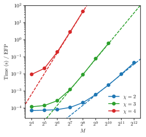
Table 4a shows the number of EFPs listed by degree $d$ and VE complexity $\chi$ (with respect to the heuristics used in our implementation), and Table 4b further breaks up the EFP counts by $N$. Fig. 1 shows the time to compute the average $d\leq 7$ EFP as a function of multiplicity $M$ for different VE complexity $\chi$. Finally, we note that though VE often provides a significant speedup over the naive algorithm, there may be even faster ways of computing the EFPs.

5 Linear regression with jet observables

Regression, classification, and generation are three dominant machine learning paradigms. Machine learning applications in collider physics have been largely focused on classification (e.g. jet tagging) Komiske:2016rsd ; Almeida:2015jua ; Baldi:2016fql ; Kasieczka:2017nvn ; Pearkes:2017hku ; Butter:2017cot ; Aguilar-Saavedra:2017rzt ; Guest:2016iqz ; Louppe:2017ipp with recent developments in regression Komiske:2017ubm and generation deOliveira:2017pjk ; Paganini:2017hrr . For a more complete review of modern machine learning techniques in jet substructure, see Ref. Larkoski:2017jix . The lack of established regression problems in jet physics is due in part to the difficulty of theoretically probing multivariate combinations as well as the challenges associated with extracting physics information from trained regressions models.

In this section, we show that the linearity of the energy flow basis mitigates many of these problems, providing a natural regression framework using simple linear models, probing the learned observable combinations, and gaining insight into the physics of the target observables. Since regression requires training samples, we observe how the regression performance compares on jets with three characteristic phase-space configurations: one-prong QCD jets, two-prong boosted $W$ jets, and three-prong boosted top jets. We use linear regression to demonstrate convergence of the energy flow basis on IRC-safe observables, while illustrating their less-performant behavior for non-IRC-safe observables.

5.1 Linear models with the energy flow basis

Linear models assume a linear relationship between the input and target variables, making them the natural choice for (machine) learning with the energy flow basis for both regression and classification. A linear model $\mathscr{M}$ with EFPs as the inputs is defined by a finite set $\mathcal{G}$ of multigraphs and numerical coefficients ${\bf w}=\{w_{G}\}_{G\in\mathcal{G}}$:

$$\mathscr{M}=\sum_{G\in\mathcal{G}}w_{G}\,\text{EFP}_{G}.$$ (75)

The fundamental relationship between EFPs, linear models, and IRC-safe observables is highlighted by comparing Eq. (75) to Eq. (5), where the linear model $\mathscr{M}$ in Eq. (75) takes the place of the IRC-safe observable $\mathcal{S}$ in Eq. (5). Because the EFPs are a complete linear basis, $\mathscr{M}$ is capable of approximating any $\mathcal{S}$ for a sufficiently large set of EFPs.

The linear structure of Eq. (75) allows for an avenue to “open the box” and interpret the learned coefficients as defining a unique multiparticle correlator for each $N$. To see this, partition the set $\mathcal{G}$ into subsets $\mathcal{G}_{N}$ of graphs with $N$ vertices. The sum in Eq. (75) can be broken into two sums, one over $N$ and the other over all graphs in $\mathcal{G}_{N}$. The linear energy structure of the EFPs in Eq. (1) allows for the second sum to be pushed inside the product of energies onto the angular weighting function:

$$\mathscr{M}=\sum_{N=0}^{N_{\rm max}}\sum_{i_{1}=1}^{M}\cdots\sum_{i_{N}=1}^{M}z_{i_{1}}\cdots z_{i_{N}}\left(\sum_{G\in\mathcal{G}_{N}}w_{G}\prod_{(k,\ell)\in G}\theta_{i_{k}i_{\ell}}\right),$$ (76)

where $N_{\rm max}$ is the maximum number of vertices of any graph in $\mathcal{G}$. The quantity in parentheses in Eq. (76) may be though of as a single angular weighting function. The linear model written in this way reveals itself to be a sum of $C$-correlators (similar to Eq. (65)), one for each $N$, where the linear coefficients within each $\mathcal{G}_{N}$ parameterize the angular weighting function $f_{N}$ of that $C$-correlator. This arrangement of the learned parameters of the linear model into $N_{\rm max}$ $C$-correlators contrasts sharply with the lack of a physical organization of parameters in nonlinear methods such as neural networks or boosted decision trees.

5.2 Event generation and EFP computation

For the studies in this section and in Sec. 6, we generate events using Pythia 8.226 Sjostrand:2006za ; Sjostrand:2007gs ; Sjostrand:2014zea with the default tunings and shower parameters at $\sqrt{s}=$13\text{\,}\mathrm{T}\mathrm{e}\mathrm{V}$$. Hadronization and multiple parton interactions (i.e. underlying event) are included, and a $400\text{\,}\mathrm{G}\mathrm{e}\mathrm{V}$ parton-level $p_{T}$ cut is applied. For quark/gluon distribution, quark (signal) jets are generated through $pp\to qZ(\to\nu\bar{\nu})$, and gluon (background) jets through $pp\to gZ(\to\nu\bar{\nu})$, where only light-quarks ($uds$) appear in the quark sample. For $W$ and top tagging, signal jets are generated through $pp\to W^{+}W^{-}(\to\text{hadrons})$ and $pp\to t\bar{t}(\to\text{hadrons})$, respectively. For both $W$ and top events, the background consists of QCD dijets.

Final state, non-neutrino particles were made massless, keeping $y$, $\phi$, and $p_{T}$ fixed, and then were clustered with FastJet 3.3.0 Cacciari:2011ma using the anti-$k_{T}$ algorithm Cacciari:2008gp with a jet radius of $R=0.4$ for quark/gluon samples and $R=0.8$ for $W$ and top samples (and the relevant dijet background). The hardest jet with rapidity $|y|<1.7$ and $500\text{ GeV}\leq p_{T}\leq 550$ GeV was kept. For each type of sample, 200k jets were generated. For the regression models, 75% were used for training and 25% for testing.

For these events, all EFPs up to degree $d\leq 7$ were computed in Python using our EnergyFlow module making use of NumPy’s einsum function. See Tables 2 and 4 for counts of EFPs tabulated by various properties such as $N$, $d$, and $\chi$. Note that all but 4 of the 1000 $d\leq 7$ EFPs can be computed in $\mathcal{O}(M^{2})$ or $\mathcal{O}(M^{3})$ in the VE paradigm, making the set of EFPs with $d\leq 7$ efficient to compute.

5.3 Spanning substructure observables with linear regression

We now consider the specific case of training linear models to approximate substructure observables with linear combinations of EFPs. For an arbitrary observable $O$, we use least-squares regression to find a suitable set of coefficients ${\bf w}^{*}$:

$${\bf w}^{*}=\underset{\bf w}{\arg\min}\left\{\sum_{J\in\text{jets}}\left(O(J)-\sum_{G\in\mathcal{G}}w_{G}\,\text{EFP}_{G}(J)\right)^{2}\right\},$$ (77)

where $O(J)$ is the value of the observable and $\text{EFP}_{G}(J)$ the value of the EFP given by multigraph $G$ on jet $J$. There are possible modifications to Eq. (77) which introduce penalties proportional to $\|{\bf w}\|_{1}$ or $\|{\bf w}\|_{2}^{2}$ where $\|\cdot\|_{1}$ is the 1-norm and $\|\cdot\|_{2}$ is the 2-norm. The first of these choices, referred to as lasso regression tibshirani1996regression , may be particularly interesting because of the variable selection behavior of this model, which would aid in selecting the most important EFPs to approximate a particular observable. We leave such investigation to future work. See Ref. bishop2006pattern for a review of linear models for regression.

We use the LinearRegression class of the scikit-learn python module scikit-learn to implement Eq. (77) with no regularization on the samples described in Sec. 5.2. In general, the smallest possible regularization which prevents overfitting (if any) should be used. Because of the linear nature of linear regression and the analytic tractability of Eq. (77), the ${\bf w}^{*}$ corresponding to the global minimum of the squared loss function can be found efficiently using convex optimization techniques. Such techniques include closed-form solutions or convergent iterative methods.

	Observable	Properties
$m_{J}$/$p_{T,J}$	Scaled jet mass	No Taylor expansion about zero energy limit
$\lambda^{(\alpha=1/2)}$	Les Houches Angularity	No analytic relationship beyond even integer $\alpha$
$\tau_{2}^{(\beta=1)}$	$2$-subjettiness	Algorithmically defined IRC-safe observable
$\tau_{21}^{(\beta=1)}$	$N$-subjettiness ratio	Sudakov safe, safe for two-prong kinematics
$\tau_{32}^{(\beta=1)}$	$N$-subjettiness ratio	Sudakov safe, safe for three-prong kinematics
$M$	Particle multiplicity	IRC unsafe

Table 5: The six substructure observables used as targets for linear regression, listed with relevant properties. The first three are IRC safe, the next two are Sudakov safe in general (and IRC safe in the noted regions of phase space), and particle multiplicity is IRC unsafe. The Les Houches Angularity Badger:2016bpw ; Gras:2017jty is calculated with respect to the $p_{T}$-weighted centroid axis in Eq. (19), and the $N$-subjettiness observables Thaler:2010tr ; Thaler:2011gf are calculated using $k_{T}$ axes.

As targets for the regression, we consider the six jet observables in Table 5 to highlight some interesting test cases. As our measure of the success of the regression, we use a variant of the correlation coefficient between the true and predicted observables that is less sensitive to outliers than the unadulterated correlation coefficient. When evaluating the trained linear model on the test set, only test samples with predicted values within the 5${}^{\text{th}}$ and 95${}^{\text{th}}$ percentiles of the predictions are included. In the contexts considered in this paper, narrowing this percentile range lowers the correlation coefficient and widening the range out toward all of the test set increases the correlation coefficient. The qualitative nature of the results are insensitive to the specific choice of percentile cutoffs. We perform this regression using EFPs of degree up to $d$ for $d$ from 2 to 7 on all three jet samples, with the results shown in Fig. 2. Histograms of the true and predicted distributions for a subset of these observables are shown in Fig. 3 for the three types of jets considered here.

(a)

(b)

(c)

Figure 2: Correlation coefficients between true and predicted values for the jet observables in Table 5, plotted as a function of maximum EFP degree. Shown are the (a) QCD dijet, (b) $W$ jet, and (c) top jet samples, and as explained in the text, we restrict to predictions in the 5${}^{\text{th}}$--95${}^{\text{th}}$ percentiles. Observables in IRC-safe regions of phase space are shown with solid lines and those in IRC-unsafe regions (including Sudakov-safe regions) are shown with dashed lines. The IRC-safe observables are all learned with correlation coefficient above 0.98 in all three cases by $d=7$. Multiplicity (black triangles) sets the scale for the regression performance on IRC-unsafe observables. Note that $\tau_{21}$ has performance similar to the IRC-safe observables only when jets are characteristically two-pronged or higher ($W$ and top jets), and similarly for $\tau_{32}$ when the jets are characteristically three-pronged (top jets).

(a)

(b)

(c)

(d)

(e)

(f)

(g)

(h)

(i)

Figure 3: The distributions of true and predicted scaled jet mass (top), $\tau_{2}^{(\beta=1)}$ (middle), and $\tau_{21}^{(\beta=1)}$ (bottom) using linear regression with EFPs up to different maximum degrees $d$ on QCD jets (left), $W$ jets (center), and top jets (right). Note the excellent agreement for the IRC-safe observables in the first two rows. Observables in IRC-safe regions of phase space are shown with solid lines and those in IRC-unsafe regions are shown with dashed lines. The Sudakov-safe $\tau_{21}^{(\beta=1)}$ predicted distributions match the true distributions for jets typically with two or more prongs ($W$ and top jets) better than for typically one-pronged (QCD) jets.

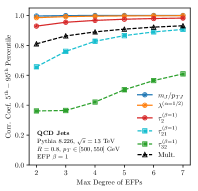
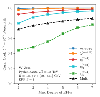
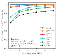
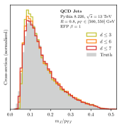
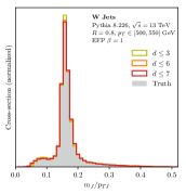
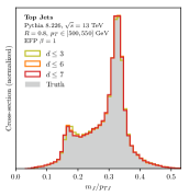
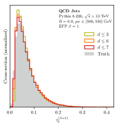
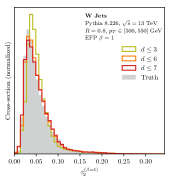
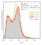
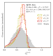
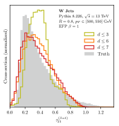
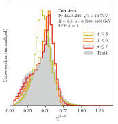
Since the learned coefficients depend on the training set, in principle different linear combinations may be learned to approximate the substructure observables in different jet contexts. This stands in contrast to the analysis in Sec. 2.3, where many jet substructure observables were identified as exact linear combinations of EFPs, independent of the choice of inputs. The IRC-safe observables---mass, Les Houches angularity, and $2$-subjettiness---are all learned with a correlation coefficient above 0.98 in all three cases by $d=7$.

The IRC-unsafe multiplicity sets the scale of performance for observables that are not IRC safe. For the $N$-subjettiness ratios, the regression performance depends on whether the observable is IRC safe or only Sudakov safe Larkoski:2013paa ; Larkoski:2015lea . The ratio $\tau_{21}$ is only IRC safe for regions of phase space with two prongs or more (i.e. the $W$ and top samples), and $\tau_{32}$ is only IRC safe for three prongs or more (i.e. just the top sample). In cases where the $N$-subjettiness ratio is IRC safe, the regression performs similarly to the other IRC-safe observables, whereas for the cases where the $N$-subjettiness ratio is only Sudakov safe, the regression performance is poor (even worse than for multiplicity). It is satisfying to see the expected behavior between the safety of the observable and the quality of the regression with EFPs.

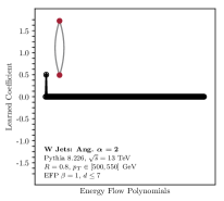
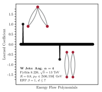
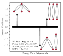
As a final cross check of the regression, we can use the linear model in Eq. (75) to confirm some of the analytic results of Sec. 2.3. Specifically, we perform a linear regression with the target observable being the even-$\alpha$ angularities with respect to the $p_{T}$-weighted centroid axis. These were shown to be non-trivial linear combinations of EFPs in Sec. 2.3.3. Regressing onto $\lambda^{(2)},\,\lambda^{(4)},$ and $\lambda^{(6)}$, the linear model learned the observables with effectively 100% accuracy and the learned linear combination was exactly that predicted by Eqs. (21), (24), and (29), up to a precision of $10^{-6}$. Fig. 4 shows the learned linear combinations of EFPs for the $W$ jet sample.

(a)

(b)

(c)

Figure 4: The linear combinations of EFPs learned by linear regression for even-$\alpha$ angularities with the $W$ jet samples. Shown are (a) $\alpha=2$, (b) $\alpha=4$, and (c) $\alpha=6$. All but the highlighted EFP coefficients are learned to be near zero. The EFPs corresponding to those non-zero coefficients are illustrated directly on the figure. The learned linear coefficients are exactly those predicted analytically in Eqs. (21), (24), and (29). The same behavior is found with the QCD and top jet samples.

6 Linear jet tagging

We now apply the energy flow basis to three representative jet tagging problems---light-quark/gluon classification, $W$ tagging, and top tagging---providing a broad set of contexts in which to study the EFPs. Since the energy flow basis is linear, we can (in principle) access the optimal IRC-safe observable for jet tagging by training a linear classifier for this problem. As mentioned in Sec. 5.3, one benefit of linear models, in addition to their inherent simplicity, is that they are typically convex problems which can be solved exactly or with gradient descent to a global minimum. See Ref. bishop2006pattern for a review of linear models for classification.

A (binary) linear classifier learns a vector ${\bf w}^{*}$ that defines a hyperplane orthogonal to the vector. A bias term, which can be related to the distance of this hyperplane from the origin, sets the location of the decision boundary, which is the hyperplane translated away from the origin. The decision function for a particular point in the input space is the normal distance to the decision boundary. In contrast with regression, where the target variable is usually continuous, classification predictions are classes, typically 0 or 1 for a binary classifier.

Different methods of determining the vector ${\bf w}^{*}$---such as logistic regression, support vector machines, or linear discriminant analysis---may learn different linear classifiers since the methods optimize different loss functions. For our linear classifier, we use Fisher’s linear discriminant fisher1936use provided by the LinearDiscriminantAnalysis class of the scikit-learn python module scikit-learn . The choice of logistic regression was also explored, and jet tagging performance was found to be insensitive to which type of linear classifier was used.

The details of the event generation and EFP computation are the same as in Sec. 5.2. To avoid a proliferation of plots, we present only the case of $W$ tagging in the text and refer to App. B for the corresponding results for quark/gluon discrimination and top tagging. Qualitatively similar results are obtained on all three tagging problems, with the conclusion that linear classification with EFPs yields comparable classification performance to other powerful machine learning techniques. This is good evidence that the EFPs provides a suitable linear expansion of generic IRC-safe information relevant for practical jet substructure applications.

6.1 Alternative jet representations

In order to benchmark the EFPs, we compare them to two alternative jet tagging paradigms:

• The jet images approach Cogan:2014oua treats calorimeter deposits as pixels and the jet as an image, often using convolutional neural networks to determine a classifier. Jet images have been applied successfully to the same tagging problems considered here: quark/gluon discrimination Komiske:2016rsd , $W$ tagging deOliveira:2015xxd , and top tagging Kasieczka:2017nvn ; Baldi:2016fql .

• The $\boldsymbol{N}$-subjettiness basis was introduced for $W$ tagging in Ref. Datta:2017rhs and later applied to tagging non-QCD jets Aguilar-Saavedra:2017rzt . We use the same choice of $N$-subjettiness basis elements as Ref. Datta:2017rhs , namely:

  $$\{\tau_{1}^{(1/2)},\tau_{1}^{(1)},\tau_{1}^{(2)},\tau_{2}^{(1/2)},\tau_{2}^{(1)},\tau_{2}^{(2)},\cdots,\tau_{N-2}^{(1/2)},\tau_{N-2}^{(1)},\tau_{N-2}^{(2)},\tau_{N-1}^{(1)},\tau_{N-1}^{(2)}\},$$ (78)

  with $3N-4$ elements needed to probe $N$-body phase space. These are then used as inputs to a DNN.

Both of these learning paradigms are expected to perform well, and we will see below that this is the case. As a strawman, we also consider linear classification with the $N$-subjettiness basis elements in Eq. (78), which is not expected to yield good performance. For completeness, we also perform DNN classification with the energy flow basis.

We now summarize the technical details of these alternative jet tagging approaches. For jet images, we create $33\times 33$ jet images spanning $2R\times 2R$ in the rapidity-azimuth plane. Motivated by Ref. Komiske:2016rsd , both single-channel ‘‘grayscale’’ jet images of the $p_{T}$ per pixel and two-channel ‘‘color’’ jet images consisting of the $p_{T}$ channel and particle multiplicity per pixel were used. The $p_{T}$-channel of the jet image was normalized such that the sum of the pixels was one. Standardization was used to ensure that each pixel had zero mean and unit standard deviation by subtracting the training set mean and dividing by the training set standard deviation of each pixel in each channel. A jet image CNN architecture similar to that used in Ref. Komiske:2016rsd was employed: three 36-filter convolutional layers with filter sizes of $8\times 8$, $4\times 4$, and $4\times 4$, respectively, followed by a 128-unit dense layer and a 2-unit softmaxed output. A rectified linear unit (ReLU) activation nair2010rectified was applied to the output of each internal layer. Maxpooling of size $2\times 2$ was performed after each convolutional layer with a stride length of 2. The dropout rate was taken to be 0.1 for all layers. He-uniform initialization heuniform was used to initialize the model weights.

For the DNN (both for the $N$-subjettiness basis and for the EFPs), we use an architecture consisting of three dense layers of 100 units each connected to a 2-unit softmax output layer, with ReLU activation functions applied to the output of each internal layer. For the training of all networks, 300k samples were used for training, 50k for validation, and 50k for testing. Networks were trained using the Adam algorithm adam using categorical cross-entropy as a loss function with a learning rate of $10^{-3}$ and a batch size of 100 over a maximum of 50 epochs. Early stopping was employed, monitoring the validation loss, with a patience parameter of 5. The python deep learning library Keras keras with the Theano backend bergstra2010theano was used to instantiate and train all neural networks. Training of the CNNs was performed on Microsoft Azure using NVIDIA Tesla K80 GPUs and the NVIDIA CUDA framework. Neural network performance was checked to be mildly insensitive to these parameter choices, but these parameter choices were not tuned for optimality. As a general rule, the neural networks used here are employed to give a sense of scale for the performance attainable with jet images and the $N$-subjettiness basis using out-of-the-box techniques; improvements in classification accuracy may be possible for these methods with additional hyperparameter tuning.

6.2 $W$ tagging results and comparisons

We present results for the $W$ tagging study here, with the other two classification problems discussed in App. B. The performance of a binary classifier is encapsulated by the background mistag rate $\varepsilon_{b}$ at a given signal efficiency $\varepsilon_{s}$. For all of the figures below, we plot inverse receiver operator characteristic (ROC) curves, $1/\varepsilon_{b}$ as a function of $\varepsilon_{s}$, on a semi-log scale; a higher ROC curve indicates a better classifier. The corresponding standard ROC ($\varepsilon_{b}$ vs. $\varepsilon_{s}$) and significance improvement ($\varepsilon_{s}/\sqrt{\varepsilon_{b}}$ vs. $\varepsilon_{s}$) curves are available in the source files of the arXiv preprint as additional pages in the figure.

Figure 5: Inverse ROC curves for linear $W$ tagging with the energy flow basis using different choices of angular exponent $\beta$ in Eq. (11). Though the improvement is mild, $\beta=0.5$ shows the best overall performance. See Fig. 10 for the corresponding quark/gluon discrimination and top tagging results, where $\beta=0.5$ is also the best choice by a slight margin.

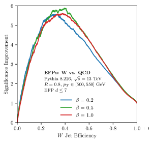
We begin by studying the performance for different choices of angular exponent $\beta$ in the default hadronic measure from Eq. (11). Fig. 5 shows ROC curves for the choices of $\beta=0.2$, $\beta=0.5$, and $\beta=1$, using all EFPs with $d\leq 7$. The differences in performance are mild, but $\beta=0.5$ slightly improves the ROC curves for $W$ tagging, so we use $\beta=0.5$ for the remainder of our studies. The choice of $\beta=0.5$ was also found to be optimal for the cases of quark/gluon and top tagging discussed in App. B.

(a)

(b)

Figure 6: Inverse ROC curves for $W$ tagging with (a) the energy flow basis including degrees up to $d=7$ and (b) the $N$-subjettiness basis up to 10-body phase space information. In both cases, we show the observables combined linearly (solid) and with a DNN (dashed). The linear combinations of EFPs can be seen to approach the nonlinear combinations, particularly for higher signal efficiencies, while the linear combinations of the $N$-subjettiness basis can be seen to saturate well below the nonlinear combinations as the number of observables is increased. See Fig. 11 for the corresponding quark/gluon discrimination and top tagging results.

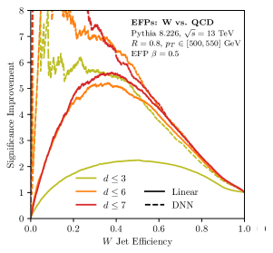
Next, in Fig. 6a, we test the linear spanning nature of the EFPs by comparing the ROC curves of the linear and nonlinear models trained on EFPs up to different $d$. With linear regression, there is a large jump in performance in going from $d\leq 3$ (13 EFPs) to $d\leq 6$ (314 EFPs), and a slight increase in performance from $d\leq 6$ to $d\leq 7$ (1000 EFPs), indicating good convergence to the optimal IRC-safe observable for $W$ jet discrimination. To avoid cluttering the plot, $d\leq 4$ and $d\leq 5$ are not shown in Fig. 6a, but their ROC curves fall between those of $d\leq 3$ and $d\leq 6$, highlighting that the higher $d$ EFPs carry essential information for linear classification. By contrast, using nonlinear classification with a DNN, the EFPs performance with $d\leq 3$ is already very good, since functions of the low $d$ EFPs can be combined in a nonlinear fashion to construct information contained in higher $d$ composite EFPs. The linear and nonlinear performance is similar with the $d\leq 7$ EFPs for operating points of $\varepsilon_{s}\gtrsim 0.5$, though the nonlinear DNN outperforms the linear classifier in the low signal efficiency region. It should be noted that the linear classifier is not trained specifically for the low signal efficiency region and it may be possible that choosing a different hyperplane could boost performance there. We leave to future work a more detailed investigation of optimizing the choice of linear classifier.

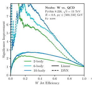
The performance of the $N$-subjettiness basis with both linear and nonlinear classifiers is shown in Fig. 6b. For both linear classification and the DNN, performance appears to saturate with the 6-body (14 $\tau_{N}$s) phase space, with not much gained in going to 10-body (26 $\tau_{N}$s) phase space, except for a small increase in the low signal efficiency region for the DNN; we confirmed up to 30-body (86 $\tau_{N}$s) phase space that no change in ROC curves was observed compared to 10-body phase space. As expected, there is relativity poor performance with linear classification even as the dimension of phase space is increased. Classification with a DNN, though, shows an immense increase in performance over linear classification, as expected since the $N$-subjettiness basis is expected to nonlinearly capture all of the relevant IRC-safe kinematic information Datta:2017rhs . This illustrates that nonlinear combinations of the $N$-subjettiness observables are crucial for extracting the full physics information.

The corresponding quark/gluon and top tagging plots in Fig. 11 effectively tell the same story as Fig. 6, robustly demonstrating the linear spanning nature of the EFPs used for classification across a wide variety of kinematic configurations. As a side note, in App. B there are sometimes cases where a linear combination of EFPs yields improved performance compared to a DNN on the same inputs, particularly at medium to high signal efficiencies. Since even a one-node DNN should theoretically be able to learn the linear combination of EFPs learned by the linear classifier, regimes where the linear classifier outperforms the DNN demonstrate the inherent difficulty of training complex multivariate models.

Figure 7: Inverse ROC curves for $W$ tagging comparing six different methods: linear and DNN classification with the energy flow basis up to $d\leq 7$, linear and DNN classification with the $N$-subjettiness basis up to 10-body phase space, and grayscale and color jet images with CNNs. The most evident gap is between the linearly-combined $N$-subjettiness basis and the remaining curves, which achieve similar classification performance for medium and high signal efficiencies. See Fig. 12 for the corresponding quark/gluon discrimination and top tagging results.

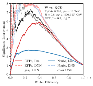
In Fig. 7 we directly compare the EFP classification power against the $N$-subjettiness basis and the 1-channel (‘‘grayscale’’) and 2-channel (‘‘color’’) CNNs. For operating points with $\varepsilon_{s}\gtrsim 0.5$, all methods except the linear $N$-subjettiness classifier show essentially the same performance. The worse performance of the linear EFP classifier at low signal efficiencies is expected, since the Fisher linear discriminant is not optimized for that regime. Overall, it is remarkable that similar classification performance can be achieved with these three very different learning paradigms, especially considering that the DNNs and grayscale CNN implicitly, and the color CNN explicitly, have access to non-IRC-safe information (including Sudakov-safe combinations of the IRC-safe inputs). This agreement gives evidence that the tagging techniques have approached a global bound on the maximum possible discrimination power achievable, at least in the context of parton shower simulations.

Once again, the analogous quark/gluon and top tagging plots, shown in Fig. 12, show very similar behavior to the $W$ tagging case in Fig. 7. Linear classification with the EFPs performs similarly to the DNNs and CNNs, tending to slightly outperform at high signal efficiencies and underperform at low signal efficiencies. Ultimately, the choice of tagging method comes down to a trade off between the simplicity of the inputs and the simplicity of the training method, with the EFPs presently requiring more inputs than the $N$-subjettiness basis but with the benefit of using a linear model. In the future, we plan to study ways of reducing the size of the EFP basis by exploiting linear redundancies among the EFPs and using powerful linear methods to automatically select the most important observables for a given task.

6.3 Opening the energy flow box

(a)

(b)

Figure 8: Inverse ROC curves for linear $W$ tagging with the energy flow basis with $d\leq 7$, sweeping over (a) which $N$-point correlators and (b) observables of which VE computational complexity $\mathcal{O}(M^{\chi})$ are included in the linear fit. It is clear that important information is contained in the higher $N$-particle correlators, which can be included because the algorithm in Sec. 4 evades the naive $\mathcal{O}(M^{N})$ scaling. Interestingly, the discrimination power appears to be almost saturated by the graphs computable in $\mathcal{O}(M^{2})$. See Fig. 13 for the corresponding quark/gluon discrimination and top tagging results.

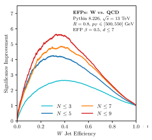
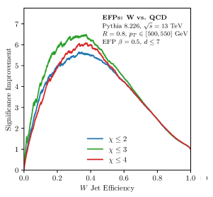
As argued in Eq. (76), one of the main advantages of linear methods with the energy flow basis is that one can attempt to ‘‘open the box’’ and directly explore what features have been learned. We leave to future work a full exploration of this possibility, but here we attempt to probe which topological structures within the EFP basis carry the discrimination power for the different tagging problems. Since we have shown that the EFPs with $d\leq 7$ have sufficient discrimination power to qualitatively match the performance of alternative tagging methods, we will restrict to this set of observables.

In Fig. 8a, we vary the maximum number of vertices in the EFP graphs, where the maximum $N$ is $14$ for $d\leq 7$, finding that the performance roughly saturates at $N=9$, highlighting the importance of higher $N$ EFPs. The algorithmic advances described in Sec. 4 allow for the efficient computation of these higher $N$ EFPs, which have complexities as intractable as $\mathcal{O}(M^{9})$ with the naive algorithm. Additionally, note that nearly every EFP (all except those corresponding to complete graphs) has a non-vanishing angular weighting function, which is a new feature compared to the ECFs and ECFGs (see Sec. 2.4). In Fig. 8b, we vary the maximum computational complexity $\chi$ of the EFP graphs, where the maximum $\chi$ is $4$ for $d\leq 7$. Remarkably, the full performance of linear classification with the $d\leq 7$ EFPs can be obtained with merely those observables calculable in $\mathcal{O}(M^{2})$ with VE. Thus, fortuitously for the purposes of jet tagging, it seems that restricting to the most efficiently computable EFPs (in the VE paradigm) is sufficient for extracting the near-optimal IRC-safe observable for jet discrimination. Similar results hold for quark/gluon discrimination and top tagging, shown in Fig. 13.

7 Conclusions

In this paper, we have introduced the EFPs, which linearly span the space of IRC-safe observables. The core argument, presented in Sec. 3, is that one can systematically expand an arbitrary IRC-safe observable in terms of energies and angles and read off the unique resulting analytic structures. This expansion yields a new way to understand the importance of $C$-correlators Tkachov:1995kk ; Sveshnikov:1995vi ; Cherzor:1997ak ; Tkachov:1999py for IRC safety, and it enables a powerful graph-theoretic representation of the various angular structures. The multigraph correspondence makes manifest a more efficient algorithm than the naive $\mathcal{O}(M^{N})$ one for computing EFPs, overcoming a primary obstacle to exploring higher-$N$ multiparticle correlators for jet substructure.

To demonstrate the power of the energy flow basis, we performed a variety of representative regression and classification tasks for jet substructure. Crucially, linear methods were sufficient to achieve good performance with the EFPs. As a not-quite apples-to-apples comparison in three representative jet tagging applications, linear classification with 1000 EFPs achieved comparable performance to a CNN acting on a jet image with $33\times 33=1089$ pixels. Because of the wide variety of linear learning methods available bishop2006pattern , we expect that the EFPs will be a useful starting point to explore more applications in jet substructure and potentially elsewhere in collider physics.

There are many possible refinements and extensions to the energy flow basis. In this paper, we truncated the EFPs at a fixed maximum degree $d$; alternatively, one could truncate the prime EFPs at a fixed $d$ and compute all composite EFPs up to a specified cutoff. Since the EFPs yield an overcomplete basis, it could be valuable to cull the list of required multigraphs. A similar problem of overcompleteness was solved for kinematic polynomial rings in Ref. Henning:2017fpj , and that strategy may be relevant for EFPs with a suitable choice of measure. In the other direction, it may be valuable to make the energy flow basis even more redundant by including EFPs with multiple measures. With a vastly overcomplete basis, one could use techniques like lasso regression tibshirani1996regression to zero out unnecessary terms. While we have restricted our attention to IRC-safe observables, it would be straightforward to relax the restriction to just infrared safety. In particular, the set of IR-safe (but C-unsafe) functions in Eq. (3.1.3) can be expanded into multigraphs that have an extra integer decoration on each vertex to indicate the energy scaling. Finally, the EFPs are based on an expansion in pairwise angles, but one could explore alternative angular expansions in terms of single particle directions or multiparticle factors.

To gain some perspective, we find it useful to discuss the EFPs in the broader context of machine learning for jet substructure. Over the past few years, there has been a surge of interest in using powerful tools from machine learning to learn useful observables from low-level or high-level representations of a jet Cogan:2014oua ; deOliveira:2015xxd ; Komiske:2016rsd ; Almeida:2015jua ; Baldi:2016fql ; Kasieczka:2017nvn ; Pearkes:2017hku ; Butter:2017cot ; Aguilar-Saavedra:2017rzt ; Guest:2016iqz ; Louppe:2017ipp ; Datta:2017rhs ; Baldi:2014kfa ; Baldi:2014pta ; Gallicchio:2010dq ; Gallicchio:2012ez ; Gallicchio:2011xq . The power of these machine learning methods is formidable, and techniques like neural networks and boosted decision trees have shifted the focus away from single- or few-variable jet substructure taggers to multivariate methods. On the other hand, multivariate methods can sometimes obscure the specific physics information that the model learns, leading to recent efforts to ‘‘open the box’’ of machine learning tools deOliveira:2015xxd ; Butter:2017cot ; Chang:2017kvc ; Komiske:2017ubm ; Metodiev:2018ftz . Even with an open box, though, theoretical calculations of multivariate distributions are impractical (if not impossible). Furthermore, training multivariate models is often difficult, requiring large datasets, hyperparameter tuning, and preprocessing of the data.

The EFPs represent both a continuation of and a break from these machine learning trends. The EFPs continue the trend from multivariate to hypervariate representations for jet information, with $\mathcal{O}(100)$ elements needed for effective regression and classification. On the other hand, the linear-spanning nature of the EFPs make it feasible to move away from ‘‘black box’’ nonlinear algorithms and return to simpler linear methods (explored previously for jet substructure in e.g. Thaler:2011gf ; Cogan:2014oua ) without loss of generality. Armed with the energy flow basis, there is a suite of powerful tools and ideas from linear regression and classification which can now be fully utilized for jet substructure applications, with simpler training processes compared to DNNs and stronger guarantees of optimal training convergence. Multivariate methods would ideally be trained directly on data to avoid relying on imperfect simulations, as discussed in Ref. Komiske:2018oaa . The energy flow basis may be compelling for recent data-driven learning approaches Komiske:2018oaa ; Dery:2017fap ; Metodiev:2017vrx due to its completeness, the simplicity of linear learning algorithms, and a potentially lessened requirement on the size of training samples.

As with any jet observable, the impact of non-perturbative effects on the EFPs is important to understand. Even with IRC safety, hadronization modifies the distributions predicted by pQCD and therefore complicates first-principles calculations. It would be interesting to see if the shape function formalism Korchemsky:1999kt ; Korchemsky:2000kp could be used to predict the impact of non-perturbative contributions to EFP distributions. Alternatively, one standard tool that is used to mitigate non-perturbative effects is jet grooming Butterworth:2008iy ; Ellis:2009su ; Ellis:2009me ; Krohn:2009th ; Dasgupta:2013ihk ; Larkoski:2014wba , which also simplifies first-principles calculations and allows for ‘‘quark’’ and ‘‘gluon’’ jets to be theoretically well-defined Frye:2016aiz . We leave a detailed study of the effects of non-perturbative contributions and jet grooming on EFPs to future work.

Eventually, one hopes that the EFPs will be amenable to precision theoretical calculations of jet substructure (see e.g. Refs. Feige:2012vc ; Dasgupta:2013ihk ; Dasgupta:2013via ; Larkoski:2014tva ; Procura:2014cba ; Larkoski:2015kga ; Dasgupta:2015lxh ; Frye:2016aiz ; Dasgupta:2016ktv ; Marzani:2017mva ; Larkoski:2017cqq ). This is by no means obvious, since generic EFPs have different power-counting structures from the ECFs Larkoski:2013eya or ECFGs Moult:2016cvt . That said, phrasing jet substructure entirely in the language of energy flow observables and energy correlations may provide interesting new theoretical avenues to probe QCD, realizing the $C$-correlator vision of Refs. Tkachov:1995kk ; Sveshnikov:1995vi ; Cherzor:1997ak ; Tkachov:1999py . Most IRC-safe jet observables rely on particle-level definitions and calculations, but there has been theoretical interest in directly analyzing the correlations of energy flow in specific angular directions basham1978energy ; basham1979energy ; Belitsky:2001ij , particularly in the context of conformal field theory Hofman:2008ar ; Engelund:2012re ; Zhiboedov:2013opa ; Belitsky:2013xxa ; Belitsky:2013bja . The energy flow basis is a step towards connecting the particle-level and energy-correlation pictures, and one could even imagine that the energy flow logic could be applied directly at the path integral level. Ultimately, the structure of the EFPs is a direct consequence of IRC safety, resulting in a practical tool for jet substructure at colliders as well as a new way of thinking about the space of observables more generally.

Appendix A Energy flow and the stress-energy tensor

Figure 9: An example calorimeter cell configuration to measure a 5-point energy correlator. The red regions indicate the five calorimeter cells chosen to measure the energy infinitely far from the interaction. For each event, the values of the five energy deposits are multiplied together to obtain the value of the observable in Eq. (81).

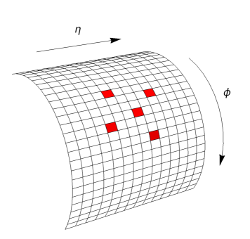
In this appendix, we review the connection between the energy flow of an event, as described by the stress-energy tensor, to multiparticle energy correlators Tkachov:1995kk ; Sveshnikov:1995vi ; Cherzor:1997ak ; Tkachov:1999py .

Consider an idealized hadronic calorimeter cell at position $\hat{n}$ in pseudorapidity-azimuth $(\eta,\phi)$-space, spanning a patch of size $d\eta\,d\phi$. The energy flow operator $\mathcal{E}_{T}(\hat{n})$ corresponding to the total transverse momentum density flowing into the calorimeter cell can be written in terms of the stress-energy tensor $T_{\mu\nu}$ Sveshnikov:1995vi ; Korchemsky:1997sy ; Lee:2006nr ; Bauer:2008dt ; Mateu:2012nk as:

$$\mathcal{E}_{T}(\hat{n})=\frac{1}{\cosh^{3}\eta}\lim_{R\to\infty}R^{2}\int_{0}^{\infty}dt\,\hat{n}_{i}\,T^{0i}(t,R\hat{n}),$$ (79)

with its action on a state $\ket{X}$ of $M$ massless particles given by:

$$\mathcal{E}_{T}(\hat{n})\ket{X}=\sum_{i\in X}p_{T,i}\delta(\eta-\eta_{i})\delta(\phi-\phi_{i})\ket{X}.$$ (80)

Next, consider $N$ calorimeter cells at positions $(\hat{n}_{1},\cdots,\hat{n}_{N})$. An illustration of an example calorimeter cell configuration is shown in Fig. 9. For an event $X$, multiply together the measured energy deposits in each of these $N$ cells. The corresponding observable is then the energy $N$-point correlator as defined in Refs. basham1978energy ; basham1979energy :

$$\mathcal{E}_{T}(\hat{n}_{1})\cdots\mathcal{E}_{T}(\hat{n}_{N})\ket{X}=\sum_{i_{1}\in X}\cdots\sum_{i_{N}\in X}\left[\prod_{j=1}^{N}p_{T,i_{j}}\delta^{2}(\hat{n}_{j}-\hat{p}_{i_{j}})\right]\ket{X},$$ (81)

where $\hat{n}_{a}=(\eta_{a},\phi_{a})$ for the calorimeters cells and $\hat{p}_{a}=(\eta_{a},\phi_{a})$ for the particles in the event.

We can define a new set of observables in terms of the $N$-point correlators in Eq. (81). Consider averaging Eq. (81) over all calorimeter cells with an arbitrary angular weighting function $f_{N}(\hat{n}_{1},\ldots,\hat{n}_{N})$. The resulting observables are then of the form:

$$\mathcal{C}_{N}^{f_{N}}\ket{X} =\int d^{2}\hat{n}_{1}\cdots d^{2}\hat{n}_{N}\,f_{N}(\hat{n}_{1},\ldots,\hat{n}_{N})\mathcal{E}_{T}(\hat{n}_{1})\cdots\mathcal{E}_{T}(\hat{n}_{N})\ket{X}$$ (82)

$$=\sum_{i_{1}\in X}\cdots\sum_{i_{N}\in X}p_{T,i_{1}}\cdots p_{T,i_{N}}f_{N}(\hat{p}_{i_{1}},\ldots,\hat{p}_{i_{N}})\ket{X},$$ (83)

namely, these observables $\mathcal{C}_{N}^{f_{N}}$ written in the form of Eq. (83) are exactly the $C$-correlators defined in Eq. (3). Thus the averaging process of Eq. (82) relates the particle-level $C$-correlators of Eq. (3) to the energy flow of the stress-energy tensor $T_{\mu\nu}$.

Appendix B Quark/gluon discrimination and top tagging results

(a)

(b)

Figure 10: Same as Fig. 5, but for (a) quark/gluon discrimination and (b) top tagging. Similar to the $W$ tagging case, the $\beta=0.5$ choice has the best performance (marginally) for both tagging problems.

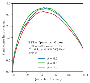
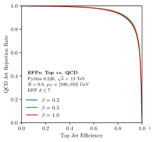
In this appendix, we supplement the $W$ tagging results of Sec. 6 with the corresponding results for quark/gluon discrimination and top tagging. The details of the event generation are given in Sec. 5.2.

We compare the EFP linear classification performance with $\beta=0.2$, $\beta=0.5$, and $\beta=1$ in Fig. 10. Consistent with the $W$ tagging case in Fig. 5, we find that the optimal performance is achieved with $\beta=0.5$. We therefore use $\beta=0.5$ for the remainder of this study.

(a)

(b)

(c)

(d)

Figure 11: Same as Fig. 6, but for quark/gluon discrimination (top) and top tagging (bottom). As in the $W$ tagging case, the linear combinations of EFPs can be seen to approach (or even exceed) the nonlinear combinations, particularly for higher signal efficiencies.

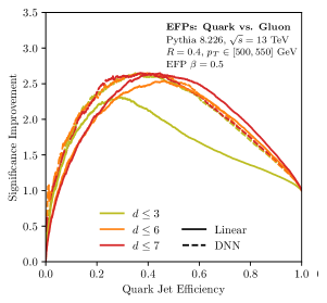
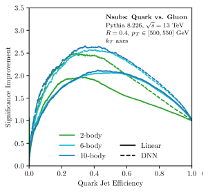
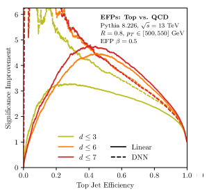
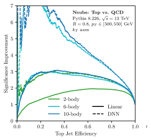
In Fig. 11 we compare the linear and nonlinear performances of the energy flow basis and the $N$-subjettiness basis. There is a clear gap between the linear and nonlinear $N$-subjettiness classifiers, whereas no such gap exists for the EFPs. Interestingly, the linear classifier of EFPs tends to outperform the DNN at medium and high signal efficiencies, indicating the difficulty of training high-dimensional neural networks. This behavior was not seen in Fig. 6, most likely because the achievable efficiency is overall higher in the $W$ tagging case.

(a)

(b)

Figure 12: Same as Fig. 7 for (a) quark/gluon discrimination and (b) top tagging. As in the $W$ tagging case, the linear classification with EFPs can match (or even outperform) the other methods at high signal efficiencies.

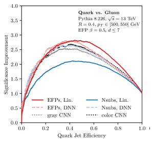
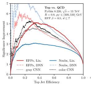
A summary of the six tagging methods is shown in Fig. 12, comparing linear and nonlinear combinations of the energy flow basis and $N$-subjettiness basis to grayscale and color jet images. As in Fig. 7, linear combinations of EFP tend to match or outperform the other methods, especially at high signal efficiencies.

(a)

(b)

(c)

(d)

Figure 13: Same as Fig. 8 but for (top) quark/gluon discrimination and (bottom) top tagging.

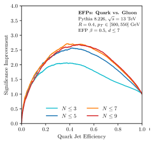
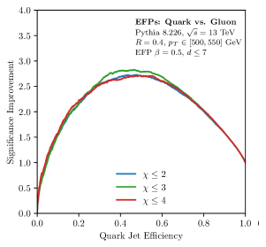
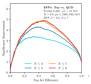
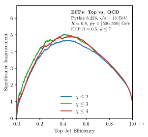
Finally, we truncate the set of EFPs with $d\leq 7$ by the number of vertices $N$ and by the VE computational complexity $\chi$ in Fig. 13. As in Fig. 8, the higher $N$-particle correlators contribute to the classification performance up to at least $N=7$, whereas the higher-complexity EFPs beyond $\chi=2$ do not significantly contribute to the classification performance.

References

- (1) M. H. Seymour, Tagging a heavy Higgs boson, in ECFA Large Hadron Collider Workshop, Aachen, Germany, 4-9 Oct 1990: Proceedings.2., pp. 557--569, 1991.
- (2) M. H. Seymour, Searches for new particles using cone and cluster jet algorithms: A Comparative study, Z. Phys. C62 (1994) 127--138.
- (3) J. M. Butterworth, B. E. Cox and J. R. Forshaw, scattering at the CERN LHC, Phys. Rev. D65 (2002) 096014, [hep-ph/0201098].
- (4) J. M. Butterworth, J. R. Ellis and A. R. Raklev, Reconstructing sparticle mass spectra using hadronic decays, JHEP 05 (2007) 033, [hep-ph/0702150].
- (5) J. M. Butterworth, A. R. Davison, M. Rubin and G. P. Salam, Jet substructure as a new Higgs search channel at the LHC, Phys. Rev. Lett. 100 (2008) 242001, [0802.2470].
- (6) CMS collaboration, S. Chatrchyan et al., Search for a Higgs boson in the decay channel to ZZ(*) to qbar l+ in collisions at TeV, JHEP 04 (2012) 036, [1202.1416].
- (7) CMS collaboration, Search for a Standard Model-like Higgs boson decaying into WW to l nu qqbar in pp collisions at sqrt s = 8 TeV, Tech. Rep. CMS-PAS-HIG-13-008, 2013.
- (8) ATLAS collaboration, G. Aad et al., Measurement of colour flow with the jet pull angle in events using the ATLAS detector at TeV, Phys. Lett. B750 (2015) 475--493, [1506.05629].
- (9) ATLAS collaboration, G. Aad et al., Measurement of jet charge in dijet events from =8 TeV pp collisions with the ATLAS detector, Phys. Rev. D93 (2016) 052003, [1509.05190].
- (10) Performance of jet substructure techniques in early TeV collisions with the ATLAS detector, Tech. Rep. ATLAS-CONF-2015-035, 2015.
- (11) ATLAS collaboration, G. Aad et al., Measurement of the differential cross-section of highly boosted top quarks as a function of their transverse momentum in = 8 TeV proton-proton collisions using the ATLAS detector, Phys. Rev. D93 (2016) 032009, [1510.03818].
- (12) ATLAS collaboration, G. Aad et al., Identification of boosted, hadronically decaying W bosons and comparisons with ATLAS data taken at TeV, Eur. Phys. J. C76 (2016) 154, [1510.05821].
- (13) ATLAS collaboration, Studies of -tagging performance and jet substructure in a high rich sample of large- jets from collisions at TeV with the ATLAS detector, Tech. Rep. ATLAS-CONF-2016-002, 2016.
- (14) ATLAS collaboration, Boosted Higgs () Boson Identification with the ATLAS Detector at TeV, Tech. Rep. ATLAS-CONF-2016-039, 2016.
- (15) ATLAS collaboration, Discrimination of Light Quark and Gluon Jets in collisions at TeV with the ATLAS Detector, Tech. Rep. ATLAS-CONF-2016-034, 2016.
- (16) CMS collaboration, Measurement of the production cross section at 13 TeV in the all-jets final state, Tech. Rep. CMS-PAS-TOP-16-013, 2016.
- (17) ATLAS, CMS collaboration, G. Rauco, Distinguishing quark and gluon jets at the LHC, in Proceedings, Parton Radiation and Fragmentation from LHC to FCC-ee: CERN, Geneva, Switzerland, November 22-23, 2016.
- (18) ATLAS collaboration, Performance of Top Quark and W Boson Tagging in Run 2 with ATLAS, Tech. Rep. ATLAS-CONF-2017-064, 2017.
- (19) CMS collaboration, A. M. Sirunyan et al., Inclusive search for a highly boosted Higgs boson decaying to a bottom quark-antiquark pair, Phys. Rev. Lett. 120 (2018) 071802, [1709.05543].
- (20) CMS collaboration, Search for BSM Production in the Boosted All-Hadronic Final State, Tech. Rep. CMS-PAS-EXO-11-006, 2011.
- (21) CMS collaboration, S. Chatrchyan et al., Search for Anomalous Production in the Highly-Boosted All-Hadronic Final State, JHEP 09 (2012) 029, [1204.2488].
- (22) ATLAS, CMS collaboration, S. Fleischmann, Boosted top quark techniques and searches for resonances at the LHC, J. Phys. Conf. Ser. 452 (2013) 012034.
- (23) ATLAS, CMS collaboration, J. Pilot, Boosted Top Quarks, Top Pair Resonances, and Top Partner Searches at the LHC, EPJ Web Conf. 60 (2013) 09003.
- (24) ATLAS collaboration, T. A. collaboration, Performance of boosted top quark identification in 2012 ATLAS data, Tech. Rep. ATLAS-CONF-2013-084, 2013.
- (25) CMS collaboration, Search for pair-produced vector-like quarks of charge -1/3 decaying to bH using boosted Higgs jet-tagging in pp collisions at sqrt(s) = 8 TeV, Tech. Rep. CMS-PAS-B2G-14-001, 2014.
- (26) CMS collaboration, Search for top-Higgs resonances in all-hadronic final states using jet substructure methods, Tech. Rep. CMS-PAS-B2G-14-002, 2014.
- (27) CMS collaboration, V. Khachatryan et al., Search for vector-like T quarks decaying to top quarks and Higgs bosons in the all-hadronic channel using jet substructure, JHEP 06 (2015) 080, [1503.01952].
- (28) ATLAS collaboration, Search for diboson resonances in the final state in collisions at 13 TeV with the ATLAS detector, Tech. Rep. ATLAS-CONF-2015-068, 2015.
- (29) ATLAS collaboration, Search for diboson resonances in the llqq final state in pp collisions at = 13 TeV with the ATLAS detector, Tech. Rep. ATLAS-CONF-2015-071, 2015.
- (30) CMS collaboration, V. Khachatryan et al., Search for a massive resonance decaying into a Higgs boson and a W or Z boson in hadronic final states in proton-proton collisions at TeV, JHEP 02 (2016) 145, [1506.01443].
- (31) CMS collaboration, Search for production in the decay channel with pp collisions at the CMS experiment, Tech. Rep. CMS-PAS-HIG-16-004, 2016.
- (32) CMS collaboration, Search for dark matter in association with a boosted top quark in the all hadronic final state, Tech. Rep. CMS-PAS-EXO-16-017, 2016.
- (33) CMS collaboration, Search for top quark-antiquark resonances in the all-hadronic final state at sqrt(s)=13 TeV, Tech. Rep. CMS-PAS-B2G-15-003, 2016.
- (34) CMS collaboration, Searches for invisible Higgs boson decays with the CMS detector., Tech. Rep. CMS-PAS-HIG-16-016, 2016.
- (35) ATLAS collaboration, M. Aaboud et al., Searches for heavy diboson resonances in collisions at TeV with the ATLAS detector, JHEP 09 (2016) 173, [1606.04833].
- (36) CMS collaboration, V. Khachatryan et al., Search for dark matter in proton-proton collisions at 8 TeV with missing transverse momentum and vector boson tagged jets, JHEP 12 (2016) 083, [1607.05764].
- (37) CMS collaboration, Search for new physics in a boosted hadronic monotop final state using of data, Tech. Rep. CMS-PAS-EXO-16-040, 2016.
- (38) CMS collaboration, Search for dark matter in final states with an energetic jet, or a hadronically decaying W or Z boson using of data at , Tech. Rep. CMS-PAS-EXO-16-037, 2016.
- (39) ATLAS collaboration, M. Aaboud et al., Search for dark matter produced in association with a hadronically decaying vector boson in collisions at 13 TeV with the ATLAS detector, Phys. Lett. B763 (2016) 251--268, [1608.02372].
- (40) CMS collaboration, A. M. Sirunyan et al., Search for high-mass resonances in proton-proton collisions at 8 and 13 TeV using jet substructure techniques, Phys. Lett. B772 (2017) 363--387, [1612.09516].
- (41) CMS collaboration, A. M. Sirunyan et al., Search for pair production of vector-like T and B quarks in single-lepton final states using boosted jet substructure in proton-proton collisions at TeV, JHEP 11 (2017) 085, [1706.03408].
- (42) CMS collaboration, A. M. Sirunyan et al., Search for massive resonances decaying into WW, WZ, ZZ, qW, and qZ with dijet final states at TeV, 1708.05379.
- (43) CMS collaboration, A. M. Sirunyan et al., Search for low mass vector resonances decaying into quark-antiquark pairs in proton-proton collisions at TeV, JHEP 01 (2018) 097, [1710.00159].
- (44) A. Abdesselam et al., Boosted objects: A Probe of beyond the Standard Model physics, Eur. Phys. J. C71 (2011) 1661, [1012.5412].
- (45) A. Altheimer et al., Jet Substructure at the Tevatron and LHC: New results, new tools, new benchmarks, J. Phys. G39 (2012) 063001, [1201.0008].
- (46) A. Altheimer et al., Boosted objects and jet substructure at the LHC. Report of BOOST2012, held at IFIC Valencia, 23rd-27th of July 2012, Eur. Phys. J. C74 (2014) 2792, [1311.2708].
- (47) D. Adams et al., Towards an Understanding of the Correlations in Jet Substructure, Eur. Phys. J. C75 (2015) 409, [1504.00679].
- (48) A. J. Larkoski, I. Moult and B. Nachman, Jet Substructure at the Large Hadron Collider: A Review of Recent Advances in Theory and Machine Learning, 1709.04464.
- (49) G. Gur-Ari, M. Papucci and G. Perez, Classification of Energy Flow Observables in Narrow Jets, 1101.2905.
- (50) J. Cogan, M. Kagan, E. Strauss and A. Schwarztman, Jet-Images: Computer Vision Inspired Techniques for Jet Tagging, JHEP 02 (2015) 118, [1407.5675].
- (51) A. J. Larkoski, G. P. Salam and J. Thaler, Energy Correlation Functions for Jet Substructure, JHEP 06 (2013) 108, [1305.0007].
- (52) I. Moult, L. Necib and J. Thaler, New Angles on Energy Correlation Functions, JHEP 12 (2016) 153, [1609.07483].
- (53) A. J. Larkoski, I. Moult and D. Neill, Power Counting to Better Jet Observables, JHEP 12 (2014) 009, [1409.6298].
- (54) J. Thaler and K. Van Tilburg, Identifying Boosted Objects with N-subjettiness, JHEP 03 (2011) 015, [1011.2268].
- (55) J. Thaler and K. Van Tilburg, Maximizing Boosted Top Identification by Minimizing N-subjettiness, JHEP 02 (2012) 093, [1108.2701].
- (56) I. W. Stewart, F. J. Tackmann and W. J. Waalewijn, N-Jettiness: An Inclusive Event Shape to Veto Jets, Phys. Rev. Lett. 105 (2010) 092002, [1004.2489].
- (57) K. Datta and A. Larkoski, How Much Information is in a Jet?, JHEP 06 (2017) 073, [1704.08249].
- (58) J. Gallicchio, J. Huth, M. Kagan, M. D. Schwartz, K. Black and B. Tweedie, Multivariate discrimination and the Higgs + W/Z search, JHEP 04 (2011) 069, [1010.3698].
- (59) J. Gallicchio and M. D. Schwartz, Quark and Gluon Tagging at the LHC, Phys. Rev. Lett. 107 (2011) 172001, [1106.3076].
- (60) J. Gallicchio and M. D. Schwartz, Quark and Gluon Jet Substructure, JHEP 04 (2013) 090, [1211.7038].
- (61) P. Baldi, P. Sadowski and D. Whiteson, Searching for Exotic Particles in High-Energy Physics with Deep Learning, Nature Commun. 5 (2014) 4308, [1402.4735].
- (62) P. Baldi, P. Sadowski and D. Whiteson, Enhanced Higgs Boson to Search with Deep Learning, Phys. Rev. Lett. 114 (2015) 111801, [1410.3469].
- (63) L. de Oliveira, M. Kagan, L. Mackey, B. Nachman and A. Schwartzman, Jet-images — deep learning edition, JHEP 07 (2016) 069, [1511.05190].
- (64) J. Barnard, E. N. Dawe, M. J. Dolan and N. Rajcic, Parton Shower Uncertainties in Jet Substructure Analyses with Deep Neural Networks, Phys. Rev. D95 (2017) 014018, [1609.00607].
- (65) P. T. Komiske, E. M. Metodiev and M. D. Schwartz, Deep learning in color: towards automated quark/gluon jet discrimination, JHEP 01 (2017) 110, [1612.01551].
- (66) G. Kasieczka, T. Plehn, M. Russell and T. Schell, Deep-learning Top Taggers or The End of QCD?, JHEP 05 (2017) 006, [1701.08784].
- (67) L. G. Almeida, M. Backović, M. Cliche, S. J. Lee and M. Perelstein, Playing Tag with ANN: Boosted Top Identification with Pattern Recognition, JHEP 07 (2015) 086, [1501.05968].
- (68) P. Baldi, K. Bauer, C. Eng, P. Sadowski and D. Whiteson, Jet Substructure Classification in High-Energy Physics with Deep Neural Networks, Phys. Rev. D93 (2016) 094034, [1603.09349].
- (69) D. Guest, J. Collado, P. Baldi, S.-C. Hsu, G. Urban and D. Whiteson, Jet Flavor Classification in High-Energy Physics with Deep Neural Networks, Phys. Rev. D94 (2016) 112002, [1607.08633].
- (70) G. Louppe, K. Cho, C. Becot and K. Cranmer, QCD-Aware Recursive Neural Networks for Jet Physics, 1702.00748.
- (71) J. Pearkes, W. Fedorko, A. Lister and C. Gay, Jet Constituents for Deep Neural Network Based Top Quark Tagging, 1704.02124.
- (72) A. Butter, G. Kasieczka, T. Plehn and M. Russell, Deep-learned Top Tagging with a Lorentz Layer, 1707.08966.
- (73) J. A. Aguilar-Saavedra, J. H. Collins and R. K. Mishra, A generic anti-QCD jet tagger, JHEP 11 (2017) 163, [1709.01087].
- (74) F. V. Tkachov, Measuring multi - jet structure of hadronic energy flow or What is a jet?, Int. J. Mod. Phys. A12 (1997) 5411--5529, [hep-ph/9601308].
- (75) A. J. Larkoski, J. Thaler and W. J. Waalewijn, Gaining (Mutual) Information about Quark/Gluon Discrimination, JHEP 11 (2014) 129, [1408.3122].
- (76) M. H. Stone, The generalized weierstrass approximation theorem, Mathematics Magazine 21 (1948) 237--254.
- (77) N. L. Zhang and D. Poole, Exploiting causal independence in bayesian network inference, Journal of Artificial Intelligence Research 5 (1996) 301--328.
- (78) T. Kinoshita, Mass singularities of Feynman amplitudes, J. Math. Phys. 3 (1962) 650--677.
- (79) T. D. Lee and M. Nauenberg, Degenerate Systems and Mass Singularities, Phys. Rev. 133 (1964) B1549--B1562.
- (80) S. Weinberg, The Quantum theory of fields. Vol. 1: Foundations. Cambridge University Press, 2005.
- (81) G. Sterman, J. Smith, J. C. Collins, J. Whitmore, R. Brock, J. Huston et al., Handbook of perturbative qcd, Reviews of Modern Physics 67 (1995) 157.
- (82) A. J. Larkoski and J. Thaler, Unsafe but Calculable: Ratios of Angularities in Perturbative QCD, JHEP 09 (2013) 137, [1307.1699].
- (83) A. J. Larkoski, S. Marzani and J. Thaler, Sudakov Safety in Perturbative QCD, Phys. Rev. D91 (2015) 111501, [1502.01719].
- (84) W. J. Waalewijn, Calculating the Charge of a Jet, Phys. Rev. D86 (2012) 094030, [1209.3019].
- (85) H.-M. Chang, M. Procura, J. Thaler and W. J. Waalewijn, Calculating Track-Based Observables for the LHC, Phys. Rev. Lett. 111 (2013) 102002, [1303.6637].
- (86) B. T. Elder, M. Procura, J. Thaler, W. J. Waalewijn and K. Zhou, Generalized Fragmentation Functions for Fractal Jet Observables, JHEP 06 (2017) 085, [1704.05456].
- (87) N. A. Sveshnikov and F. V. Tkachov, Jets and quantum field theory, Phys. Lett. B382 (1996) 403--408, [hep-ph/9512370].
- (88) P. S. Cherzor and N. A. Sveshnikov, Jet observables and energy momentum tensor, in Quantum field theory and high-energy physics. Proceedings, Workshop, QFTHEP’97, Samara, Russia, September 4-10, 1997, pp. 402--407, 1997, hep-ph/9710349, http://theory.sinp.msu.su/ qfthep/97/pro97/cherzor.ps.gz.
- (89) F. V. Tkachov, A Theory of jet definition, Int. J. Mod. Phys. A17 (2002) 2783--2884, [hep-ph/9901444].
- (90) P. Dallot, P. Bristowe and M. Demazure, Reduced coordinates on the configuration space of three and four atoms, Physical Review B 46 (1992) 2133.
- (91) S. S. Mandal, S. Mukherjee and K. Ray, Determination of many-electron basis functions for a Quantum Hall ground state using Schur polynomials, Annals Phys. 390 (2018) 236--244, [1708.07658].
- (92) M. Hogervorst, S. Rychkov and B. C. van Rees, Truncated conformal space approach in d dimensions: A cheap alternative to lattice field theory?, Phys. Rev. D91 (2015) 025005, [1409.1581].
- (93) A. J. Larkoski, I. Moult and D. Neill, Analytic Boosted Boson Discrimination at the Large Hadron Collider, 1708.06760.
- (94) N. J. Sloane, The on-line encyclopedia of integer sequences, in Towards Mechanized Mathematical Assistants, pp. 130--130. Springer, 2007.
- (95) F. Harary and E. M. Palmer, Graphical enumeration. Elsevier, 2014.
- (96) J. Gallicchio and M. D. Schwartz, Seeing in Color: Jet Superstructure, Phys. Rev. Lett. 105 (2010) 022001, [1001.5027].
- (97) G. P. Salam and D. Wicke, Hadron masses and power corrections to event shapes, JHEP 05 (2001) 061, [hep-ph/0102343].
- (98) V. Mateu, I. W. Stewart and J. Thaler, Power Corrections to Event Shapes with Mass-Dependent Operators, Phys. Rev. D87 (2013) 014025, [1209.3781].
- (99) I. W. Stewart, F. J. Tackmann, J. Thaler, C. K. Vermilion and T. F. Wilkason, XCone: N-jettiness as an Exclusive Cone Jet Algorithm, JHEP 11 (2015) 072, [1508.01516].
- (100) C. F. Berger, T. Kucs and G. F. Sterman, Event shape / energy flow correlations, Phys. Rev. D68 (2003) 014012, [hep-ph/0303051].
- (101) L. G. Almeida, S. J. Lee, G. Perez, G. F. Sterman, I. Sung and J. Virzi, Substructure of high-pT Jets at the LHC, Phys. Rev. D79 (2009) 074017, [0807.0234].
- (102) S. D. Ellis, C. K. Vermilion, J. R. Walsh, A. Hornig and C. Lee, Jet Shapes and Jet Algorithms in SCET, JHEP 11 (2010) 101, [1001.0014].
- (103) A. J. Larkoski, D. Neill and J. Thaler, Jet Shapes with the Broadening Axis, JHEP 04 (2014) 017, [1401.2158].
- (104) J. Thaler and L.-T. Wang, Strategies to Identify Boosted Tops, JHEP 07 (2008) 092, [0806.0023].
- (105) S. D. Ellis, C. K. Vermilion and J. R. Walsh, Techniques for improved heavy particle searches with jet substructure, Phys. Rev. D80 (2009) 051501, [0903.5081].
- (106) S. D. Ellis, C. K. Vermilion and J. R. Walsh, Recombination Algorithms and Jet Substructure: Pruning as a Tool for Heavy Particle Searches, Phys. Rev. D81 (2010) 094023, [0912.0033].
- (107) D. Krohn, J. Thaler and L.-T. Wang, Jet Trimming, JHEP 02 (2010) 084, [0912.1342].
- (108) M. Dasgupta, A. Fregoso, S. Marzani and G. P. Salam, Towards an understanding of jet substructure, JHEP 09 (2013) 029, [1307.0007].
- (109) A. J. Larkoski, S. Marzani, G. Soyez and J. Thaler, Soft Drop, JHEP 05 (2014) 146, [1402.2657].
- (110) B. Henning, X. Lu, T. Melia and H. Murayama, Operator bases, -matrices, and their partition functions, JHEP 10 (2017) 199, [1706.08520].
- (111) M. Cacciari and G. P. Salam, Dispelling the myth for the jet-finder, Phys. Lett. B641 (2006) 57--61, [hep-ph/0512210].
- (112) K. P. Murphy, Machine learning: a probabilistic perspective. MIT press, 2012.
- (113) P. T. Komiske, E. M. Metodiev, B. Nachman and M. D. Schwartz, Pileup Mitigation with Machine Learning (PUMML), JHEP 12 (2017) 051, [1707.08600].
- (114) L. de Oliveira, M. Paganini and B. Nachman, Learning Particle Physics by Example: Location-Aware Generative Adversarial Networks for Physics Synthesis, Comput. Softw. Big Sci. 1 (2017) 4, [1701.05927].
- (115) M. Paganini, L. de Oliveira and B. Nachman, Accelerating Science with Generative Adversarial Networks: An Application to 3D Particle Showers in Multilayer Calorimeters, Phys. Rev. Lett. 120 (2018) 042003, [1705.02355].
- (116) T. Sjostrand, S. Mrenna and P. Z. Skands, PYTHIA 6.4 Physics and Manual, JHEP 05 (2006) 026, [hep-ph/0603175].
- (117) T. Sjostrand, S. Mrenna and P. Z. Skands, A Brief Introduction to PYTHIA 8.1, Comput. Phys. Commun. 178 (2008) 852--867, [0710.3820].
- (118) T. Sjöstrand, S. Ask, J. R. Christiansen, R. Corke, N. Desai, P. Ilten et al., An Introduction to PYTHIA 8.2, Comput. Phys. Commun. 191 (2015) 159--177, [1410.3012].
- (119) M. Cacciari, G. P. Salam and G. Soyez, FastJet User Manual, Eur. Phys. J. C72 (2012) 1896, [1111.6097].
- (120) M. Cacciari, G. P. Salam and G. Soyez, The Anti-k(t) jet clustering algorithm, JHEP 04 (2008) 063, [0802.1189].
- (121) R. Tibshirani, Regression shrinkage and selection via the lasso, Journal of the Royal Statistical Society. Series B (Methodological) (1996) 267--288.
- (122) C. M. Bishop, Pattern recognition and machine learning. springer, 2006.
- (123) F. Pedregosa, G. Varoquaux, A. Gramfort, V. Michel, B. Thirion, O. Grisel et al., Scikit-learn: Machine learning in Python, Journal of Machine Learning Research 12 (2011) 2825--2830.
- (124) J. R. Andersen et al., Les Houches 2015: Physics at TeV Colliders Standard Model Working Group Report, in 9th Les Houches Workshop on Physics at TeV Colliders (PhysTeV 2015) Les Houches, France, June 1-19, 2015, 2016, 1605.04692, http://lss.fnal.gov/archive/2016/conf/fermilab-conf-16-175-ppd-t.pdf.
- (125) P. Gras, S. Höche, D. Kar, A. Larkoski, L. Lönnblad, S. Plätzer et al., Systematics of quark/gluon tagging, JHEP 07 (2017) 091, [1704.03878].
- (126) R. A. Fisher, The use of multiple measurements in taxonomic problems, Annals of human genetics 7 (1936) 179--188.
- (127) V. Nair and G. E. Hinton, Rectified linear units improve restricted boltzmann machines, in Proceedings of the 27th international conference on machine learning (ICML-10), pp. 807--814, 2010.
- (128) K. He, X. Zhang, S. Ren and J. Sun, Delving deep into rectifiers: Surpassing human-level performance on imagenet classification, in Proceedings of the IEEE international conference on computer vision, pp. 1026--1034, 2015.
- (129) D. Kingma and J. Ba, Adam: A method for stochastic optimization, 1412.6980.
- (130) F. Chollet, ‘‘Keras.’’ https://github.com/fchollet/keras, 2017.
- (131) J. Bergstra, O. Breuleux, F. Bastien, P. Lamblin, R. Pascanu, G. Desjardins et al., Theano: A cpu and gpu math compiler in python, in Proc. 9th Python in Science Conf, pp. 1--7, 2010.
- (132) S. Chang, T. Cohen and B. Ostdiek, What is the Machine Learning?, 1709.10106.
- (133) E. M. Metodiev and J. Thaler, On the Topic of Jets, 1802.00008.
- (134) P. T. Komiske, E. M. Metodiev, B. Nachman and M. D. Schwartz, Learning to Classify from Impure Samples, 1801.10158.
- (135) L. M. Dery, B. Nachman, F. Rubbo and A. Schwartzman, Weakly Supervised Classification in High Energy Physics, JHEP 05 (2017) 145, [1702.00414].
- (136) E. M. Metodiev, B. Nachman and J. Thaler, Classification without labels: Learning from mixed samples in high energy physics, JHEP 10 (2017) 174, [1708.02949].
- (137) G. P. Korchemsky and G. F. Sterman, Power corrections to event shapes and factorization, Nucl. Phys. B555 (1999) 335--351, [hep-ph/9902341].
- (138) G. P. Korchemsky and S. Tafat, On power corrections to the event shape distributions in QCD, JHEP 10 (2000) 010, [hep-ph/0007005].
- (139) C. Frye, A. J. Larkoski, M. D. Schwartz and K. Yan, Factorization for groomed jet substructure beyond the next-to-leading logarithm, JHEP 07 (2016) 064, [1603.09338].
- (140) I. Feige, M. D. Schwartz, I. W. Stewart and J. Thaler, Precision Jet Substructure from Boosted Event Shapes, Phys. Rev. Lett. 109 (2012) 092001, [1204.3898].
- (141) M. Dasgupta, A. Fregoso, S. Marzani and A. Powling, Jet substructure with analytical methods, Eur. Phys. J. C73 (2013) 2623, [1307.0013].
- (142) A. J. Larkoski, I. Moult and D. Neill, Toward Multi-Differential Cross Sections: Measuring Two Angularities on a Single Jet, JHEP 09 (2014) 046, [1401.4458].
- (143) M. Procura, W. J. Waalewijn and L. Zeune, Resummation of Double-Differential Cross Sections and Fully-Unintegrated Parton Distribution Functions, JHEP 02 (2015) 117, [1410.6483].
- (144) A. J. Larkoski, I. Moult and D. Neill, Analytic Boosted Boson Discrimination, JHEP 05 (2016) 117, [1507.03018].
- (145) M. Dasgupta, L. Schunk and G. Soyez, Jet shapes for boosted jet two-prong decays from first-principles, JHEP 04 (2016) 166, [1512.00516].
- (146) M. Dasgupta, A. Powling, L. Schunk and G. Soyez, Improved jet substructure methods: Y-splitter and variants with grooming, JHEP 12 (2016) 079, [1609.07149].
- (147) S. Marzani, L. Schunk and G. Soyez, A study of jet mass distributions with grooming, JHEP 07 (2017) 132, [1704.02210].
- (148) A. J. Larkoski, I. Moult and D. Neill, Factorization and Resummation for Groomed Multi-Prong Jet Shapes, JHEP 02 (2018) 144, [1710.00014].
- (149) C. L. Basham, L. S. Brown, S. D. Ellis and S. T. Love, Energy correlations in electron-positron annihilation: Testing quantum chromodynamics, Physical Review Letters 41 (1978) 1585.
- (150) C. L. Basham, L. S. Brown, S. D. Ellis and S. T. Love, Energy correlations in electron-positron annihilation in quantum chromodynamics: asymptotically free perturbation theory, Physical Review D 19 (1979) 2018.
- (151) A. V. Belitsky, G. P. Korchemsky and G. F. Sterman, Energy flow in QCD and event shape functions, Phys. Lett. B515 (2001) 297--307, [hep-ph/0106308].
- (152) D. M. Hofman and J. Maldacena, Conformal collider physics: Energy and charge correlations, JHEP 05 (2008) 012, [0803.1467].
- (153) O. T. Engelund and R. Roiban, Correlation functions of local composite operators from generalized unitarity, JHEP 03 (2013) 172, [1209.0227].
- (154) A. Zhiboedov, On Conformal Field Theories With Extremal a/c Values, JHEP 04 (2014) 038, [1304.6075].
- (155) A. V. Belitsky, S. Hohenegger, G. P. Korchemsky, E. Sokatchev and A. Zhiboedov, From correlation functions to event shapes, Nucl. Phys. B884 (2014) 305--343, [1309.0769].
- (156) A. V. Belitsky, S. Hohenegger, G. P. Korchemsky, E. Sokatchev and A. Zhiboedov, Event shapes in super-Yang-Mills theory, Nucl. Phys. B884 (2014) 206--256, [1309.1424].
- (157) G. P. Korchemsky, G. Oderda and G. F. Sterman, Power corrections and nonlocal operators, AIP Conf. Proc. 407 (1997) 988, [hep-ph/9708346].
- (158) C. Lee and G. F. Sterman, Momentum Flow Correlations from Event Shapes: Factorized Soft Gluons and Soft-Collinear Effective Theory, Phys. Rev. D75 (2007) 014022, [hep-ph/0611061].
- (159) C. W. Bauer, S. P. Fleming, C. Lee and G. F. Sterman, Factorization of e+e- Event Shape Distributions with Hadronic Final States in Soft Collinear Effective Theory, Phys. Rev. D78 (2008) 034027, [0801.4569].