Fine-resolution analysis of exoplanetary distributions by wavelets: hints of an overshooting iceline accumulation

Abstract

We investigate 1D exoplanetary distributions using a novel analysis algorithm based on the continuous wavelet transform. The analysis pipeline includes an estimation of the wavelet transform of the probability density function (p.d.f.) without pre-binning, use of optimized wavelets, a rigorous significance testing of the patterns revealed in the p.d.f., and an optimized minimum-noise reconstruction of the p.d.f. via matching pursuit iterations.

In the distribution of orbital periods, $P$, our analysis revealed a narrow subfamily of exoplanets within the broad family of “warm jupiters”, or massive giants with $P\gtrsim 300$ d, which are often deemed to be related with the iceline accumulation in a protoplanetary disk. We detected a p.d.f. pattern that represents an upturn followed by an overshooting peak spanning $P\sim 300-600$ d, right beyond the “period valley”. It is separated from the other planets by p.d.f. concavities from both sides. It has at least two-sigma significance.

In the distribution of planet radii, $R$, and using the California Kepler Survey sample properly cleaned, we confirm the hints of a bimodality with two peaks about $R=1.3R_{\oplus}$ and $R=2.4R_{\oplus}$, and the “evaporation valley” between them. However, we obtain just a modest significance for this pattern, two-sigma only at the best. Besides, our follow-up application of the Hartigan & Hartigan dip test for unimodality returns $3$ per cent false alarm probability (merely $2.2$-sigma significance), contrary to $0.14$ per cent (or $3.2$-sigma), as claimed by Fulton et al. (2017).

Keywords methods: data analysis - methods: statistical - astronomical data bases: miscellaneous - planetary systems - stars: statistics

1 Introduction

A great diversity of extrasolar planets was discovered over the last two decades. After the detection of the first “hot jupiter” orbiting 51 Pegasi (Mayor and Queloz, 1995), the number of known exoplanets grew with an increasing rate, and presently, according to The Extrasolar Planets Encyclopaedia (Schneider et al., 2011), it exceeds the milestone of $3000$.

Such a number of objects represents a huge interest from the statistical point of view. The exoplanetary statistics is capable to provide a lot of invaluable information, in particular with a concern to planet formation and evolution theories (Cumming, 2010).

There are several recognized statistical features in exoplanetary distributions that were known long ago. For example, in the orbital periods distribution the following large-scale patterns appear: (i) the subfamily of “hot jupiters” (HJ hereafter) at the short-period edge of the distribution, (ii) the “period valley” (PV) that represents a wide depression in the period range $P\sim 10-300$ d, (ii) the dominant maximum of “warm jupiters” (WJ) with $P\gtrsim 300$ d. The latter one also incorporate more “cold” long-period objects like Jupiter in the Solar System. These statistical patterns were more or less succesfully reproduced in planet formation and migration models (Ida and Lin, 2004, 2008).

In particular, the WJ family is usually treated as an evidence in favour of the effect of the iceline barrier that stimulates the planet formation near the frost edge, where the water starts to condensate in ice in a protoplanetary disk. In the Solar protoplanetary disk, the ice line was situated about $\sim 2.7$ AU from the Sun (Hayashi, 1981), and this would correspond to the Keplerian orbital period of $P\sim 1600$ d. This appears much larger than the value of $P\sim 300$ d mentioned above, but giant planets, which are predominant in that statistics, additionally undergo the type-II migration that brings their final position inward relatively to the actual iceline (Ida and Lin, 2008; Schlaufman et al., 2009).

In multiple works many other apparent statistical features in the exoplanetary ensemble are noticed sometimes. However, they often lack a good justification in terms of the statistical significance. A particular goal of this paper is to advocate (and demonstrate) that regardless of the large number of exoplanetary candidates already available, their statistical analysis still need to be considerably more careful and conservative than usually assumed in the literature.

Indeed, it is not easy to supply a formal statistical support (like e.g. a p-value) in favour of e.g. a hypothesis that there is a submafily of objects with given characteristics. The issue appears even before any analysis, since it is unclear what is a “subfamily” from the formal point of view. The analysis would likely require sophisticated mathematics, something like cluster analysis with a rich statistical content.

Due to this difficulty, only the large-scale structures remain undoubtful in the exoplanetary statistics, like those described above.

In this work, we set a goal to perform a fine-resolution analysis of exoplanetary distributions. That is, we seek to detect small-scale features in their statistics. For this, we apply our newly-developed wavelet analysis algorithm (Baluev, 2018). It was designed to detect patterns belonging to the following basic classes: quick density gradients, convexities and concavities of the probability density function (p.d.f.). In a less formal wording, the method would be helpful in revealing transitions between statistical families, these families themselves, and separations between.

Basically, this paper also represents the first effort to perform a field-test of that analysis algorithm. Our goal is to perform a systematic investigation of different exoplanetary distributions and to decide in a uniform way, what p.d.f. details are significant there and which are not.

The structure of the paper is as follows. In Sect. 2 we discuss some important issues that decrease reliability of any statistical analysis, and how to treat them. In Sect. 3 we provide a brief description and justification of the algorithm. The Sect. 4 contains example “teaching” application of the method to simulated datasets. In Sect. 5 we described how we constructed exoplanetary samples to be analysed. Sect. 6 presents results of the analysis for different exoplanetary characteristics. In Sect. 7 we discuss some further pitfalls of the correct significance determination, in view of the presented results.

2 Dangers of data-dependent analysis, multiple testing, and hidden p-hacking

Mathematical statistics provides us with great tools aimed to make scientific results more trustable. This is achieved by filtering out insignificant conclusions likely inspired by noise. However, in practice statistical methods may be used too formally or even wrongly, violating their necessary prerequisite conditions of applicability. Such a violation is not necessarily a result of a negligent research, because it is often remains implicitly hidden.

In such a case, the results of the analysis would become statistically invalid, even though still pretty convincing for a quick external view. After new data are acquired, previous interpretations, even those that deemed significant, are often disavowed or transformed drastically on the basis of new data. As a result, either the given statistical method, or even the whole statistics itself, become undeservedly less trustable in view of other researchers.

This phenomenon of the “untrusted significance” and its roots were detailedly reviewed by Gelman and Loken (2014). They also give several practical examples (mainly from the medicine) of how statistical tests can be misapplied. We advocate here that astronomy and astrophysics are unfortunately not free from this negative phenomenon. This appears especially important when performing analysis of various distributions, in particular the distributions of exoplanets too.

According to Gelman and Loken (2014) mistakes come from hidden degrees of freedom that are processed either subconsciously or in some pre-analysis or pre-selection procedure. They call it the “data-dependent analysis”.

Rethinkering their argumentation and adapting it to our tasks here, it is likely that the following would be a bad practice:

1. Use parametrized model in a test that was designed to handle either non-parametric models or models with a smaller number of parameters. This includes cases when additional parameters are estimated “on the fly” or “subconsciously”, and left out of the formal statistical test scheme.

2. Formulate comparison hypotheses or models post-hoc, i.e. based on the empiric data, and then process these same data with a test that remains “unaware” of such a preanalysis (i.e., it was not designed to handle these specific conditions).

3. Perform a large number of similar tests, varying some parameters. In particular, to vary them over a grid, since this is an implicit version of point (1).

4. Select a very specific test only to verify a similarly specific hypothesis emerged after some pre-analysis or after just a visual inspection of the same data. Such a practice might looks quite innocent at a glance, but it turns out to be a version of point (2).

5. Start the analysis without clear understanding of what question we ask to the data and without predefining a clear set of possible hypotheses or models. It is admissible if in the beginning of some new research we want to detect just “something interesting”, but then this “something interesting” must be more or less clearly formalized and the set of possible outcomes should be clearly outlined (though it must remain wide). This need to be done in advance of the analysis, or it would violate point (2).

6. Assume that a low false alarm probability guarantees the same low fraction of false alarms in our output results (even if the test itself was applied correctly). The problem is that usually only “positive” results (or “alarms”) are published, and all other data, that appeared not so attractive, remain hidden. E.g., if $N=100$ stars were investigated, and $n=10$ of them were found to have a planet with a false alarm probability of ${\text{FAP}}=1$ per cent, this $1$ per cent refers to the entire sample of $N$ objects. In total we would expect about $N\,{\text{FAP}}=1$ false positives, but this is already $10$ per cent of the output list of $n$ candidates. This fraction is obviously larger than requested originally (${\text{FAP}}=0.01$).

We summarize our understanding of how to avoid unreliable statistical results via a citation from (Gelman and Loken, 2014): “For a p-value to be interpreted as evidence, it requires a strong claim that the same analysis would have been performed had the data been different.” And what should be treated as a bad practice, is “data-dependent analysis choices that did not appear to be degrees of freedom because the researchers analyze only one data set at a time.”

To finish this section, we note that although all the above discussion relied on such a purely frequentist notion like p-value (or false alarm probability), Bayesian methods are equally sensitive to these issues. The main difference between the Bayesian and frequentist methods is in the metric that they utilize to order statistical decisions. But issues listed above owe to a wrongly formulated statistical model that hiddenly involved more degrees of freedom and more uncertainty than an analysis method was designed to handle.

3 Description of the algorithm

In (Baluev, 2018), a self-consistent pipeline of the statistical wavelet analysis is described. In view of what is said in Sect. 2 concerning the danger of data-dependent analysis and hidden degrees of freedom, we need to highlight some andvantages of this pipeline.

Just like the most of other well-formulated statistical tools, our method is supposed to be applied blindly, i.e. without any preanalysis of the input data. But even if some preanalysis was done, our algorithm scans all possible structures anyway, allowing for a very wide set of their characteristics. In other words, its set of test hypotheses is inherently wide, and relatively little space is left for hidden degrees of freedom. In some sense, wavelets offer one possible formalization of a vague task “to find something interesting” in the distribution, avoiding too narrow specification of this “something interesting”.

Fig. 1 : Several analysing wavelets $\psi$, their generating functions $\varphi$, and the associated optimal reconstruction kernels $\gamma$.

The algorithm is aimed to analyse only unidimensional random samples. The mathematical details are given in (Baluev, 2018), and a brief step-by-step explanation of the method follows below.

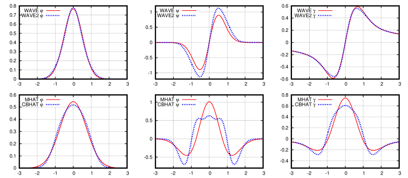
1. We use the wavelets called as CBHAT (“cowboy hat”) and WAVE2 that represent optimized modifications of the classic MHAT (“Mexican hat”) and WAVE wavelets. Just like WAVE and MHAT can be obtained by differentiating a Gaussian once or twice, the new optimal wavelets $\psi$ can be produced as derivatives of bell-like generating functions $\varphi$:

   $$\psi_{\rm WAVE2}(t)=\varphi_{\rm WAVE2}^{\prime}(t),\quad\psi_{\rm CBHAT}(t)=\varphi_{\rm CBHAT}^{\prime\prime}(t).$$ (1)

   Such wavelet transforms would highlight zones where the first or second derivative of the p.d.f. is large, revealing specific patterns like quick density gradients or p.d.f. convexities and concavities. The latters can be associated with clumps and gaps in the input sample.

2. The continuous wavelet transform (CWT) of the p.d.f. $f(x)$ is estimated from the random sample $\left\{x_{i}\right\}_{i=1}^{N}$:

   $$Y(a,b)=\int\limits_{-\infty}^{+\infty}\psi\left(\frac{x-b}{a}\right)f(x)dx$$

   $$\text{estimated by}\quad\widetilde{Y}(a,b)=\frac{1}{N}\sum_{i=1}^{N}\psi\left(\frac{x_{i}-b}{a}\right).$$ (2)

   Using similar formulae, the variance of $\widetilde{Y}$ is estimated too, in each point $(a,b)$.

3. With $\widetilde{Y}$ and its variance estimate, and also based on a comparison model $Y_{0}$ (possibly zero on start and updated iteratively), a normalized function $z(a,b)$ is constructed. This $z$ basically represents the Student $t$-statistic that have approximately constant noise properties over different $(a,b)$.

   A particular value $z(a,b)$, computed at any fixed position $(a,b)$, is asymptotically standard Gaussian, if $N\to\infty$. But this convergence is not uniform: for a particular finite $N$, even a large one, the quantity $z(a,b)$ won’t be Gaussian in some parts of the $(a,b)$ plane. For example, points with too small scale $a$ and points with $b$ far outside of the sample range must be removed from the analysis, as done by the next step.

4. Applying a criterion of Gaussianity on $z$, we determine the admissible work domain $\mathcal{D}$ in the $(a,b)$-plane. The simplest version of such a criterion is to have many enough sample objects $x_{i}$ that contribute in $\widetilde{Y}$ with a significant amount. This requirement can be formalized as:

   $$n(a,b)=\left.\sum_{i=1}^{N}\varphi\left(\frac{x_{i}-b}{a}\right)\right/\int\limits_{-\infty}^{+\infty}\varphi(t)dt\geq n_{\mathrm{min}}.$$ (3)

   The criterion guarantees that the distribution of $z(a,b)$ remains almost Gaussian and does not degenerate inside $\mathcal{D}$. However, more subtle Gaussianity criteria should be used in practice, and they are given in (Baluev, 2018).

   Larger samples imply larger $N$, causing $\mathcal{D}$ to expand to smaller scales $a$, while reducing $N$ causes $\mathcal{D}$ to shrink. Practical calculations revealed that for $N\lesssim 100$ the domain $\mathcal{D}$ becomes (almost) empty, so our pipeline is useful mainly for $N\gtrsim 100$.

5. Inside the work domain $\mathcal{D}$, we compute the maximum of $|z(a,b)|$. If this maximum is large enough, than there are significant deviations between the model $Y_{0}$ and the actual estimate $\widetilde{Y}$. The formal significance threshold can be estimated via the false alarm probability (FAP) using an analytic formula, which is based on the assumption that $z(a,b)$ is Gaussian:

   $${\text{FAP}}(z)\simeq 2W_{00}ze^{-z^{2}/2},$$ (4)

   where the coefficient $W_{00}$ can be determined simultaneously with the computation of $\widetilde{Y}$ and other quantities.

   Setting some small threshold ${\text{FAP}}_{*}$, e.g. $0.01$, and comparing the actual “observed” ${\text{FAP}}(z_{\rm max})$ with it, we can suppress the level of false detections to the desired low probability.

6. In practice, there are usually multiple places in the $(a,b)$ plane, where $|z(a,b)|$ rises above the significance threshold. Their location indicate the shift and scale characteristics of the structures that we need to add to $Y_{0}$ to obtain a more matching model. Peforming such a thresholiding, i.e. selecting $(a,b)$ points that satisfy ${\text{FAP}}(z(a,b))<{\text{FAP}}_{*}$, we purge the noise from the $(a,b)$ plane, and leave only significant structures.

7. After the noise thresholding, we can apply a generalized inversion formula

   $$f(x)=\frac{1}{C_{\psi\gamma}}\int\limits_{-\infty}^{+\infty}\int\limits_{-\infty}^{+\infty}Y(a,b)\gamma\left(\frac{x-b}{a}\right)\frac{dadb}{|a|^{3}},\\$$

   to the thresholded estimate $\widetilde{Y}(a,b)$. Here, the optimal kernel $\gamma$ depends on the adopted wavelet $\psi$, and they both define the normalization constant $C_{\psi\gamma}$. The inversion gives us an updated (or improved) comparison model $Y_{0}$ that includes all the significant structures detected at the current iteration.

8. The steps (3) and (5)-(7) are cycled over, until we remove all the significant structures from the $(a,b)$ plane (i.e., until $|z(a,b)|$ is suppressed below the significance threshold everywhere in $\mathcal{D}$). In the end we obtain a reconstructed p.d.f. estimate $\tilde{f}(x)$ that contains only details that overpassed the desired level of significance. In the process, we also obtain information about the FAPs for the particular details detected.

At a glance, the pipeline involves three big blocks algorithmically interleaved:

1. estimation of the wavelet transform and related stuff;

2. detecting significant structures;

3. iterative reconstruction of the p.d.f.

We note that the last one, the reconstruction of the p.d.f., represents a version of the matching pursuit method. From this point of view it becomes similar to the famous CLEAN (Roberts et al., 1987) and CLEANest (Foster, 1995, 1996) algorithms of the spectral deconvolution, which are also related to the matching pursuit (Hara et al., 2017).

Probably the closest wavelet analysis method in other works was provided by Skuljan et al. (1999). Let us list the main differences of our method from that one.

1. We avoid any binning of the data. The binning is an unnecessary and possibly intervening procedure in this task. The sample is analysed “as is”.

2. We consider more general formulations in many aspects: use of a general comparison model, of two distincts wavelets, and paying attention to both positive and negative values of the CWT. This enables us to detect a variety of distribution patterns. Skuljan et al. (1999) use zero comparison model, only the MHAT wavelet, and consider only positive deviations, limiting themselves to only the clumps detection.

3. Our analysis relies on a normalized statistic that allows to equibalance the noise over the shift-scale plane.

4. We corrected the significance testing approach to adequately treat the effect of the “domain penalty”. We compute the false alarm probability (FAP) based on the CWT extreme values within a work domain. Skuljan et al. (1999) assumed wrongly a single-value distribution, triggering hidden multiple comparisons and p-hacking in the final result. This effect is analogous to e.g. the well-known “bandwidth penalty” in the periodogram analysis (Schwarzenberg-Czerny, 1998; Baluev, 2008; Süveges, 2014), and it has a huge effect on the significance. Without taking it into account, the significance of a detection is dramatically overestimated, leading us to falsely confident conclusions.

5. The FAP is approximated in a completely analytic way, thus removing any need of Monte Carlo simulations to estimate the significance.

6. Our method utilizes an objective criterion to determine the useful work domain in the shift-scale plane.

7. We apply optimal wavelets that allow to improve the S/N ratio and to increase the admissible work domain. In particular, the MHAT wavelet is basically useless in this task, because of the large non-Gaussianity it generates (Baluev, 2018).

8. We built an optimized reconstruction kernel that allows to recover the p.d.f. from a “cleaned” CWT in a minimum-noise way.

9. The main limitation of our algorithm is that it can process only 1D distributions. It cannot analyse 2D distributions that were the main goal in (Skuljan et al., 1999), or distributions of higher dimension.

4 Demonstrative test applications

4.1 Pitfalls of the interpretation

As outlined above, our wavelets allows to detect distribution patterns of the following two types: (i) p.d.f. concavity/convexity, with CBHAT, and (ii) p.d.f. jump/fall, with WAVE2. The first type is related to the second derivative $f^{\prime\prime}(x)$, meaning that this pattern appears whenever $f(x)$ deviates from its local slope too much. The second type is related to $f^{\prime}(x)$, indicating the slope itself.

However, in practice it is usually impossible to imagine an isolated pattern of any of the above type. This implies certain difficulties with the interpretation of the analysis, so we need to consider some simulated teaching examples before we can proceed further.

In particular, it is necessary to acquire certain CWT “reading skills” before analysing any real-world data. For example, if the p.d.f. contains a narrow peak layed over some widespread background, it would imply the following patterns in the $(a,b)$-plane: (i) concavity in the left wing – central convexity – concavity in the right wing (with CBHAT), and (ii) a dipole-like uptrent–downtrend combination with WAVE2. A narrow transitional edge separating two statistically different families would look like just a single pattern with WAVE2 (say, an upturn), but with CBHAT it would imply a more complicated dipole-like sequence: left-wing concavity – (the upturn itself unseen with CBHAT) – right-wing convexity. Such illustrative examples are given in this section below.

The other difficulty comes from some deficiency of the p.d.f. reconstruction based on the matching pursuit. In the most basic words, the matching pursuit is aimed to seek a “sparse” (that is, a constructively compact) approximation to some raw data. It offers an easy and a quick solution, but not necessarily an accurate one. In particular, in the time-series analysis by CLEAN/CLEANest method there are difficulties with treating the aliases. A generally similar problem appears whenever wavelets mutually interfere in their side lobes (although it did not become that much important here).

In practice, the problem appears when e.g. two structures approach each other closely. In such a case, the reconstructed p.d.f. $f(x)$ may contain an artifact between them that does not reveal itself in the wavelet transform (in $z(a,b)$). Such an effect likely have common roots with the Gibbs phenomenon from the Fourier analysis.

Due to this effect, we currently consider the reconstructed $f(x)$ as just a useful hint that helps to intuitively interpret the 2D wavelet map. But if it comes to the significance estimate of any pattern, we must get back to $z(a,b)$.

4.2 Histograms and their uncertainties

The most basic and widely used tool of the distribution analysis is a histogram. We will use histograms as a demonstrative reference to compare with our wavelet analysis method. But first of all, we need to define some its formal characteristics and understand its statistical uncertainties.

Mathematically, the histogram is a sequence of empiric frequencies $\nu_{i}=n_{i}/N$, corresponding to $n_{i}$ objects falling inside an $i$th bin. An optimal bin size is given by the Freedman and Diaconis (1981) rule:

$$h=2\frac{\text{IQR}}{N^{\frac{1}{3}}},$$ (5)

where IQR is the interquantile range of the sample (counted from $0.25$ to $0.75$ quantile), and $N$ is sample size. However, in our cases this binning appeared insufficiantly fine, and loosing too much small-scale details, so we adopted a more dense grid. We actually set the total number of bins, $N_{\rm bin}$, rather than the bin width $h$, and we set $N_{\rm bin}=20$ everywhere below. This usually resulted in a roughly twice more dense binning than (5).

Since the distribution of each $n_{i}$ is binomial, the uncertainty of a given histogram box can be represented by the standard deviation

$$\sigma_{\nu_{i}}=\sqrt{\frac{p_{i}(1-p_{i})}{N}},$$ (6)

where $p_{i}$ is the actual (true) probability corresponding to the bin, $p_{i}=\int\limits_{{\rm bin}_{i}}f(x)dx$.

Since we need just a rough understanding of the histogram uncertaities, we will approximate the distribution of $\nu_{i}$ by the normal one (assuming that $n_{i}$ is large) and substitute the empiric $\nu_{i}$ in place of $p_{i}$ in (6).

The statistical deviation between some constructed model $\hat{f}(x)$ (hence model $\hat{p}_{i}$) and the empiric histogram $\nu_{i}$ can be expressed in terms of the normal quantiles $g_{i}=(\nu_{i}-\hat{p}_{i})/\sigma_{\nu_{i}}$. Furthermore, considering a single histogram bin, the normal quantile $g$ is tied to the false alarm probability, FAP, by the equations

$${\text{FAP}}=2\left[1-\Phi(g)\right],\quad g=\Phi^{-1}\left(1-\frac{{\text{FAP}}}{2}\right),$$ (7)

where $\Phi(x)$ is the cumulative distribution function of a standard normal variate. Thus, $g$ represents an absolute threshold such that a standard Gaussian random variable can exceed $\pm g$ only with probability FAP. The quantity $g$ is what is often understood under a “$g$-sigma” significance level.

However, this $g$ is useful only if we considered just a single histogram bin, selected prior to the analysis. It is illegal to rely on the usual $\sigma_{\nu}$ from (6), if the entire histogram consisting of $N_{\rm bin}$ bins is considered, which is a typical practical case. Statistically, different bins are almost independent from each other, and the probability to make a mistake on multiple bins is therefore larger than on a single bin. If we plainly set the FAP of each individual bin to the requred value, the probability to make a false alarm in the entire histogram would then scale up as

$${\text{FAP}}^{\prime}=1-(1-{\text{FAP}})^{N_{\rm bin}}\simeq N_{\rm bin}{\text{FAP}}$$ (8)

This is the effect of multiple testing that leads to an implicit degradation of any statistical accuracy. To compensate this effect, we should preventively set the FAP of an individual bin to a reduced value ${\text{FAP}}/N_{\rm bin}$. Then, taking into account (7), the corrected normal quantile would be

$$g^{\prime}(g)=\Phi^{-1}\left(1-\frac{1-\Phi(g)}{N_{\rm bin}}\right)$$ (9)

For example, for the one-sigma uncertainty, $g=1$ (hence ${\text{FAP}}=31.7\%$), we obtain the correction

$$g^{\prime}(1)=\Phi^{-1}\left(1-\frac{0.159}{N_{\rm bin}}\right)>1$$ (10)

Therefore, all the uncertainties (6) should be scaled up by multiplying them by $g^{\prime}$. For example, $N_{\rm bin}=20$ results in $g^{\prime}(1)=2.4$. Only such pumped uncertainties can be deemed as adequate $1$-sigma confidence intervals for the entire histogram.

To test the quality of the reconstructed p.d.f. models in an alternative manner, we also apply the Pearson chi-square goodness-of-fit statistic. It is defined as

$$X^{2}=N_{\rm bin}\sum_{i=1}^{N_{\rm bin}}\frac{(\nu_{i}-\hat{p}_{i})^{2}}{\hat{p}_{i}}.$$ (11)

Whenever our p.d.f. model is correct (all $\hat{p}_{i}=p_{i}$), the $X^{2}$ statistic approximately follows the $\chi^{2}$ distribution with $N_{\rm bin}-1$ degrees of freedom. In practice it is more convenient to approximate this $\chi^{2}$ distribution with the Gaussian one. For example, the following quantity is close to being Gaussian:

$$\sqrt[3]{\frac{X^{2}}{N_{\rm bin}-1}}\sim\text{Normal}\left(\mu=1-\frac{2}{9N_{\rm bin}},\sigma^{2}=\frac{2}{9N_{\rm bin}}\right).$$ (12)

Then, the standardized quantity

$$\tau=\left.\left[\sqrt[3]{\frac{X^{2}}{N_{\rm bin}-1}}-\left(1-\frac{2}{9N_{\rm bin}}\right)\right]\right/\sqrt{\frac{2}{9N_{\rm bin}}}$$ (13)

can be deemed as a direct analogue of the normal quantile $g$ from (7), though it corresponds to the entire histogram rather than to a single bin.

We use the Pearson test below mainly to demonstrate that our p.d.f. models agree with the sample, even though sometimes it might seem that they are oversmoothed. Large positive values of $\tau$ would indicate that our p.d.f. model (or $p_{i}$) disagrees with the sample. But all results presented below, either demonstative or real-world ones, will have large negative $\tau$. This indicates an expected overfit, i.e. that we intentionally seeked such p.d.f. model $\hat{f}(x)$ that approximates the sample well (even better than the true $f(x)$ would do). But regardless of this aggregated overfit, our analysis remains critical with respect to possibly noisy structural patterns, thanks to the strict significance threshold (4).

4.3 Graphical representation of the results

All figures that demonstarte results of our CWT analysis below, either of simulated or of real-world data, follow the same layout scheme. They contain $4$ graphs for each distribution analysed.

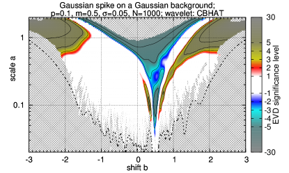
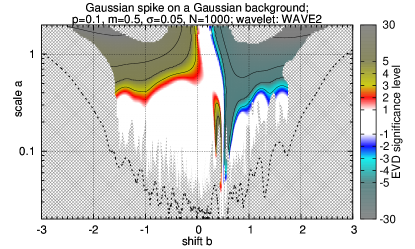
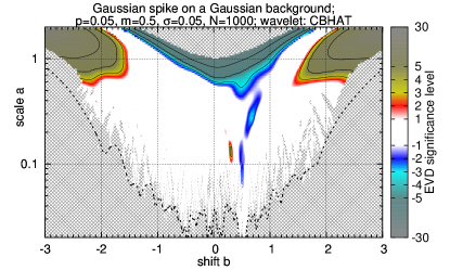
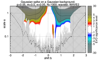
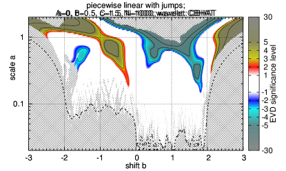
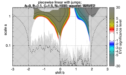
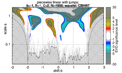
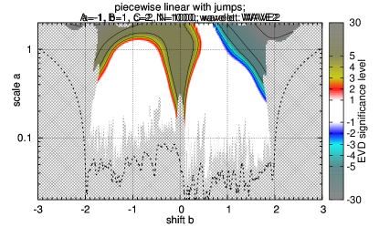
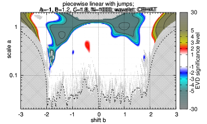
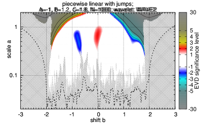
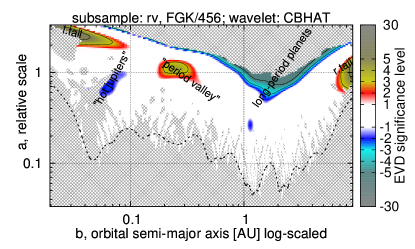
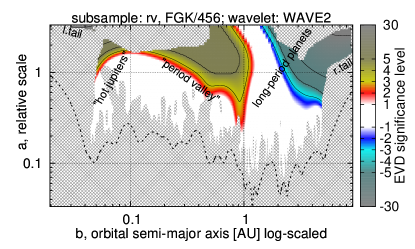
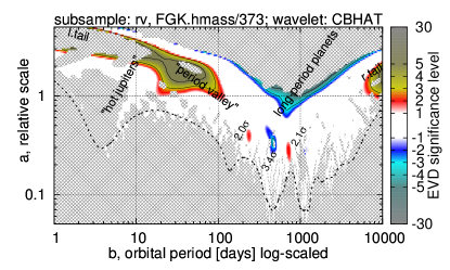
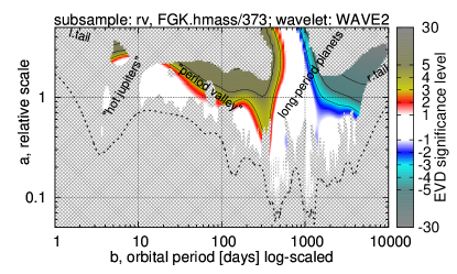
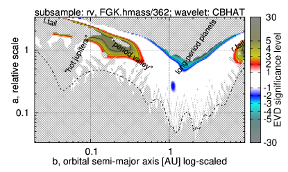
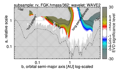
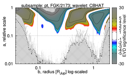
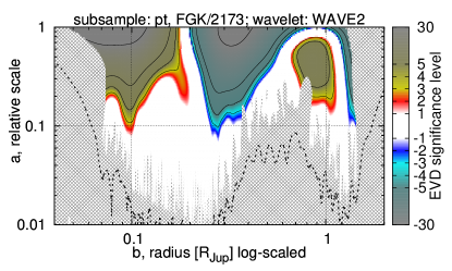
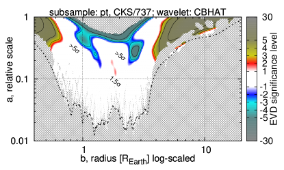
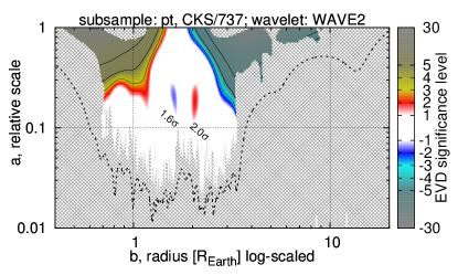
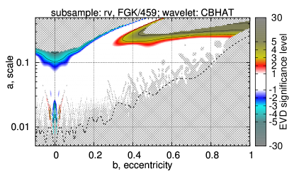
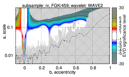
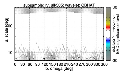
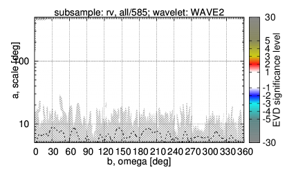
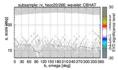
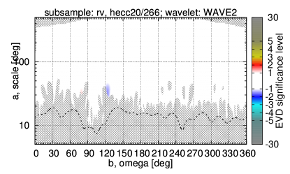
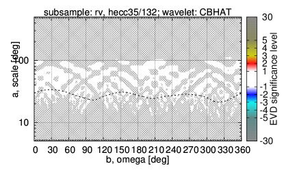
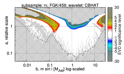
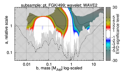
The top pair in each quadruplet represents the 2D significance colormaps for $z(a,b)$ for the CBHAT and WAVE2 wavelets. These colormaps are computed assuming the comparison model $Y_{0}=0$, i.e. they correspond to the starting iteration of the matching pursuit algorithm. Everything that appeared significant in these maps necessarily contributes to the corresponding reconstructed p.d.f.

The significance function is named as “EVD significance level” (with EVD standing for the Extreme Value Distribution). In absolute value, it equals to the Gaussian quantile $g$ from (7), where the FAP is calculated according to (4). Formally the function plotted in the 2D colormaps is $\pm g({\text{FAP}}(z(a,b)))$, where the sign is selected accordingly to the sign of $z$.

This significance is considered only inside the normality domain $\mathcal{D}$, and everything outside of $\mathcal{D}$ is hashed out. For the sake of an extra validation, we additionally plot the simplified normality criterion (3) as a dashed black curve. We note that generally this curve traces the lower boundary of $\mathcal{D}$ rather well, although important local deviations may appear.

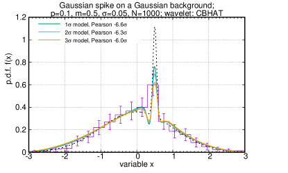
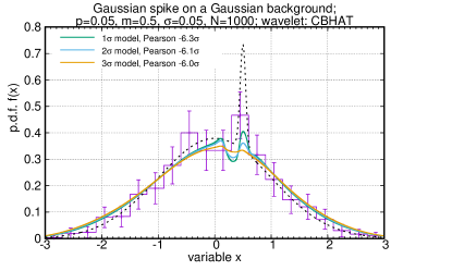
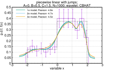
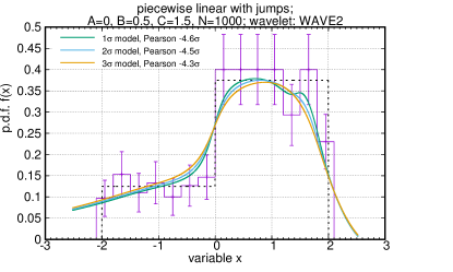
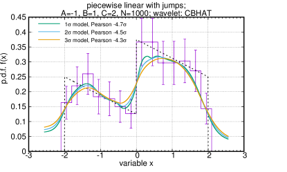
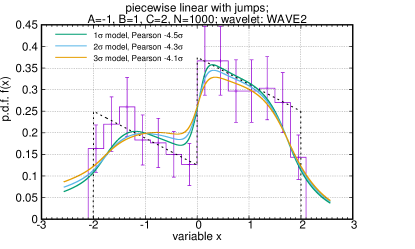
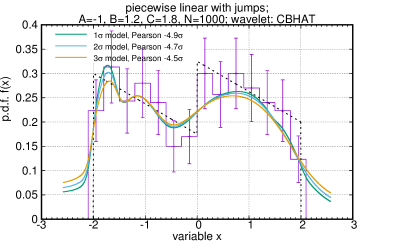
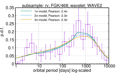
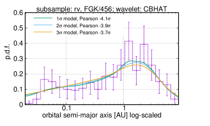
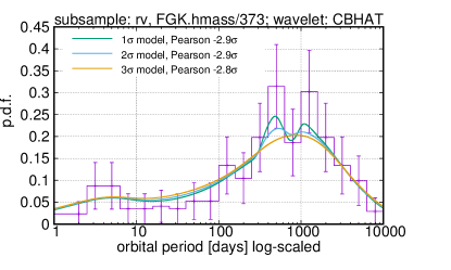
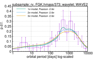
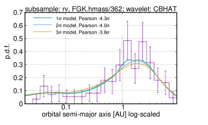
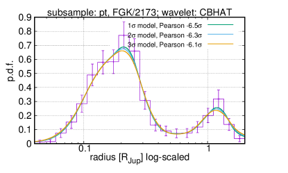
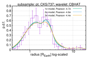
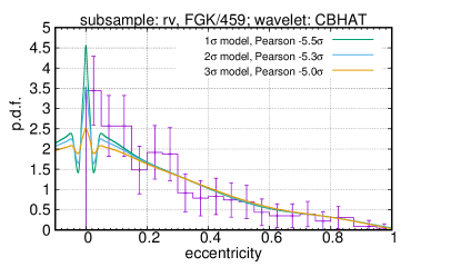
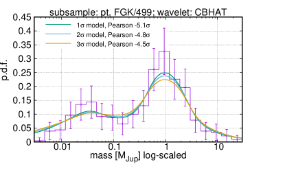
In the bottom pair of graphs of each quadruplet we show the corresponding histogram for $N_{\rm bin}=20$, along with the p.d.f. models obtained for three levels of noise tolerance, $g=1$ (green), $g=2$ (cyan), $g=3$ (yellow). The latter three curves differ only in color, because even in a grayscale plot it remains obvious, which one is which (larger smoothness means larger $g$).

It is necessary to draw attention to a couple additional details concerning the interpretation of the plots.

Whenever some pattern is detected in the 2D significance map and barely achieves e.g. $g=2$ at its maximum, this pattern has to be purged completely in the corresponding p.d.f. plot (for $g=2$). This might seem a bit paradoxical, but a two-sigma detail should normally disappear in a two-sigma p.d.f. model, though it should emerge, say, in the one-sigma curve in such a case. In general, to appear in a $g$-sigma model, the pattern must rise above this $g$ in the 2D significance map. Moreover, even if a structure does rise above the selected $g$-level, it still may appear practically invisible in the reconstructed p.d.f. model just because it is small in absolute magnitude (regardless of the high significance). Such a behaviour is normal and should not puzzle the reader.

4.4 Detecting a spike

We adopt the following double-Gaussian toy model:

$$f(x)=(1-p)\phi(x)+\frac{p}{\sigma}\phi\left(\frac{x-m}{\sigma}\right),\quad\phi(x)=\frac{e^{-\frac{x^{2}}{2}}}{\sqrt{2\pi}},$$ (14)

assuming that $\sigma$ is small.

We consider two cases: $p=0.1$ and $p=0.05$, with $m=0.5$ and $\sigma=0.05$ in the both.

Fig. 2 : Analysis of a simulated $N=1000$ sample: biased narrow Gaussian spike on a wide Gaussian background (14), with $p=10\%$, $\sigma=0.05$, $m=0.5$. Demonstrating significance maps of the wavelet transforms (top) and reconstructed p.d.f. curves for three levels of noise cleaning (bottom). The results obtained with the CBHAT and WAVE2 wavelets are shown in the left and right panels, respectively. In the bottom panels, the true p.d.f. is plotted by a dashed line, and the histogram of the sample is given, with the uncertainties computed via (6,9). A “standardized” Pearson test statistic $\tau$ from (13) for the synthesized p.d.f. models is also printed in bottom panels. See text for further details and discussion.

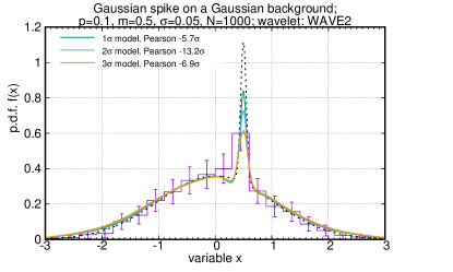The first case is shown in Fig. 2, and it demonstrates a robustly detectable spike well above the significance thresholds. The 2D CBHAT map reveal a specific small-scale pattern: a central p.d.f. convexity ($z<0$) accompanied by two smaller side concavities ($z>0$). This is a typical pattern that indicates an isolated subfamily: the concavities can be treated as separations between this family and the background.

It is very important that without detecting both those side concavities we cannot say for sure, whether the given structure is a statistically separated subfamily or it may represent something different. Or, saying it in other words, the decisive component of a subfamily is the p.d.f. concavities separating it from the rest of the sample, rather than the central concentration itself.

Fig. 3 : Simulated example: biased narrow Gaussian spike on a wide Gaussian background (14), as in Fig. 2 but with $p=5\%$, approximately corresponding to the detection limit.

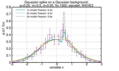For example, in Fig. 3 we present the analysis of a reduced $p=0.05$ spike that corresponds to a detection threshold. In this case the pattern in the CBHAT significance map is present only partially. We can see only the central convexity (rather clobbered due to the noise), and the clear left concavity. But the right concavity appeared insignificant because of the large noise. On the basis of only CBHAT analysis, we cannot say definitely, whether our pattern indicates: (i) a spike (concavity – convexity – unseen concavity), (ii) a gap (unseen convexity – concavity – convexity), (iii) an abrupt p.d.f. upturn (concavity – convexity), or even (iv) some more complicated wavy structure. The reconstructed p.d.f. models look like an inconclusive mixture of these interpretations.

The WAVE2 analysis may appear useful in such ambiguous cases, because it may provide highly complementary additional information. In the case of a spike substructire, the WAVE2 significance map reveals a diplole-like “upturn–downturn” structure. This enables an alternative interpretation of the subfamily boundaries. However, in the low-SNR case of Fig. 3 it appeared that the right slope of the spike still has only a moderate level of significance. Therefore, assuming a conservative detection threshold, our interpretation should remain inconclusive in this case.

To end this subsection, we note that histograms seem to be largerly useless in our task. Even in the high-SNR case (Fig. 2) their uncertainties appear too big for a robust detection of the spike. Morever, when looking for patterns like “spike” or “gap”, we must necessarily compare neighbouring histogram boxes. This becomes even more unreliable and less obvious, because the comparison of two or multiple noisy values (values with uncertainties) is a more intricate task than the comparison of a single noisy value with a model one.

We may notice that mutual comparison of different histogram boxes is what is roughly achieved with wavelets. According to Fig. 1, the CBHAT wavelet has such a shape that it averages some portion in a p.d.f. $f(x)$ and then subtracts the average side contributions. This is approximately the same as to subtract two side histogram bins from a middle one, within a triplet, and perform such an operation for multiple bin triplets (achieved by varying $b$) and for multiple histograms with different box width (achieved by varying $a$). However, wavelets allow to perform such a “brute force” search in a statistically safe way, taking into account the multiple testing penalty.

4.5 Detecting an abrupt upturn

Now we consider a piecewise-linear distributions $f(x)$, typically containing abrupt jumps:

$$f(x)=Ax+\left\{\begin{array}[]{ll}B,&x<0,\\ C,&x>0,\end{array}\right.\quad|x|\leq 2.$$ (15)

The abrupt jumps occur at the boundary points $x=\pm 2$ and at $x=0$. The linear slope $Ax$ was added to (15) to make the model more tunable.

Fig. 4 : Simulated example: piecewise linear distribution with jumps (15). Layout similar to Fig. 2. Notice a reconstruction artifact, appearing as a local drop in the p.d.f. at $x=1.3$, which is completely absent in the CWT significance map.

Fig. 5 : Simulated example: piecewise linear distribution with jumps (15). Layout similar to Figs. 2. Notice a Gibbs-like wavy artifact in the CBHAT p.d.f. reconstruction (left-bottom panel). These waves (in particular the concave minimum at $x=0.3$) are not present in the corresponding CWT significance map.

Fig. 6 : Simulated example: piecewise linear distribution with jumps (15). Layout similar to Figs. 2. Notice a Gibbs-like wavy artifacts in the p.d.f. plots, not confirmed by the CWT significance maps.

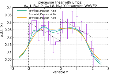With the WAVE2 wavelet, an abrupt upturn may appear just like a single pattern (spot) in the small-scale range of the $(a,b)$ plane. This behaviour is demonstrated in the top-right panel of Fig. 6. However, the small-scale spots may also merge with large-scale structures (if they have the same sign), so in practice it frequently looks as if the large-scale domain smoothly descended to smaller scales. This alternative behaviour is revealed in Figs. 4 and 5.

But we demonstrated above that upturns or downturns may also appear as parts of a gap or spike, rather than like a standalone structure. To separate such cases from each other, the CBHAT wavelet may be useful here. A “pure” upturn should ideally contain the following sequence: a starting concavity (seen with CBHAT), the upturn itself (seen with WAVE2), the final convexity (seen with CBHAT). This implies a dipole-like pattern in the CBHAT significance map, such that the WAVE2 structure is projected in its middle. Any more complicated configuration indicate hints of a more intricate structure than just a single upturn.

This is demonstrated in Fig. 4 and 5: the WAVE2 maps contain highly-significant structures near $b=0$, and they are accompanied by a CBHAT structures at $b=\pm 0.5$. Similar configurations are likely present at $b=\pm 2$, albeit they are less clear due to regions of non-Gaussianity.

These test examples also reveal that our p.d.f. reconstruction algorithm is affected by a Gibbs-like effect: abrupt jumps of high magnitude induce wavy artifacts. The matching pursuit algorithm assumes that the most “simple” p.d.f. model is simultaneously the most “economic” one in terms of the number of non-zero wavelet coefficients. But this most “economic” p.d.f. model is not always the least varying one. In some cases it might be necessary to include some statistically insignificant points from the $(a,b)$ plane, in order to obtain a more smooth p.d.f. reconstruction.

Summarizing this, we caution the reader against blind interpretation of the p.d.f. models presented below. They are offered as possibly helpful, but not decisive, interpretation of the wavelet significance maps. The p.d.f. artifacts do not affect the significance maps shown here. So, whenever it comes to the significance of a particular structure in $f(x)$, it is necessary to get back to the relevant 2D map that represents the main source of the significance information.

5 Constructing exoplanetary samples to be analysed

We utilize mainly the public database of the Extrasolar Planets Catalog (Schneider et al., 2011) available at www.exoplanet.eu. This database currently includes information and data about more than $3000$ exoplanets. However, this big ensemble appears too heterogeneous and needs to be split into several subsamples before performing any processing.

Since our analysis does not currently consider any formal treatment of the detection bias, we organize exoplanetary samples on the basis of their detection method. We construct two big subsamples: (i) planets detected by radial velocities, and (ii) planets detected by transits. These subsamples are not completely homogeneous yet, because they mix exoplanets discovered either in distinct Doppler or distinct transit surveys that differ in their accuracy and time base. This implies some differences in the corresponding “detection windows” that overlap with each other in a complicated way. We should bear this in mind, although it is unlikely that such a mixing effect would distort small-scale distribution details.

Our method can currently handle only unidimensional distributions, and this implies further complications. There are multiple parameters associated to an exoplanet, and different parameters reveal correlations forming complicatedly shaped structures in the multidimensional space. Considering just single-dimensional distributions would mean to look at 1D projections of these structures. This infers information losses, in particular a decrease in sharpness. To suppress this effect to a certain degree at least, we can deal with various slices of the parametric space. We construct them by cutting the full exoplanetary sample with respect to some crucial parameters. These ‘cut parameters’ are different from the ‘target parameter’ that defines what distribution is investigated.

Simultaneously, we should take care about the sizes of the resulting samples when manipulating with them. In practice it appeared that samples smaller than $100$ objects are useless in the analysis, because entire or almost entire shift-scale plane becomes non-Gaussian. Moreover, at least $300$ objects are needed to obtain some informative non-trivial results.

Our main samples that we used in the analysis, are listed in Table 1. Note that some values were missed for some planets in the database, so when considering the distribution of particular parameters, the actual sample size can appear smaller than shown in the table.

Table 1 : Basic exoplanetary samples used in the work.

sample id	$N$	description
rv	$708$	Planets detected by radial velocity
rv.FGK	$468$	As above, but FGK stars only ($M_{\star}\in[0.6,1.4]M_{\odot}$)
rv.FGK.hmass	$373$	As above, but only giant planets ($m\sin i\geq 0.3M_{\mathrm{Jup}}$)
pt	$2730$	Planets detected by primary transit
pt.FGK	$2193$	As above, but FGK stars only ($M_{\star}\in[0.6,1.4]M_{\odot}$)
pt.CKS	$737$	California Kepler Survey sample cleaned similarly to (Fulton et al., 2017), see Sect. 6.2.

We did not limit ourself to just drawing data from The Extrasolar Planets Encyclopaedia. Additionally we tried to reproduce the California Kepler Survey (CKS) sample that was used by Fulton et al. (2017) in their analysis of exoplanetary radii distribution. Using the data from (Petigura et al., 2017; Johnson et al., 2017), we followed the same steps: removed known false positives, removed stars with $K_{p}>14.2$, put the constraints on the orbital period $P<100$ d and on the impact parameter $b<0.7$, removed giant stars using the same criterion as in (Fulton et al., 2017), and limited the temperature range by $4700-6500$ K.

Unfortunately, we failed to reproduce the final sample precisely. The most problematic stage was filtering $b<0.7$. The cited works lack the values for $b$ and do not mention were they taken from, so we decided to extract $b$ from the NASA Exoplanet Archive. It appeared, however, that the final sample shrinked to $N\sim 700$, which is smaller than $N\sim 900$ in Fulton et al. (2017). We therefore decided that these values of $b$ from the NASA archive might be less trustable, and then softened the threshold a bit, $b<0.8$. But to compensate for an increased fraction of possibly unreliable radii estimates, we added an extra constraint that the relative uncertainty in the planet radius must be below $0.1$. Thus we had $N=737$ planet candidates left in the sample.

6 Results of the analysis

6.1 Orbital periods and semimajor axes: fine-structured iceline accumulation?

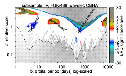
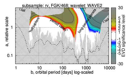
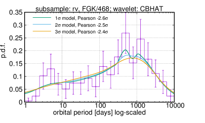
Results for the period and semimajor axis distributions (both in logarithmic scale) are shown in Fig. 7 and 8. They refer to the rv.FGK subsample. It is well-known that these distributions should behave similarly, thanks to the third Kepler law, so we consider them here together.

Fig. 7 : Wavelet analyis of known exoplanetary candidates. Subsample: RV detection method, FGK-type host stars, $N=468$. Variable: orbital period. The figure layout is the same as in Fig. 2.

Fig. 8 : Wavelet analyis of known exoplanetary candidates. Subsample: RV detection method, FGK-type host stars, $N=456$. Variable: orbital semimajor axis. The figure layout is the same as in Fig. 2.

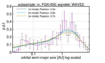First of all, we can see the large-scale structure: a highly-populated wide peak of long-period “warm jupiters”, a shallow concentration of “hot jupiters” at short periods, and a wide “period valley” between them. These are well-known features, more or less succesfully explained by contemporary simulation works on planet formation and migration, see e.g. Ida and Lin (2004, 2008) and many more.

In particular, the predominant WJ maximum is attributed to the effect of the so-called iceline accumulation. It was explained in (Ida and Lin, 2008) and extensively studied in many works after (e.g. Schlaufman et al., 2009; Hasegawa and Pudritz, 2013). Near the snow line physical processes of ice particles migration, evaporation, outward diffusion and recondensation interact so that the density of the material increases. This favours to planet formation just beyond the ice line. Moreover, if a protoplanet grows to form a giant planet (above Saturn or Jupiter mass), it then migrates modestly, so that the corresponding concentration of giant planets gets shifted inward.

The inner boundary of the WJ family corresponds to the semimajor axis $A\sim 1$ AU or orbital period $P\sim 300$ d.

In Fig. 7-8 we can also see a fine-structured pattern, in the period distribution especially. It appears as a smaller-scale local maximum layed over the large-scale one, close to the upper boundary of the PV depression. In the reconstructed p.d.f. curves this substructure looks like an overshoot peak, maybe even causing a bimodality. However, we must be careful with these curves due to possible artifacts of the matching pursuit. To gain more accurate understanding of what actually happens there, we must refer to the corresponding wavelet transforms.

Let us focus on the period distribution at first, Fig. 7.

In its CBHAT wavelet transform, we can see a remarkable negative (cyan) spot at $P\sim 450$ d, with a relatively small scale $a\sim 0.3$. It reaches $3$-sigma level that confirms its high significance. Such a spot indicates that the p.d.f. attains a high curvature at this location (with upward convexity). This does not necessarily indicate a local maximum, but at least a zone of relatively abrupt transition between the PV and WJ domains.

Such an abrupt transition is confirmed by the WAVE2 transform, where we can see a high-significe domain near $P\sim 350$ d that descends to the same small scales.

All this suggests the following interpretation concerning the $\log P$ distribution of the rv.FGK sample:

1. there is a quick density gradient near $P\sim 350$ d, corresponding to the PV/WJ boundary;

2. this gradient ends with a highly-curved p.d.f. convexity near $P\sim 450$ d that further turns into the wide maximum of long-period planets.

At this stage we still cannot say, if there is indeed an additional local maximum at $P\sim 450$ d or any separated subfamily of exoplanets.

To ensure that we talk about a subfamily, we would need to detect some side separations from the remaining sample of planets. That is, the small-scale spot at $P\sim 450$ d in the CBHAT wavelet map should be accompanied by a couple of counter-signed spots on both sides. They would indicate concave zones in the p.d.f., meaning that the central convexity represents a standalone formation.

In fact, we do note some secondary spot in Fig. 7, but unfortunately its significance is too small, below $g=2$.

Now we can use theoretic results to decide what sample to analyse further. Simulations of the iceline barrier effect from e.g. (Ida and Lin, 2008) predict that in the range of interest, $P\sim 300-1000$ d, less massive planets would only represent an interfering background that blurs the giant planets subsample. The positions for the “Warm Jupiters” and “Warm Neptunes” maxima should be displaced considerably, because their migration histories are different. Therefore, it might be reasonable to analyse the subsample of giant planets, rv.FGK.hmass. This subsample should reveal the iceline accumulation effect in a more clean manner.

Fig. 9 : Wavelet analyis of known exoplanetary candidates. Subsample: RV detection method, FGK-type host stars, higher-mass planets ($m\sin i>0.3M_{\rm Jup}$), $N=373$. Variable: orbital period. Fine-scale structures are labelled with the significance quantile $g$. The figure layout is the same as in Fig. 2.

Fig. 10 : Wavelet analyis of known exoplanetary candidates. Subsample: RV detection method, FGK-type host stars, higher-mass planets ($m\sin i>0.3M_{\rm Jup}$), $N=362$. Variable: semimajor axis. The figure layout is the same as in Fig. 2.

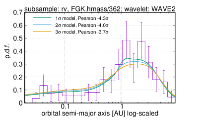These results are presented in Fig. 9-10. We can see that all the fine-scale structures within the range $P\sim 300-1000$ d indeed gained more magnitude. In the CBHAT wavelet transform, we can see the primary (negative) spot at $P\sim 450$ d that got the significance $g=3.4$, accompanied by a pair of the counter-signed secondary spots at $P\sim 700$ with $g=2.1$, and at $P\sim 250$ d with $g=2.0$. Such a triplet pattern highlights a statistically separated narrow subfamily of giant planets in the period range $\sim 300-600$ d. In the p.d.f. graph it looks like an overshooting peak right after an upturn.

This significance increase was achieved by restricting the exoplanetary sample from rv.FGK to rv.FGK.hmass, but this is not a p-hacking or data-dependent analysis. It would be those, if we just searched many subsamples in the hope to finally obtain a desired significant result. But our decision of how to restrict the sample relied on the previous theoretic knowledge, regardless of any statistical analysis already done. The second sample could equally decrease the significance of the result rather than increase it. In such a case, this subsequent analysis attempt does provide additional evidence.

In either case, there is no significant hints of bimodality within the WJ maximum. Although some of the p.d.f. plots, e.g. in Fig. 9, suggest bimodality, it looks like a reconstruction artifact appearing due to inherent weaknesses of the matching pursuit algorithm.

So far we considered only the period distribution, but orbital semimajor axes are apparently more appropriate concerning the iceline barrier effect. Disappointedly, this distribution does not reveal so much subtle details (Fig. 8,10). With the CBHAT wavelet, we can see just a single small-scale spot at $A\sim 1.1$ AU indicating a local convexity. In the subsample of giant exoplanets, its significance barely reaches the two-sigma level, and it becomes even worse in the larger rv.FGK sample.

The semimajor axis $A$ is merely a derived parameter, while the primary “observed” quantity is the orbital period $P$. Knowing $P$, we can recover $A$ using the third Kepler law:

$$P\propto M_{\star}^{-\frac{1}{2}}A^{\frac{3}{2}},\quad A\propto M_{\star}^{\frac{1}{3}}P^{\frac{2}{3}},$$ (16)

where $M_{\star}$ is the star mass. However, the value of $M_{\star}$ is not the same for all exoplanets. In this case (16) defines a statistical correlation between $P$ and $A$ rather than a strict binding. That is, the $P$- and $A$-distributions should look generally similar, but small-scale details would be different due to the scatter in $M_{\star}$. If a detail appeared sharp in the $P$-distribution, it gets blurred in the $A$-distribution, and vice versa. It cannot remain sharp in the both.

Our analysis revealed that small-scale subfamily discussed above appears sharply in $P$. But then it should necessarily fade out in $A$. Since this is a necessary and predictable behavior, it does not make the detection less reliable from the statistical point of view.

But then an interesting question emerges: should the iceline barrier effect generate more sharp details in $a$- or $P$-distribution? Unfortunately, simple considerations did not provide us with a definite answer. By combining (16) with the inverse-squares law, it is easy to assess the distance of the ice line, $a_{\mathrm{ice}}$, and the corresponding Keplerian period, $P_{\mathrm{ice}}$, as a function of the star luminosity:

$$L_{\star}A_{\mathrm{ice}}^{-2}=\mathop{\text{const}}\nolimits\implies\quad A_{\mathrm{ice}}\propto L_{\star}^{\frac{1}{2}},\quad P_{\mathrm{ice}}\propto M_{\star}^{-\frac{1}{2}}L_{\star}^{\frac{3}{4}}.$$ (17)

And by applying the mass-luminosity relation, $L_{\star}\sim M_{\star}^{4}$, we obtain

$$A_{\mathrm{ice}}\sim M_{\star}^{2},\qquad P_{\mathrm{ice}}\sim M_{\star}^{-\frac{5}{2}}.$$ (18)

But then it follows that both the $A$- and $P$-distributions should be blurred approximately equally, because $A_{\mathrm{ice}}$ and $P_{\mathrm{ice}}$ depend on $M_{\star}$ via almost the same power degree ($2$ or $-2.5$, the sign does not matter).

However, the formulae (18) do not take into account the migration of planets. The migration rate and its distance should correlate with $M_{\star}$ somehow, but this correlation depends on multiple factors. It is difficult to predict without performing simulations like those available in (Ida and Lin, 2008). Depending on the sign of the correlation, it may sharpen either of the two distributions. In principle, this can be used to verify the iceline nature of the exoplanetary subfamily for $P\sim 300-600$ d.

At last, we recall that the database of The Extrasolar Planets Encyclopaedia is heterogeneous, mixing planet candidates discovered by multiple independent Doppler programmes. Such mixed samples might demonstrate spurous effects due to an overlap of different detection thresholds. However, most radial-velocity surveys are very aged already, and they are pretty complete in the period range of $300-600$ d (for giant planets at least). Moreover, the orbital period $P$ is one of the best-determined exoplanetary characteristics. It is therefore unlikely that observational selection, sample heterogenity, or possibly inaccurate data could cause any unusual statistics in this period range.

6.2 Transiting planets radii: confirming evaporation valley

The radii distribution among Kepler exoplanetary candidates demonstrates signs of a bimodality (Fulton et al., 2017). There are two local maxima of the density at $R=1.3R_{\oplus}$ and $R=2.4R_{\oplus}$, while planets with $R$ in the intermediate range $1.5-2.0R_{\oplus}$ are comparatively rare. This effect was named the “evaporation valley”, and it has got a detailed theoretic treatment already (Owen and Wu, 2017). In a few words, higher-mass planets are capable to preserve their dense atmospheres even if they are exposed to intense irradiation from the star, but low-mass planets loose most of their atmospheres eventually, reducing their sizes to even smaller values than they initially were.

Fig. 11 : Wavelet analyis of known exoplanetary candidates. Subsample: Primary transit detection method, FGK-type host stars, $N=2173$. Variable: planet radius. The figure layout is the same as in Fig. 2.

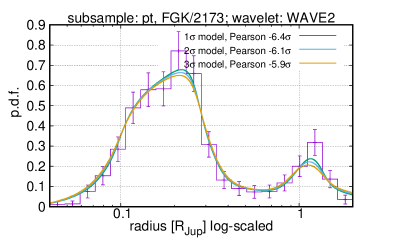We were interested to apply our algorithm to this case. First of all, we followed our common protocol set in advance, i.e. we analysed the transit sample pt.FGK, drawn from the database of The Extrasolar Planets Encyclopaedia. This sample includes Kepler candidates, as well as those detected by more common but less sensitive ground-based surveys. The results for the planet radii distribution are shown in Fig. 11.

A bimodality is obvious in the reconstructed p.d.f., though this is unrelated to the “evaporation valley”. The peaks are for the families of giant Jupiter-sized planets and of the Earth-/superearth-sized ones. They are separated by a wide minimum in the range $0.4-0.8R_{\mathrm{Jup}}$. These major families with an intermediate desert are undoubtful, and were predicted quite early, at least by Ida and Lin (2004).

Apparently nothing related to the “evaporation valley” can be spotted in this p.d.f., but we can see in the CBHAT wavelet transform a small negative (blue) spot located at $R\sim 0.12R_{\mathrm{Jup}}$ or $1.3R_{\oplus}$. It represents a hint of a smaller-scale p.d.f. convexity. Its significance is above two-sigma, but the absolute magnitude appears so small that practically nothing can be seen in the reconstructed p.d.f., or even in the histogram, at this location.

In the WAVE2 wavelet transform there is a fancy anomaly at $R=0.2R_{\mathrm{Jup}}$ and $a=0.2-0.3$, indicating a relatively more quick p.d.f. upturn at this location, though it is not obvious in the reconstructed model.

Likely, these subtle hints is all what is left from the “evaporation valley” in this sample. The database in (Roques and Schneider, 1995) is extremely heterogeneous for transiting planets. And contrary to the previous subsection, we are now interested in the range where many surveys appear incomplete. Transit programmes have different detection limits, and their selection functions get overlayed, imposing spurous distortions to the statistics. Besides, it seems that this catalog is quite “dirty” with respect to false positives and unreliable values. It is not very much surprising that the “evaporation valley” could not be reliably reproduced with these data, although our method was able to detect some remaining hints.

Fig. 12 : Wavelet analyis of known exoplanetary candidates. Subsample: California Kepler Sample (CKS) with filters (see text), $N=737$. Variable: planet radius. Fine-scale structures are labelled with the significance quantile $g$. The figure layout is the same as in Fig. 2.

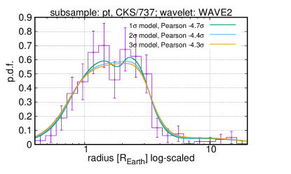After that, we applied our analysis to the more homogeneous CKS data cleaned as described in Sect. 5. The results are shown in Fig. 12. Now we can clearly see a bimodal radii distribution with maxima at $1.3R_{\oplus}$ and $2.6R_{\oplus}$, and a gap between. Though our sample is not strictly the same as in (Fulton et al., 2017), the histogram does not reveal any obvious visual difference.

But contrary to Fulton et al. (2017), our analysis does not provide so strong statistical support to the bimodality. Although the CBHAT wavelet clearly reveals a pair of convexity zones at $1.3$ and $2.4R_{\oplus}$, the concavity between them does not reach enough significance. The convexities are undoubtful, but on themselves they do not yet tell anything in support of the bimodality and do not confirm standalone exoplanetary families. Without a clear intermediate gap, the density function may have just a plateau-like shape with more abrupt sides. That would mean just a single density maximum without any submafilies.

Ensuring the bimodality necessarily requires to detect a gap, or at least an intermediate concavity. However, this feature does not appear statistically significant with the CBHAT wavelet (only $g=1.5$). A concavity and even a local minimum is obvious in the reconstructed p.d.f. even for $g=3$, but this looks like an artifact of the matching pursuit algorithm, since such a significance level is not supported by the wavelet transform. So, the CBHAT wavelet fails to detect the “evaporation valley”.

The WAVE2 transform in Fig. 12 appears a bit more promising: it resolves a dipole-like standalone pair of downturn/upturn patterns, and the upturn part at $R=2R_{\oplus}$ appears moderately significant, $g=2$.

Being puzzled by such an inconsistency with Fulton et al. (2017), we investigated the argumentation from that work.

1. Non-parametric Kolmogorov–Smirnov and Anderson–Darling tests to verify the agreement with a loguniform distribution. Even if the $R$-distribution does deviate from the loguniform one significantly, this conclusion tells us nothing in favour of possible bimodality. There are many unimodal distributions that could be different from the loguniform one. The K–S and A–D tests are incapable to provide any information concerning multimodality. They are not decisive in this task.

   Besides, the application of those tests seems illegal, because the loguniform model was not completely specified a priori. The left and right cutoff positions were unknown to the authors a priori and were guessed from the same data, which is a condition for data-dependent analysis.

2. The dip test of unimodality by Hartigan and Hartigan (1985). The test is well-known and useful in itself, but its application nonetheless seems invalid due to a hidden pre-analysis. It is likely that the authors decided to apply this particular very specific test only because the bimodality was initially suspected by visual inspection of the histogram for the same Kepler data. If the data were different then such a suspection would not appear, and the question of bimodality would not arose at all. In such a case, some other pecularity could be spotted, triggering the use of another specific test designed to detect patterns of that type. Again, we can clearly see a condition for a data-dependent analysis: the hypothesis was formulated from the same data that were then tested as if this hypothesis was given in advance.

   We nonetheless applied the Hartigan and Hartigan (1985) test to our version of the CKS sample to compare the results. We failed to reproduce the same high significance level as Fulton et al. (2017). Instead of ${\text{FAP}}=0.14$ per cent (or $g=3.2$), for the $\log R$ data we obtained merely ${\text{FAP}}=3$ per cent or $2.2$-sigma significance. If it is not a software bug in either work then the test itself might be not very robust. We considered other CKS subsamples, filtering the data at different levels of tolerance. The best significance from the dip test was ${\text{FAP}}=0.6$ per cent, if we preserved the radii with uncertainties greater than $10$ per cent. However, even this significance is much worse than Fulton et al. (2017) reported.

3. Fitting a spline model and spline deconvolution. The main conclusion was that because of a $\sim 12$ per cent uncertainty in the planet radii, the “observed” $R$-distribution is merely a smoothed version of the original, “underlying”, distribution of the precise radii. Hence, the true distribution must have a deeper bimodality gap than it seems from the observation.

   There is no doubts on this conclusion, but it does not offer us any additional evidence in favour of the bimodality, because it has nothing to do with the statistical significance. The true gap should be deeper only if it actually exists, i.e. if the observed one is not a noise artifact. Otherwise, the gap just does not exist in the both distributions.

The conclusion is that the hints of the gap in the radii distribution are not ignorable, but its significance remains rather marginal. Its reliability is much worse than Fulton et al. (2017) claimed. We definitely cannot give it any “strong support”. An optimistic significance estimate is about two-sigma level.

6.3 Orbital eccentricities

We treated the orbital eccentricity $e$ as a symmetric parameter, extending its distribution to the negative range, $e\Leftrightarrow-e$. This was necessary to avoid an artificial distribution cutoff at $e=0$, in order to process the low-eccentricity domain more adequately. To reach this goal, we duplicated every $e$ value in the sample with $-e$. Thus we artificially increased the sample size to $2N$, but when computing the significance and related stuff, we substituted the correct size of just $N$, so that such a manipulation should not lead to an overestimated significance. Also, we consider our work domain $\mathcal{D}$ only for $e\geq 0$, so the coefficients in the FAP estimate (4) do not get doubled (this would lead to an underestimated significance otherwise).

We recognize that even with such corrections the analysis might be not fully rigorous, because instead of the pure CBHAT and WAVE2 we basically use wavelets of a different shape, symmetrized about zero. The actual remaining effect is not obvious, but we did not try to treat it better, because we did not obtain any remarkable results with this distribution.

Fig. 13 : Wavelet analyis of known exoplanetary candidates. Subsample: RV detection method, FGK-type host stars, $N=459$. Variable: orbital eccentricity. The figure layout is the same as in Fig. 2.

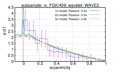The results for the rv.FGK sample are presented in Fig. 13. We can see an intricate small-scale structure near $e=0$ that consists of a very narrow peak accompanied by narrow side gaps. Such a structure near $e=0$ is not surprising and it can be explained by the following obvious sources:

1. Deficient RV data are usually fitted with the eccentricity fixed at zero. This leads to an increased height of the $e=0$ peak, because some exoplanets with non-zero $e$ are reset to zero.

2. If the eccentricity is fitted, it is frequently biased to a larger value due to a non-linearity in the Keplerian RV model. This bias moves some exoplanets with small $e$ away from zero, forming a gap about $e=0$ that serves as a background for the central very narrow peak.

3. There is a well-known physical phenomenon of tidal circularization that settles many “hot jupiters” to $e\approx 0$, further increasing the central peak.

We can see that only the third effect is physical and related to the actual eccentricity distribution, while the other two are only apparent effects imposted by the RV data fitting.

We did not reveal any other small-scale structures in this distribution. Also, we did not analyse transit candidates here, since most of them do not have a good eccentricity estimate.

6.4 Orbital periastra: no hints of a detection bias

We analysed the distribution of the orbital pericenter argument, $\omega$. Our motivation was to detect possible selection effects. Any detection bias in $e$ should reveal itself in the $\omega$ too, because the shape of the eccentric Keplerian RV curve depends on $\omega$ dramatically. In the eccentricities we cannot disentangle this bias from the actual distribution shape, which is unknown. However, the spatial orientation of exoplanetary orbital periastra should likely be isotropic, meaning a uniform distribution in $\omega$. Therefore, any deviation from the uniform distribution would immediately indicate a detection bias.

Fig. 14 : Wavelet analyis of known exoplanetary candidates. Subsample: RV detection method, cutting higher eccentricities ($e>0.15$, $e>0.20$, $e>0.35$). Variable: argument of the periastron. The figure layout is the same as in Fig. 2.

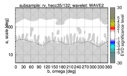The results for the $\omega$-distribution (the rv sample) are presented in Fig. 14. Additionally to this full sample, we also computed wavelet maps for various subsamples by removing low-eccentric exoplanets ($e<0.15,0.20,0.35$). In either case, the distribution is consistent with the uniform one. No significant deviation was detected.

Note that to avoid non-physical cutoffs at $\omega=0$ and $\omega=2\pi$, we applied an approach similar to that from Sect. 6.3: we replaced every sample value $\omega$ with a triplet $\omega-2\pi,\omega,\omega+2\pi$. This artificially increased the total sample size to $3N$, but we again used just $N$ in the significance estimates where appropriate.

6.5 Planet masses

Finally, we present our results for the exoplanetary mass distribution. In this analysis, we considered the rv.FGK and pt.FGK samples. Note that the second (transit) sample appeared much smaller than e.g. transit sample in Sect. 6.2, because the planet mass can be determined only by radial velocities. Most transiting planet candidates remain unconfirmed by the Doppler method, mainly because of technical limitations on faint stars. As a result, both the samples appeared to have almost the same moderate size, $N\sim 500$.

Fig. 15 : Wavelet analyis of known exoplanetary candidates. Subsample: RV detection method, FGK-type host stars, $N=459$. Variable: planet minimum mass $m\sin i$. The figure layout is the same as in Fig. 2.

Fig. 16 : Wavelet analyis of known exoplanetary candidates. Subsample: Primary transit detection method, FGK-type host stars, $N=499$. Variable: planet mass $m$. The figure layout is the same as in Fig. 2.

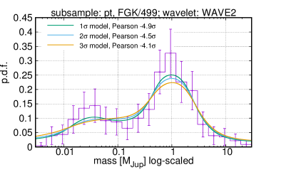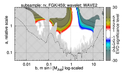
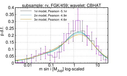
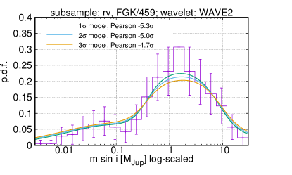
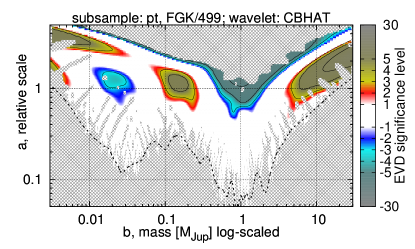
The results are presented in Fig. 15 (rv.FGK sample, distribution of $m\sin i$) and in Fig. 16 (pt.FGK sample, distribution of $m$). In the first case, the distribution appears unimodal with a wide maximum covering the range $m\sin i=0.5-5M_{\rm Jup}$. On contrary, the transit sample reveals an undoubtful bimodality, with a secondary maximum at $m\sim 0.03M_{\rm Jup}$ (or $\sim 10M_{\oplus}$). The first maximum involves giant exoplanets, while the second one incorporates super-earths and Neptune-mass planets. The gap between the families covers the range $m=0.1-0.3M_{\rm Jup}$.

We may conclude that the transit detection technique is remarkably more sensitive to low-mass planets. Although all exoplanets in the both samples were observed by the radial velocity technique, the transit candidates required just an independent follow-up Doppler confirmation, which is much easier than to make a detection.

We did not detect any small-scale details in the exoplanetary mass distribution.

7 Some self-crititicism concerning the significance estimates

Unfortunately, the issue of a hidden p-hacking effect often appears very difficult to overcome completely. The numeric significance levels reported above are still not entirely free from an overestimation caused by multiple testing.

First of all, we always considered two wavelet transforms simultaneously, WAVE2 and CBHAT. Hence, our analysis hiddenly involved two comparison tests, on the same distribution. The number of false alarms should then appear larger than expected from just a single wavelet transform. In fact, our test involved the maximum between two distinct test statistics, namely $\max(z_{\rm WAVE2},z_{\rm CBHAT})$, rather than the maximum of just a single $z(a,b)$.

Assuming that the maxima on the WAVE2 and CBHAT wavelet maps are uncorrelated with each other, we should roughly double the FAP estimate. This implies the need of a multiple testing correction, analogous to (9) with $N_{\rm bin}=2$:

$$g^{\prime}=\Phi^{-1}\left(\frac{1+\Phi(g)}{2}\right),\quad g=\Phi^{-1}\left[2\Phi(g^{\prime})-1\right].$$ (19)

Now, $g^{\prime}$ is the value actually obtained from the significance map (assuming no multiple testing), and $g$ is the corrected significance taking into account the double testing penalty.

For the subfamily $P=300-600$ d we obtained in Sect. 6.1 the following detection significances in our CBHAT analysis: $g=2.0$ (left concavity), $g=3.4$ (central convexity), and $g=2.1$ (right concavity). Formula (19) transforms these levels to the following: $g^{\prime}=1.6$, $g^{\prime}=3.2$, and $g^{\prime}=1.8$. The central convexity still remains pretty convincing, but the side separations appear to have just a marginal significance.

For the CKS radii distribution we obtain with CBHAT: $g>5$ (left maximum), $g=1.5$ (central gap), $g>5$ (right maximum), and with WAVE2: $g=1.6$ (descent to the gap) and $g=2.0$ (ascent out of the gap). Using (19), this is corrected to: $g^{\prime}>5$ (left maximum), $g^{\prime}=1.1$ (central gap), $g^{\prime}>5$ (right maximum), $g^{\prime}=1.2$ (descent to the gap) and $g^{\prime}=1.6$ (ascent out of the gap). We can see that the gap becomes insignificant.

But from the other side, the WAVE2 and CBHAT wavelet maps should be correlated: if a pattern is detected by one of the wavelets, the other wavelet should likely reveal something unusual too. Therefore, the correction (19) is probably too conservative. Moreover, our FAP estimate (4) was made conservative by design, because should tend to overestimate the actual FAP. It might seem likely that these effects could in turn compensate each other, so the uncorrected $g$-levels might be more realistic than $g^{\prime}$ from (19).

But more difficulties appear because we actually need the significance of combined patterns that involve several elementary structures on the wavelet maps. For example, to ensure that the subfamily $P=300-600$ d does exist, we needed the whole triplet “concavity-convexity-concavity” to be confirmed as a whole. Just a single central convexity without side concavities is notable, but we would not classify it as a “subfamily”, because a subfamily should be separated in some way from the background planets. Without a separation, it should be interpreted just as relatively abrupt PV/WJ transition, but not as a separate family.

Similarly, when detecting the bimodality in the radii distribution, we needed to ensure the significance of the triplet “convexity-concavity-convexity” as a whole (in CBHAT) or of the doublet “descent-ascent” as a whole (in WAVE2). Without that, we cannot claim the two-family distribution structure.

The FAP of a doublet, or of a triplet, or of a general $n$-tuple set, cannot be expressed via FAPs for their individual elements. More detailed discussion of this issue is given in (Baluev, 2013) respectively to the period search in time series. Unfortunately, a more rigorous solution to this issue involved too complicated theory and heavy computations. This is currently not feasible in our present task, so we did not incorporate anything beyond the single-component significance.

8 Conclusions and discussion

On the basis of the analysis presented above, we draw two main conclusions concerning the exoplanetary distributions:

1. There is a remarkable statistical support in favour of a narrow subfamily of giant exoplanets within the range $P=300-600$ d. This subfamily seems to be separated from the rest of the sample by p.d.f. concavities on both sides (but this does not necessarily imply bimodality). Most probably, this subfamily has a connection with the iceline barrier effect in a protoplanetary disk. But to our knowledge, current theory work on planet formation did not predict such a family yet. Curiously, this submafily appears to overlap well with the habitable zone for a solar-type star.

2. There is some statistical support in favour of the “evaporation valley” in the planet radii distribution of the CKS sample. But significance of this feature reported in other works seems to be overestimated. That high significance appeared irreproducible in our work.

We highlight additionally, that although any “absolute” statistical significance is always difficult to estimate adequately, the “relative” comparison is easier. For example, it follows from our analysis that the “evaporation valley” is notably less confident than the $300-600$ d subfamily.

The distributions of exoplanetary masses and orbital eccentricities did not reveal new features. The angular distribution of orbital pericenters is consistent with the uniform one, suggesting that there is no detectable selection effects with respect to this parameter.

Acknowledgements V.Sh. Shaidulin was supported by the Russian Foundation for Basic Research grant 17-02-00542 A. R.V. Baluev was supported by the Presidium of Russian Academy of Sciences programme P-28, subprogramme “The space: investigating fundamental processes and their interrelations”.

References

- Baluev (2008) Baluev, R.V.: Mon. Not. R. Astron. Soc. 385, 1279 (2008)
- Baluev (2013) Baluev, R.V.: Mon. Not. R. Astron. Soc. 436, 807 (2013)
- Baluev (2018) Baluev, R.V.: Astron. & Comp. 23, 151 (2018)
- Cumming (2010) Cumming, A.: In: Seager, S. (ed.) Exoplanets, p. 191. University of Arizona Press, Tucson (2010). Chap. 9
- Foster (1995) Foster, G.: Astron. J. 109, 1889 (1995)
- Foster (1996) Foster, G.: Astron. J. 111, 541 (1996)
- Freedman and Diaconis (1981) Freedman, D., Diaconis, P.: Z. Wahrscheinlichkeitstheorie verw. Gebiete 57, 453 (1981)
- Fulton et al. (2017) Fulton, B.J., Petigura, E.A., Howard, A.W., Isaacson, H., Marcy, G.W., Cargile, P.A., Hebb, L., Weiss, L.M., Johnson, J.A., Morton, T.D., Sinukoff, E., Crossfield, I.J.M., Hirsch, L.A.: Astron. J. 154, 109 (2017)
- Gelman and Loken (2014) Gelman, A., Loken, E.: American Scientist 102, 460 (2014)
- Hara et al. (2017) Hara, N.C., Boué, G., Laskar, J., Correia, A.C.M.: Mon. Not. R. Astron. Soc. 464, 1220 (2017)
- Hartigan and Hartigan (1985) Hartigan, J.A., Hartigan, P.M.: Annals of Statistics 13, 70 (1985)
- Hasegawa and Pudritz (2013) Hasegawa, Y., Pudritz, R.E.: Astrophys. J. 778, 78 (2013)
- Hayashi (1981) Hayashi, C.: Prog. Theor. Phys. Suppl. 70, 35 (1981)
- Ida and Lin (2004) Ida, S., Lin, D.N.C.: Astrophys. J. 604, 388 (2004)
- Ida and Lin (2008) Ida, S., Lin, D.N.C.: Astrophys. J. 685, 584 (2008)
- Johnson et al. (2017) Johnson, J.A., Petigura, E.A., Fulton, B.J., Marcy, G.W., Howard, A.W., Isaacson, H., Hebb, L., Cargile, P.A., Morton, T.D., Weiss, L.M., Winn, J.N., Rogers, L.A., Sinukoff, E., Hirsch, L.A.: Astron. J. 154, 108 (2017)
- Mayor and Queloz (1995) Mayor, M., Queloz, D.: Nature 378, 355 (1995)
- Owen and Wu (2017) Owen, J.E., Wu, Y.: Astrophys. J. 847, 29 (2017)
- Petigura et al. (2017) Petigura, E.A., Howard, A.W., Marcy, G.W., Johnson, J.A., Isaacson, H., Cargile, P.A., Hebb, L., Fulton, B.J., Weiss, L.M., Morton, T.D., Winn, J.N., Rogers, L.A., Sinukoff, E., Hirsch, L.A., Crossfield, I.J.M.: Astron. J. 154, 107 (2017)
- Roberts et al. (1987) Roberts, D.H., Lehar, J., Dreher, J.W.: Astron. J. 93, 968 (1987)
- Roques and Schneider (1995) Roques, F., Schneider, J.: 1995 The Extrasolar Planets Encyclopaedia. www.exoplanet.eu
- Schlaufman et al. (2009) Schlaufman, K.C., Lin, D.N.C., Ida, S.: Astrophys. J. 691, 1322 (2009)
- Schneider et al. (2011) Schneider, J., Dedieu, C., Sidaner, P.L., Savalle, R., Zolotukhin, I.: Astron. Astrophys. 532, 79 (2011)
- Schwarzenberg-Czerny (1998) Schwarzenberg-Czerny, A.: Baltic Astron. 7, 43 (1998)
- Skuljan et al. (1999) Skuljan, J., Hearnshaw, J.B., Cottrell, P.L.: Mon. Not. R. Astron. Soc. 308, 731 (1999)
- Süveges (2014) Süveges, M.: Mon. Not. R. Astron. Soc. 440, 2099 (2014)