Koopman analysis of Burgers equation
Abstract
The emergence of Dynamic Mode Decomposition (DMD) as a practical way to attempt a Koopman mode decomposition of a nonlinear PDE presents exciting prospects for identifying invariant sets and slowly decaying transient structures buried in the PDE dynamics. However, there are many subtleties in connecting DMD to Koopman analysis and it remains unclear how realistic Koopman analysis is for complex systems such as the Navier-Stokes equations. With this as motivation, we present here a full Koopman decomposition for the velocity field in Burgers equation by deriving explicit expressions for the Koopman modes and eigenfunctions - the first time this has been done for a nonlinear PDE. The decomposition highlights the fact that different observables can require different subsets of Koopman eigenfunctions to express them and presents a nice example where: (i) the Koopman modes are linearly dependent and so cannot be fit a posteriori to snapshots of the flow without knowledge of the Koopman eigenfunctions; and (ii) the Koopman eigenvalues are highly degenerate which means that computed Koopman modes become initial-condition dependent. As way of illustration, we discuss the form of the Koopman expansion with various initial conditions and assess the capability of DMD to extract the decaying nonlinear coherent structures in run-down simulations.
In complex systems such as turbulent fluid flows, it has long been hoped that the state of the system could be decomposed into a series of (spatially) simpler states with known time behaviour to aid understanding and offer opportunities for prediction and control. While this seems to go against the nonlinearity inherent in complex systems, the Koopman operator (Koopman, 1931; Mezić, 2005), which is an infinite dimensional linear operator that shifts observables (functionals) of the state forward in time, offers some reasons for optimism. Because of its linearity, the Koopman operator possesses eigenfunctions with exponential time behaviour (given by the associated eigenvalue) which appear to capture some essence of the underlying PDE. In particular, neutral eigenfunctions can identify basins of attraction of invariant sets in the underlying dynamical system, while slowly decaying Koopman eigenfunctions identify least damped coherent structures in transient systems.
However, until recently, it has been unclear how to analyse the Koopman operator except in the simplest settings. The discovery of Dynamic Mode Decomposition (DMD) (Schmid, 2010) has changed this situation by presenting a practical way to extract dynamic modes which have a fixed spatial structure and an exponential dependence on time from numerical and experimental time series (e.g. Bagheri, 2013; Jovanović et al., 2014; Kutz et al., 2016a). These modes are (right) eigenvectors of a best-fit linear operator which maps between equispaced-in-time vectors of observables (measurements) from the dataset and can be connected under certain circumstances to (vector) Koopman modes which weight the (scalar) Koopman eigenfunctions in their expansion of the observable vector (Rowley et al., 2009; Tu et al., 2014). Beyond the considerable interest in its connection to the Koopman operator, DMD has rapidly become an invaluable tool in its own right for post-processing numerical and experimental time series Kutz et al. (2016a); Rowley and Dawson (2017).
The input to the DMD algorithm is a matrix whose column is a vector of measurements (user-specified observables) of the dynamical system taken at time . Typically the raw state vector is chosen (e.g. the velocity field in fluid flow problems). In this instance, connecting the output of DMD to the Koopman operator is fraught with uncertainty, since Koopman eigenfunctions are typically nonlinear functions of the state (see e.g. Rowley and Dawson, 2017). In response, several alternative data processing techniques have been proposed to extract Koopman modes from simulation/experimental data. For example, Sharma et al. (2016) demonstrated that a purely oscillatory Koopman mode with frequency (a Fourier component of a limit cycle) is well described by the first response mode of the resolvent operator at the same frequency, while Arbabi and Mezić (2017) have adapted techniques from signal processing to extract Koopman modes from chaotic, statistically stationary flows. Williams et al. (2015) modified the DMD algorithm (“extended dynamic mode decomposition” – EDMD) to make it better suited to identifying Koopman modes by populating the vectors with functionals of the state . EDMD is a robust method for determining unknown Koopman eigenfunctions provided that (i) they can be expressed as a linear combination of the user-specified observables that make up the and (ii) sufficient data is available (Tu et al., 2014; Williams et al., 2015; Rowley and Dawson, 2017).
Choosing a suitable set of functionals for is non-trivial, and is made more challenging by the fact that Koopman eigenfunctions have only been determined analytically for low-dimensional ODEs (e.g. Bagheri, 2013; Brunton et al., 2016; Rowley and Dawson, 2017). Perhaps the most successful example is Bagheri (2013), who derived a Koopman decomposition for the Stuart-Landau equation to describe the transient collapse of flow past a cylinder onto a limit cycle. However, often in practice DMD is applied to very large dynamical systems ( degrees of freedom) with an underlying PDE where little is known about the Koopman eigenfunctions. Moreover, even if a finite subset of the Koopman eigenfunctions can be determined, there is no guarantee (and it is often unlikely) that the state variable itself will lie in the span of this invariant subspace (Brunton et al., 2016).
Given this backdrop, we provide the first complete Koopman analysis of a nonlinear PDE in order to examine the DMD-Koopman operator connection in a more realistic setting than has been done so far in ODEs. By exploiting the Cole-Hopf transformation (Hopf, 1950; Cole, 1951), we derive the full Koopman mode decomposition of solutions to Burgers equation, including explicit analytical expressions for the Koopman eigenfunctions, and assess the capability of DMD to extract these objects from time series. The Koopman mode expansion found here has a number of intriguing features which could have implications for the interpretation of the outputs of DMD in more complex systems.
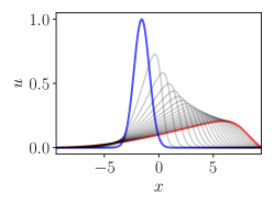
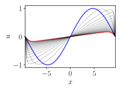
We consider square-integrable solutions to the one-dimensional Burgers equation,
| (1) |
over a domain of length with Dirichlet conditions . Throughout, and which is equivalent to a Reynolds number on a unit-length domain. Three initial conditions will be discussed in the text: a localised Gaussian pulse, , a shifted pulse and a sine wave, : see figure 1.
If the time-forward map of (1) is , then the Koopman operator is defined by
| (2) |
where is a vector made up of observables of the state vector which simply could just be one functional of evaluated at different . A Koopman eigenfunction is a special observable for which ( being the eigenvalue) and (assuming completeness) the set of all Koopman eigenfunctions can be used to represent and time-advance a vector of observables, as follows
| (3) |
where are the (vector) Koopman modes specific to the vector of observables under consideration. The apparent linearity in this expansion is a consequence of the coordinates; in general an individual mode, cannot be considered in isolation. For example, if is defined as simply evaluated at different values, is not a (discretized) solution of the governing equation (1).
For nonlinear systems the requirements for DMD and Koopman analysis to overlap are challenging in practice to enforce. In linear systems, however, the Koopman eigenfunctions are linear functionals of the state and DMD with the full state variable will yield all of the Koopman modes (Rowley and Dawson, 2017). Fortunately, the well-known Cole-Hopf transformation (Hopf, 1950; Cole, 1951)
| (4) |
where converts Burgers equation for with into the simple diffusion equation for with . The utility of the Cole-Hopf transform in the context of a Koopman analysis was noted in Kutz et al. (2016b). As described below, it can be leveraged to obtain Koopman eigenfunctions due to the fact that can be treated as an array of observables (functionals of ) parameterized by whose evolution is governed by a linear equation. Since the diffusion equation is highly tractable, an analytical spectral analysis of the associated Koopman operator is possible.
A Koopman mode expansion of takes the form
| (5) |
where the dependence on (via the Koopman eigenfunctions ) and (via the Koopman modes ) is separated. Given by definition and the linearity of the diffusion equation, the Koopman modes have to be eigenfunctions of the 1D Laplacian. This together with the boundary conditions means that the only possibility is that ( even) or ( odd). The Koopman eigenfunctions required to evolve are then
| (6) |
where , so that the observable can be evolved in time as follows: , with the Koopman eigenvalues .
Now the strategy is to leverage knowledge of the expansion (5) by exploiting the Cole-Hopf transformation to perform a Koopman analysis of . We write
| (7) |
using different symbols for the Koopman eigenfunctions () and eigenvalues () here since an expanded set (which includes the and defined in equation (6) ) will be required. At time , the Cole-Hopf transformation in the form reads
| (8) |
which allows the Koopman eigenfunction and Koopman mode pairs to be determined from the recurrence relation
| (9) |
where , and by inspection, the Koopman eigenvalues are .
The Koopman eigenvalues and the first eight non-zero modes (evaluated with initial condition ) are reported in figure 2 (the neutral mode is just which is the only smooth equilibrium possible in the current configuration (Benton and Platzman, 1972)). Analytical expressions for the first eight non-trivial pairs are
| (10a) | ||||
| (10b) | ||||
| (10c) | ||||
| (10d) | ||||
| (10e) | ||||
| (10f) | ||||
| (10g) | ||||
| (10h) | ||||

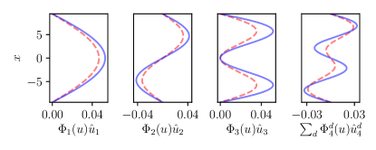
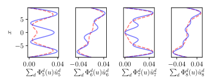
Equations (10d-g) indicate that the Koopman eigenvalues of Burgers equation are degenerate, and that the degree of degeneracy increases with the mode number. Of the modes reported above, numbers through are 2-fold degenerate while mode is 3-fold degenerate. Continuing upwards in mode number, it can be shown that mode is 4-fold degenerate (, and the corresponding eigenfunctions are ). The cause of the degeneracy is connected to the fact that if and are Koopman eigenfunctions with respective eigenvalues and , then is also a Koopman eigenfunction with eigenvalue (Mezić, 2013). Since the linear dynamics of are governed by a simple diffusion, the associated eigenvalues are those of the Laplacian and are proportional to perfect squares. Therefore, the eigenvalue will be -fold degenerate, where is the number of ways the perfect squares can be combined to give . In fact, it has been proved recently that asymptotically (where is a positive constant) (Vaughan, 2015) and so grows very quickly with .
Despite the ubiquity of the Laplacian, this eigenvalue degeneracy is not generic since a more general evolution operator based on a Laplacian will also contain other terms which will disrupt the ordered distribution of the eigenvalues. For example, in the Navier-Stokes equations, the presence also of advection terms is enough to prevent this degeneracy. However, there is also reason to believe this degeneracy occurs in other nonlinear PDEs and so is not unique to Burgers either. For example, the KdV equation can be solved via an inverse scattering transform (Drazin and Johnson, 1989). As part of this procedure, the initial condition on is treated as a potential from which scattering data are derived. The scattering data (a set of observables) can be evolved linearly in time before the inverse scattering transform is used to infer the state variable at later times. This procedure yields a subset of the Koopman eigenvalues. For the classic -soliton solution, these eigenvalues are proportional to the perfect cubes, allowing for the emergence of degeneracy in a manner analogous to Burgers equation.
The degeneracy in Burgers equation has important consequences for interpreting the results of DMD since a data set derived from a single initial condition can only carry information about one realization from the multi-dimensional eigenspace associated with the eigenvalue. This means the dynamic mode which emerges from applying DMD will be initial-condition dependent contrary to usual expectations. This point is illustrated in figure 2, where the Koopman modes (summed over their degeneracies) associated with the shifted initial condition are overlaid onto those obtained with . For the non-degenerate modes () the result is a trivial rescaling whereas for the degenerate modes , the shape functions are altered significantly. To circumvent this issue, DMD would have to treat data from at least different initial conditions to have any chance of properly sampling the -dimensional eigenspace of a degenerate Koopman eigenvalue.
The Koopman expansion for is a decomposition of the solution of a nonlinear PDE into a superposition of fixed nontrivial coherent structures with simple (exponential) temporal behaviour, but it would be a mistake to conclude that a Koopman mode has dynamical significance in isolation. They are not individually solutions to (1) and generally it is not possible to set up an initial condition which only excites a single Koopman mode. For example, while the initial condition can be expressed solely in terms of the second Koopman mode, , their time evolutions do not match. This is because the associated eigenfunction 111Initial conditions invariant under require only a subset of to describe their evolution. so has to be expressed using an infinite sum of all the other Koopman modes. Moreover, the Koopman modes are linearly dependent: compare the Koopman mode associated with (10b) to the second Koopman mode associated with the 2-fold degenerate (10d). This linear dependence has important consequences for interpreting the results of DMD which are often used to build a low-dimensional model of the dynamics (e.g. Kutz et al., 2016a). Normally a least-squares fit is performed on a subset of DMD modes to a snapshot of the system but this is clearly inappropriate for a linearly dependent set of Koopman modes. Correct ‘fitting’ can only be guaranteed by evaluating the Koopman eigenfunctions , which uniquely determine the amplitudes of the Koopman modes.
If the Koopman mode expansion in (7) is to be used to evolve forward in time, a large number of Koopman modes may need to be accurately resolved. In fact, for both and , the Koopman eigenfunctions decay only very slowly as (sharp -variations at translate into a large number of Koopman modes in ). The near-continuum of distinct timescales (the dense eigenvalues in figure 2) also renders selection of the adjustable parameters in DMD difficult (time window length, snapshot spacing and potentially a rank truncation of the data matrix). In general, these selection issues require one to focus on a particular timescale of interest – e.g. in run-down Burgers’ calculations, the focus may be on the most slowly decaying Koopman modes 222At large times, and .
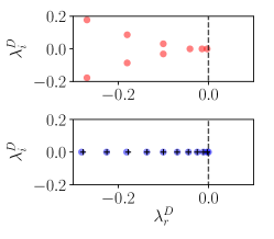
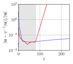
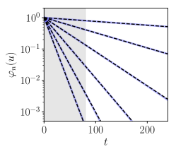
As way of illustration, the output of a DMD of the propagating and decaying Gaussian pulse, , is reported in figure 3 (using the algorithm in (Tu et al., 2014)). The data was obtained from numerical solution of Burgers’ equation using an expansion in Chebyshev polynomials (hence the state vector , where ). Two observables are considered: the raw state vector and the linearizing observable . Clearly, the eigenvalues in the former case do not match the analytical solution which are all on the negative real axis (the displacement of the eigenvalues from the negative real axis shares qualitative similarities with DMD results reported in Bagheri, 2013). There is also a rapidly growing error when the DMD approximation is advanced beyond the observation window. In this case, the failure to resolve the Koopman eigenfunctions means that DMD here amounts to an elaborate curve fitting exercise.
The calculation performed with the observable is an example of EDMD (Williams et al., 2015). Here, the elements of the observable vector constitute a suitable basis for the eigenfunctions and thus DMD successfully extracts the exact decay rates for the linearizing observable . However, note that the full state vector cannot be expressed solely in terms of these eigenfunctions, and so the EDMD algorithm would fail to extract Koopman modes for without further augmentation of . Instead, the Cole-Hopf transform is applied to a superposition of EDMD modes for to obtain the -evolution, and the correct identification of the slow Koopman modes for is highlighted in figure 3 via the agreement between this approximation and the original trajectory far beyond the observation window. In addition, figure 3 also includes a comparison of the DMD approximation to the first few Koopman eigenfunctions (, where is the left-eigenvector of the DMD operator) to the analytical result. Again, excellent agreement is observed far beyond the observation window. However, note that the practical issue highlighted above applies here: while the parameters of the DMD were sufficient to recover the slow dynamics of the system, the failure to resolve the rapidly decaying Koopman modes is apparent in the significant error at early times (middle plot of figure 3).
In this communication we have analytically derived the full Koopman mode and eigenfunction decomposition for Burgers equation – the first time this has been done for a nonlinear PDE. This has provided a nice example of how different sets of Koopman eigenfunctions are needed to propagate different observables (e.g. compare the set of Koopman eigenvalues for and ). It has also revealed Burgers equation as an accessible nonlinear PDE in which the Koopman eigenvalues are highly degenerate and Koopman modes can be linearly dependent. This system, therefore, should prove an invaluable testing ground for the refinement of DMD/Koopman schemes designed to tackle these subtleties in more complex systems.
Acknowledgements: This work was funded by EPSRC under grant EP/K034529/1. The authors thank T. Wooley for bringing (Vaughan, 2015) to their attention and the referees for their helpful comments which improved the manuscript.
References
- Koopman (1931) B. O. Koopman, Proc. Nat. Acad. Sci. 17, 315 (1931).
- Mezić (2005) I. Mezić, Nonlinear Dynam. 41, 309 (2005).
- Schmid (2010) P. J. Schmid, J. Fluid Mech. 656, 5 (2010).
- Bagheri (2013) S. Bagheri, J. Fluid Mech. 726, 596 (2013).
- Jovanović et al. (2014) M. R. Jovanović, P. J. Schmid, and J. W. Nichols, Phys. Fluids 26, 024103 (2014).
- Kutz et al. (2016a) J. N. Kutz, S. L. Brunton, B. W. Brunton, and J. L. Proctor, Dynamic Mode Decomposition: Data-Driven Modeling of Complex Systems, 1st ed. (SIAM, 2016).
- Rowley et al. (2009) C. W. Rowley, I. Mezić, S. Bagheri, P. Schlatter, and D. S. Henningson, J. Fluid Mech. 641, 115 (2009).
- Tu et al. (2014) J. H. Tu, C. W. Rowley, D. M. Luchtenburg, S. L. Brunton, and J. N. Kutz, J. Comput. Dynam. 1, 391 (2014).
- Rowley and Dawson (2017) C. W. Rowley and S. T. M. Dawson, Ann. Rev. Fluid Mech. 49, 387 (2017).
- Sharma et al. (2016) A. S. Sharma, I. Mezić, and B. J. McKeon, Phys. Rev. Fluids 1, 032402(R) (2016).
- Arbabi and Mezić (2017) H. Arbabi and I. Mezić, Phys. Rev. Fluids 2, 124402 (2017).
- Williams et al. (2015) M. O. Williams, I. G. Kevrekidis, and C. W. Rowley, J. Nonlinear Sci. 25, 1307 (2015).
- Brunton et al. (2016) S. L. Brunton, B. W. Brunton, J. L. Proctor, and J. N. Kutz, PLoS ONE 11 (2016).
- Hopf (1950) E. Hopf, Commun. Pure Appl. Math. 3, 201 (1950).
- Cole (1951) J. D. Cole, Quart. Appl. Math. 9, 225 (1951).
- Kutz et al. (2016b) J. N. Kutz, J. L. Proctor, and S. L. Brunton, arXiv 1607.07076 (2016b).
- Benton and Platzman (1972) E. R. Benton and G. W. Platzman, Quart. Appl. Math. 30, 195 (1972).
- Mezić (2013) I. Mezić, Ann. Rev. Fluid Mech. 45, 357 (2013).
- Vaughan (2015) R. C. Vaughan, Int. J. Number Theory , 1 (2015).
- Drazin and Johnson (1989) P. G. Drazin and R. S. Johnson, Solitons: an introduction, 1st ed. (Cambridge University Press, 1989).
- Note (1) Initial conditions invariant under require only a subset of to describe their evolution.
- Note (2) At large times, and .