Fragmentation Uncertainties in Hadronic Observables for Top-quark Mass Measurements

  Abstract  

We study the Monte Carlo uncertainties due to modeling of hadronization and showering in the extraction of the top-quark mass from observables that use exclusive hadronic final states in top decays, such as $t\to\text{anything+J/$\psi$}$ or $t\to\text{anything}+(B\to\text{charged tracks})$, where $B$ is a $B$-hadron. To this end, we investigate the sensitivity of the top-quark mass, determined by means of a few observables already proposed in the literature as well as some new proposals, to the relevant parameters of event generators, such as HERWIG 6 and PYTHIA 8. We find that constraining those parameters at $\mathcal{O}(1\%-10\%)$ is required to avoid a Monte Carlo uncertainty on $m_{t}$ greater than 500 MeV. For the sake of achieving the needed accuracy on such parameters, we examine the sensitivity of the top-quark mass measured from spectral features, such as peaks, endpoints and distributions of $E_{B}$, $m_{B\ell}$, and some $m_{T2}$-like variables. We find that restricting oneself to regions sufficiently close to the endpoints enables one to substantially decrease the dependence on the Monte Carlo parameters, but at the price of inflating significantly the statistical uncertainties. To ameliorate this situation we study how well the data on top-quark production and decay at the LHC can be utilized to constrain the showering and hadronization variables. We find that a global exploration of several calibration observables, sensitive to the Monte Carlo parameters but very mildly to $m_{t}$, can offer useful constraints on the parameters, as long as such quantities are measured with a 1% precision.

1 Introduction

The top quark mass ($m_{t}$) is a fundamental parameter of the Standard Model which, together with the $W$ mass, constrained the Higgs mass even before its discovery. It plays a crucial role in the determination of the Standard Model vacuum life-time, which has been recently found to be at the border between stability and metastability [1, 2]. It is therefore of paramount importance to measure $m_{t}$ with the highest possible accuracy and provide a reliable determination of the error on $m_{t}$. Furthermore, much work has been lately carried out in order to estimate the uncertainty on $m_{t}$, once it is interpreted in terms of well-defined theoretical quantities, such as the pole mass [3, 4, 5].

In fact, standard measurements, based on the template, matrix-element and ideogram methods (see, $e.g.$, the analyses in [6, 7, 8]), rely on parton shower generators such as HERWIG [9] or PYTHIA [10]. They simulate the hard scattering at leading order (LO) and multiple radiation in the soft or collinear approximation, with phenomenological models for hadronization and underlying events. By contrast, so-called alternative methods use other observables, e.g., total cross sections or kinematic endpoints, which, besides Monte Carlo simulations, can be compared directly with fixed-order and possibly resummed QCD calculations, thus allowing a straightforward theoretical interpretation of the extracted mass (see, for example, Ref. [11] on the pole mass extraction from the total $t\bar{t}$ production cross section).

More recent NLO+shower programs such as aMC@NLO [12] and POWHEG [13] implement NLO hard-scattering amplitudes, but still rely on HERWIG and PYTHIA for parton cascades and non-perturbative phenomena. NLO corrections to top quark production have been available in both aMC@NLO and POWHEG for some time, while much effort has been later devoted to improve the treatment of top quark decays. In the aMC@NLO code, NLO top decays are implemented for single-top events [14]; in $t\bar{t}$ production, the decays are still on shell, but spin correlations and part of the off-shell contributions are included via MadSpin [15]. In the POWHEG framework, NLO corrections to top decays were implemented first in Ref. [16], with an approximate treatment of top-width effects, and more recently, in Ref. [17], the interference between top production and decay, as well as non-resonant contributions have been included. Furthermore, the SHERPA code [18] implements $t\bar{t}$ production in conjunction with up to three jets at NLO, merged to parton showers along the lines of Ref. [19]. Top decays in SHERPA include spin correlations and are accounted for in the LO approximation [20].

At present, since most standard $m_{t}$ determinations rely on the reconstruction of $b$-flavored jets in top decays ($t\to bW$), one of the main uncertainties is from the $b$-jet energy scale (bJES), which amounts to about 250 MeV of the overall 700 MeV in the world average determination [21]. Therefore, several attempts have been made so far to overcome the difficulties of such standard methods, in particular to calibrate the jet energies to very high accuracy. Some strategies use the $W$-boson mass as a constraint to calibrate in-situ the jet reconstruction [7]: this method, however, cannot account for the differences between $b$-jets and light-flavored jets, as the $W$ decays mostly into light or charm quarks. In other attempts the jet energy scale has been effectively constrained by exploiting the anti-correlation of the $b$-jet energy and angular variables [8] imposed by the $V-A$ matrix element that in the Standard Model describes top-quark decay.

Despite all these efforts, the jet energy scale keeps being a bottleneck for the improvement of standard mass measurements; therefore, new methods have been conceived to go around this uncertainty. Among the earliest attempts, we recall those based on the exclusive fragmentation of the $b$-quark to $J/\psi$ [6, 22] and studies of the decay length of $B$ hadrons [23, 24]. In the $J/\psi$ method, leptonic decays of the $J/\psi$ are used to identify the resonance. The distribution in the invariant mass formed by the two leptons from the $J/\psi$ and the lepton from $W$ decay, $m_{\ell\bar{\ell}\ell^{\prime}}$, is the key observable which is then compared with a set of Monte Carlo simulation samples generated with different input top quark masses. The overall strategy does not directly involve any jet-energy measurement in the determination of the quantity sensitive to the top quark mass, and therefore it is free from jet-energy calibration issues. Similarly, the determination of the $B$ hadron decay length does not involve directly any jet-energy measurement, as it is based on the identification of the secondary vertex in the event through tracking: therefore, this measurement is clean from jet-calibration issues.

For all methods involving the tagging of exclusive hadronic final states, e.g., the di-lepton $J/\psi$ final state mentioned above, we expect the following number of recorded events at 14 TeV LHC:

$$N_{\text{ev}}\sim 10^{5}\frac{\mathcal{L}}{1\text{ab}^{-1}}\frac{\epsilon_{\text{tagging}}}{10^{-4}}\cdot\epsilon_{\text{cuts}}\cdot BR(t\bar{t})\,,$$ (1)

where $\mathcal{L}$, $\epsilon_{\text{tagging}}$, $\epsilon_{\text{cuts}}$, and $BR(t\bar{t})$ denote the integrated luminosity in ab^-1, the tagging efficiency for hadronic objects of interest, the fraction of events satisfying the associated selection cuts, and the branching ratio of $t\bar{t}$ into a given final state, respectively.

For the $J/\psi$ clean di-lepton tagging, $\epsilon_{\text{tagging}}$ will be ${\cal O}(10^{-5})$, just taking into account branching fractions. Adding up all decay modes of $B$ hadrons that can be reconstructed from just charged tracks (e.g., $B^{+}\to K^{+}\pi^{+}\pi^{-}$), we may increase the number of events by a factor ${\cal O}$(1-10). Therefore we adopt $\epsilon_{\text{tagging}}\sim 10^{-4}$ as baseline in eq. (1). Clearly these methods face the challenge of collecting the sufficient number of events in order to fulfill precision mass measurements; for $\epsilon_{\text{cuts}}\cdot BR(t\bar{t})\lesssim 1$ and an integrated luminosity of several ab^-1, the desired statistics may nevertheless be reached [25]. Although not being affected by uncertainties from jet measurements, in the $J/\psi$ analysis a crucial role is nevertheless played by the hadronization of $b$ quarks into $B$-hadrons and the associated Monte Carlo uncertainty. Reference [25] estimates that the contribution due to bottom-quark fragmentation is about 300 MeV, for a total theoretical error of 900 MeV

In case of less exclusive requirements on $B$-hadron decays, it is possible to obtain larger data samples. This would be the case, for instance, of an analysis based on $B\to\ell+X$, which may allow to extract $m_{t}$ from the $m_{\ell\ell}$ distribution obtained by pairing up the soft lepton from $B$ decay and the lepton from the $W$ boson in the same top-quark decay. This method has been employed by CDF [26] and might be used in LHC data as well.

Exactly as it is the case for mass measurement from the $J/\psi$ method, in a mass determination that uses soft leptons from $B$ hadrons, we should expect a sensitivity to the showering and hadronization description of the event and corresponding systematics. A similar conclusion holds for methods that use the decay length of $B$ hadrons [23, 24] and those that exploit the mass of the secondary vertex from charged particles [27]. It is the purpose of this work to study the hadronization uncertainties that affect all these methods.

Understanding the transition of $b$ quarks into $B$ hadrons is a crucial step to correctly predict the observables involved in the above-described mass measurements. This aspect of the physics of quarks and hadrons is ruled by non-perturbative QCD and it is clearly a challenge to describe it accurately starting from first principles. One possibility to fill in this gap is to advocate a factorization of long-distance effects, namely the hadronization mechanism, from the hard-scattering events. In this way it is possible to measure from data a non-perturbative fragmentation function $D_{H,q}(z)$, accounting for the transition of a quark $q$ into a hadron $H$, carrying an energy fraction $z$. Most precise measurements of these fragmentation functions have been obtained at LEP [28, 29] and SLD [30] experiments from which it is possible to obtain $D_{H,q}(z)$ at an energy scale $Q^{2}$ of the order of the inelasticity of the reaction. For processes $e^{+}e^{-}\to b\bar{b}$ at the LEP, it is $Q^{2}\simeq m_{Z}^{2}$: once known at some $Q^{2}$, the fragmentation functions can be evolved to different $Q^{2}$ by means of perturbative evolution equations, analogous to those used for parton distribution functions.

Bottom-quark fragmentation is usually described using the perturbative-fragmentation formalism [31]: up to power corrections ${\cal O}(m_{b}^{2}/Q^{2})$, the heavy-quark spectrum can be factorized as a massless coefficient function and a process-independent perturbative fragmentation function, associated with the transition of a massless parton into a heavy quark. Such an approach allows a straightforward resummation of the large mass $\ln(m_{b}^{2}/Q^{2})$ and threshold contributions, $\sim[1/(1-z)]_{+}$ and $\sim[\ln(1-z)/(1-z)]_{+}$, which become large for $z\to 1$, corresponding to soft- or collinear-gluon radiation. In the perturbative-fragmentation approach, the state of the art is next-to-leading-order (NLO) accuracy in $\alpha_{S}$, with next-to-leading logarithmic (NLL) resummation: Refs. [32, 33, 34] apply this formalism for bottom fragmentation to $e^{+}e^{-}-$ annihilation, top and Higgs decays, respectively. Heavy-hadron spectra are then obtained by convoluting the heavy-quark energy distribution with non-perturbative fragmentation functions, such as the Kartvelishvili [35] or Peterson [36] models, containing few parameters which must be tuned to experimental data.

More recently, the approach based on Soft Collinear Effective Theory (SCET) and Heavy Quark Effective Theory (HQET) was used in the NNLO+NNNLL approximation in order to determine the $b$-quark fragmentation function from $e^{+}e^{-}$ annihilation at the $Z$ pole [37]. The authors found a general good agreement with the data, although some discrepancy is still present for large values of the energy fraction, where one is mostly sensitive to non-perturbative effects.

Although having lately become very accurate, calculations based on the fragmentation-function formalism are nonetheless too inclusive for a complete description of the final states and in general they need to be performed independently for each observable and hard-scattering reaction. Moreover, this approach is based on factorization, so it is not obvious whether the non-perturbative fragmentation function measured in a color-neutral environment, such as $e^{+}e^{-}$ machines, could be straightforwardly extended to colored parton scatterings at hadron colliders.

As an alternative to the fragmentation function approach, there have been attempts to describe the formation of hadrons with phenomenological models inspired by some features that can be derived from first principles, albeit depending on a few parameters; namely the string model [38, 39] or the cluster model [40]. This sort of approach is most common in shower Monte Carlo event generators, which are usually shipped with a “tuning” of the phenomenological parameters in such a way that they are tailored to reproduce a large set of previously available data like $e^{+}e^{-}\to{\rm hadrons}$. This approach is based on the universality of the hadronization transition, which, in principle would allow one to use models tuned at $e^{+}e^{-}$ machines even at hadron colliders. However, as discussed above, it is not guaranteed that they will still be reliable in a colored environment, wherein even initial-state radiation and underlying event will play a role. Furthermore, the number of parameters involved is usually quite large, especially in the string model, and there is no clear factorization between perturbative and non-perturbative physics: every time one tries to tune a specific sample of experimental data, one should be warned that the possible agreement with other data may be spoiled.

Moreover, when using fragmentation functions and hadronization models, it is hard to make a reliable estimate of theory uncertainties. In general, there are pitfalls in carrying the properties of $e^{+}e^{-}$ measurements to hadronic machines; although it is assumed that they will be accurate enough to capture correctly effects of order $\Lambda_{QCD}$, the evaluation of the systematics due to this assumption is difficult to assess. For this reason it would be desirable to determine the hadronization parameters directly in hadronic collisions, so to remove all the issues tied with the use of $e^{+}e^{-}$ data.

Extracting accurate fragmentation functions at hadronic colliders might bring about a formidable task. In fact, one needs to overcome the difficulty to obtain precise data and match them with sufficiently accurate theory calculations. For the purpose of top-quark phenomenology, this will likely need an NNLO accuracy in order not to spoil a sub-GeV accuracy on the top-quark mass determination. Furthermore, the complexity of reconstructing the top-quark rest frame impedes the direct measurement of energy-fraction variables such as the $x_{B}=2\cdot E_{B}/\sqrt{s}$ measured at LEP and SLD experiments, where the $Z$ rest frame coincides with the laboratory frame.

The use of hadronization models for precision physics at hadron colliders is challenging because simple models have had hard time to reproduce accurate experimental results [43, 44, 45] and elaborate models with many parameters are needed to describe $e^{+}e^{-}\to hadrons$ data. The large number of phenomenological parameters needed to describe present data makes it difficult to find a unique favorite set that best reproduces them. Even if such “best fit” point is found (or hand-picked), it is often the case that the determination of each parameter is tied to that of the others contained in the model. Such a non-trivial correlation makes it hard to evaluate the impact on physical observables of the change of each parameter, hence to define a theory uncertainty due to the modeling of hadronization.

A further complication arises from the fact that any hadronization model is strictly related to the the parton cascade, hence even the non-perturbative parameters are closely entangled with those characterizing the shower. All of this shows that it is necessary to carry out a coordinated study to constrain both hadronization and shower parameters from data, including possible $pp\to t\bar{t}$ samples, in order to feel confident with the fits and their possible use in other environments. This was the purpose of the tunes of the PYTHIA 8 generator, such as the Monash tune [46], which we will take as baseline for our study, and of the efforts in the ATLAS collaboration [47] towards adding $t\bar{t}$ data in the fits.

Color reconnection is another source of non-perturbative uncertainty in $m_{t}$, accounting for about 300 MeV in the estimate of the error in the world-average analysis [21]. Although color reconnection can even take place, e.g., in $e^{+}e^{-}\to WW\to 4$ jets processes at $e^{+}e^{-}$ colliders, events where bottom quarks in top quark decays are color-connected to initial-state antiquarks do not have their counterpart in $e^{+}e^{-}\to b\bar{b}$ annihilation. Therefore, color reconnection in $t\bar{t}$ events should deserve further investigation and may even need Monte Carlo retuning at hadron colliders. Studies on the impact of color reconnection on $m_{t}$ were undertaken in Refs. [48, 49], in the frameworks of PYTHIA and HERWIG, respectively. Ref. [48] investigated the description of color reconnection within the PYTHIA string model, finding that, even restricting to the most sophisticated models, it can have an impact up to 500 MeV on the top mass. On the other hand, Ref. [49] addressed this issue by simulating fictitious top-flavored hadrons in HERWIG and comparing final-state distributions, such as the $BW$ invariant mass, with standard $t\bar{t}$ events. In fact, assuming that top-flavored hadrons decay according to the spectator model, the $b$ quark is forced to connect with the spectator or with antiquarks in its own shower, so that color reconnection with the initial state or with $\bar{t}$-decay products is suppressed.

In this work we study the impact of the hadronization model parameters on precision measurements of the top-quark mass, for which a target accuracy around 0.5% is set. The aimed accuracy is about the uncertainty where current most precise measurements of $m_{t}$ tend to accumulate, mainly because of the limited knowledge of the jet energy. As the study of $B$-hadrons is motivated by going beyond the present limitations, this is clearly the precision level that hadronic observables need to reach in order to be useful. This accuracy corresponds to an absolute error $\delta m_{t}\simeq\Lambda_{\rm QCD}$, which for hadronic observables implies the necessity to carefully model hadronization effects, whose impact on the single $B$-hadron kinematics is naturally of the same order of magnitude as $\Lambda_{\rm QCD}$.

In the following, we study several observables that have been discussed in the literature to measure the top mass, and assess the error on $m_{t}$ that would stem from a variation of hadronization and related shower parameters. As some of these observables have been proposed in studies of $b$-jets, we will define analogous variables for single $B$-hadrons: for example, a measurement of the invariant mass $m_{bl}$ of the $b$-tagged jet and a charged lepton has been modified to the invariant mass formed by the $B$-hadron and a charged lepton. For each observable, we derive the sensitivity of the top quark mass to the parameters of hadronization and showering. We then collect results in the tables of the following sections, expressing them in terms of logarithmic derivatives like:

$$\Delta_{\theta}^{(O)}\equiv\frac{\bar{\theta}}{\bar{O}}\frac{\partial O}{\partial\theta},$$ (2)

where $O$ is a generic observable in $t\bar{t}$ events, the bar in $\bar{O}$ and $\bar{\theta}$ indicates an average value in a given range, and $\theta$ denotes a generic Monte Carlo hadronization or showering parameter. While studying these sensitivities, we shall compute the precision in the knowledge of the value of these parameters that is necessary to achieve in order to warrant a sub-GeV theoretical error on the $m_{t}$ determination from hadronic observables.

Furthermore, we carry out similar studies to quantify the sensitivity to showering and hadronization parameters of observables that are not sensitive to the top-quark mass. We henceforth name these quantities “calibration observables” which are useful to gauge the suitability of the tunes obtained elsewhere to describe hadronization in the top-quark specific context. As the calibration observables do not (or very mildly) depend on $m_{t}$, the measurements of these observables can be used to constrain the showering and hadronization parameters that have the greatest impact on the observables sensitive to $m_{t}$, thus resulting in an improvement of the accuracy and the robustness of the mass measurement. A combined determination from data of both $m_{t}$ and Monte Carlo variables could be called an “in situ” calibration of the nuisance theoretical parameters that affect the top-quark mass determination with hadronic observables. In a way this could be thought as a strategy similar to the in-situ calibration of the jet-energy correction obtained from the reconstruction of the hadronic $W$ boson peak in top quark events of Ref. [51]. Here, of course, we would be calibrating parameters of the phenomenological hadronization models and of the parton shower. The use of $N+1$ observables, where $N$ are mostly sensitive to Monte Carlo parameters and one is mostly sensitive to $m_{t}$, could be considered as an ultimate strategy for the top quark mass determination or for the cross-check of theoretical uncertainties in the global picture of top quark mass determinations at the Large Hadron Collider. In the following, combining the results on calibration observables and mass sensitive ones, we will outline the ingredients and the inherent difficulties of such analysis.

To deliver our ideas efficiently, the paper is organized as follows. In Section 2, we begin with identifying relevant hadronization and shower parameters in PYTHIA 8 and HERWIG 6, together with their variation ranges to compute associated sensitivities. We then discuss kinematic observables to be used throughout this paper and the reconstruction schemes for the variables carrying some subtlety in Section 3. Section 4 is devoted to reporting our results on the calibration observables, while we present our analysis on observables sensitive to $m_{t}$ in Section 5. Our conclusions and outlook will be presented in Section 6. Finally, two appendices are reserved for discussing some details of our computation.

2 Parameters and calculations

Hereafter we shall study the process

$$pp\to t\bar{t}\to\ell^{-}\ell^{+}b\bar{b}\bar{\nu}\nu,$$ (3)

using PYTHIA 8.2 [10] or HERWIG 6 [9], namely LO hard scattering, parton showers and hadronization according to the string [38, 39] or cluster [40] models, respectively. In the simulation of $t\bar{t}$ events, standard HERWIG and PYTHIA factorize production and decay phases and the top-quark width is neglected. Such effects are included in the new $b\bar{b}4\ell$ generator [17], implemented in the framework of the POWHEG-BOX [13], which simulates the full $pp\to b\bar{b}\ell^{+}\ell^{-}\nu_{\ell}\bar{\nu}_{\ell}$ at NLO, including the interference between top production and decay, as well as non-resonant contributions. Investigations of width effects and full NLO corrections to top decays are nevertheless beyond the scopes of the present paper and we defer it to future explorations. We point out, however, that both HERWIG and PYTHIA implement matrix-element corrections to parton showers in top decays, along the lines of [52] and [53], respectively, and therefore hard- and large-angle gluon radiation in $t\to bW$ processes will be taken into account in the results which we will present hereafter.

2.1 Variation of PYTHIA parameters

In order to reproduce the data, a number of hadronization parameters can be tuned; some of them are specific to heavy flavors and the formation of $B$ hadrons, while others are meant to describe hadronization of light flavors. In our study we concentrate on heavy-flavor parameters and study variations of the Lund string model $a$ and $b$, by considering deviations from the best-fit values which are used to describe light-flavored hadrons. Furthermore, we will also vary the $r_{B}$ parameter, the Bowler modification of the fragmentation function for massive quarks, which reads [39]:

$$f_{B}(z)\sim{1\over{z^{1+b\,r_{B}m^{2}_{q}}}}(1-z)^{a}\exp\left(-\frac{b\,m_{T}^{2}}{z}\right).$$ (4)

Here the $z$ variable implies the fraction of $E+p_{z}$ taken by the $B$ hadron under the assumption that a $b$ quark of energy $E$ moves along the $z$-axis, while $m_{T}$ symbolizes the associated $B$-hadron transverse mass.

As discussed in the introduction, hadronization models are specific to the showering to which they are attached, and therefore it is important to study the sensitivity of top-mass observables to variations of the showering quantities. Parameters for which a sensitivity is expected include $p_{T,\text{min}}$ which is the scale at which the parton shower is stopped and hadronization models take over, the value of the strong coupling constant at the $Z$-boson mass that is used in the final-state parton shower, and the value of the $b$ quark mass. In addition, we also check the effect induced by discrete choices in using the $b$-quark or the $W$ boson as a recoiler to impose momentum conservation when we have splittings from the $b$ quark in the shower.

It is important to remark that the chosen range of variation of these parameters has little importance for the calculation of the sensitivity defined in eq. (2). In fact, the derivative of the observables with respect to the Monte Carlo parameters is typically stable across large ranges, and as will be shown later on, even the sensitivity $\Delta_{\theta}^{(O)}$ is largely independent of it. What mainly leads to the choice of given ranges is to have sufficiently large differences between spectra for different parametrizations, so that the derivatives can be computed accurately, without being overwhelmed by the statistical errors due to the finite size of the Monte Carlo sample.

At the same time, we avoid taking values too far from the default, since this might generate unforeseen changes in the Monte Carlo predictions. For these reasons, we shall vary parameters up and down by at most 20% of their central values and evaluate numerically the derivatives in all available data points. For a summary of the PYTHIA parameters and the ranges of variation, we refer to Table 1. In principle, other parameters could be varied and tuned as they affect the kinematics of top quark events. For instance the initial state $\alpha_{s}$ parameter of Pythia8, SpaceShower:alphaSvalue, could be considered. We choose to not investigate them, as they can be fixed from specific measurements such as the jet multiplicity used in [54].

	Pythia8 parameter	range	Monash default
$p_{T,\text{min}}$	TimeShower:pTmin	0.25-1.00 GeV	0.5
$\alpha_{s,\text{FSR}}$	TimeShower:alphaSvalue	0.1092 - 0.1638	0.1365
recoil	TimeShower:recoilToColoured	on and off	on
$b$ quark mass	5:m0	3.8-5.8 GeV	4.8 GeV
Bowler’s $r_{B}$	StringZ:rFactB	0.713-0.813	0.855
string model $a$	StringZ:aNonstandardB	0.54-0.82	0.68
string model $b$	StringZ:bNonstandardB	0.78-1.18	0.98

Table 1: Ranges and central values of the parameters that we varied. Note that some values are not varied around the default values of the Monash tuning. For instance we run $r_{B}$ around the mid-point between Pythia6.4 and Pythia8-Monash values.

2.2 Variation of HERWIG parameters

For the sake of comparison, we also investigate the impact of the HERWIG shower and hadronization parameters on the top-quark mass measurement. In fact, HERWIG and PYTHIA generators differ in several aspects: for example, the ordering variables of the showers are not the same, matrix-element corrections are implemented according to different strategies and, above all, models for hadronization and underlying events are different.

As far as HERWIG is concerned, hadronization occurs according to the cluster model, which is strictly related to the angular ordering of the parton shower, yielding color pre-confinement even before the hadronization transition. In the following, we shall use the HERWIG 6 event generator, written in Fortran language. In fact, the object-oriented code HERWIG 7 [55] presents a number of improvements, especially when using the new dipole shower model with the modified kinematics for massive quarks [56]. However, although the latest version HERWIG 7.1 exhibits remarkable improvements for the purpose of bottom-quark fragmentation, the comparison with the $e^{+}e^{-}\to b\bar{b}$ data is still not optimal.

As for HERWIG 6, in Ref. [57] the authors tried to tune it to LEP and SLD data, finding that the comparison could be much improved with respect to the default parametrization, although some discrepancy still persists and the prediction is only marginally consistent with the data. As a whole, we decided to follow [57] and stick to using HERWIG 6 in the present paper. As done in the case of PYTHIA, we identify the relevant shower and hadronization parameters and vary them by at most 20% around their respective default values.

The relevant parameters of the cluster model are the following: CLMSR(2) which controls the Gaussian smearing of a $B$-hadron with respect to the $b$-quark direction, PSPLT(2) which governs the mass distribution of the decays of $b$-flavored clusters, and CLMAX and CLPOW which determine the highest allowed cluster masses. Their default values and variation ranges are summarized in Table 2. Furthermore, unlike Ref. [57] which just accounted for cluster-hadronization parameters, we shall also explore the dependence of top-quark mass observables on the following parameters: RMASS(5) and RMASS(13), the bottom and gluon effective masses, and the virtuality cutoffs, VQCUT for quarks and VGCUT for gluons, which are added to the parton masses in the shower (see Table 2). We also investigate the impact of changing QCDLAM as it plays the role of an effective $\Lambda_{\rm QCD}$ in the so-called Catani–Marchesini–Webber (CMW) definition of the strong coupling constant $\alpha_{S}$ in the parton shower (see Ref. [58] for the discussion on its relation with respect to the standard $\Lambda_{\rm QCD}$ in the $\overline{\rm MS}$ scheme). As well as for other paramters, we vary QCDLAM around its default value, the range of variation is tabulated in Table 2.

	parameter	range	default
Cluster spectrum parameter	PSPLT(2)	0.9 - 1	1
Power in maximum cluster mass	CLPOW	1.8 - 2.2	2
Maximum cluster mass	CLMAX	3.0 - 3.7	3.35
CMW $\Lambda_{QCD}$	QCDLAM	0.16 - 2	0.18
Smearing width of $B$-hadron direction	CLMSR(2)	0.1 - 0.2	0
Quark shower cutoff	VQCUT	0.4 - 0.55	0.48
Gluon shower cutoff	VGCUT	0.05 - 0.15	0.1
Gluon effective mass	RMASS(13)	0.65 - 0.85	0.75
Bottom-quark mass	RMASS(5)	4.6 - 5.3	4.95

Table 2: Herwig 6 parameters under consideration and ranges of their variation.

3 Observables

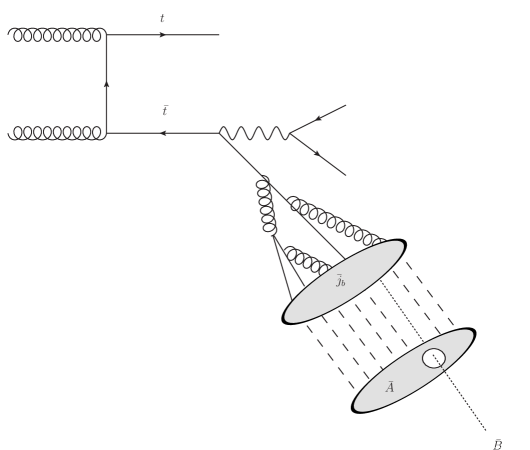
In this section, we identify the observables that we employ to study their sensitivities to parameter variations. We first discuss the observables relevant to top quark mass measurements, followed by our proposed variables for the tuning or the calibration of Monte Carlo parameters. For the formulation of how to compute these observables, we will follow the naming scheme for $t\bar{t}$ final states that we illustrate in Figure 1.

Figure 1: Schematic view of the event, including the transformation of a $\bar{b}$ quark into hadrons, namely into a $\bar{B}$ and other light-flavored hadrons denoted collectively as $\bar{A}$, which together form a $b$-tagged jet $j_{\bar{b}}$. Similarly, a $b$ quark coming from the $t$ gives rise to jets and hadrons denoted by the same symbols without a bar.

3.1 $m_{t}$-determination observables

We first list up the observables that we consider for the top-quark mass measurement.

• $E_{B}$: energy of each tagged $B$-hadron;

• $p_{T,B}$: $B$-hadron transverse momentum;

• $E_{B}+E_{\bar{B}}$ and $p_{T,B}+p_{T,\bar{B}}$: sum of the energies and transverse momenta of $B$ and $\bar{B}$ (in events where both $B$ hadrons are tagged);

• $m_{B\ell}$: invariant mass of the $B$-hadron and one lepton from $W$ decay (the prescription for combinatorial ambiguity arising in forming $m_{B\ell}$ will be discussed shortly);

• $m_{T2}$ [59] and $m_{T2,\perp}$ [60] of the $B$ and the $B\ell$ subsystems defined below;

• $m_{BB\ell\ell}$, the total mass of the system constructed by the two leptons and the two tagged $B$-hadrons in the event.

We choose these observables because some of them have already been discussed in the literature to carry out measurements of $m_{t}$ from hadronic exclusive final states: for instance, $m_{B\ell}$ [41], $m_{T2}$ and its variants [61, 62] and $E_{B}$ [42]. Furthermore, we consider observables that have been discussed for $b$-jets, and can naturally extend them by replacing $b$-jets with $B$ hadrons. For instance, the sum of $B$-hadron energies $E_{B}+E_{\bar{B}}$ is inspired by the analogous $b$-jet quantity $E_{j_{b}}+E_{j_{\bar{b}}}$ defined in [41]. To the best of our knowledge, the variable $m_{BB\ell\ell}$ has not been considered before. It is meant to be sensitive to $m_{t}$ as it probes the the total mass of the $t\bar{t}$ system. Therefore, we expect the bulk of its distribution to be sensitive to the top mass in a way similar to the bulk of the $m_{B\ell}$ distribution. In the lower tail, the variable $m_{BB\ell\ell}$ is anticipated to have sensitivity to the top quark mass because of a threshold effect similar to the one in the proposal of Ref. [63].

It is noteworthy that the observables $E_{B}+E_{\bar{B}}$, $p_{T,B}+p_{T,\bar{B}}$, $m_{BB\ell\ell}$, and all the $m_{T2}$ variables require two tagged $B$-hadrons in each event, and therefore they may be hardly measurable with enough statistics at the LHC. However, it is equally interesting to study them to see how much information on the top quark mass could be present in the kinematics of the whole event, rather than in a single top-quark decay, probed by other observables such as $m_{B\ell}$, $p_{T,B}$, and $E_{B}$. While it may be challenging to secure a sufficient number of events with fully-reconstructed $B$-hadrons, we also remark that for the measurements which do not actually demand tagged $B$-hadron(s), e.g., those based on generic tracks from the secondary vertex, it can be easier to achieve enough statistics. Therefore, our study of these observables with $B$ hadrons is useful to see what can be gained using both sides of the $t\bar{t}$ events in these measurements.

3.1.1 Reconstruction schemes

For observables involving particle pairings, we need to specify a prescription: for example, in order to compute $m_{B\ell}$, we need to choose which lepton should be paired with the tagged $B$ in the event.

Speaking of $m_{B\ell}$ first, we define two variants. In the first one, we pick the lepton that gives the smaller $m_{B\ell}$ for each lepton charge, that is to say, for each event we obtain two values, $\text{min}(m_{B\ell^{+}},m_{B\ell^{-}})$ and $\text{min}(m_{\bar{B}\ell^{+}},m_{\bar{B}\ell^{-}})$, and put both in relevant histograms. This selection scheme enables us to avoid leptons causing an endpoint violation of the true distribution arising from the $B$ and $\ell$ in the same top decay. We call such a computed invariant mass $m_{B\ell,\text{min}}$. We remark that, in the situation in which only one $B$-hadron is identified per event, this simply corresponds to just picking $\text{min}(m_{B\ell^{+}},m_{B\ell^{-}})$. In the second variant of $m_{B\ell,\text{true }}$ we use the event records to pair the $B$-hadron with the lepton that comes from the same top quark as the $B$.

For more complex observables, such as $m_{T2}$, we have to specify further how we deal with constituent particles in the event. The $b$-jet $j_{b}$ is made of the $B$ hadron and some other hadrons that we call $A$, as shown in Figure 1. In a computation of $m_{T2}$ from $b$-jets, we need to calculate the transverse mass in combination with $j_{b}$ and some vector in the transverse plane that stands for one source of missing transverse energy (mET), associated with the neutrino in $W$ decay. When dealing with the $m_{T2}$ of the $B$-hadron, we are naturally led to replace $j_{b}$ by $B$, but this leaves an ambiguity as of what to do with the rest of the jet. The hadrons $A$ in $j_{b}$ are detectable particles, hence not invisible, but at the same time they are extraneous to the $B$-related transverse mass. For this reason, we are allowed to treat them as either extra radiation or invisible particles. In the latter case, they would be added to the mET of the event, as if they were not measured; in the former case, they would be regarded as extra radiation, as some kind of upstream momentum in top-quark decay. We shall call these two variants $m_{T2}^{\text{(mET)}}$ and $m_{T2}^{\text{(ISR)}}$, respectively. For a generic reaction

$$pp\to t\bar{t}\to\ell^{-}\ell^{+}+B+A+\bar{B}+\bar{A}+\bar{\nu}\nu+X,$$

the two options would give rise to mET and ISR computed as in Table 3. In our study, we shall also consider the $m_{T2,\perp}$ variable [60], which was considered at the jet level by CMS in [61]. The variable is defined in a similar fashion to the standard $m_{T2}$, but in the plane perpendicular to the total upstream transverse momentum, so that it is insensitive to ISR, which affects the dynamical details of the $m_{T2}$ spectra. With the $m_{T2,\perp}$ variables, we therefore study the relevant sensitivities in the context of decay kinematics of top quarks, excluding any top quark production-related dynamics.

	mET definition	ISR
$m_{T2}^{\text{(mET)}}$	$\text{mET=}-\sum_{i=\{B,\ell,X\}}\bar{p}_{T,i}$	$X$
$m_{T2}^{\text{(ISR)}}$	$\text{mET}=-\sum_{i=\{A,B,\ell,X\}}\bar{p}_{T,i}$	$X+A+\bar{A}$
$m_{T2}^{\text{(true)}}$	$\text{mET}=-\left(\bar{p}_{T,\nu}+\bar{p}_{T,\bar{\nu}}\right)$	$\sum_{x}$ for x not coming form either $t$ or $\bar{t}$

Table 3: Variants of the reconstruction scheme for $m_{T2}$.

3.1.2 Definition of the sub-system observables

For the computation of the $m_{T2}$ variables it is possible to consider different subsets of top-decay products as visible particles [64]. Barring the light hadrons $A$, each top quark gives rise to a $B$-hadron and a charged lepton $\ell$, with two possible B-hadron-accompanying options for their treatment. We can opt to form a compound system of these two and compute the transverse masses using $p_{B}+p_{\ell}$ as visible momentum or ignore $\ell$ and calculate the transverse mass using the $B$-hadrons and the mET, including the charged leptons as if they were invisible. These two options are labeled:

• “$B\ell$-subsystem” $m_{T2,B\ell}$: the transverse mass is computed from $p_{B}+p_{\ell}$ for some pairing of $B$ and $\ell$ with only the neutrino considered as invisible and the relevant test invisible mass is set to the neutrino mass;

• “$B$-subsystem” $m_{T2,B}$: the transverse mass is computed from $p_{B}$ with the $W$ treated as invisible and the relevant test invisible mass is set to the true $W$ mass.

Both options for $m_{T2}$ yield distributions with a kinematic endpoint at $m_{t}$, hence they can be used to measure the top mass. The “$B$-subsystem” mass $m_{T2,B}$ has the virtue that it does not require any hypothesis on which lepton should be paired with each $B$. The “$B\ell$-subsystem” $m_{T2,B\ell}$, on the contrary, faces the issue of pairing leptons and hadrons, but generally it has the greatest sensitivity to $m_{t}$, especially in the bulk of the distribution, where $m_{T2,B}$ instead exhibits a very mild dependence on $m_{t}$. Overall, the two options offer different pros and cons, making a comparison of their performances rather interesting.

3.2 Calibration observables

Even in presence of a perfect fit to precise $e^{+}e^{-}$ data, there is no guarantee that the Monte Carlo tuning will be a good enough description of LHC data (fragmentation properties of light flavors have proven this to be the case [65]). It is therefore crucial to undertake checks of these tunings specific for light- and heavy-quark physics.

With this motivation in mind, we study “calibration observables”, i.e. quantities that we expect to have no or little sensitivity to $m_{t}$ but still depend on showering and hadronization in $t\bar{t}$ events. Exploiting this feature, one can use these observables to check the accuracy of the tunings or to constrain the Monte Carlo parameters “in-situ” for the mass measurement. In the latter case, the top-quark sample would be used to constrain simultaneously a number of showering and hadronization quantities from the data, as well as $m_{t}$, in the same manner as the jet energy scale in-situ calibration carried out in [51]. We highlight the fact that in this in-situ calibration procedure one may end up with a point of Monte Carlo parameter space that may or may not be close to the point used of the standard tunings, $e.g.,$ the Monash one. The best-fit calibration point, in fact, is very specific to top quark events and in principle even to the selection cuts used to isolate top quarks from background. Therefore, it has a rather different meaning than usual tunings, and we do not expect it to be a Monte Carlo set-up usable outside the domain of the top quark mass measurement.

Furthermore, we point out that our calibration is intended only for the purpose of reducing the impact of fragmentation uncertainties on the $m_{t}$ measurements. For this reason, one might even think of studying the response of the observables to changes in the hadronization model in dijet events with two $b$-tags and better constraining the Monte Carlo parameters: however, this would go in the direction of producing a tuning, rather than an in-situ calibration. In the following, we shall not discuss the use of dijet and other heavy-flavor production processes, but we just leave them as a possible validation of the calibration procedure. Clearly, if a stark deviation from the process-universality of the Monte Carlo parameters had to be observed, this should raise questions on the appropriateness of the theory description employed to model $t\bar{t}$ events and other heavy-flavor production.

Studies to identify observables useful for a calibration specific to top quark have been carried out by ATLAS in the tuning work [47], as well as in Ref. [66]. These investigations consider the observables:

• $p_{T,B}/p_{T,j_{b}}$: the ratio of the $B$-hadron transverse momentum magnitude over that of the $b$-jet;

• $\rho(r)=\frac{1}{\Delta r}\frac{1}{E_{j}}\sum_{\textrm{track}}E(\textrm{track})\theta\left(\left|r-\Delta R_{j,\textrm{track}}\right|<\delta r\right)$: the radial jet-energy density, defined and measured as in [67].

We remark that these observables are sensitive to the presence of the heavy hadron and to the energy distribution in the jet. Hence, they are suitable to probe the dynamics of the conversion of a single parton into a hadron, but feel only indirectly the effects of other partons (hadrons) in the event. However, for the precision we are aiming at, it is important to test the possible cross-talk among partons in the event: in fact, in the hadronization transition, each parton is necessarily connected with the others, due to the need to form color-singlet hadrons. To probe these global effects in the formation of hadrons, we study the following variables:

• $\chi_{B}=2E_{B}/X_{B}$, where possible options for $X_{B}$ are $m_{j_{b}{j}_{\bar{b}}}$, $\sqrt{s_{\min}}$,  $\left|p_{T,j_{b}}\right|+\left|p_{T,{j}_{\bar{b}}}\right|$ and $E_{j_{b}}+E_{\bar{j}_{\bar{b}}}$.

These variables are sensitive (in different manners) to the existence of a $b\bar{b}$ system, hence they probe hadronization in a more global way than the single $b$-jet-associated observables examined in [66] and [47]. All the options for $X_{B}$ tend to $\sqrt{s}$ in $e^{+}e^{-}$ collisions or any other fixed partonic center-of-mass energy. In this context, this property is useful as it allows a more direct comparison to $e^{+}e^{-}$ data, if necessary.

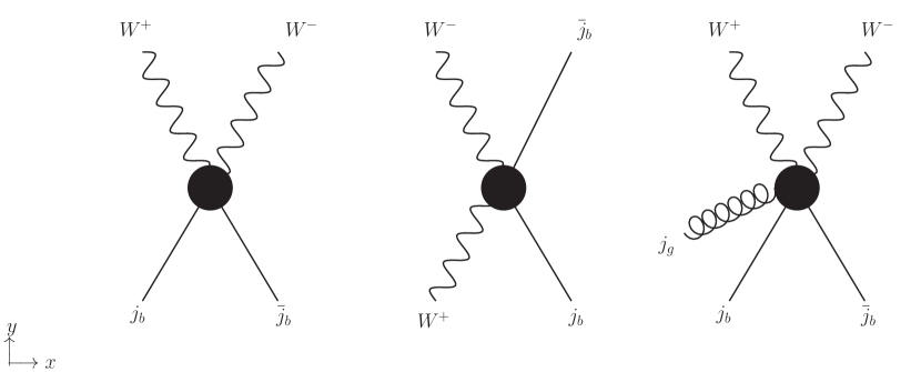
The options for $X_{B}$ are sensitive to different aspects of the $pp\to bW^{+}\bar{b}W^{-}+X$ kinematics, such as the relation between the $b$ quarks with the initial state, which, being colored, can influence the hadronization. For example, in Figure 2 we display two configurations (first and second event sketches) that can have similar total hardness, e.g., measured by $\left|p_{T,j_{b}}\right|+\left|p_{T,{j}_{\bar{b}}}\right|$, but might have considerably different $m_{j_{b}j_{\bar{b}}}$. For small $m_{j_{b}j_{\bar{b}}}$, the two $b$ quarks will tend to be more collinear, hence they have a greater chance to interfere with each other when hadronizing. On the other hand, the first and third event sketches might have similar $\left|p_{T,j_{b}}\right|+\left|p_{T,{j}_{\bar{b}}}\right|$ and $m_{j_{b}j_{\bar{b}}}$, but the hadronization may still differ because of the different center-of-mass energy, which is larger in the third type of events. The notion of center-of-mass energy of the initial partons in presence of invisible particles can be captured by the variable $\sqrt{s_{\text{min}}}$ proposed in [68], which would be a discriminant between the third and the first type of event.

Figure 2: Spacial representation of three kinematic configurations of the $W$ bosons and jets in the transverse plane. The three configurations depicted can be distinguished looking at several $\chi_{B}(X)$ variables. The first two can have the same $\left|p_{T,j_{b}}\right|+\left|p_{T,{j}_{\bar{b}}}\right|$, but different $m_{j_{b}j_{\bar{b}}}$, whereas the first and the third differ for $\sqrt{s_{\min}}$, despite having the same $m_{j_{b}j_{\bar{b}}}$ and $\left|p_{T,j_{b}}\right|+\left|p_{T,{j}_{\bar{b}}}\right|$.

In addition, if one wishes to probe the whole kinematic phase-space of the $b\bar{b}$ system and its hadrons, one can think of further observables. For a probe of emissions from the $b$ quarks we can use the relative azimuthal angle $\Delta\phi(j_{b}j_{\bar{b}})$, that is affected by $b\to bg$ splittings, hence it can be meaningful to constrain parton shower parameters. A similar angular observable for $B$-hadrons $\Delta\phi(B\bar{B})$ can also be employed thanks to its sensitivity to the angular features of the transition of quark into hadrons. Attempting to isolate the fragmentation effect of these angular observables, in the following we will also consider the difference between hadron and jet angular separation, that is $|\Delta\phi(j_{b}j_{\bar{b}})-\Delta\phi(B\bar{B})|$. Besides employing the azimuth $\phi$, we use the complementary information of polar angles in the distributions of $\Delta R(j_{b}j_{\bar{b}})$, $\Delta R(B\bar{B})$, and $|\Delta R(j_{b}j_{\bar{b}})-\Delta R(B\bar{B})|$. Moreover, we consider, as possible candidate calibration observables, the mass of the $b$-jet, $m_{j_{b}}$, which might help to constrain the shower parameters, and the ratio of the invariant mass of two $B$-hadrons over the mass of the two jets, namely $m_{B\bar{B}}/m_{j_{b}j_{\bar{b}}}$.

A caution must be taken: some of the observables might suffer from experimental effects that hinder the use of their precise measurement for a calibration. For instance, the $b$-jet mass or the $X_{B}$ variables used to normalize $\chi_{B}$ are, in principle, sensitive to jet energy scale uncertainties, which may spoil the accuracy on the calibration observables. We shall therefore consider two scenarios for the achievable precision on the calibration observables: an optimistic scenario in which the jet energy scale uncertainties do not inflate the total uncertainty, and another one where the accuracy is limited by these uncertainties at around 1%.

As a further exploration, we also study variables where jets are avoided altogether. One of them is the jet radial energy density $\rho(r)$ defined above, which needs jets only to identify the hadrons that enter the calculation. In addition we also consider other observables such as the ratios:

• $\frac{E_{B}}{E_{\ell}}$

• $\frac{E_{B}}{E_{\ell}+E_{\bar{\ell}}}$,

in which we use the lepton energy to make a dimensionless quantity of the energy out of a $B$-hadron. For these variables there is no use of jets so that a measurement with systematic uncertainties far below the percent level is achievable.

3.2.1 Variants of the calibration observables

Due to the complexity of the $t\bar{t}$ decay final state, it is possible to conceive variants of the above defined $\chi_{B}$. For instance, the inclusion of leptons in the “visible” system used for the computation of $\sqrt{s_{\text{min}}}$ is somewhat arbitrary. Furthermore, if the calibration observables were to be studied in a high-$p_{T}$ sample of $pp\to b\bar{b}$ events, there would be no leptons at all so that a comparison of resulting outputs to $t\bar{t}$ results would not be straightforward. Therefore, in addition to the standard definition of $\sqrt{s_{\text{min}}}$ in Ref. [68], which is written in terms of the “visible” transverse momentum

$$\sqrt{s_{\text{min}}}(M_{\text{inv}})=\sqrt{E_{\text{vis}}{}^{2}-P_{\text{z,vis}}^{2}}+\sqrt{\text{mET}^{2}+(\Sigma_{\text{inv}}M_{\text{inv}})^{2}}\,,$$ (5)

where $M_{\text{inv}}$ are hypothetical masses of invisible particles, we also employ a modified version in which the corresponding quantity is computed as if the charged leptons were invisible, hence part of the mET. We denote this definition as $\sqrt{s_{\text{min,}b\bar{b}}}$, where $E_{\text{vis}}$ and $P_{z,\text{vis}}$ are expressed in terms of the $b\bar{b}$ system only. Although $M_{\text{inv}}$ can carry whatever values, in the case of $\sqrt{s_{\min}}$, the masses of the invisible particles are simply set to be the same as the neutrino masses for LHC purposes. By contrast, in the case that the whole $W$ boson is regarded as invisible, one may conceive to use the physical $W$-boson mass for $M_{\text{inv}}$ in eq. (5). We have explicitly checked the effect of not taking the physical mass of the $W$ boson on our results and observed little dependence on this arbitrariness; therefore, throughout our analysis, we shall put $M_{\text{inv}}=0$ for $\sqrt{s_{\text{min,}b\bar{b}}}$.

4 Results on the calibration observables

For a simple but effective characterization of the impact of the Monte Carlo parameters, we start by computing the average values of the calibration-observable spectra, also referred in the following as the first Mellin moment, i.e., $\mathcal{M}^{(\mathcal{O})}_{1}$. The general expression of the $k$-th Mellin moment of a distribution with counts $\mathcal{O}_{j}$ and bins centered in $b_{j}$ reads:

$$\mathcal{M}^{(\mathcal{O})}_{k}=\sum_{j}b_{j}\mathcal{O}_{j}^{k}\,$$ (6)

Note that $k$ is not necessarily an integer. Since we will deal with only the first moment in our study, we name it with a simpler notation $\mathcal{M}_{\mathcal{O}}$. The spectra of the calibration observables and all our results in the following sections are obtained with samples obeying the following cuts on final-state jets and leptons:

$$p_{T,j}>30\leavevmode\nobreak\ \textrm{GeV},|\eta_{j}|<2.4\,,\quad p_{T,\ell}>20\leavevmode\nobreak\ \textrm{GeV},|\eta_{\ell}|<2.4\,.$$ (7)

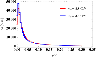
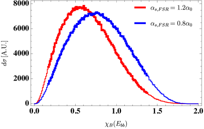
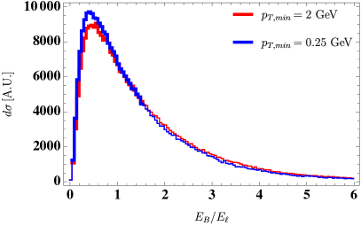
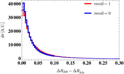
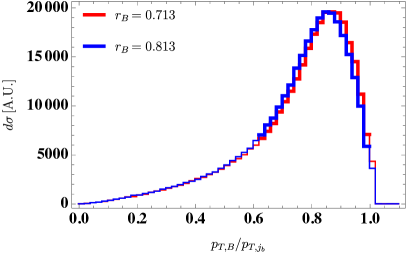
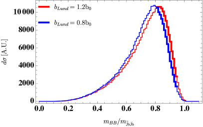
In order to avoid sensitivities to extreme kinematic configurations and the unknown unknowns about their theory description, we compute the average values in a range around the peak of the spectra. This range usually corresponds to the full width at half-maximum (FWHM) range, but in some cases we shall employ slightly different choices. For each observable we fix this range from the distribution that we obtain for one value of $m_{t}$, and we use it throughout the analysis. Our choices for the observables are reported in Table 4. Example spectra in observables that are potentially interesting for the calibration of the Monte Carlo parameters are shown in Figure 3, in which the thick part of the histograms corresponds to the FWHM range.

Figure 3: Example spectra for $\rho(r)$, $\chi_{B}(E_{j_{b}}+E_{\bar{j}_{b}})$, $E_{B}/E_{\ell}$, $\Delta R(BB)-\Delta R(j_{\bar{b}}j_{b})$, $p_{T,B}/p_{T,j_{b}}$, and $m_{B\bar{B}}/m_{j_{b}\bar{j}_{b}}$ for $m_{t}=174$ GeV.

4.1 Dependence on the top-quark mass

A preliminary step for the Monte Carlo tuning is the assessment of the dependence of the calibration observables on the top-quark mass. Ideally, a calibration observable should have no dependence on $m_{t}$, so that it could be used to constrain the Monte Carlo parameters without any concern about a potential bias in the $m_{t}$ measurement. In practice, all quantities have some sensitivity to $m_{t}$, so the only viable approach is using observables with minimal sensitivities to the top-quark mass. In this section we study the dependence on $m_{t}$ of the calibration observables, so that one can restrict the analysis to a specific set of quantities, clearly aimed at calibration.

We determine the dependence on $m_{t}$ of the first Mellin moments, obtained from 21 $m_{t}$ values in-between 163 GeV and 183 GeV, by fitting a straight line. We then compute the sensitivities defined in eq. (2) and repeat this procedure for the several Monte Carlo settings needed to explore the dependence on the parameters in Table 1. The Mellin moments and the straight-line fits for some illustrative parametrizations are presented in Figure 4. Once we have collected the values of the sensitivity to $m_{t}$ for all the variations of the Monte Carlo parameters, we calculate the mean value and standard deviation for each observable. We highlight the fact that the standard deviation, arising from the discrepancies in the straight-line fits to data with different parametrizations, is to be read as a measure of the sensitivity of our result to the Monte Carlo setting employed in the computation.

The results are reported in Table 4; a few comments are in order. First of all we remark that for our purposes it is sufficient to present the broad picture of the sensitivity of the observables to showering and hadronization parameters, and therefore we can content ourself with one or two digits of accuracy in the determination of sensitivity parameters. This accuracy will be more than sufficient to draw informative conclusions. Concerning the actual values of the sensitivity, we see that they tend to be $\Delta_{m_{t}}^{(\mathcal{M_{O}})}\ll 1$ for most observables, with few notable exceptions, the most apparent being the jet mass, which has $\Delta_{m_{t}}^{(\mathcal{M_{O}})}\simeq 0.23$. This is the only observable not constructed to be dimensionless, hence it is not surprising that it exhibits the largest sensitivity to the dimensional $m_{t}$. The smallest dependence on $m_{t}$ is found for the purely angular distributions $\Delta\phi(B\bar{B})$ and $\Delta\phi(j_{b}j_{\bar{b}})$, as well as their $\Delta R$ equivalents. In addition, we remark that the sample of variables $\chi_{B}$ tends to have slightly larger sensitivity to $m_{t}$. The choice of different denominators in $\chi_{B}$ can lead to a milder dependence on $m_{t}$ in the numerator, as can be seen by comparing the results for $\chi_{B}\left(\left|p_{T,j_{b}}\right|+\left|p_{T,\bar{j}_{b}}\right|\right)$ with respect to $\chi_{B}\left(E_{j_{b}}+E_{\bar{j}_{b}}\right)$.

4.2 Constraining power of the calibration observables

$\mathcal{O}$	Range	$\Delta_{m_{t}}^{(\mathcal{M_{O}})}$	$\Delta_{\theta}^{(\mathcal{M_{O}})}$
			$\alpha_{s,FSR}$	$m_{b}$	$p_{T,\text{min}}$	$a$	$b$	$r_{B}$	recoil
$\rho(r)$	0-0.04	-0.007(7)	0.78(1)	0.204(4)	-0.1286(8)	0.029(3)	-0.043(4)	0.056(7)	0.020(1)
$p_{T,B}/p_{T,j_{b}}$	0.6-0.998	-0.053(1)	-0.220(3)	-0.1397(8)	0.0353(5)	-0.0187(4)	0.0451(6)	-0.0518(9)	-0.0108(3)
$E_{B}/E_{j_{b}}$	0.6-0.998	-0.049(1)	-0.220(3)	-0.1381(8)	0.0360(5)	-0.0186(4)	0.0447(6)	-0.052(1)	-0.0107(3)
$E_{B}/E_{\ell}$	0.05-1.5	-0.155(7)	-0.156(3)	-0.053(3)	0.0149(7)	-0.007(2)	0.016(2)	-0.016(10)	-0.0087(7)
$E_{B}/(E_{\ell}+E_{\bar{\ell}})$	0.05-1.0	0.021(5)	-0.231(2)	-0.082(4)	0.0228(4)	-0.011(2)	0.026(2)	-0.028(6)	-0.0113(3)
$m(j_{\bar{b}})$/GeV	8-20	0.229(3)	0.218(1)	0.022(1)	-0.0219(7)	0.000(1)	-0.001(1)	0.001(3)	0.0050(3)
$\chi_{B}(\sqrt{s_{\text{min},bb}})$	0.075-0.875	-0.177(4)	-0.262(4)	-0.086(1)	0.0255(3)	-0.0105(10)	0.027(1)	-0.031(3)	-0.0137(2)
$\chi_{B}\left(E_{j_{b}}+E_{\bar{j}_{b}}\right)$	0.175-1.375	-0.109(2)	-0.357(4)	-0.134(1)	0.0373(3)	-0.016(1)	0.040(1)	-0.045(4)	-0.0175(3)
$\chi_{B}(m_{j_{b}j_{\bar{b}}})$	0.175-1.375	-0.089(3)	-0.252(3)	-0.080(1)	0.0248(3)	-0.010(1)	0.024(1)	-0.028(5)	-0.0126(2)
$\chi_{B}\left(\left|p_{T,j_{b}}\right|+\left|p_{T,\bar{j}_{b}}\right|\right)$	0.46-1.38	-0.15(2)	-0.47(1)	-0.189(10)	0.054(3)	-0.023(10)	0.06(1)	-0.07(4)	-0.022(2)
$m_{BB}/m{}_{j_{b}j_{\bar{b}}}$	0.8-0.95	-0.0191(8)	-0.0623(7)	-0.0464(5)	0.0146(2)	-0.0093(3)	0.0180(4)	-0.0212(9)	-0.00296(10)
$\Delta\phi(j_{b}j_{\bar{b}})$	0.28-3.	-0.210(7)	0.027(3)	0.001(2)	-0.0014(5)	-0.000(3)	-0.000(1)	-0.003(9)	0.0003(5)
$\Delta R(j_{b}j_{\bar{b}})$	1.4-3.3	-0.071(3)	0.010(1)	0.0005(10)	-0.0004(2)	-0.000(1)	0.0004(9)	0.001(3)	0.0001(2)
$\Delta\phi(BB)$	0.28-3.	-0.207(7)	0.026(2)	0.001(1)	-0.0008(4)	0.000(4)	0.000(2)	-0.000(8)	0.0002(5)
$\Delta R(BB)$	1.4-3.3	-0.070(3)	0.009(1)	0.000(1)	-0.0003(2)	-0.0003(10)	0.0002(9)	-0.000(4)	0.0001(2)
$|\Delta\phi(BB)-\Delta\phi(j_{b}j_{\bar{b}})|$	0-0.0488	0.06(1)	0.734(6)	0.099(5)	-0.088(2)	0.006(5)	-0.004(5)	0.01(2)	0.026(2)
$|\Delta R(BB)-\Delta R(j_{b}j_{\bar{b}})|$	0-0.0992	0.10(1)	0.920(3)	0.079(5)	-0.075(1)	-0.000(4)	0.005(4)	-0.00(2)	0.0418(8)

Table 4: Sensitivity of the calibration observables to the top quark mass and to the parameters of PYTHIA parton shower and hadronization. The quantities $\Delta_{m_{t}}^{(\mathcal{M_{O}})}$ and $\Delta_{\theta}^{(\mathcal{M_{O}})}$ are defined in the text. $\theta=\{\alpha_{s,FSR},\,m_{b},\,p_{T,\text{min}},\,a,\,b,\,r_{B},\,recoil\}$ denotes a generic PYTHIA parameter.

In order to quantify the dependence of the first Mellin moments on the Monte Carlo tuning, we evaluate the difference between the moments obtained for two values of each parameter at fixed $m_{t}$ and compute the sensitivity according to eq. (2) for the $m_{t}$ value at hand. Considering several $m_{t}$ values between 163 GeV and 183 GeV, we calculate the average value and standard deviation for the sensitivity $\Delta^{(\mathcal{M_{O}})}_{\theta}$ to each PYTHIA parameter in Table 4. The obtained estimate for the sensitivity essentially represents the distance between the lines shown in Figure 4 for different values of the same Monte Carlo parameter.

Figure 4: Dependence on $m_{t}$ of the average values $\langle\chi_{B}(E_{B}+E_{B})\rangle$ and $\langle m_{B\bar{B}}/m_{j_{b}\bar{j}_{b}}\rangle$. The error bars are due to the limited statistics of our calculation; the straight lines through the points are the fits employed to compute $\Delta_{m_{t}}^{(\mathcal{M}_{\mathcal{O}})}$.

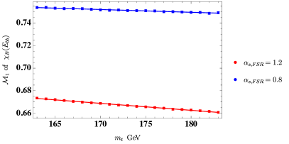
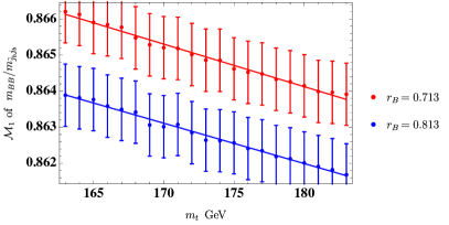
From Table 4, we can derive what precision in the measurement of the Mellin moments $\delta\mathcal{M}_{\mathcal{O}}/\mathcal{M}_{\mathcal{O}}$ should be reached to notice a given variation $\delta\theta/\theta$ of the Monte Carlo parameter. From the definition of the logarithmic derivative eq. (2) that we have tabulated, it follows:

$$\frac{\delta\mathcal{M}_{\mathcal{O}}}{\mathcal{M}_{\mathcal{O}}}=\Delta_{\theta}^{(\mathcal{M}_{\mathcal{O}})}\frac{\delta\theta}{\theta},$$ (8)

hence, observables with large $\Delta_{\theta}^{(\mathcal{M}_{\mathcal{O}})}$, are the best diagnostics of the accuracy of the tuning or, equivalently, the best observables for an in-situ calibration in the $t\bar{t}$ environment.

From a quick glance to the table, we find that a few interesting patterns emerge: the radial energy distribution $\rho(r)$ is among the most sensitive observables to both hadronization and shower parameters and tends to have opposite-sign sensitivity with respect to the other quantities. This tendency can be easily justified: for instance, when increasing $\alpha_{S,FSR}$, it is natural to expect more radiation, even at larger angles, so that $\langle\rho(r)\rangle$ grows, while $p_{T,B}$ or any possible denominator of $\chi_{B}$ decreases; a similar but reversed argument holds for $p_{T,\text{min}}$. In spite of this apparently different dependence of $\rho(r)$, we warn the readers that the actual usefulness of the combination of several observables to obtain constraints from data on the parameters has to be evaluated globally, by looking at the dependence of all observables on all parameters. We defer to Section 4.3 a full commentary on the information that we can obtain on the Monte Carlo parameters combining several calibration observables.

Angular variables like $\Delta\phi(B\bar{B})$ and $\Delta R$, as well as their analogs at $b$-jet level, tend to exhibit very small dependence on all parameters. However, the difference between hadron- and jet-level observables exhibits significant dependence on most parameters, as well as some similarity with the results for $\rho(r)$.

The hadron-to-jet ratios $p_{T,B}/p_{T,j_{b}}$, $E_{B}/E_{j_{b}}$, and $m_{B\bar{B}}/m_{j_{b}j_{\bar{b}}}$ exhibit substantial sensitivity to the Monte Carlo parameters and are expected to probe similar aspects of the PYTHIA description of the events. Due to the little dependence of $\Delta\phi$ and $\Delta R$ on both $m_{t}$ and shower/hadronization parameters, we can expect the sensitivity of the mass ratio to be closely related to that of the transverse-momentum ratio.

The ratios that involve lepton energies usually show very little sensitivity to the Monte Carlo parameters and $m_{t}$, and therefore they have little use for the calibration.

The variables $\chi_{B}$ show some of the largest sensitivity to the Monte Carlo parameters. We remark that for the denominator of $\chi_{B}$, the variants most sensitive to Monte Carlo parameters are those mostly dependent on $m_{t}$ as well. Usually, the increase of the dependence on the Monte Carlo parameters is smaller than the one on $m_{t}$. Nevertheless, care must be taken when one uses the definitions of $\chi_{B}$ more sensitive to $m_{t}$ in the calibration and in the $m_{t}$ determination.

The jet mass tends to have small dependence on the parameters, at most comparable to that exhibited by other observables. Putting this together with its large sensitivity to $m_{t}$, it is clearly a non-optimal candidate for a tuning or a measurement of $m_{t}$ with an in-situ Monte Carlo calibration.

4.3 Combined constraining power

In order to go beyond the qualitative analysis of the preceding paragraphs, we have devised a procedure, based on the $\Delta_{\theta}^{(\mathcal{M}_{\mathcal{O}})}$ values, to quantify the constraints on the Monte Carlo parameters which can be obtained from the combined use of several calibration observables. This procedure returns an estimate of the relative error on the determination of the parameters from the first Mellin moments, but can be straightforwardly applicable as well to other input observable quantities such as the higher Mellin moments or other properties of the spectrum of the calibration observables. The procedure goes as follows. We denote our parameters generically as a vector $\theta$, and collectively, we adopt the following notation:

$$\theta=\{\alpha_{s,FSR},\,m_{b},\,p_{T,\text{min}},\,a,\,b,\,r_{B},\,recoil\}\,.$$

We put the observables as well in a vector that we denote as $O=\{{\mathcal{O}_{i}}\}$ for the $\mathcal{O}_{i}$ listed in the first column of Table 4. In this notation the sensitivity of each observable to the several parameters can be expressed in matrix notation as:

$$\frac{\delta\mathcal{M_{O}}_{i}}{\mathcal{M_{O}}_{i}}=\left(\Delta_{\theta}^{(\mathcal{M_{O}})}\right)_{ij}\frac{\delta\theta_{j}}{\theta_{j}},$$ (9)

where Table 4 gives the entries $\left(\Delta_{\theta}^{(\mathcal{M_{O}})}\right)_{ij}$. This matrix contains all the necessary information to estimate how strong a constraint on the parameters $\theta$ can be obtained from measurements of the observables and their Mellin moments. In order to derive the constraining power of our set of calibration observables, we would like to invert the matrix $\Delta_{m_{t}}^{(\mathcal{M}_{\mathcal{O}})}$, as to express the sensitivity of the parameters as functions of the observables, which would take the relation of

$$\frac{\delta\theta_{j}}{\theta_{j}}=\left(\tilde{\Delta}_{\theta}^{(\mathcal{M_{O}})}\right)_{ij}\frac{\delta\mathcal{M_{O}}_{i}}{\mathcal{M_{O}}_{i}}\,,$$ (10)

with $\tilde{\Delta}_{\theta}^{(\mathcal{M_{O}})}$ satisfying

$$\tilde{\Delta}_{\theta}^{(\mathcal{M_{O}})}\cdot\Delta_{m_{t}}^{(\mathcal{M}_{\mathcal{O}})}=\mathds{1}\,.$$

Being aware that $\Delta_{m_{t}}^{(\mathcal{M}_{\mathcal{O}})}$ is, in general, a rectangular matrix, we may not be able to invert it to find $\tilde{\Delta}_{\theta}^{(\mathcal{M_{O}})}$. However, we can utilize the pseudo-inverse [69, 70] procedure to define $\tilde{\Delta}_{\theta}^{(\mathcal{M_{O}})}$: one defines linear combinations of observables and linear combinations of parameters such that each of the new observables depends only on one of the new parameters. To find these linear combinations, one can use a singular-value decomposition of the matrix $\Delta_{m_{t}}^{(\mathcal{M}_{\mathcal{O}})}$. The pseudo-inverse matrix is then the matrix obtained by acting on a diagonal matrix with values reciprocal to the singular values of $\Delta_{m_{t}}^{(\mathcal{M}_{\mathcal{O}})}$, with the inverse of the transformation that defines the new observables and new parameters. Further details on this procedure are given in Appendix A.

The strength of the constraints that can be obtained on the parameters $\theta$ is given by the general transformation of the covariance matrix. From eq. (10) it follows that

$$\mathbb{cov}_{\frac{d\theta}{\theta}}=\tilde{\Delta}_{\theta}^{(\mathcal{M_{O}})}\cdot\mathbb{cov}_{\frac{dO}{O}}\cdot\left.\tilde{\Delta}_{\theta}^{(\mathcal{M_{O}})}\right.^{t}\,.$$ (11)

Assuming for simplicity that the measurements of the Mellin moments are all uncorrelated and that an overall precision of 1% in their measurement is achievable, we find that the constraining power implied by Table 4 would be in general very modest. In fact, the standard deviations read off the diagonal elements of $\mathbb{cov}_{\frac{d\theta}{\theta}}$ are all around or above 100% relative uncertainty. The origin of this fact can easily be tracked back to the fact that the matrix $\Delta_{m_{t}}^{(\mathcal{M}_{\mathcal{O}})}$ has several small singular values: for Table 4 the singular values read 1.7, 0.26, 0.048, 0.0075, 0.005, 0.0033, 0.0014. This means that the information contained in the FWHM Mellin moments of the several observables which we consider allows us to constrain at most one or maybe two parameters (that would be $\alpha_{s,FSR}$ and $m_{b}$). In fact a singular value of order one means that from a measurement of the observables with precision 1% we can extract one parameter (or combination of Monte Carlo parameters) with the same accuracy, that is 1%. Similarly a singular value of order $10^{-3}$ implies that even in presence of a measurement of the observables with $10^{-4}$ precision we would obtain a constrain on the relevant (combination of) Monte Carlo parameters at a mere $10^{-1}$ level, as suggested by eq. (8). Given the singular values obtained, we remark that, even imagining measurements of the calibration observables with precision better than 1%, it is clear that an analysis of very inclusive quantities such as the Mellin moments is not capable of yielding any useful constraint on the Monte Carlo parameters.

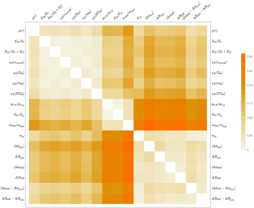
A more graphical way to picture why the Mellin moments do not contain enough information to constrain all the relevant Monte Carlo parameters is to look at the angles between the directions pointed by the rows of the matrix $\Delta_{m_{t}}^{(\mathcal{M}_{\mathcal{O}})}$. If two rows point in significantly different directions it means that two observables are sensitive to different combinations of the Monte Carlo parameters, hence their changes upon variations of the parameters are not much correlated. However, it turns out that for Table 4 all the rows point in a very similar direction. In Figure 5 we show the values of $1-|\cos\alpha_{ij}|$, where $\alpha_{ij}$ is the angle between the direction of the row $i$ and the row $j$. From the figure it is apparent that several Mellin moments point essentially in the same direction (e.g., $m_{BB}/m{}_{j_{b}j_{\bar{b}}}$, $p_{T,B}/p_{T,j_{b}}$, and $E_{B}/E_{j_{b}}$ are well visible in the center part of the plot); the two furthest apart directions are separated by $1-|\cos\alpha|\simeq 0.25$. Overall we can define three main directions which might be (somewhat arbitrarily) labeled by $\rho(r)$, for the observables in the upper left corner of Figure 5, $p_{T,B}/p_{T,j_{b}}$ for the observables in the middle part, and $|\Delta R(BB)-\Delta R(j_{b}j_{\bar{b}})|$ for the observables in the lower-right part.

Figure 5: Angular distance between the directions in parameter space pointed by the rows of Table 4.

Adding several higher Mellin moments to the analysis, we find very little change in the results of the analysis. We have tested values of $k$ in the definition of the $k$-th Mellin moment eq. (6) from 0.25 to 4 to explore the sensitivity of Mellin moments to the Monte Carlo parameters. We find that, although they have different magnitudes, all Mellin moments are sensitive to the same combinations of Monte Carlo parameters as in the first moment. We ascribe this similarity to the fact that we are considering FWHM ranges, which limits the possibility to be sensitive to different physical regimes, hence different Monte Carlo parameters. In the following section, seeking for an improvement of the prospected constraints, we explore the constraints that can be obtained if one considers the full range of the calibration observables.

4.4 Differential constraining power

More stringent constraints on the Monte Carlo parameters can be obtained exploring more in detail the full shape of the distribution of the calibration observables. A common practice in this case is to study several Mellin moments of the full distribution as a mean to probe the full shape of the observable at hand. However, in most cases one cannot extract the highest Mellin moments from the data very accurately, since they would be sensitive even to small errors in the distributions.

As an alternative, and probably more transparent, manner to study the shapes of the several observables, we use directly the bin counts of a subset of the calibration observables in suitably chosen ranges. The sensitivity of the bin counts to changes of the Monte Carlo parameters will be examined comparing bin-by-bin the spectra obtained from different Monte Carlo settings.

Figure 6: Differential sensitivity to the Monte Carlo parameters of the distributions of $p_{T,B}/p_{T,j_{b}}$, $m_{B\bar{B}}/m_{j_{b}\bar{j}_{b}}$, $\rho(r)$, and $\Delta R(BB)-\Delta R(j_{\bar{b}}j_{b})$. The two dashed vertical lines denote the FWHM ranges.

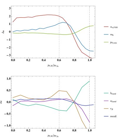
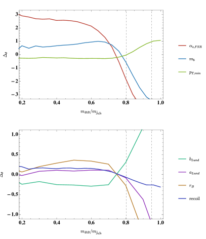
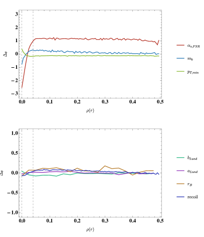
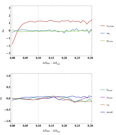
In order to keep the problem at a minimum of complexity, we start by identifying the most interesting physical quantities and studying the dependence of each bin count on the Monte Carlo parameters. Results for a few representative observables are presented in Figure 6, where the vertical dashed lines limit the FWHM ranges used in the previous section to compute the first Mellin moments of the distributions. These lines also serve as guidance to get a feeling of which parts of the distribution belong to the tails and which to the bulk. Clearly in some tails there is a good deal of sensitivity to the Monte Carlo parameters, but it is likely that data will be scarce in those regions.

From these results, we learn that sensitivities to $\alpha_{S,FSR}$ and $m_{b}$ exceeding 2 can be achieved, e.g., in $p_{T,B}/p_{T,j_{b}}$, whereas it is overall quite hard to find regions of the spectra with a similar dependence on $p_{T,min}$. The dependence on $a$, $b$, $r_{B}$ and $recoil$ is in general much milder.

Learning from the experience of the previous section, we can generalize the analysis by considering each bin as an independent observable and attempting to use its theoretical dependence on the Monte Carlo setting to constrain these. Similarly to the previous section, we can compute a matrix of sensitivity $\Delta_{\theta}^{(b_{j,\mathcal{O}})}$ with $(b_{j,\mathcal{O}})$ being the $j$-th bin of the distribution of the observable $\mathcal{O}$.

The observables that we use in this analysis are $\rho(r)$, $\chi_{B}(E_{j_{b}}+E_{\bar{j}_{b}})$, $E_{B}/E_{\ell}$, $\Delta R(B\bar{B})-\Delta R(j_{b}j_{\bar{b}})$, $p_{T,B}/p_{T,j_{b}}$, and $m_{B\bar{B}}/m_{j_{b}\bar{j}_{b}}$. They are the observables that in the previous section have shown the greatest sensitivity in absolute sense and the most distinct dependence on linearly independent combinations of Monte Carlo parameters. In place of the $\chi_{B}(E_{j_{b}}+E_{\bar{j}_{b}})$ variable we could have used other options for the denominator that appears in $\chi_{B}$, but we find it convenient employing $\chi_{B}(E_{j_{b}}+E_{\bar{j}_{b}})$, because it is bound to be in the range [0,2], facilitating the identification of an optimal bin-size for the calibration. This fact is quite important, because the study of distributions rather than integrated quantities inflates the expected statistical errors on the measurements. Using an observable that is limited to a range by definition (such as $\chi_{B}(E_{j_{b}}+E_{\bar{j_{b}}})$, $p_{T,B}/p_{T,j_{b}}$, and $m_{B\bar{B}}/m_{j_{b}\bar{j}_{b}}$), we can more easily define bins with sufficiently large expected number of events. In order not to deal with too small expected bin counts, we have divided each spectrum in about 10 bins, the details of the binning are reported in Table 5 for completeness.

$\mathcal{O}$	Range	$N_{bins}$
$\rho(r)$	0.-0.4	16
$p_{T,B}/p_{T,j_{b}}$	0.-0.99	11
$E_{B}/E_{\ell}$	0.05-4.55	9
$\chi_{B}\left(E_{j_{b}}+E_{\bar{j}_{b}}\right)$	0.-2.	10
$m_{BB}/m{}_{j_{b}j_{\bar{b}}}$	0.-0.998	11
$|\Delta R(BB)-\Delta R(j_{b}j_{\bar{b}})|$	0.-0.288	9

Table 5: Ranges and binning used for the calculation of the sensitivity of the bin counts of the full spectrum to changes of the Monte Carlo parameters.

We remark that by using a single observable and studying the whole spectrum the best results are obtained from the distribution of $p_{T,B}/p_{T,j_{b}}$. In this case the sensitivity matrix has singular values 7.0, 1.8, 0.28, 0.11, 0.11, 0.037, 0.018 from which we see a substantial improvement with respect to the case of Mellin moments in the FWHM range of the previous section. The largest angular distance in this case is $1-|\cos\alpha_{ij}|\simeq 0.45$, which clearly supports the observed sensitivity to more independent combinations of Monte Carlo parameters than in the inclusive analysis of Mellin moment. In spite of this, there are still several small singular values, which indicates that it is not possible to look only at this distribution to constrain all the parameters we set out to constrain. For completeness we report the sensitivity matrix for the $p_{T,B}/p_{T,j_{b}}$ distribution in Table 10 in Appendix A.

In order to obtain meaningful constraints on all Monte Carlo parameters of interest, it seems necessary to gather more information using a larger set of input observables. Performing such a global analysis on the six observables mentioned above, we find that the singular values of the sensitivity matrix are 15.0, 4.2, 0.75, 0.42, 0.27, 0.16, 0.13. Given the lowest singular value of order $10^{-1}$, we expect that it is possible to put meaningful bounds on all the parameters. For instance input observables measured at $10^{-2}$ precision should give $O(10^{-1})$ even on the most loosely constrained parameter.

We use eq. (11) to determine the covariance matrix expected for the determination of the Monte Carlo parameters from the study of the full spectrum of the six observables. If we assume that each bin of these distributions is an independent observable, uncorrelated with all the rest, and measured with 1% precision the expected relative uncertainty ranges from 70% for the recoil to about 4% for $\alpha_{s,FSR}$. Such uncertainties for all the parameters as well as the correlation matrix are given in Table 6. The reported uncertainties are for 1% precision on the input observables, treated as independent and uncorrelated. Had we considered a different precision for the input observables, for instance a 0.1% precision (reachable at the HL-LHC if one considers purely statistical uncertainties), we would have obtained linearly rescaled uncertainties (that is 10 times smaller than what are reported in Table 6), as eq. (11) dictates. These results clearly indicate that a global analysis of several spectra of calibration observables has a potential to constrain all the PYTHIA parameters explored here.

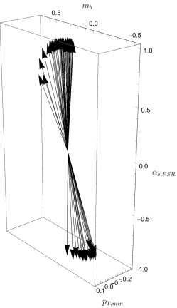
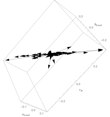
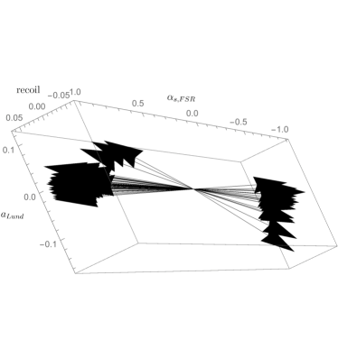
The improvement of the achievable constraint can be tracked to the angular distance between the rows of the sensitivity matrix that is larger than in the case of single observable analysis: for the six observables at hand we get $1-|\cos\alpha_{ij}|\lesssim 0.55$. Still, most of the information is extracted from bins in the distributions that depend on very similar combinations of the Monte Carlo parameters. This can be seen in Figure 7, where we display the direction of the gradient of the 66 bin counts used in our global analysis in various subspaces of our 7-dimensional parameter space. The shower parameters tend to appear in overall different combinations, although $p_{T,\textrm{min}}$ has usually small impact on the calibration observables, hence the gradient vectors in the top left panel have small components in the $p_{T,\textrm{min}}$ direction. The hadronization parameters, presented in the top right panel, tend to appear in combination $b-a-r_{B}$ except for a few observables, which generates the high degree of correlation in the matrix in Table 6. Finally in the bottom panel we find the dependence on the recoil switch parameter which shows significant correlation with $\alpha_{s,FSR}$.

We stress the fact that we have not gone through an intense optimization of the choice of the observables and ranges of the spectra, but nevertheless we expect these results to be illustrative of the achievable constraints on PYTHIA 8.

$\alpha_{s,FSR}$	$m_{b}$	$p_{T,\text{min}}$	$a$	$b$	$r_{B}$	recoil
0.045	0.14	0.35	0.5	0.48	0.21	0.73

$$\left(\begin{array}[]{ccccccc}1.&-0.13&0.48&-0.37&-0.24&0.38&-0.85\\ -0.13&1.&0.01&0.62&0.81&-0.46&-0.06\\ 0.48&0.01&1.&-0.09&-0.13&0.53&-0.08\\ -0.37&0.62&-0.09&1.&0.8&-0.47&0.31\\ -0.24&0.81&-0.13&0.8&1.&-0.23&0.15\\ 0.38&-0.46&0.53&-0.47&-0.23&1.&0.\\ -0.85&-0.06&-0.08&0.31&0.15&0.&1.\\ \end{array}\right)$$

Table 6: Top: expected relative uncertainties on the PYTHIA 8 parameters. assuming input observables measured with 1% accuracy. Bottom: correlation matrix for the constraint on these Monte Carlo parameters.

Figure 7: Directions in the $\{\alpha_{s,FSR},\,m_{b},\,p_{T,\text{min}}\}$ (top left), $\{a,\,b,\,r_{B}\}$ (top right) and $\{\alpha_{s,FSR},a,recoil\}$ (bottom) space pointed by the combination of parameters upon which the considered 66 bins of the distributions depend.

5 Results on observables sensitive to $m_{t}$

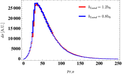
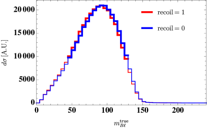
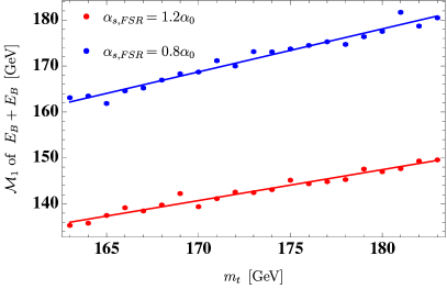
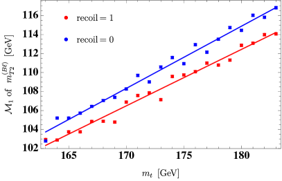
We are now in position to report our results on observables sensitive to $m_{t}$, following a similar path to the preceding section on calibration observables. We quantify the sensitivity of a mass-sensitive observable $\mathcal{O}$ to a given Monte Carlo parameter $\theta$ or to $m_{t}$, using a logarithmic derivative defined in eq. (2). The numerical derivatives necessary to compute $\Delta_{\theta}^{(m_{t})}$ are obtained from straight-line fits and comparison with Monte Carlo predictions varying the parameters in the same ranges as discussed for the purpose of the calibration variables. Examples of spectra for different Monte Carlo parameter settings are shown in Figure 8.

Figure 8: Example spectra of $p_{T,B}$, $E_{B}$, $E_{B}+E_{\bar{B}}$, $m_{B\ell}^{\textrm{true}}$, $m_{BB\ell\ell}$, and $E_{\ell^{+}}+E_{\ell^{-}}$ for $m_{t}=174\,\textrm{GeV}$.

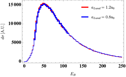
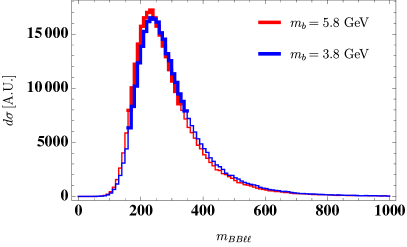
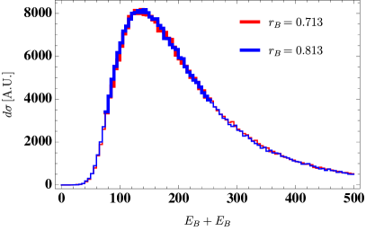
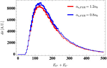
For mass-sensitive observables we would like to have a pattern of sensitivity that is opposite to the one wished for calibrations observables, that is to say large sensitivity to $m_{t}$ and small dependence on $\theta$. In fact, in order to reach a given accuracy $\delta m/m$ on $m_{t}$, we need to have under control each $\theta$ better than a relative precision

$$\frac{\delta\theta}{\theta}=\frac{\delta m}{m}\frac{1}{\Delta_{\theta}^{(m_{t})}}\,.$$

Therefore, the observables with smaller $\Delta_{\theta}^{(m_{t})}$ can be useful even when shower and hadronization parameters $\theta$ are not known well. As a consequence, for the observables to be used for the $m_{t}$ measurement we wish to have small $\Delta_{\theta}^{(m_{t})}$.

Due to possible different sensitivity to $m_{t}$ which different ranges of the distributions might exhibit, we will carry out two analyses. One is more inclusive and is based on the dependence of the Mellin moment of each observable on $m_{t}$ and the Monte Carlo parameters; the other one is based on the shape analysis of certain spectral features. These shape analyses are motivated by known properties of kinematic endpoints of distributions in e.g., $m_{B\ell}$ and $m_{T2}$, and of peaks of distributions in e.g., $E_{B}$, since the corresponding quantities constructed with a $b$-jet instead of a $B$-hadron are less affected by dynamical details. Hereafter, we shall first discuss the Mellin moments and then the shape investigation.

5.1 Mellin-moment observables

Similarly to the analysis carried out for the calibration observables in Section 4.2, we look at the first Mellin moment of the distributions of mass-sensitive observables, in order to characterize the dependence on $m_{t}$ and on the parameters $\theta$. We obtain each Mellin moment, restricting the calculation to a range that roughly corresponds to the Full-Width Half-Maximum area. The exact choices that we adopt in our analyses are reported in Table 7, together with the sensitivity values to each PYTHIA variables and to the top-quark mass. In the first rows of Table 7, we present results for observables that can be reconstructed with just one hadron, followed by those using also leptons. Then we present observables that would require the tagging of two $B$-hadrons and finally quantities that employ only leptons.

A further comment is in order concerning the numbers in Table 7. In the previous sections we have highlighted how a number of variations of some observables can be devised if we change strategy i) to pair together leptons and $B$-hadrons ii) to deal with the hadrons other than the $B$ in each jet iii) to deal with ISR, in the computation of $m_{B\ell}$ and $m_{T2}$. It turns out that the several variants of these observables tend to give rather similar results when it comes to both sensitivity to $m_{t}$ and to Monte Carlo parameters. For this reason we show only representative results for each type of observables. A similar table for HERWIG 6 parameters is given in Table 8, but it is limited to the most representative observables among those of the bigger set analyzed for PYTHIA.

Figure 9: Examples of $m_{t}$ dependence of the first Mellin moment of $p_{T,B}$, $E_{B}$, $E_{B}+E_{\bar{B}}$, $m_{B\ell}^{\textrm{true}}$, $m_{BB\ell\ell}$, and $m_{T2}^{(B\ell)}$ for different Monte Carlo parameters settings.

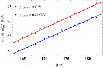
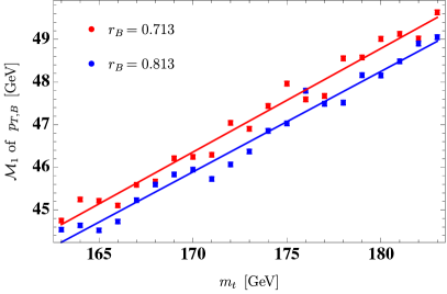
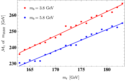
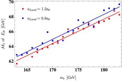
$\mathcal{O}$	Range	$\Delta_{m_{t}}^{(\mathcal{M}_{\mathcal{O}})}$	$\Delta_{\theta}^{(m_{t})}$
			$\alpha_{s,FSR}$	$m_{b}$	$p_{T,\text{min}}$	$a$	$b$	$r_{B}$	recoil
$E_{B}$	28-110	0.92(5)	-0.52(2)	-0.21(3)	0.057(4)	-0.02(2)	0.06(2)	-0.10(5)	-0.022(5)
$p_{T,B}$	24-72	0.92(3)	-0.54(2)	-0.21(2)	0.056(4)	-0.03(2)	0.07(1)	-0.09(4)	-0.023(2)
$m_{B\ell,\text{true}}$	47-125	1.30(2)	-0.241(8)	-0.072(6)	0.022(2)	-0.007(5)	0.023(6)	-0.02(2)	-0.008(2)
$m_{B\ell^{+},\text{min}}$	30-115	1.16(2)	-0.282(5)	-0.078(7)	0.024(2)	-0.011(7)	0.021(7)	-0.04(2)	-0.010(1)
$E_{B}+E_{B}$	83-244	0.92(4)	-0.50(2)	-0.21(2)	0.056(6)	-0.02(2)	0.07(3)	-0.08(6)	-0.020(4)
$m_{BB\ell\ell}$	172-329	0.96(2)	-0.25(1)	-0.10(1)	0.028(3)	-0.01(1)	0.026(7)	-0.03(3)	-0.008(2)
$m_{T2,B\ell,\text{true}}^{\text{(mET)}}$	73-148	0.95(3)	-0.27(1)	-0.09(1)	0.029(3)	-0.009(9)	0.03(1)	-0.03(4)	-0.010(3)
$m_{T2,B\ell,\text{min}}^{\text{(mET)}}$	73-148	0.95(3)	-0.27(1)	-0.09(1)	0.029(3)	-0.009(9)	0.03(1)	-0.03(4)	-0.010(3)
$m_{T2}^{(\ell\nu)}$	0.5-80	-0.118(7)	-0.03(2)	0.00(2)	0.002(8)	0.00(2)	-0.01(2)	0.00(7)	0.004(5)
$m_{\ell\ell}$	37.5-145	0.40(5)	-0.03(5)	-0.01(4)	0.00(1)	0.01(5)	0.01(4)	0.0(1)	0.00(1)
$E_{\ell}+E_{\ell}$	75-230	0.54(5)	-0.03(3)	0.00(3)	0.003(9)	0.01(3)	-0.00(2)	0.06(9)	0.003(8)
$E_{\ell}$	23-100	0.48(4)	-0.02(5)	0.00(5)	0.004(9)	0.01(4)	-0.01(4)	-0.06(9)	0.003(8)

Table 7: Columns under $\Delta_{\theta}^{(m_{t})}$ show the sensitivity to shower and hadronization PYTHIA parameters of the top quark mass extracted from the first Mellin moment of mass-sensitive observables. The column $\Delta_{m_{t}}^{(\mathcal{M}_{\mathcal{O}})}$ reports the sensitivity of the first Mellin moment to the top quark mass. The range extremal values reported in the second column are all in GeV. These ranges correspond to the FWHM for $m_{t}=174\textrm{GeV}$, for other masses we have used the corresponding FWHM.

$\mathcal{O}$	$\Delta_{m_{t}}^{(\mathcal{M}_{\mathcal{O}})}$	$\Delta_{\theta}^{(m_{t})}$
		PSPLT	QCDLAM	CLPOW	CLSMR(2)	CLMAX	RMASS(5)	RMASS(13)	VGCUT	VQCUT
$m_{B\ell,\text{true}}$	0.52	0.036(4)	-0.008(2)	-0.007(5)	0.002(3)	-0.007(4)	0.058(1)	0.06(5)	0.003(1)	-0.003(3)
$p_{T,B}$	0.47	0.072(1)	-0.03(9)	-0.02(7)	0.0035(5)	-0.03(5)	0.11(9)	0.12(5)	0.0066(2)	-0.006(5)
$E_{B}$	0.43	0.069(7)	-0.026(7)	-0.017(5)	0.0038(9)	-0.01(2)	0.12(1)	0.12(2)	0.006(2)	-0.007(5)
$E_{\ell}$	0.13	0.0005(5)	-0.04(3)	0.04(2)	-0.0002(2)	-0.004(4)	0.008(3)	0.008(2)	-0.002(5)	0.008(2)

Table 8: As in Table 7, but in terms of the HERWIG 6 shower and hadronization parameters. Ranges are those reported in Table 7 for all values of $m_{t}$.

Several interesting observations can be made on these tables. As for the PYTHIA study we find that the uncertainty on $\alpha_{S,FSR}$ has the largest impact on the $m_{t}$ measurement: a relative error on $\alpha_{s,FSR}$ around 1% seems necessary to achieve a 0.5%-level top quark mass determination. This level of precision in the knowledge of $\alpha_{s,FSR}$ is clearly signaling the overall necessity to describe radiation very accurately to attempt a precision measurement of the top quark mass. One could argue that the intrinsic error of a calculation based on a leading order matrix element attached to a leading-logarithmic parton shower, such as PYTHIA, makes it meaningless to talk about fixing one of its main parameters to such a precision. In fact, one can interpret our results as a starting point to conclude that $i$) a calculation with matrix elements computed beyond leading order matched to a parton shower might be used to (hopefully) get a smaller sensitivity to the $\alpha_{s,FSR}$ parameter and $ii$) a more accurate description of the parton shower beyond leading logarithms would probably be necessary as well to warrant a top-quark mass measurement from Monte Carlo simulations with sub-percent precision. In any case, for the scope of this paper, we will treat the findings on $\alpha_{s,FSR}$ at face value, hence we conclude that this parameter should be known with a precision from 1% to few %, for the sake of employing any observables which does not rely only on lepton momenta.

Concerning the other Monte Carlo variables, we observe that the $m_{t}$-dependent observables are much less sensitive to variations of the other parameters. The second most relevant one is the bottom-quark mass $m_{b}$, which, in order not to spoil the $m_{t}$ measurement, should be known with precision between few % and 10% from observables not made of just lepton momenta. Even smaller sensitivity values are obtained for $a$, $b$, $r_{B}$, $recoil$, and $p_{T,\text{min}}$: determining them to a 10% accuracy should be enough to warrant a 0.5% precision on $m_{t}$.

Purely hadronic quantities such as $p_{T,B}$, $E_{B}$, and $E_{B}+E_{\bar{B}}$ yield quite similar values of $\Delta^{(m_{t})}_{\theta}$. Therefore, the uncertainties due to hadronization and showering for a mass measurement based on any of these observables are expected to be essentially the same. Variables like $m_{B\ell}$ are in general half as sensitive as purely hadronic observables, hence they can tolerate a worse knowledge of the Monte Carlo parameters, even by a factor of 2. To better put these results in context, we can compare them to the sensitivity $\Delta^{(m_{t})}_{\theta}$ of other observables defined in terms of the charged leptons, such as the single-lepton energy $E_{\ell}$ and the invariant mass of the two leptons $m_{\ell\ell}$. In general, we observe a reduction by a factor of 10 or greater in $\Delta^{(m_{t})}_{\theta}$, in such a way that their parameter dependence in most cases becomes statistically compatible with zero. We can therefore argue that the mild sensitivity of observables like $m_{B\ell}$ is a genuine consequence of the small dependence of the lepton variables on the details of shower and hadronization.

As for HERWIG 6, our investigation is limited to the $B\ell$ “true” invariant mass, and the energy and transverse momentum of $B$-hadrons, and the energy of charged leptons in $W$ decay. For all observables and parameters, the $\Delta$ values run between values statistically compatible with zero and ${\cal O}(10^{-2})$, the highest dependence being exhibited by $m_{B\ell}$, $E_{B}$, and $p_{T,B}$ on $b$-quark and gluon effective masses, RMASS(5) and RMASS(13), and on the cluster-spectrum variable PSPLT(2). This implies that, aiming at a precision of 0.5% on $m_{t}$, it would be roughly sufficient to be aware of showering and hadronization parameters with about 10% accuracy. Before concluding this subsection, some comments on the tuning of the strong coupling constant are in order. Unlike PYTHIA, where different couplings for initial- and final-state radiation are employed and the value of the coupling at the $Z$ mass is possibly fitted, in HERWIG the user-defined quantity QCDLAM is a modified version of the $\overline{\rm MS}$ parameter $\Lambda_{\rm QCD}$, according to the CMW prescription [58]. It is easy to prove, using the formulas in [58] that a relative uncertainty of 10% on QCDLAM implies a precision about 1-2% on $\alpha_{S}(m_{Z})$ in the CMW scheme.

5.2 Shape Analyses

The Mellin-moment analysis above can be applied to all observables, since they all have a rise-and-fall shape and it appears reasonable to correlate it with $m_{t}$. However, for some observables, kinematic features such as peaks and endpoints are likely to yield more precise and more robust extractions of $m_{t}$ than the Mellin moments. These features might possibly protect one against uncertainties on showering and hadronization parameters. For example, at leading order and in the narrow-width approximation, the $m_{B\ell}$ endpoint arises from on-shell conditions of $W$ bosons and top quarks. For perfectly on-shell kinematics, regardless of the parton shower, such an endpoint should not be surpassed in any event, because it is completely dictated by the phase space of the top quark decay, and not by the underlying dynamics. Barring the soft colored quanta exchanged to neutralize the color of the top quark with the one of the rest of the event, the endpoint should be respected by all events, regardless of how the hadrons were formed. Motivated by this possible reduction of sensitivity to the Monte Carlo parameters, we extend our previous analysis to the kinematic endpoints of the $B\ell$ invariant mass and of the transverse mass $m_{T2}$ distributions, and to the peak position of the $B$-hadron energy spectrum. Endpoints and peaks will be determined by fitting their spectra with suitable functions.

5.2.1 Definition of the dedicated shape analyses

In order to extract the kinematic endpoints and energy-peak position, we analyze the part of the spectrum around them, employing fitting ansatze which capture the necessary features. For the kinematic endpoints, we take a simple second-order polynomial

$$y(x)=c_{1}(x-x_{m})^{2}+c_{2}(x-x_{m}),$$ (12)

where $x_{m}$ is identified as the corresponding endpoint and $c_{1,2}$ are other fit parameters, irrelevant to our study. For determining the peak position in a $B$-hadron spectrum, we adopt the following ansatz, inspired by the measurement of the $b$-jet energy peak in Ref. [71]:

$$y(x)\sim\exp\left[-p\left(\frac{x^{*}}{x}+\frac{x}{x^{*}}\right)\right]\,,$$ (13)

where $x^{*}$ is identified as the peak position and $p$ is another fitting parameter.

As for the endpoint of $m_{B\ell}$, we use the data in the range above $m_{B\ell}=127$ GeV, which corresponds to a fraction $\epsilon_{\text{tail}}\simeq 0.05$ of the total cross-section for $m_{B\ell,\text{true}}$ and $m_{t}=173$ GeV. In terms of the number of events $N_{ev}$ expected in each experiment at the LHC we have

$$N_{\text{ev}}\sim 5\times 10^{3}\cdot\frac{\mathcal{L}}{1\,\text{ab}^{-1}}\cdot\frac{\epsilon_{\text{tagging}}}{10^{-4}}\cdot\frac{\epsilon_{\text{tail}}}{0.05}\cdot{\rm BR}(t\bar{t})$$

where ${\rm BR}(t\bar{t})$ is the branching ratio of $t\bar{t}$ into a given decay mode, and $\epsilon_{\text{tagging}}$ is the tagging efficiency for an exclusive final state with a $B$-hadron. This estimate implies that the foreseen LHC dataset will yield statistical uncertainties ($\gtrsim 1.5\%$) somewhat above the level of the systematics at which we are aiming ($\sim 0.5\%$). There are several ways to get around the potential loss of overall precision due to the statistical uncertainty. First of all, if a tagging efficiency better than $10^{-4}$ could be achieved, for instance by not requiring exclusive $B$-hadron decays for tags, then the resulting statistical errors might become comparable to the systematic ones. Secondly, other experimental considerations may motivate to employ a broader range than the very end of the tail: for instance, in the CMS analysis [61] the $m_{b\ell}$ region used in the fit corresponds to $\epsilon_{\text{tail}}\sim 0.1$. One possible issue that one can raise with this trial is that the $m_{B\ell}$-endpoint analysis might indirectly reintroduce sensitivities to Monte Carlo parameters, through including more bulk of the distribution than endpoint region for the fit, resulting in an overall sensitivity to the Monte Carlo parameters similar to the Mellin moment analysis of the above Section 5.1. We have explicitly checked the sensitivities with smaller statistics, e.g., $\epsilon_{\text{tail}}\sim 0.02$, and found that there are no relevant effects. Nevertheless, we leave to the experimental collaborations the task of looking for an optimal balance; similar considerations, including the fit-range choice, apply to the other kinematic endpoints (see also Table 9).

For the study of the $E_{B}$-peak position it is much easier to secure enough statistics. Of course, the exact range of energies in which we analyze data affects the sensitivity to shower and hadronization parameters. In this case as well, we leave the optimal choice of range to the experimental collaborations. In our analysis, we simply take $[35,85]$ GeV for illustration, which corresponds roughly to the full width at three quarters of the maximum.

Finally, we make a further comment on notational conventions. Given the several options of reconstruction, subsystem and pairings, hereafter, for the sake of a more effective notation, the variants on which we focus will be labeled with roman letters in the math (min, true, ISR, mET). To avoid notational clutter with unnecessary indexes, we shall denote the endpoint of a mass distribution by a breve accent, i.e., $\breve{m}$, which should be evocative of our parabola fit near the endpoint.

5.2.2 Results of the dedicated shape analyses

The results on the sensitivity of our observables on the top-quark mass and of $m_{t}$ on the Monte Carlo parameters are reported in Table 9.

First of all we would like to comment on the form used to present these results: in fact, whenever the sensitivity of an observable to a given parameter is very small, it becomes numerically challenging to determine it. In the following we will be interested in identifying parameters that have remarkable effects on the observables; therefore, in presence of a small sensitivity, we will content ourselves with stating that it is below the few per-mil level, $\Delta_{\theta}^{(m_{t})}<0.003$. In fact, for an observable to be used to measure $m_{t}$, this level of sensitivity is clearly safe, as it implies that knowing just the order of magnitude of a given $\theta$ will be enough to warrant a $10^{-3}$ precision on $m_{t}$.

$\mathcal{O}$	Range	$\Delta_{m_{t}}^{(\mathcal{O})}$	$\Delta_{\theta}^{(m_{t})}$
			$\alpha_{s,FSR}$	$m_{b}$	$p_{T,\text{min}}$	$a$	$b$	$r_{B}$	recoil
$E_{B,\text{peak}}$	35-85	0.8(1)	-0.74(9)	-0.26(4)	0.05(1)	-0.04(2)	0.08(3)	-0.07(9)	-0.031(7)
$\breve{m}_{B\ell,\text{true}}$	127-150	1.26(1)	0.017(6)	0.003(9)	-0.006(2)	-0.008(2)	0.008(7)	-0.016(6)	-0.00042(9)
$\breve{m}_{B\ell,\text{min}}$	127-150	1.28(1)	-0.023(3)	-0.022(2)	0.006(3)	-0.008(3)	0.008(3)	-0.02(1)	-0.0001(6)
$\breve{m}_{T2,B\ell,\text{true}}^{\text{(mET)}}$	150-170	0.98(2)	-0.01(2)	-0.023(3)	0.007(1)	-0.006(3)	0.010(4)	-0.011(9)	-0.0002(8)
$\breve{m}_{T2,B\ell,\text{min}}^{\text{(mET)}}$	150-170	0.97(2)	-0.02(1)	-0.021(5)	0.006(2)	-0.006(3)	0.009(4)	-0.01(1)	-0.0001(8)
$\breve{m}_{T2,B\ell,\text{min,}\perp}^{\text{(mET)}}$	138-170	0.89(2)	-0.071(5)	-0.046(7)	0.012(2)	-0.011(7)	0.010(8)	-0.01(2)	-0.002(1)
$\breve{m}_{T2,B}^{\text{(mET)}}$	142-170	0.95(3)	-0.089(6)	-0.064(6)	0.018(1)	-0.017(4)	0.031(4)	-0.04(2)	-0.0028(8)
$\breve{m}_{T2,B,\perp}^{\text{(mET)}}$	126-170	0.94(4)	-0.07(1)	-0.04(1)	0.011(3)	-0.009(9)	0.02(1)	-0.03(4)	-0.001(2)

Table 9: Sensitivity to shower and hadronization parameters of the top quark mass extracted from a shape analysis of special feature in the spectra of $E_{B}$, $m_{B\ell}$, $m_{T2}$. The range extremal values reported in the second column are all in GeV.

For the energy-peak fit, we find results rather close to those from the Mellin-moment analysis: regarding hadronization and showering uncertainties, determinations of $m_{t}$ from a moment or from energy peaks are on the same footing. In fact, top-quark decays $t\to W^{+}B+{\rm hadrons}$ are genuinely multi-body processes, hence the $B$-energy peak does not fully enjoy the process-independent “invariance” property of the peak in $b$-jet energy spectra [71, 72], which, instead is typical for a two-body process such as $t\to j_{b}W^{+}$ with $j_{b}=B+\text{hadrons}$.

For the $B\ell$ invariant mass, the endpoint analysis shows a very significant reduction of shower and hadronization sensitivity: in fact, the upper-bound on $m_{B\ell}$ is roughly the same as for an ideal two-step two-body on-shell decay, i.e., $B\rightarrow b$ limit where no shower or hadronization effect comes into play. However, we remind that in practice the endpoint is extracted by fitting a certain amount of bulk region with a suitable template, e.g., a parabola in Eq. (12). As discussed before, the endpoint measurement is indirectly affected by the Monte Carlo parameters via fit parameters $c_{1}$ and $c_{2}$ in Eq. (12) that are responsible for the detailed shape near the endpoint. In the chosen range, the dependence of $m_{B\ell}$ on hadronization and showering parameters is milder by an order of magnitude with respect to the Mellin moment analysis. In some cases, the sensitivity is even below the statistical uncertainty: for example, the binary choice of the conservation of momentum in the shower, which has a $\Delta_{\text{recoil}}\sim 0.02$ in the $m_{B\ell}$ Mellin analysis, becomes completely negligible for the endpoint strategy. As for $p_{T,\text{min}}$, $a$, $b$, and $r_{B}$, the corresponding $\Delta_{\theta}^{(m_{t})}$ are ${\cal O}(10^{-3})$, hence they are borderline to be irrelevant; $\alpha_{S,FSR}$ and $m_{b}$ carry small impacts, although not completely negligible. It should be remarked that these results rely on using only portion of the spectrum in the parabola fit.

As for $m_{T2}$, all variants perform in a very similar way, with sensitivity being (mostly) as reasonably small as $\Delta\sim{\cal O}(10^{-3})$. Very little difference appears between the “min” and “true” options, and therefore, it seems that the pairing or combinatorial issue does not make a worrisome impact on the mass measurement. The mET and ISR prescriptions show a comparable dependence on the Monte Carlo parameters, for both $B$- and the $B\ell$-subsystems (see also Appendix B for a complete list). The mET ones exhibit the smaller sensitivity to some parameters, while the ISR ones are less dependent on other variables. Therefore, both prescriptions should be considered equally good to determine $m_{t}$. Again, these results hold for the analysis with relatively narrow fitting ranges towards the tails, yielding reliable parabola fits of the endpoints, even with no reference to the details of the reconstruction. As for $m_{T2}$ in the $B$-subsystem, given the little difference between the “min” and “true” cases in the $B\ell$-subsystem, the use of the $B$-subsystem options loses some of its initial motivations. However, it exhibits a dependence on the Monte Carlo parameters very close to the lowest of $m_{T2}$, hence it can be a useful validation of the $B\ell$ results.

One notable feature has to do with the “perp” correction applied to the variables denoted by the $\perp$ subscript. In this subsystem, the $\perp$-correction leads to a slight reduction of the sensitivity to the Monte Carlo parameters, in particular, to $\alpha_{S,FSR}$ and $m_{B}$ for the mET prescription. By performing the $\perp$-correction, any process-dependent effect in association with initial-state radiation, which is somehow convoluted with the Monte Carlo parameters of interest, is detached, so that the resulting sensitivity gets reduced. By contrast, such a reduction does not arise for the ISR-reconstruction scheme, since the $\perp$-correction itself carries over its own sensitivity to the parameters through $A+\bar{A}$. The $\perp$-variants in the $B\ell$ subsystem are somewhat more involved: Here the inclusion of leptons in constructing the variables already mitigates the sensitivity, even before applying the $\perp$-correction. It turns out that the net effect resulting from the $\perp$-correction is not friendly in the $B\ell$ subsystem. Nevertheless, this class of variables are worth investigating, in the sense of probing sensitivities to the Monte Carlo parameters with any production-dependent effects decoupled.

Overall, we find a conclusion similar to the Mellin analysis: ISR in $t\bar{t}$ production, pairing leptons and $B$-hadrons, as well as the treatment of light-flavored hadrons in the $b$-jet, are all largely orthogonal from the viewpoint of the sensitivity to the Monte Carlo hadronization parameters.

6 Conclusions

The accurate measurement of the top-quark mass is one of the major goals for the physics program of the Large Hadron Collider. The level of precision that is demanded for $m_{t}$ to be useful in the context of physics of the Standard Model and in tests of new physics is around 500 MeV, well below the percent level.

Carrying out a measurement at such a level of accuracy is challenging and has generated a number of proposals. All strategies rely to some extent on our ability to predict some observables by means of a QCD calculation or a Monte Carlo simulation, e.g., a total or fiducial rate of top quark production, or the shapes of some differential distributions: all such methods exhibit an associated theoretical error. Presently, most precise determinations of $m_{t}$ use quantities that are believed to be less affected by theoretical errors, such as the peak of invariant mass obtained with kinematic (template) methods, which essentially tries to capture the peak in $b$-jet$+W$ invariant mass in top-quark decay. In this case the most important systematic uncertainty is the jet energy scale, namely the correction necessary to measure the true jet energy from the measured detector response. These corrections have been the subject of intense studies and could be improved in future, but probably only modestly. Therefore, it seems that it may not be possible to improve significantly the measurement of the top-quark mass from these “standard” methods.

Motivated by the above drawbacks, a number of “alternative” strategies have been proposed and will acquire even more importance in the future. In fact, many of the alternative techniques pursue different strategies than the “standard” methods, and hence they will allow to cross-check the available and existing results, eventually giving rise to a global determination of $m_{t}$, accounting for measurements performed by using inherently different strategies. Of course, the most useful measurements in this combination will be those that are not affected significantly by the jet energy correction, which presently dominates the uncertainty on $m_{t}$. Among the proposals, there are measurements that utilize only leptons from semi-leptonic and di-leptonic final states of $t\bar{t}$ decays and others that employ exclusive and semi-exclusive hadronic final states. In both cases there is no reference to jets in the formulation of the observables that are used to extract $m_{t}$ from the comparison of data and calculations, and therefore the jet energy correction has a very minor effect in these measurements. These observables are, however, not free from uncertainties: in fact, when dealing with hadrons, one clearly encounters the difficulty to carry out theoretical predictions for such final states. For leptonic final states as well, there are residual theory errors because the distributions that one uses to extract $m_{t}$ are usually less sensitive to $m_{t}$, but they still carry some non-negligible sensitivity to the theoretical modeling, e.g., to missing orders in perturbation theory or to the description of the production mechanism of the top quarks at the LHC.

The goal of our work was to quantify the uncertainty on the top-quark mass extraction due to our limited ability to compute observables for exclusive hadronic final states. We have considered a number of possible observables that can be defined on exclusive hadronic final states, both drawing from the literature and introducing some new ones, potentially useful to explore the achievable precision on $m_{t}$ from the study of hadrons in $t\bar{t}$ samples. We have concentrated our efforts on Monte Carlo event generators and the dependence of the predictions on their tunable parameters. As discussed throughout the paper, Monte Carlo codes are often used to derive predictions on exclusive hadronic final states at colliders and are often preferred over theoretical approaches, such as resummed calculations in the fragmentation function formalism, which, as discussed in the Introduction, tend have a difficulty i) to give predictions for generic observables, that can instead be obtained from Monte Carlo programs; ii) to give precise-enough predictions at least by using the currently available perturbative computations, which are typically NLO+NLL, and iii) to yield results at hadron level without relying on phenomenological non-perturbative models, which are often too simple to describe the data and eventually meet the LHC precision goals. Therefore we believe that a study of exclusive hadronic final states is best carried out employing Monte Carlo event generators.

We have simulated $t\bar{t}$ events by means of the PYTHIA 8 and HERWIG 6 programs, which differ considerably in the description of both emissions of soft and collinear partons in the so-called “parton shower” and of the formation of hadrons. Looking at both approaches, we are able to evaluate the peculiarities of the codes and identify the common issues which are to be addressed in the top-quark mass measurement strategies.

For both codes, we have evaluated the dependence of several observables on $m_{t}$ and on the most relevant Monte Carlo parameters. To simplify the understanding of the results, we have introduced a sensitivity measure $\Delta$, defined in eq.(2), which allows to look in a uniform way to the vast number of results that we have collected in our tables. The sensitivity has been computed for the mean value of each quantity, calculated in a specific range, which corresponds approximately to the bulk of the distribution of the observable.

The observables belong roughly to the following classes: purely hadronic observables, e.g. the $p_{T}$ of the $B$-hadron, mixed leptonic-hadronic observables, e.g. the invariant mass $m_{B\ell}$, and purely leptonic observables, e.g. the lepton energy $E_{\ell}$. As could have been anticipated, the description of the hadronic final states is very important for purely hadronic observables and slightly less important for the mixed leptonic-hadronic ones. Leptonic quantities usually have so small dependence on the Monte Carlo parameters, that we observe a dependence compatible with zero within our statistical uncertainties arising from limited simulated data sample.

More quantitatively, we find that, in order to warrant a 0.5 GeV precision on the $m_{t}$ extraction from hadronic and mixed leptonic-hadronic observables, most parameters must be known with a precision around 10% in both PYTHIA and HERWIG: it is clear that such an accuracy cannot be attained without inputs from data. We will discuss shortly how the interplay between data, parameters and the measurement of the top quark mass might unfold. Before doing that, we highlight that for both PYTHIA and HERWIG it seems necessary to have an even more precise knowledge of the strong coupling constant used in the parton shower. For PYTHIA which uses a parameter named $\alpha_{s,FSR}$, corresponding to $\alpha_{s}(m_{Z})$ with a one-loop evolution, we find that hadronic and mixed leptonic-hadronic observables demand the knowledge of $\alpha_{s,FSR}$ with a precision from 1% up to a few %. The necessity to fix $\alpha_{s}$ so precisely clearly signals the need for improved theoretical predictions, which could be ultimately achieved by using beyond-LO hard matrix elements as well as a more accurate description of the parton shower, e.g., in the NLL approximation. In any case, even within our study with the present parton shower accuracy, the message is clear: the description of radiation is of utmost importance for the measurement of $m_{t}$ if one uses any observable that involves hadrons.

The striking precision with which it is necessary to know the Monte Carlo parameters motivated two further explorations in our analysis: i) the study of more robust observables, possibly less sensitive to the Monte Carlo parameters that necessarily act as nuisances in the $m_{t}$ determination; ii) the investigation of a strategy to derive directly from data the value of the Monte Carlo parameters to be used for the mass extraction.

For the former, we have studied the use of kinematic endpoints of certain masses that are known to carry information on the top quark mass. To this end, we investigated the endpoints of $m_{B\ell}$ and of several variants of the $m_{T2}$ variable which can be constructed from the four observable final state particles (i.e., two $B$ hadrons and two leptons) of the fully leptonic $t\bar{t}$ decay. A crucial observation drawn from our scrutiny is that studying the regions very close to the endpoint enables us to make predictions sufficiently independent from Monte Carlo parameters. The price to pay for this is to reduce the number of events to be analyzed, hence inflating the statistical uncertainties to a level jeopardizing the entire strategy. In other words, the resulting statistical uncertainty can be even beyond the level of theoretical uncertainty that we aim to achieve. Furthermore, it should be remarked that, when one concentrates on the region of the spectrum so close to the endpoint, the current limit in the Monte Carlo description, e.g., “off-shell” production of top quarks, not-calculated perturbative higher orders, which were assumed sub-dominant and hence neglected in our study, might start to play an important role. To alleviate this issue one would be forced to consider a larger portion of the spectrum, hence reintroducing a larger dependence on the Monte Carlo parameters. Seeking a balance between statistical and Monte Carlo uncertainties parameters will hence be a delicate task for the experimental collaborations.

Clearly, if one had a good knowledge of the Monte Carlo parameters, all the above-mentioned conclusions on the uncertainties in the top quark mass determination could be improved. For this reason we have studied what kind of constraints can be obtained from data if one tries to use a number of measured distributions in $t\bar{t}$ events in order to adjust the parameters in the Monte Carlo event generators. We have restricted a majority of our study to PYTHIA, expecting that the general conclusions and observations obtained with PYTHIA will be valid for HERWIG as well.

The effort of reproducing measured distributions varying the parameters might be considered as a “tuning” similar to the general-purpose tunings which exist for Monte Carlo generators. However, we remark that for the mass measurements outlined above it is necessary to “tune” $\alpha_{s}$ to about 1% precision and other parameters around 10% precision. Therefore, one should take this tuning in part as an attempt to capture physics effects that go beyond the approximation inherent in the use of the parton shower approach. In other words, in the fitting procedure, one incorporates in the parameters all the effects due to the incomplete description of perturbative and non-perturbative physics in the event generator. Therefore, our tuning is quite likely to be specific to the top-quark events, while in general it may not be valid for other processes. Therefore, even if PYTHIA is eventually tuned to top-quark data, it will be very unlikely for such fits to be “universal”, i.e., they are not expected to be reliable outside the very same data sample accounted for in the parameter adjustment. For this reason we would like better to call this procedure a “calibration” of the Monte Carlo variables, specific to $t\bar{t}$ processes. Such a calibration is ideally performed on the same data as what will be used to measure the top-quark mass, hence we might call this strategy a $m_{t}$ determination, in conjunction with an “in-situ” Monte Carlo calibration.

As for PYTHIA, we have studied seven parameters which affect the showering and hadronization modeling. We find that, in order to constrain them from $t\bar{t}$ data, one has to examine the detailed shape of several observables, as the study of more inclusive quantities (e.g., averages in a range) may not be enough. We further observe that it is necessary to carry out a global analysis with several quantities, as no single-observable exploration can constrain all the necessary parameters.

In summary, we find that using simple features, e.g., the mean of the spectra, to extract the top-quark mass requires good knowledge on the Monte Carlo parameters. Such parameters can be obtained from the very same data sample used to determine $m_{t}$, but looking at observables which have sufficiently large dependence on the parameters and very little sensitivity to $m_{t}$. This “in-situ” calibration of the Monte Carlo event generator might warrant a sufficiently small theoretical error to obtain $m_{t}$ from exclusive hadronic final states, but it may be necessary to carry out a detailed shape analysis of several observables at once. Despite correlations among the calibration quantities, it seems that the required precision can ultimately be achieved if one is able to measure the observable shapes with about 1% accuracy, which may be challenging. Furthermore, our results might be altered by experimental systematics and correlations among measurements that we have not evaluated (e.g., a correlation in the calibration observables due to common experimental systematics). For this reason, one might look at endpoints of some distributions which are known to be sensitive to the top quark mass, e.g., the endpoint of $m_{B\ell}$. For such observables, we have demonstrated that the effect of the Monte Carlo parameters can be suppressed at the cost of larger statistical uncertainties. It remains as a future work to pursue an optimal balance between endpoint analyses versus studies of the bulk of the distributions, in view of the performances that can be achieved through the “in-situ” Monte Carlo calibration.

The present work can also be extended along several lines. Although in the introduction we discussed the role that it plays in the uncertainty in the top-mass determination, color reconnection was not explored in our investigation. Nevertheless, studying the impact of color-reconnection models and parameters, along the lines of [48], on Mellin moments, peaks and endpoints of $B$-hadron observables is certainly mandatory for the sake of completeness. Furthermore, even if $t\bar{t}$-production processes are mostly high transverse-momentum events, investigating the effect on the top mass of the modeling of the underlying event and of the implementation of multiple scatterings is definitely compelling.

Regarding Monte Carlo generators, the HERWIG 6 code, which we used through our analysis, is outdated and not supported anymore. Therefore, it will be much useful updating our investigation by employing the latest object-oriented HERWIG 7.1 code. In fact, as debated in the introduction, its description of bottom-quark fragmentation is not optimal, but, thanks to the implementation of the new dipole-shower model and a number of novel features for the purpose of the treatment of heavy quarks, the comparison with $B$-hadron data at $e^{+}e^{-}$ machines has much improved with respect to previous versions [56]. Analyzing the dependence of calibration and $m_{t}$-dependent observables on the parameters of HERWIG 7.1 will hence be very instructive.

Finally, an obvious extension of our study consists of using NLO+shower codes, such as the latest version of aMC@NLO [12], SHERPA [18] and especially POWHEG [13], which accounts for NLO corrections to top decays, width and non-resonant effects. We plan to explore our $B$-hadron observables by using aMC@NLO, POWHEG and SHERPA, in order to check their sensitivity to non-perturbative parameters and whether it is different from the case of standard LO event generators. In fact, on the one hand, one should expect that, thanks to the improved description of the perturbative part of the $t\bar{t}$ event simulation, the dependence on non-perturbative parameters should become milder. On the other hand, however, a recent analysis on the determination of the top mass [73] using NLO+shower codes has displayed substantial discrepancies according to whether the latest POWHEG version is interfaced to HERWIG 7 or PYTHIA 8 for parton cascades, hadronization and underlying event. Exploring the parameter dependence of calibration and top-mass observables yielded by POWHEG interfaced to HERWIG 7 or PYTHIA 8 should possibly help to shed light on the discrepancy in the mass extraction pointed out in [73]. This is in progress as well.

Appendix A Determination of the sensitivity matrix

In the regime in which the observables are linear functions of the parameters

$$O_{i}=c_{i}+D_{ij}\theta_{j}$$

we define $\tilde{O}_{i}=O_{i}-c_{i}$, such that

$$\tilde{O}=D\theta$$ (14)

where $D$ is a $N_{O}\times N_{\theta}$ matrix. The matrix can be said to contain the derivatives of the observables w.r.t. the parameters

$$\frac{d\tilde{O}_{i}}{d\theta_{j}}=\frac{dO_{i}}{d\theta_{j}}=D_{ij}\,.$$

Since $d\tilde{O}=dO$ we will use them interchangeably at our convenience.

If we want to derive the parameters that correspond to a certain measurement of the observables, we should invert $D$, which may not be rigorously possible when $D$ is not a square matrix. In place of the inverse, we use its pseudo-inverse [69, 70], that we denote as $D^{-1}$, and which can be computed by a singular-value decomposition of $D$. The singular-value decomposition allows to write $D$ as the product of three matrices $D=\Omega^{-1}\hat{D}P$ which can be understood as a change of basis in the vector parameter space operated by $P$, a change of basis in the observable space operated by $\Omega$, and a matrix $\hat{D}$ which gives the linear dependence of the observables on the parameters in the new basis. The matrix $\hat{D}$ is diagonal, hence the matrix made of its reciprocal diagonal values can be used to define the pseudo-inverse in such a way that $\hat{D}D=\mathds{1}$. With this definition we can write

$$\theta=D^{-1}\tilde{O}=\left(P^{-1}\hat{D}^{-1}\Omega\right)\tilde{O}\,.$$

If we desire to work entirely with relative uncertainties, we can restart from eq. (14) and make a change of variables by rescaling the parameters and the observables by suitable factors that turn error propagation into an expression where only relative errors appear. We define $\bar{\theta}$ rescaling values so that each parameter is a dimensionless fudge-factor

$$f_{\theta_{i}}\equiv\frac{\theta_{i}}{\bar{\theta}_{i}}=\Lambda_{\theta}\theta=\left(\begin{array}[]{ccc}\frac{1}{\bar{\theta}_{1}}\\ &\ddots\\ &&\frac{1}{\bar{\theta}_{N}}\end{array}\right)_{ij}\theta_{j}$$

Using this redefinition in eq. (14) we get

$$\tilde{O}=D\theta=D\Lambda_{\theta}^{-1}\,f_{\theta_{i}}\,.$$

Similarly we can define a convenient value to rescale $\tilde{O}$ and make them dimensionless

$$f_{\tilde{O}_{i}}=\frac{\tilde{O}_{i}}{\bar{O}_{i}}=\left(\Lambda_{O}\tilde{O}\right)_{i},$$

so that eq. (14) now reads

$$\Lambda_{O}^{-1}f_{\tilde{O}}=D\Lambda_{\theta}^{-1}\,f_{\theta_{i}}\,$$

and ultimately

$$f_{\tilde{O}}=\Lambda_{O}D\Lambda_{\theta}^{-1}\,f_{\theta_{i}}\,.$$

The last line involves dimensionless fudge-factors $f$ and the sensitivity matrix $\Delta$ whose elements are

$$\Delta_{ij}\equiv\frac{d\tilde{O}_{i}}{d\theta_{j}}\frac{\bar{\theta_{j}}}{\bar{O_{i}}}=\frac{dO_{i}}{d\theta_{j}}\frac{\bar{\theta_{j}}}{\bar{O_{i}}}\,.$$

Once we know the linear mapping between the dimensionless fudge factors, we can use eq. (11) to find out the covariance matrix of one as a function of the covariance of the others.

As an example, Table 10 presents the sensitivity matrix for the $p_{T,B}/p_{T,j_{b}}$ ratio in terms of the PYTHIA parameters, in each bin.

$p_{T,B}/p_{T,j_{b}}$ range	$\alpha_{s,FSR}$	$m_{b}$	$p_{T,\text{min}}$	$a$	$b$	$r_{B}$	recoil
[0,0.09)	1.76(8)	0.12(10)	-0.05(4)	0.00(9)	-0.1(1)	-0.1(3)	0.09(2)
[0.09,0.18)	1.90(3)	0.12(3)	-0.08(1)	0.01(6)	-0.04(6)	-0.0(1)	0.094(9)
[0.18,0.27)	1.95(4)	0.18(4)	-0.095(6)	0.02(3)	-0.08(4)	0.1(1)	0.114(7)
[0.27,0.36)	2.06(3)	0.27(2)	-0.11(1)	0.01(3)	-0.07(3)	0.08(9)	0.128(8)
[0.36,0.45)	2.18(2)	0.40(2)	-0.141(4)	0.04(2)	-0.11(2)	0.15(7)	0.142(5)
[0.45,0.54)	2.26(1)	0.61(1)	-0.186(5)	0.04(2)	-0.16(1)	0.11(7)	0.155(4)
[0.54,0.63)	2.22(1)	0.90(1)	-0.246(4)	0.07(1)	-0.24(1)	0.27(4)	0.150(4)
[0.63,0.72)	1.81(1)	1.18(1)	-0.305(3)	0.11(1)	-0.36(1)	0.39(4)	0.121(3)
[0.72,0.81)	0.55(3)	0.78(2)	-0.256(2)	0.130(8)	-0.32(1)	0.38(3)	0.036(2)
[0.81,0.90)	-1.38(4)	-0.60(2)	0.015(3)	0.028(8)	0.08(1)	-0.06(2)	-0.063(3)
[0.90,0.99)	-2.65(5)	-1.82(2)	0.449(10)	-0.300(8)	0.656(7)	-0.77(2)	-0.133(4)

Table 10: Sensitivity of the bin counting of the $p_{T,B}/p_{T,j_{b}}$ distribution to variations of the PYTHIA 8 parameters.

Appendix B Sensitivities and special features of $m_{T2}$

For completeness, we report the sensitivities of $m_{t}$ to shower and hadronization parameters, once it is extracted from a shape analysis of special features of the $m_{T2}$ variable, obtained according to other reconstruction schemes with respect to those presented in Table 9. The corresponding numbers for $\Delta_{m_{t}}^{({\cal O})}$ and $\Delta_{\theta}^{(m_{t})}$ are quoted in Table 11.

$\mathcal{O}$	Range	$\Delta_{m_{t}}^{(\mathcal{O})}$	$\Delta_{\theta}^{(m_{t})}$
			$\alpha_{s,FSR}$	$m_{b}$	$p_{T,\text{min}}$	$a$	$b$	$r_{B}$	recoil
$\breve{m}_{T2,B\ell,\text{true}}^{\text{(ISR)}}$	152-170	1.01(2)	0.008(4)	-0.005(8)	0.000(5)	-0.008(2)	0.012(7)	-0.01(2)	0.000(2)
$\breve{m}_{T2,B\ell,\text{min}}^{\text{(ISR)}}$	152-170	1.01(1)	0.004(6)	-0.02(2)	0.005(6)	-0.007(2)	0.013(6)	-0.01(1)	-0.0004(5)
$\breve{m}_{T2,B\ell,\text{min,}\perp}^{\text{(ISR)}}$	140-170	0.92(3)	-0.079(5)	-0.054(8)	0.011(2)	-0.008(4)	0.018(5)	-0.02(2)	-0.002(1)
$\breve{m}_{T2,B\ell,\text{true}}^{\text{(true)}}$	152-170	1.01(2)	0.008(4)	-0.005(8)	0.000(5)	-0.008(2)	0.012(7)	-0.01(2)	0.000(1)
$\breve{m}_{T2,B\ell,\text{min}}^{\text{(true)}}$	152-170	1.01(1)	0.004(6)	-0.02(2)	0.005(6)	-0.007(2)	0.013(6)	-0.01(1)	-0.0005(4)
$\breve{m}_{T2,B\ell,\text{min,}\perp}^{\text{(true)}}$	140-170	0.85(3)	-0.074(6)	-0.049(6)	0.012(4)	-0.011(9)	0.023(8)	-0.01(2)	-0.001(1)
$\breve{m}_{T2,B}^{\text{(ISR)}}$	147-170	1.03(1)	0.007(5)	-0.002(4)	0.0014(4)	-0.001(1)	0.002(1)	-0.003(3)	0.0001(3)
$\breve{m}_{T2,B,\perp}^{\text{(ISR)}}$	128-170	0.98(2)	-0.071(6)	-0.068(4)	0.013(2)	-0.012(3)	0.021(4)	-0.03(1)	-0.0026(9)

Table 11: Sensitivity $\Delta_{\theta}^{(m_{t})}$ for an analysis extracting $m_{t}$ by using special features of the $m_{t}$ spectra, as discussed in the text. The range extremal values reported in the second column are all in GeV.

References

- [1] G. Degrassi, S. Di Vita, J. Elias-Miro, J. R. Espinosa, G. F. Giudice, G. Isidori and A. Strumia, JHEP 1208 (2012) 098.
- [2] A. Andreassen and M. D. Schwartz, JHEP 10 (2017) 151, arXiv:1705.07135 [hep-ph].
- [3] G. Corcella, PoS (TOP2015) (2016) 037.
- [4] M. Butenschoen, B. Dehnadi, A.H. Hoang, V. Mateu, M. Preisser and I.W. Stewart, Phys. Rev. Lett. 117 232001 (2016).
- [5] A. H. Hoang, S. Mantry, A. Pathak and I. W. Stewart, arXiv:1708.02586 [hep-ph].
- [6] CMS Collaboration, “Measurement of the mass of the top quark in decays with a meson in collisions at 8 TeV,” ArXiv e-prints (Aug., 2016) , arXiv:1608.03560 [hep-ex].
- [7] ATLAS Collaboration, “Measurement of the top quark mass with the template method in the leptons+jets channel using ATLAS data,” European Physical Journal C 72 (June, 2012) 2046, arXiv:1203.5755 [hep-ex].
- [8] ATLAS Collaboration, “Measurement of the top quark mass in the and channels using ATLAS data,” European Physical Journal C 75 (July, 2015) 330, arXiv:1503.05427 [hep-ex].
- [9] G. Corcella, I. G. Knowles, G. Marchesini, S. Moretti, K. Odagiri, P. Richardson, M. H. Seymour, and B. R. Webber, “HERWIG 6: an event generator for hadron emission reactions with interfering gluons (including supersymmetric processes),” Journal of High Energy Physics 1 (Jan., 2001) 010, hep-ph/0011363.
- [10] T. Sjöstrand, S. Ask, J. R. Christiansen, R. Corke, N. Desai, P. Ilten, S. Mrenna, S. Prestel, C. O. Rasmussen, and P. Z. Skands, “An introduction to pythia 8.2,” arXiv:1410.3012v1 [hep-ph].
- [11] ATLAS Collaboration, Eur. Phys. J. C74 (2015) 3109.
- [12] J. Alwall et al., JHEP 1407 (2014) 079.
- [13] S. Alioli, P. Nason, C. Oleari and E. Re, JHEP 1006 (2010) 043.
- [14] A.S. Papanastasiou, R. Frederix, S. Frixione, V. Hirschi and F. Maltoni, Phys. Lett. B726 (2013) 223.
- [15] P. Artoisenet, R. Frederix, O. Mattelaer and R. Rietkerk, JHEP 1303 (2013) 015.
- [16] J.M. Campbell, R.K. Ellis, P. Nason and E. Re, JHEP 1504 (2015) 114.
- [17] T. Jezo, J.M. Lindert, P. Nason, C. Oleari and S. Pozzorini, Eur. Phys. J. C76 (2016) 691.
- [18] T. Gleisberg, S. Höche, F. Krauss, M. Schonherr, S. Schumann, F. Siegert and J. Winter, JHEP 0902 (2009) 007.
- [19] S. Höche, N. Moretti, S. Pozzorini and F. Siegert, Eur. Phys. J. C77 (2017) 145.
- [20] S. Höche, S. Kuttimalai, Steffen Schumann, Frank Siegert, Eur. Phys. J. C75 (2015) 135.
- [21] ATLAS and CDF and CMS and D0 Collaborations, arXiv:1403.4427 [hep-ex].
- [22] A. Kharchilava, “Top mass determination in leptonic final states with ,” Physics Letters B 476 (Mar., 2000) 73–78, hep-ph/9912320.
- [23] C. S. Hill, J. R. Incandela, and J. M. Lamb, “Method for measurement of the top quark mass using the mean decay length of hadrons in events,” Phys. Rev. D 71 no. 5, (Mar., 2005) 054029, hep-ex/0501043.
- [24] CMS Collaboration, “Measurement of the top quark mass using the -hadron lifetime technique,” CMS-PAS-TOP-12-030 .
- [25] CMS Collaboration, “Projected improvement of the accuracy of top-quark mass measurements at the upgraded LHC,” Tech. Rep. CMS-PAS-FTR-13-017, CERN, Geneva, 2013. https://twiki.cern.ch/twiki/bin/view/CMSPublic/PhysicsResultsFTR13017.
- [26] CDF Collaboration, “Measurement of the top quark mass using the invariant mass of lepton pairs in soft muon -tagged events,” Phys. Rev. D 80 no. 5, (Sept., 2009) 051104, arXiv:0906.5371 [hep-ex].
- [27] CMS Collaboration, “Measurement of the top quark mass using charged particles in pp collisions at TeV,” ArXiv e-prints (Mar., 2016) , arXiv:1603.06536 [hep-ex].
- [28] J. Abdallah, P. Abreu, W. Adam, P. Adzic, T. Albrecht, R. Alemany-Fernandez, T. Allmendinger, P. P. Allport, U. Amaldi, N. Amapane, and et al., “A study of the -quark fragmentation function with the DELPHI detector at LEP I and an averaged distribution obtained at the Pole,” European Physical Journal C 71 (Feb., 2011) 1557, arXiv:1102.4748 [hep-ex].
- [29] Aleph, CDF, Delphi, L3, Opal, and SLD, “Combined results on -hadron production rates and decay properties,” ArXiv High Energy Physics - Experiment e-prints (Dec., 2001) , hep-ex/0112028.
- [30] SLD, “Measurement of the -quark fragmentation function in Z0 decays,” Phys. Rev. D 65 no. 9, (May, 2002) 092006, hep-ex/0202031.
- [31] B. Mele and P. Nason, Nucl. Phys. B361 (1991) 626, Erratum: Nucl. Phys. B921 (2017) 841.
- [32] M. Cacciari, P. Nason and C. Oleari, JHEP 0604 (2006)
- [33] M. Cacciari, G. Corcella and A.D. Mitov, JHEP 0212 (2002) 015.
- [34] G. Corcella, Nucl. Phys. B705 (2005) 363; Erratum: Nucl. Phys. B713 (2005) 609.
- [35] V.G. Kartvelishvili, A.K. Likodek and V.A. Petrov, Phys. Lett. 78B (1978) 615.
- [36] C. Peterson, D. Schlatter, I. Schmitt, P.M. Zerwas, Phys. Rev. D27 (1983) 105.
- [37] M. Fickinger, S. Fleming, C. Kim, and E. Mereghetti, “Effective field theory approach to heavy quark fragmentation,” ArXiv e-prints (June, 2016) , arXiv:1606.07737 [hep-ph].
- [38] B. Andersson, G. Gustafson, G. Ingelman, and T. Sjostrand, “Parton Fragmentation and String Dynamics,” Phys. Rept. 97 (1983) 31–145.
- [39] M. G. Bowler, “ Production of Heavy Quarks in the String Model,” Z. Phys. C11 (1981) 169.
- [40] B.R. Webber, Nucl. Phys. B238 (1984) 492.
- [41] S. Biswas, K. Melnikov, and M. Schulze, “Next-to-leading order QCD effects and the top quark mass measurements at the LHC,” JHEP 8 (Aug., 2010) 48, arXiv:1006.0910 [hep-ph].
- [42] K. Agashe, D. Kim, R. Franceschini, and M. Schulze, “Top quark mass determination from the energy peaks of b-jets and b-hadrons at NLO QCD,” arXiv:1603.03445v1 [hep-ph].
- [43] S. Gieseke, A. Ribon, M.H. Seymour, P. Stephens, and B. Webber, “Herwig++ 1.0: an event generator for annihilation,” Journal of High Energy Physics 2 (Feb., 2004) 005, hep-ph/0311208.
- [44] J. Bellm, S. Gieseke, D. Grellscheid, S. Plätzer, M. Rauch, C. Reuschle, P. Richardson, P. Schichtel, M. H. Seymour, A. Siódmok, A. Wilcock, N. Fischer, M. A. Harrendorf, G. Nail, A. Papaefstathiou, and D. Rauch, “Herwig 7.0 / Herwig++ 3.0 Release Note,” ArXiv e-prints (Dec., 2015) , arXiv:1512.01178 [hep-ph].
- [45] A. Karneyeu, L. Mijovic, S. Prestel, and P. Z. Skands, “MCPLOTS: a particle physics resource based on volunteer computing,” European Physical Journal C 74 (Feb., 2014) 2714, arXiv:1306.3436 [hep-ph].
- [46] P. Skands, S. Carrazza, and J. Rojo, “Tuning PYTHIA 8.1: the Monash 2013 Tune,” ArXiv e-prints (Apr., 2014) , arXiv:1404.5630 [hep-ph].
- [47] “A study of the sensitivity to the Pythia8 parton shower parameters of production measurements in collisions at TeV with the ATLAS experiment at the LHC,” Tech. Rep. ATL-PHYS-PUB-2015-007, CERN, Geneva, Mar, 2015. http://cds.cern.ch/record/2004362.
- [48] S. Argyropoulos and T. Sjöstrand, JHEP 1411 (2014) 043.
- [49] G. Corcella, EPJ Web Conf. 80 (2014) 00019.
- [50] G. Corcella and F. Mescia, Eur.Phys.J. C65 (2010) 171; Erratum: Eur.Phys.J. C68 (2010) 687.
- [51] CMS Collaboration, “Measurement of the top-quark mass in events with lepton+jets final states in collisions at TeV,” Tech. Rep. CMS-PAS-TOP-14-001, CERN, Geneva, 2014.
- [52] G. Corcella and M.H. Seymour, Phys. Lett. B442 (1998) 417.
- [53] E. Norrbin and T. Sjöstrand, Nucl. Phys. B603 (2001) 297.
- [54] CMS Collaboration, “Investigations of the impact of the parton shower tuning in Pythia 8 in the modelling of at and 13 TeV,” CERN Note no. CMS-PAS-TOP-16-021, , CMS-PAS-TOP-16-021. https://cds.cern.ch/record/2235192/.
- [55] J. Bellm, S. Gieseke, D. Grellscheid, P. Kirchgaeßer, F. Loshaj, G. Nail, A. Papaefstathiou, S. Plätzer, R. Podskubka, M. Rauch, C. Reuschle, P. Richardson, P. Schichtel, M. H. Seymour, A. Siódmok, and S. Webster, “Herwig 7.1 Release Note,” ArXiv e-prints (May, 2017) , arXiv:1705.06919 [hep-ph].
- [56] J. Bellm, K. Cormier, S. Gieseke, S. Plätzer, C. Reuschle, P. Richardson and S. Webster, arXiv:1711.11570 [hep-ph].
- [57] G. Corcella and V. Drollinger, “Bottom-quark fragmentation: Comparing results from tuned event generators and resummed calculations,” Nuclear Physics B 730 (Dec., 2005) 82–102, hep-ph/0508013.
- [58] S. Catani, B.R. Webber, and G. Marchesini, “QCD coherent branching and semiinclusive processes at large ,” Nucl. Phys. B349 (1991) 635–654.
- [59] C. G. Lester and D. J. Summers, “Measuring masses of semiinvisibly decaying particles pair produced at hadron colliders,” Phys. Lett. B 463, 99 (1999), hep-ph/9906349.
- [60] K. T. Matchev and M. Park, “A General method for determining the masses of semi-invisibly decaying particles at hadron colliders,” Phys. Rev. Lett. 107, 061801 (2011), arXiv:0910.1584.
- [61] “Mass determination in the system with kinematic endpoints,” Tech. Rep. CMS-PAS-TOP-11-027, CERN, Geneva, 2012.
- [62] CMS Collaboration, “Measurement of the top quark mass in the dileptonic decay channel using the , , and MAOS observables,” Tech. Rep. CMS-PAS-TOP-15-008, CERN, Geneva, 2016. http://cds.cern.ch/record/2204924.
- [63] S. Alioli, P. Fernandez, J. Fuster, A. Irles, S.-O. Moch, P. Uwer, and M. Vos, “A new observable to measure the top-quark mass at hadron colliders,” ArXiv e-prints (Mar., 2013) , arXiv:1303.6415 [hep-ph].
- [64] M. Burns, K. Kong, K. T. Matchev and M. Park, “Using Subsystem MT2 for Complete Mass Determinations in Decay Chains with Missing Energy at Hadron Colliders,” Journal of High Energy Physics 0903, 143 (2009), arXiv:0810.5576.
- [65] D. d’Enterria, K. J. Eskola, I. Helenius, and H. Paukkunen, “Confronting current NLO parton fragmentation functions with inclusive charged-particle spectra at hadron colliders,” Nuclear Physics B 883 (June, 2014) 615–628, arXiv:1311.1415 [hep-ph].
- [66] Tancredi Carli, “Hadronisation and radiation systematics and -fragmentation,” Top quark LHC Working group meeting May 2014”, https://indico.cern.ch/event/301787/contributions/690356/.
- [67] ATLAS Collaboration, “Measurement of jet shapes in top pair events at TeV using the ATLAS detector,” ArXiv e-prints (July, 2013) , arXiv:1307.5749 [hep-ex].
- [68] P. Konar, K. Kong, K. T. Matchev, and M. Park, “RECO level and subsystem improved : global inclusive variables for measuring the new physics mass scale in events with missing energy at hadron colliders,” Journal of High Energy Physics 6 (June, 2011) 41, arXiv:1006.0653 [hep-ph].
- [69] R. Penrose and J. A. Todd, “A generalized inverse for matrices,” Mathematical Proceedings of the Cambridge Philosophical Society 51 no. 03, (Jul, 1955) 406. http://dx.doi.org/10.1017/S0305004100030401.
- [70] A. Dresden, “The fourteenth western meeting of the american mathematical society,” Bulletin of the American Mathematical Society 26 no. 9, (Jun, 1920) 385–397. http://dx.doi.org/10.1090/S0002-9904-1920-03322-7.
- [71] K. Agashe, R. Franceschini and D. Kim, “Simple “invariance” of two-body decay kinematics,” Phys. Rev. D 88, no. 5, 057701 (2013), arXiv:1209.0772.
- [72] K. Agashe, R. Franceschini, D. Kim and K. Wardlow, “Using Energy Peaks to Count Dark Matter Particles in Decays,” Phys. Dark Univ 2, 72 (2013), arXiv:1212.5230.
- [73] S. Ferrario Ravasio, T. Jezo, P. Nason and C. Oleari, arXiv:1801.03944 [hep-ph].
- [74] D. Binosi, J. Collins, C. Kaufhold, and L. Theussl, “Jaxodraw: A graphical user interface for drawing feynman diagrams. version 2.0 release notes,” Computer Physics Communications 180 no. 9, (Sep, 2009) 1709–1715. http://dx.doi.org/10.1016/j.cpc.2009.02.020.
- [75] O. Tange, “Gnu parallel - the command-line power tool,” ;login: The USENIX Magazine 36 no. 1, (Feb, 2011) 42–47. http://www.gnu.org/s/parallel.