Deep Burst Denoising
Abstract
Noise is an inherent issue of low-light image capture, one which is exacerbated on mobile devices due to their narrow apertures and small sensors. One strategy for mitigating noise in a low-light situation is to increase the shutter time of the camera, thus allowing each photosite to integrate more light and decrease noise variance. However, there are two downsides of long exposures: (a) bright regions can exceed the sensor range, and (b) camera and scene motion will result in blurred images. Another way of gathering more light is to capture multiple short (thus noisy) frames in a “burst” and intelligently integrate the content, thus avoiding the above downsides. In this paper, we use the burst-capture strategy and implement the intelligent integration via a recurrent fully convolutional deep neural net (CNN). We build our novel, multiframe architecture to be a simple addition to any single frame denoising model, and design to handle an arbitrary number of noisy input frames. We show that it achieves state of the art denoising results on our burst dataset, improving on the best published multi-frame techniques, such as VBM4D [31] and FlexISP [21]. Finally, we explore other applications of image enhancement by integrating content from multiple frames and demonstrate that our DNN architecture generalizes well to image super-resolution.
1 Introduction
Noise reduction is one of the most important problems to solve in the design of an imaging pipeline. The most straight-forward solution is to collect as much light as possible when taking a photograph. This can be addressed in camera hardware through the use of a large aperture lens, sensors with large photosites, and high quality A/D conversion. However, relative to larger standalone cameras, e.g. a DSLR, modern smartphone cameras have compromised on each of these hardware elements. This makes noise much more of a problem in smartphone capture.
Another way to collect more light is to use a longer shutter time, allowing each photosite on the sensor to integrate light over a longer period of time. This is commonly done by placing the camera on a tripod. The tripod is necessary as any motion of the camera will cause the collected light to blur across multiple photosites. This technique is limited though. First, any moving objects in the scene and residual camera motion will cause blur in the resulting photo. Second, the shutter time can only be set for as long as the brightest objects in the scene do not saturate the electron collecting capacity of a photosite. This means that for high dynamic range scenes, the darkest regions of the image may still exhibit significant noise while the brightest ones might staturate.
In our method we also collect light over a longer period of time, by capturing a burst of photos. Burst photography addresses many of the issues above (a) it is available on inexpensive hardware, (b) it can capture moving subjects, and (c) it is less likely to suffer from blown-out highlights. In using a burst we make the design choice of leveraging a computational process to integrate light instead of a hardware process, such as in [28] and [18]. In other words, we turn to computational photography.
Our computational process runs in several steps. First, the burst is stabilized by finding a homography for each frame that geometrically registers it to a common reference. Second, we employ a fully convolutional deep neural network (CNN) to denoise each frame individually. Third, we extend the CNN with a parallel recurrent network that integrates the information of all frames in the burst.
The paper presents our work as follows. In section 2 we review previous single-frame and multi-frame denoising techniques. We also look at super-resolution, which can leverage multi-frame information. In section 3 we describe our recurrent network in detail and discuss training. In order to compare against previous work, the network is trained on simulated Gaussian noise. We also show that our solution works well when trained on Poisson distributed noise which is typical of a real-world imaging pipeline [17]. In section 4, we show significant increase in reconstruction quality on burst sequences in comparison to state of the art single-frame denoising and performance on par or better than recent state of the art multi-frame denoising methods. In addition we demonstrate that burst capture coupled with our recurrent network architecture generalizes well to super-resolution.
In summary our main contributions are:
-
•
We introduce a recurrent ”feature accumulator” network as a simple yet effective extension to single-frame denoising models,
-
•
Demonstrate that bursts provide a large improvement over the best deep learning based single-frame denoising techniques,
-
•
Show that our model reaches performance on par with or better than recent state of the art multi-frame denoising methods, and
-
•
Demonstrate that our recurrent architecture generalizes well to the related task of super-resolution.
2 Related work
This work addresses a variety of inverse problems, all of which can be formulated as consisting of (1) a target “restored” image, (2) a temporally-ordered set or “burst” of images, each of which is a corrupted observation of the target image, and (3) a function mapping the burst of images to the restored target. Such tasks include denoising and super-resolution. Our goal is to craft this function, either through domain knowledge or through a data-driven approach, to solve these multi-image restoration problems.
Denoising
Data-driven single-image denoising research dates back to work that leverages block-level statistics within a single image. One of the earliest works of this nature is Non-Local Means [3], a method for taking a weighted average of blocks within an image based on similarity to a reference block. Dabov, et al. [8] extend this concept of block-level filtering with a novel 3D filtering formulation. This algorithm, BM3D, is the de facto method by which all other single-image methods are compared to today.
Learning-based methods have proliferated in the last few years. These methods often make use of neural networks that are purely feed-forward [43, 4, 48, 24, 14, 1, 49], recurrent [44], or a hybrid of the two [6]. Methods such as Field of Experts [38] have been shown to be successful in modeling natural image statistics for tasks such as denoising and inpainting with contrastive divergence. Moreover, related tasks such as demosaicing and denoising have shown to benefit from joint formulations when posed in a learning framework [14]. Finally, the recent work of [5] applied a recurrent architecture in the context of denoising ray-traced sequenced.
Multi-image variants of denoising methods exist and often focus on the best ways to align and combine images. Tico [40] returns to a block-based paradigm, but this time, blocks “within” and “across” images in a burst can be used to produce a denoised estimate. VBM3D [7] and VBM4D [32, 31] provide extensions on top of the existing BM3D framework. Liu, et al. [28] showed how similar denoising performance in terms of PSNR could be obtained in one tenth the time of VBM3D and one one-hundredth the time of VBM4D using a novel “homography flow” alignment scheme along with a “consistent pixel” compositing operator. Systems such as FlexISP [21] and ProxImaL [20] offer end-to-end formulations of the entire image processing pipeline, including demosaicing, alignment, deblurring, etc., which can be solved jointly through efficient optimization.
Super-Resolution
Super-resolution is the task of taking one or more images of a fixed resolution as input and producing a fused or hallucinated image of higher resolution as output.
Nasrollahi, et al. [34] offers a comprehensive survey of single-image super-resolution methods and Yang, et al. [45] offers a benchmark and evaluation of several methods. Glasner, et al. [15] show that single images can be super-resolved without any need of an external database or prior by exploiting block-level statistics “within” the single image. Other methods make use of sparse image statistics [46]. Borman, et al. offers a survey of multi-image methods [2]. Farsiu, et al. [12] offers a fast and robust method for solving the multi-image super-resolution problem. More recently convolutional networks have shown very good results in single image super-resolution with the works of Dong et al. [9] and the state of the art Ledig et al. [26].
Our single-frame architecture takes inspiration by recent deep super-resolution models such as [26].
2.1 Neural Architectures
It is worthwhile taking note that while image restoration approaches have been more often learning-based methods in recent years, there’s also great diversity in how those learning problems are modeled. In particular, neural network-based approaches have experienced a gradual progression in architectural sophistication over time.
In the work of Dong, et al. [10], a single, feed-forward CNN is used to super-resolve an input image. This is a natural design as it leveraged what was then new advancements in discriminatively-trained neural networks designed for classification and applied them to a regression task. The next step in architecture evolution was to use Recurrent Neural Networks, or RNNs, in place of the convolutional layers of the previous design. The use of one or more RNNs in a network design can both be used to increase the effective depth and thus receptive field in a single-image network [44] or to integrate observations across many frames in a multi-image network. Our work makes use of this latter principle.
While the introduction of RNNs led to network architectures with more effective depth and thus a larger receptive field with more context, the success of skip connections in classification networks [19] and segmentation networks [39, 36] motivated their use in restoration networks. The work of Remez, et al. [35] illustrates this principle by computing additive noise predictions from each level of the network, which then sum to form the final noise prediction.
We also make use of this concept, but rather than use skip connections directly, we extract activations from each level of our network which are then fed into corresponding RNNs for integration across all frames of a burst sequence.
3 Method
In this section we first identify a number of interesting goals we would like a multi-frame architecture to meet and then describe our method and how it achieves such goals.
3.1 Goals
Our goal is to derive a method which, given a sequence of noisy images produces a denoised sequence. We identified desirable properties, that a multi-frame denoising technique should satisfy:
-
1.
Generalize to any number of frames. A single model should produce competitive results for any number of frames that it is given.
-
2.
Work for single-frame denoising. A corollary to the first criterion is that our method should be competitive for the single-frame case.
-
3.
Be robust to motion. Most real-world burst capture scenarios will exhibit both camera and scene motion.
-
4.
Denoise the entire sequence. Rather than simply denoise a single reference frame, as is the goal in most prior work, we aim to denoise the entire sequence, putting our goal closer to video denoising.
-
5.
Be temporally coherent. Denoising the entire sequence requires that we do not introduce flickering in the result.
-
6.
Generalize to a variety of image restoration tasks. As discussed in Section 2, tasks such as super-resolution can benefit from image denoising methods, albeit, trained on different data.
In the remainder of this section we will first describe a single-frame denoising model that produces competitive results with current state of the art models. Then we will discuss how we extend this model to accommodate an arbitrary number of frames for multi-frame denoising and how it meets each of our goals.
3.2 Single frame denoising
We treat image denoising as a structured prediction problem, where the network is tasked with regressing a pixel-aligned denoised image from noisy image with model parameters . Following [50] we train the network by minimizing the L1 distance between the predicted output and the ground-truth target image, .
| (1) |
To be competitive in the single-frame denoising scenario, and to meet our 2nd goal, we take inspiration from the state of the art to derive an initial network architecture. Several existing architectures [48, 35, 26] consist of the same base design: a fully convolutional architecture consisting of layers with channels each.
3.3 Multi-frame denoising
Following goals 2 and 4, we want our model to be competitive in the single-frame case while being able to denoise the entire input sequence. Hence, given the set of all noisy images forming the sequence, , we task the network to regress a denoised version of each noisy frame, with model parameters . Our complete training objecting is thus:
| (2) |
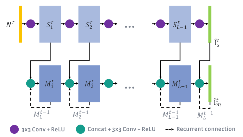
A natural approach, which is already popular in the natural language and audio processing literature [47], is to process temporal data with recurrent neural networks (RNN) modules [22]. RNNs operate on sequences and maintain an internal state which is combined with the input at each time step. In our model, we make use of recurrent connections to aggregate activations produced by our SFD network for each frame, as we show in Figure 1. This allows for an arbitrary input sequence length, our first goal. Unlike [5] and [42] which utilize a single-track network design, we use a two track network architecture with the top track dedicated to SFD and the bottom track dedicated to fusing those results into a final prediction for MFD.
By decoupling per-frame feature extraction from multi-frame aggregation, we enable the possibility for pre-training a network rapidly using only single-frame data. In practice, we found that this pre-training not only accelerates the learning process, but also produces significantly better results in terms of PSNR than when we train the entire MFD from scratch. The core intuition is that by first learning good features for SFD, we put the network in a good state for learning how to aggregate those features across observations, but still grant it the freedom to update those features by not freezing the SFD weights during training.
It is also important to note that the RNNs are connected in such a way as to permit the aggregation of observation features in several different ways. Temporal connections within the RNNs help aggregate information “across” frames, but lateral connections “within” the MFD track permit the aggregation of information at different physical scales and at different levels of abstraction.
4 Implementation and Results
To show that our method fulfills the goals set in Section 3, we evaluate it in multiple scenarios: single-image denoising, multi-frame denoising, and single-image super-resolution
4.1 Data
We trained all the networks in our evaluation using a dataset consisting of Apple Live Photos. Live Photos are burst sequences captured by Apple iPhone 6S and above111https://support.apple.com/en-us/HT207310. This dataset is very representative as it captures what mobile phone users like the photograph, and exhibits a wide range of scenes and motions. Approximately 73k public sequences were scraped from a social media website with a resolution of . We apply a burst stabilizer to each sequence, resulting in approximately 54.5k sequences successfully stabilized. In Section 4.2 we describe our stabilization procedure in more detail. 50k sequences were used for training with an additional 3.5k reserved for validation and 1k reserved for testing.
4.2 Stabilization
We implemented burst sequence stabilization using OpenCV222https://opencv.org/. In particular, we use a Lucas-Kanade tracker [29] to find correspondences between successive frames and then a rotation-only motion model and a static focal length guess to arrive at a homography for each frame. We warp all frames of a sequence back into a reference frame’s pose and crop and scale the sequence to maintain the original size and aspect ratio, but with the region of interest contained entirely within the valid regions of the warp. The stabilized sequences still exhibit some residual motion, either through moving objects or people, or through camera and scene motion which cannot be represented by a homography. This residual motion forces the network to adapt to non static scenes and be robust to motion, which is our 3rd goal.
4.3 Training details
We implemented the neural network from Section 3 using the Caffe2 framework333https://caffe2.ai/. Each model was trained using 4 Tesla M40 GPUs. As described in Section 3, training took place in two stages. First a single-frame model was trained. This model used a batch size of 128 and was trained for 500 epochs in approximately 5 hours. Using this single-frame model as initialization for the multi-frame (8-frame) model, we continue training with a batch size of 32 to accommodate the increased size of the multi-frame model over the single-frame model. This second stage was trained for 125 epochs in approximately 20 hours.
4.4 Noise modelling
We first evaluate our architecture using additive white Gaussian noise with and , in order to make comparison possible with previous methods, such as VBM4D. To be able to denoise real burst sequences, we modeled sensor noise following [13] and trained separate models by adding Poisson noise, labelled a in [13], with intensity ranging from 0.001 to 0.01 in linear space before converting back to sRGB and clipping. We also simulate Bayer filtering and reconstruct an RGB image using bilinear interpolation. Unless otherwise mentioned, we add synthetic noise before stabilization.
4.5 Single frame denoising
Here we compare our single frame denoiser with current state of the art methods on additive white Gaussian noise. We compare our own SFD, which is composed of 8 layers, with the two 20 layer networks of DenoiseNet (2017) [35] and DnCNN (2017) [48]. For the sake of comparison, we also include a 20 layer version of our SFD as well as reimplementations of both DnCNN and DenoiseNet. All models were trained for 2000 epochs on 8000 images from the PASCAL VOC2010 [11] using the training split from [35]. We also include in the comparison BM3D (2009) [8] and TNRD (2015) [6].
All models were tested on BSD68 [38], a set of 68 natural images from the Berkeley Segmentation Dataset [33]. In Figure 1, we can see diminishing returns in single frame denoising PSNR over the years, which confirms what Levin, et al. describe in [27], despite the use of deep neural networks. We can see that our simpler SFD 20 layers model only slightly underperforms both DenoiseNet and DnCNN by . However, as we show in the following section, the PSNR gains brought by multi-frame processing vastly outshine fractional single frame PSNR improvements.
| BM3D | 31.10 | 28.57 | 25.62 | 24.20 |
|---|---|---|---|---|
| TNRD | 31.41 | 28.91 | 25.95 | - |
| DenoiseNet [35] | 31.44 | 29.04 | 26.06 | 24.61 |
| DenoiseNet (reimpl) | 31.43 | 28.91 | 25.95 | 24.59 |
| DnCNN [48] | 31.73 | 29.23 | 26.23 | - |
| DnCNN (reimpl w/o BN) | 31.42 | 28.86 | 25.99 | 24.30 |
| SFD 8L | 31.15 | 28.63 | 25.65 | 24.11 |
| SFD 20L | 31.29 | 28.82 | 26.02 | 24.43 |
4.6 Burst denoising
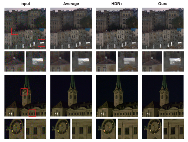
We evaluate our method on a held-out test set of Live Photos with synthetic additive white Gaussian noise added. In Table 3, we compare our architecture with single frame models as well as the multi-frame method VBM4D [32, 31]. We show qualitative results with in Figure 5. In Figures LABEL:fig:teaser and 8 we demonstrate that our method is capable of denoising real sequences. This evaluation was performed on real noisy bursts from HDR+ [18]. Please see our supplementary material for more results.
| C2F | C4F | C8F | Ours 4L | Ours 8L | Ours 12L | Ours 16L | Ours 20L | Ours nostab | |
| PSNR | 30.89 | 31.83 | 32.15 | 33.01 | 33.62 | 33.80 | 33.35 | 33.48 | 32.60 |
Ablation study
We now evaluate our architecture choices, where we compare our full model, with 8 layers and trained on sequences of 8 frames with other variants.
Concat We first compare our method with a naive multi-frame denoising approach, dubbed Concat, where the input consists of concatenated frames to a single pass denoiser. We evaluated this architecture with as well as and . As we can see in Table 2 this model performs significantly worse than our model.
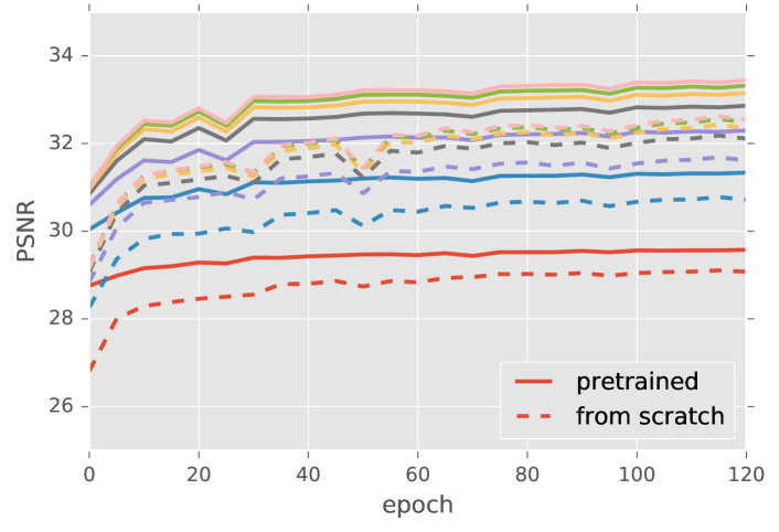
Number of layers We also evaluate the impact of the depth of the network by experimenting with and . As can be seen in Figure 2, the 16 and 20 layers network fail to surpass both the 8 and 12 layers after 125 epochs of training, likely due to the increased depth and parameter count. While the 12 layers network shows a marginal 0.18dB increase over the 8 layer model, we decided to go with the latter as we did not think that the modest increase in PSNR was worth the increase in both memory and computation time.
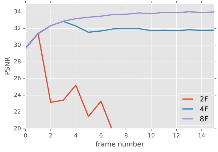
Length of training sequences Perhaps the most surprising result we encountered during training our recurrent model, was the importance of the number of frames in the training sequences. In Figure 3, we show that models trained on sequences of both 2 and 4 frames fail to generalize beyond their training length sequence. Only models trained with 8 frames were able to generalize to longer sequences at test time, and as we can see still denoise beyond 8 frames.
Pre-training One of the main advantages of using a two-track network is that we can train the SFD track independently first. As mentioned just before, a sequence length of 8 is required to ensure generalization to longer sequences, which makes the training of the full model much slower than training the single-frame pass. As we show in Figure 2, pre-training makes training the MFD significantly faster.
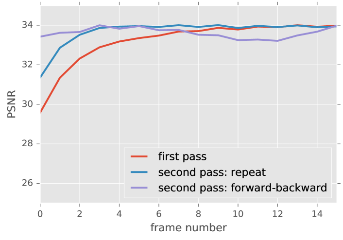
Frame ordering Due to its recurrent nature, our network exhibits a period of burn-in, where the first frames are being denoised to a lesser extent than the later ones. In order to denoise an entire sequence to a high quality level, we explored different options for frame ordering. As we show in Figure 4, by feeding the sequence twice to the network, we are able to obtain a higher average PSNR. We propose two variants, either repeat the sequence in the same order or reverse it the second time (named forward-backward). As we show in Figure 4, the forward-backward schedule does not suffer from burn-in nor flickering, thus meeting our 5th goal. We thus use forward-backward for all our experiments.
| Input | Average | VBM4D [32] | SFD (Ours) | MFD (Ours) | Ground truth |
|---|---|---|---|---|---|
 |
 |
 |
 |
 |
|
 |
 |
 |
 |
 |
| Bicubic | SFSR (Ours) | MFSR (Ours) | Ground truth |
|---|---|---|---|
 |
 |
 |
 |
 |
 |
 |
 |
| BM3D | 35.67 | 32.92 | 29.41 | 27.40 |
|---|---|---|---|---|
| VBM4D | 36.42 | 33.41 | 29.14 | 26.60 |
| DnCNN | 35.84 | 32.93 | 29.13 | 27.06 |
| DenoiseNet | 35.91 | 33.17 | 29.56 | 27.49 |
| Ours | 39.23 | 36.87 | 33.62 | 31.44 |
4.7 FlexISP
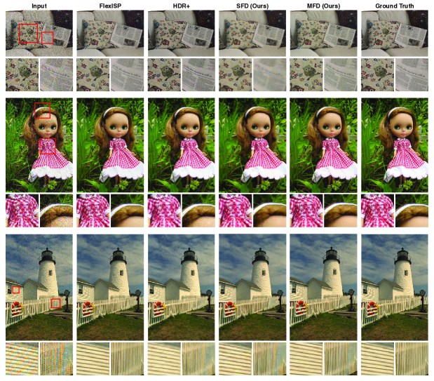
We now compare our method with other denoising approaches on the FlexISP dataset and show our results in Figure 7. Each sequence was denoised using the first 8 frames only. The synthetic sequences flickr doll and kodak fence were generated by randomly warping an input image and adding respectively additive and multiplicative white Gaussian noise of , and additive with Gaussian noise of as well as simulating a Bayer filter. We thus trained two models by replicating these conditions on our Live Photos dataset. On flickr doll our method achieves a PSNR of 29.39dB, matching FlexISP (dB) but falling short of ProxImaL (30.23dB), not shown here. On kodak fence our recurrent model achieves a 0.5dB advantage over FlexISP (34.44dB) with a PSNR of 34.976dB. Despite reaching a higher PSNR than FlexISP, our method does not mitigate the demosiacing artifacts on the fence, likely due to the absence of high frequency demosaicing artifacts in our training data.
4.8 Super resolution
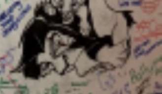
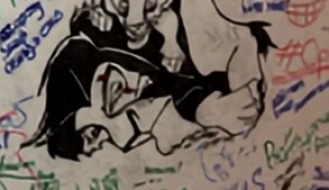
To illustrate that our approach generalizes to tasks beyond denoising, and our 6th goal, we trained our model to perform super-resolution, while keeping the rest of the training procedure identical to that of the denoising pipeline. Each input patch has been downsampled , using pixel area resampling and then resized to their original size using bilinear sampling. Figure 6 shows a couple of our results. Please refer to the supplemental material for more results.
5 Limitations
Our single-frame architecture, based on [35, 48, 26], makes use of stride-1 convolutions, enabling full-resolution processing across the entire network They are however both memory and computationally expensive, and have a small receptive field for a given network depth. Using multiscale architectures, such as a U-Nets [37], could help alleviate both issues, by reducing the computational and memory load, while increasing the receptive field. Finally while we trained our network on pre-stabilized sequences, we observed a significant drop in accuracy on unstabilized sequences, as can be seen in Table 2, as well as unstability on longer sequences. It would be interesting to train the network to stabilize the sequence by warping inside the network such as in [23, 16].
6 Conclusion
We have presented a novel deep neural architecture to process burst of images. We improve on a simple single frame architecture by making use of recurrent connections and show that while single-frame models are reaching performance limits for denoising, our recurrent architecture vastly outperform such models for multi-frame data. We carefully designed our method to align with the goals we stated in Section 3.1. As a result, our approach achieves state-of-the-art performance in our Live Photos dataset, and matches existing multi-frame denoisers on challenging existing datasets with real camera noise.
References
- [1] F. Agostinelli, M. R. Anderson, and H. Lee. Adaptive multi-column deep neural networks with application to robust image denoising. In C. J. C. Burges, L. Bottou, M. Welling, Z. Ghahramani, and K. Q. Weinberger, editors, Advances in Neural Information Processing Systems 26, pages 1493–1501. Curran Associates, Inc., 2013.
- [2] S. Borman and R. L. Stevenson. Super-resolution from image sequences-a review. In Circuits and Systems, 1998. Proceedings. 1998 Midwest Symposium on, pages 374–378. IEEE, 1998.
- [3] A. Buades, B. Coll, and J.-M. Morel. A non-local algorithm for image denoising. In Computer Vision and Pattern Recognition, 2005. CVPR 2005. IEEE Computer Society Conference on, volume 2, pages 60–65. IEEE, 2005.
- [4] H. C. Burger, C. J. Schuler, and S. Harmeling. Image denoising: Can plain neural networks compete with bm3d? In Computer Vision and Pattern Recognition (CVPR), 2012 IEEE Conference on, pages 2392–2399. IEEE, 2012.
- [5] C. R. A. Chaitanya, A. S. Kaplanyan, C. Schied, M. Salvi, A. Lefohn, D. Nowrouzezahrai, and T. Aila. Interactive reconstruction of monte carlo image sequences using a recurrent denoising autoencoder. ACM Transactions on Graphics (TOG), 36(4):98, 2017.
- [6] Y. Chen and T. Pock. Trainable nonlinear reaction diffusion: A flexible framework for fast and effective image restoration. IEEE transactions on pattern analysis and machine intelligence, 39(6):1256–1272, 2017.
- [7] K. Dabov, A. Foi, V. Katkovnik, and K. Egiazarian. Image denoising by sparse 3-d transform-domain collaborative filtering. IEEE Transactions on image processing, 16(8):2080–2095, 2007.
- [8] K. Dabov, A. Foi, V. Katkovnik, and K. Egiazarian. Bm3d image denoising with shape-adaptive principal component analysis. In SPARS’09-Signal Processing with Adaptive Sparse Structured Representations, 2009.
- [9] C. Dong, C. C. Loy, K. He, and X. Tang. Image super-resolution using deep convolutional networks. IEEE transactions on pattern analysis and machine intelligence, 38(2):295–307, 2016.
- [10] C. Dong, C. C. Loy, K. He, and X. Tang. Image super-resolution using deep convolutional networks. IEEE Transactions on Pattern Analysis and Machine Intelligence, 38(2):295–307, Feb 2016.
- [11] M. Everingham, L. Van Gool, C. K. I. Williams, J. Winn, and A. Zisserman. The pascal visual object classes (voc) challenge. International Journal of Computer Vision, 88(2):303–338, June 2010.
- [12] S. Farsiu, M. D. Robinson, M. Elad, and P. Milanfar. Fast and robust multiframe super resolution. IEEE transactions on image processing, 13(10):1327–1344, 2004.
- [13] A. Foi. Clipped noisy images: Heteroskedastic modeling and practical denoising. Signal Processing, 89(12):2609–2629, 2009.
- [14] M. Gharbi, G. Chaurasia, S. Paris, and F. Durand. Deep joint demosaicking and denoising. ACM Transactions on Graphics (TOG), 35(6):191, 2016.
- [15] D. Glasner, S. Bagon, and M. Irani. Super-resolution from a single image. In ICCV, 2009.
- [16] C. Godard, O. Mac Aodha, and G. J. Brostow. Unsupervised monocular depth estimation with left-right consistency. In The IEEE Conference on Computer Vision and Pattern Recognition (CVPR), July 2017.
- [17] S. W. Hasinoff, F. Durand, and W. T. Freeman. Noise-optimal capture for high dynamic range photography. In CVPR, pages 553–560. IEEE Computer Society, 2010.
- [18] S. W. Hasinoff, D. Sharlet, R. Geiss, A. Adams, J. T. Barron, F. Kainz, J. Chen, and M. Levoy. Burst photography for high dynamic range and low-light imaging on mobile cameras. ACM Transactions on Graphics (TOG), 35(6):192, 2016.
- [19] K. He, X. Zhang, S. Ren, and J. Sun. Deep residual learning for image recognition. In 2016 IEEE Conference on Computer Vision and Pattern Recognition (CVPR), pages 770–778, June 2016.
- [20] F. Heide, S. Diamond, M. Nießner, J. Ragan-Kelley, W. Heidrich, and G. Wetzstein. Proximal: Efficient image optimization using proximal algorithms. ACM Transactions on Graphics (TOG), 35(4):84, 2016.
- [21] F. Heide, M. Steinberger, Y.-T. Tsai, M. Rouf, D. Pajak, D. Reddy, O. Gallo, J. Liu, W. Heidrich, K. Egiazarian, et al. Flexisp: A flexible camera image processing framework. ACM Transactions on Graphics (TOG), 33(6):231, 2014.
- [22] J. J. Hopfield. Neural networks and physical systems with emergent collective computational abilities. Proceedings of the national academy of sciences, 79(8):2554–2558, 1982.
- [23] M. Jaderberg, K. Simonyan, A. Zisserman, et al. Spatial transformer networks. In Advances in Neural Information Processing Systems, pages 2017–2025, 2015.
- [24] V. Jain and S. Seung. Natural image denoising with convolutional networks. In D. Koller, D. Schuurmans, Y. Bengio, and L. Bottou, editors, Advances in Neural Information Processing Systems 21, pages 769–776. Curran Associates, Inc., 2009.
- [25] D. P. Kingma and J. Ba. Adam: A method for stochastic optimization. In Proceedings of the 3rd International Conference on Learning Representations (ICLR), 2014.
- [26] C. Ledig, L. Theis, F. Huszar, J. Caballero, A. Cunningham, A. Acosta, A. Aitken, A. Tejani, J. Totz, Z. Wang, and W. Shi. Photo-realistic single image super-resolution using a generative adversarial network. In The IEEE Conference on Computer Vision and Pattern Recognition (CVPR), July 2017.
- [27] A. Levin and B. Nadler. Natural image denoising: Optimality and inherent bounds. In Computer Vision and Pattern Recognition (CVPR), 2011 IEEE Conference on, pages 2833–2840. IEEE, 2011.
- [28] Z. Liu, L. Yuan, X. Tang, M. Uyttendaele, and J. Sun. Fast burst images denoising. ACM Transactions on Graphics (TOG), 33(6):232, 2014.
- [29] B. D. Lucas and T. Kanade. An iterative image registration technique with an application to stereo vision. In Proceedings of the 7th International Joint Conference on Artificial Intelligence - Volume 2, IJCAI’81, pages 674–679, San Francisco, CA, USA, 1981. Morgan Kaufmann Publishers Inc.
- [30] A. L. Maas, A. Y. Hannun, and A. Y. Ng. Rectifier nonlinearities improve neural network acoustic models. In Proc. ICML, volume 30, 2013.
- [31] M. Maggioni, G. Boracchi, A. Foi, and K. Egiazarian. Video denoising, deblocking, and enhancement through separable 4-d nonlocal spatiotemporal transforms. IEEE Transactions on image processing, 21(9):3952–3966, 2012.
- [32] M. Maggioni, G. Boracchi, A. Foi, and K. O. Egiazarian. Video denoising using separable 4d nonlocal spatiotemporal transforms. In Image Processing: Algorithms and Systems, page 787003, 2011.
- [33] D. Martin, C. Fowlkes, D. Tal, and J. Malik. A database of human segmented natural images and its application to evaluating segmentation algorithms and measuring ecological statistics. In Computer Vision, 2001. ICCV 2001. Proceedings. Eighth IEEE International Conference on, volume 2, pages 416–423. IEEE, 2001.
- [34] K. Nasrollahi and T. B. Moeslund. Super-resolution: a comprehensive survey. Machine vision and applications, 25(6):1423–1468, 2014.
- [35] T. Remez, O. Litany, R. Giryes, and A. M. Bronstein. Deep class aware denoising. arXiv preprint arXiv:1701.01698, 2017.
- [36] O. Ronneberger, P. Fischer, and T. Brox. U-Net: Convolutional Networks for Biomedical Image Segmentation, pages 234–241. Springer International Publishing, Cham, 2015.
- [37] O. Ronneberger, P. Fischer, and T. Brox. U-net: Convolutional networks for biomedical image segmentation. In International Conference on Medical Image Computing and Computer-Assisted Intervention, pages 234–241. Springer, 2015.
- [38] S. Roth and M. J. Black. Fields of experts: A framework for learning image priors. In Computer Vision and Pattern Recognition, 2005. CVPR 2005. IEEE Computer Society Conference on, volume 2, pages 860–867. IEEE, 2005.
- [39] E. Shelhamer, J. Long, and T. Darrell. Fully convolutional networks for semantic segmentation. IEEE Transactions on Pattern Analysis and Machine Intelligence, 39(4):640–651, April 2017.
- [40] M. Tico. Multi-frame image denoising and stabilization. In Signal Processing Conference, 2008 16th European, pages 1–4. IEEE, 2008.
- [41] P. J. Werbos. Generalization of backpropagation with application to a recurrent gas market model. Neural networks, 1(4):339–356, 1988.
- [42] P. Wieschollek, M. Hirsch, B. Scholkopf, and H. P. A. Lensch. Learning blind motion deblurring. In The IEEE International Conference on Computer Vision (ICCV), Oct 2017.
- [43] J. Xie, L. Xu, and E. Chen. Image denoising and inpainting with deep neural networks. In F. Pereira, C. J. C. Burges, L. Bottou, and K. Q. Weinberger, editors, Advances in Neural Information Processing Systems 25, pages 341–349. Curran Associates, Inc., 2012.
- [44] X. Y. Xinyuan Chen, Li Song. Deep rnns for video denoising. In Proc.SPIE, volume 9971, pages 9971 – 9971 – 10, 2016.
- [45] C.-Y. Yang, C. Ma, and M.-H. Yang. Single-image super-resolution: A benchmark. In European Conference on Computer Vision, pages 372–386. Springer, 2014.
- [46] J. Yang, J. Wright, T. S. Huang, and Y. Ma. Image super-resolution via sparse representation. IEEE transactions on image processing, 19(11):2861–2873, 2010.
- [47] W. Yin, K. Kann, M. Yu, and H. Schütze. Comparative study of cnn and rnn for natural language processing. arXiv preprint arXiv:1702.01923, 2017.
- [48] K. Zhang, W. Zuo, Y. Chen, D. Meng, and L. Zhang. Beyond a gaussian denoiser: Residual learning of deep cnn for image denoising. IEEE Transactions on Image Processing, 26:3142–3155, 2017.
- [49] K. Zhang, W. Zuo, S. Gu, and L. Zhang. Learning deep cnn denoiser prior for image restoration. In The IEEE Conference on Computer Vision and Pattern Recognition (CVPR), July 2017.
- [50] H. Zhao, O. Gallo, I. Frosio, and J. Kautz. Loss functions for image restoration with neural networks. IEEE Transactions on Computational Imaging, 3(1):47–57, 2017.