On the Prediction of 100 MeV Solar Energetic Particle Events Using GOES Satellite Data
Abstract
Solar energetic particles are a result of intense solar events such as solar flares and Coronal Mass Ejections (CMEs). These latter events all together can cause major disruptions to spacecraft that are in Earth’s orbit and outside of the magnetosphere. In this work we are interested in establishing the necessary conditions for a major geo-effective solar particle storm immediately after a major flare, namely the existence of a direct magnetic connection. To our knowledge, this is the first work that explores not only the correlations of GOES X-ray and proton channels, but also the correlations that happen across all the proton channels. We found that proton channels auto-correlations and cross-correlations may also be precursors to the occurrence of an SEP event. In this paper, we tackle the problem of predicting 100 MeV SEP events from a multivariate time series perspective using easily interpretable decision tree models.
Index Terms:
SEP Events Prediction; CART decision tree, 100 MeV SEP; GOES X-ray and Proton correlation; Vector autoregressionI Introduction
The occurence of important Solar Energetic Particle (SEP) events is one of the prominent planning considerations for manned and unmanned lunar and planetary missions [1]. A high exposure to large solar particles events can deliver critical doses to human organs and may damage the instruments on board of satellites and the global positioning system (GPS) due to the risk of saturation. SEP events usually happen 30 minutes after the occurrence of the X-ray flare, which leaves very little time for astronauts performing extra-vehicular activity on the International Space Station or planetary surfaces to take evasive actions [2]. Earlier warning of the SEP events will be a valuable tool for mission controllers that need to take a prompt decision concerning the atrounauts’ safety and the mission completion. When a solar flare or a CME happens, the magnetic force that is exercised is manifested through different effects. Some of the effects are listed in their order of occurrence: light, thermal, particle acceleration, and matter ejection in case of CMEs. The first effect of a solar flare is a flash of increased brightness that is observed near the Sun’s surface which is due to the X-rays and UV radiation. Then, part of the magnetic energy is converted into thermal energy in the area where the eruption happened. Solar particles in the atmosphere are then accelerated with different speed spectra, that can reach up to 80% of the speed of light, depending on the intensity of the parent eruptive event.
Finally, in the case of a CME, plasma and magnetic field from the solar corona is released into the solar wind. Though most of the solar particles have the same composition, they are labeled differently depending on their energies starting from 1 keV, in the solar wind, to more than 500 MeV. SEP events are composed of particles, predominantly protons and electrons, with at least 1 MeV energy that last between 2-20 days and have a range of fluxes of 5-6 orders of magnitude [4]. Only 100 MeV particles are discussed herein. It is generally accepted that there are two types of SEP events, one is associated with CMEs and the other is associated with flares that are called respectively gradual and impulsive [5].
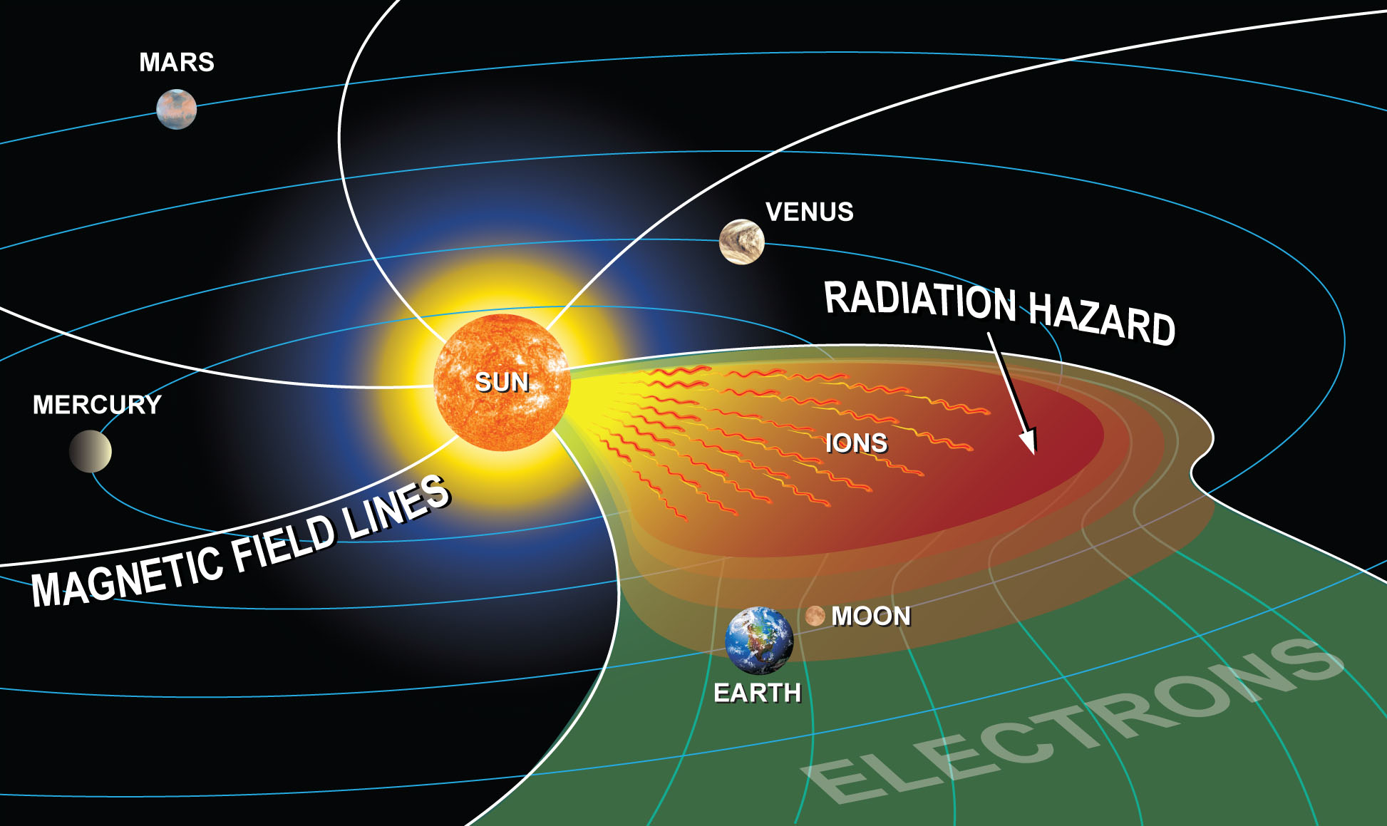
In this paper, we propose a novel method for predicting SEP events 100 MeV based on the proton and X-ray correlations time series using interpretable decision tree models. Predicting impulsive events is considered to be a more challenging problem than predicting the gradual events that happen progressively and leave a large window for issuing SEP warnings. While we are mainly concerned with impulsive events, we used the gradual events as well to test our model with. The accelerated impulsive events may or may not reach Earth depending on the location of their parent event because their motion is confined by the magnetic field. More specifically, in order for the accelerated particles to reach Earth, a Sun-Earth magnetic connection needs to exist that allows the particles to flow to Earth via the Parker spiral. Fig .1 shows a cartoon of a solar eruption that happened in the Western limb of the Sun that happens to be magnetically connected to Earth.
Since SEP events are also part of solar activity, it may seem that their occurrence is dependent on the solar cycle and therefore the number of Sunspots on the Sun’s surface, which is the case for other solar eruptions. However, according to [4], there is no correlation between the solar cycle and SEP event occurrence and fluences. In addition, there is no evidence the dependence of SEP events on the number of Sunspots that are present during that snapshot in time [4].
The rest of the paper is presented as follows. In Section 2 we provide background material on the SEP predictive models and related works. Section 3 defines our dataset used in this study, and then in Section 4 we lay out our methodology. Finally, Section 5 contains our experimental results, and we finish with conclusions and future work in Section 6.
II Related Works
There are a number of predictive models of SEP events that can be categorized into two classes: physics-based models [6, 7] and the precursor-based models [8, 9]. The first category of models includes the SOLar Particle Engineering Code (SOLPENCO) that can predict the flux and fluence of the gradual SEP events originating from CMEs [10]. However, such efforts mainly focus on gradual events. On the other hand, there are models that rely on historical observations to find SEP events associated precursors. One example of such systems is the proton prediction system (PPS), which is a program developed at the Air Force Research Laboratory (AFRL), that predicts low energy SEP events E{5, 10, 50} MeV, composition, and intensities. PPS assumes that there is a relationship between the proton flux and the parent flare event. PPS takes advantage of the correlation between large SEP events observed by the Interplanetary Monitoring Platform (IMP) satellites as well as their correlated flare signatures captured by GOES proton, X-ray flux and H flare location [11]. Also, the Relativistic Electron Alert System for Exploration (RELEASE), predicts the intensity of SEP events using relativistic near light speed electrons [1]. RELEASE uses electron flux data from the SOHO/COSTEP sensor of the range of 0.3-1.2 MeV to forecast the proton intensity of the energy range 30-50 MeV. Another example of precursor-based models appear in [12], that base their study on the ”big flare syndrome”. This latter theory states that SEP events occurrence at 1 AU is highly probable when the intensity of the parent flare is high. Following this assumption, the authors in [12] issue SEP forecasts for important flares greater than M2. To this end, it uses type III radio burst data, H data, and GOES soft X-ray data. Finally, , is an operational system that uses a ground-based neutron monitor (MNDB, www.nmdb.com) to issue alerts of SEP events of energies E433 MeV. Finally, the University of Malaga Solar Energetic Particles Prediction (UMASEP) is another system that first predicts whether a 10 MeV and 100 MeV SEP will happen or not. To do so, it computes the correlation between the soft X-ray and proton channels to assess if there is a magnetic connection between the Sun and Earth at the time of the X-ray event. Then, in case of existence of magnetic connection, UMASEP gives an estimation on the time when the proton flux is expected to surpass the SWPC threshold of J(E 10MeV)= 10 and J(E 100MeV)= 1 (1 = ) and for the case of UMASEP-100, the intensity of the first three hours after the event onset time.
While most of the SEP predictive systems either focus on the CME associated events or low energy SEP events, with the exception of and UMASEP, in this present work, we focus on higher energy SEP events that can be more disruptive than lower energy events. In this work, we study the GOES cross-channel correlations that can give an early insight on whether there exist a magnetic connection or not.
We aim to provide an interpretable decision tree models using a balanced dataset of SEP and non-SEP events. The highest SEP energy band of 500 MeV or higher that are measurable from the ground is out of the scope of this study. Similarly, the lower SEP energy band of 100 MeV is not considered in this study.
III Data
Our dataset is composed of multivariate time series of X-ray, integral proton flux and fluences spectra that were measured on board of Space Environment Monitor (SEM) instruments package of the Geostationary Operational Earth Satellites (GOES). In particular, we consider both the short and long X-ray channel data recorded by the X-ray Sensor (XRS). For the proton channels, we consider channels P6 and P7 recorded by the Energetic Particle Sensor (EPS) and proton channels P8, P9, P10, and P11 recorded by the High Energy Proton and Alpha Detector (HEPAD). Table I summarizes the instruments onboard the GOES satellites and their corresponding data channels that we used.
| Fast-Rising | Slow-Rising | Lack of SEP |
|---|---|---|
 |
 |
 |
 |
 |
 |
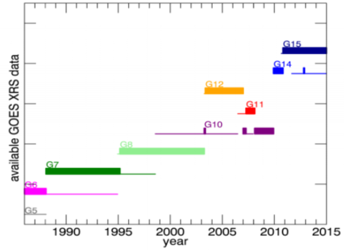
The data we collected is made publically available by NOAA in the following link: (https://satdat.ngdc.noaa.gov/sem/goes/data/new_avg/).The data is available in three different cadences. The full resolution data is captured every three seconds from the GOES satellites, which is aggregated and made available with one and five minute cadences. In this paper we use the aggregated five minute data which is the one usually cited in the literature [13] [14] [15]. In most cases, there are a couple a co-existing GOES satellites whose data is captured by more than one GOES satellite at a time. In this study, we always consider the data reported by the primary GOES satellite that is designated by the NOAA, as illustrated in Fig .2. The latter figure shows the primary GOES satellite with a bold line and the other co-existing GOES for every year. GOES-13 measurements were unstable for many years, but have been stable since 2014.
| Instrument | Channels | Description |
|---|---|---|
| XRS | xs | Short wavelength channel irradiance (0.5 - 0.3 nm) |
| xl | Long wavelength channel irradiance (0.1-0.8 nm) | |
| HEPAD | p8_flux | Proton Channel 350.0 - 420.0 MeV |
| p9_flux | Proton Channel 420.0 - 510.0 MeV | |
| p10_flux | Proton Channel 510.0 - 700.0 MeV | |
| p11_flux | Proton Channel 700.0 MeV | |
| EPS | p6_flux | Proton Channel 80.0 - 165.0 MeV |
| p7_flux | Proton Channel 165.0 - 500.0 MeV |
| SEP Event ID | Onset Time of SEP Event | Parent X-ray Event |
|---|---|---|
| 1 | 1997-11-04 05:52:00 | 1997-11-04 05:52:00 |
| 2 | 1997-11-06 11:49:00 | 1997-11-06 11:49:00 |
| 3* | 1998-04-20 09:38:00 | 1998-04-20 09:38:00 |
| 4 | 1998-05-02 13:31:00 | 1998-05-02 13:31:00 |
| 5 | 1998-05-06 07:58:00 | 1998-05-06 07:58:00 |
| 6 | 1998-08-24 21:50:00 | 1998-08-24 21:50:00 |
| 7 | 1998-09-30 13:50:00 | 1998-09-30 13:50:00 |
| 8 | 1998-11-14 05:15:00 | 1998-11-14 06:05:00 |
| 9 | 2000-06-10 16:40:00 | 2000-06-10 16:40:00 |
| 10 | 2000-07-14 10:03:00 | 2000-07-14 10:03:00 |
| 11 | 2000-11-08 22:42:00 | 2000-11-08 22:42:00 |
| 12 | 2000-11-24 14:51:00 | 2000-11-24 14:51:00 |
| 13* | 2000-11-26 16:34:00 | 2000-11-26 16:34:00 |
| 14* | 2001-04-02 21:32:00 | 2001-04-02 21:32:00 |
| 15 | 2001-04-12 09:39:00 | 2001-04-12 09:39:00 |
| 16 | 2001-04-15 13:19:00 | 2001-04-15 13:19:00 |
| 17 | 2001-04-17 21:18:00 | 2001-04-18 02:05:00 |
| 18 | 2001-08-15 12:38:00 | 2001-08-16 23:30:00 |
| 19* | 2001-09-24 09:32:00 | 2001-09-24 09:32:00 |
| 20 | 2001-11-04 16:03:00 | 2001-11-04 16:03:00 |
| 21 | 2001-11-22 22:32:00 | 2001-11-22 19:45:00 |
| 22 | 2001-12-26 04:32:00 | 2001-12-26 04:32:00 |
| 23 | 2002-04-21 00:43:00 | 2002-04-21 00:43:00 |
| 24 | 2002-08-22 01:47:00 | 2002-08-22 01:47:00 |
| 25 | 2002-08-24 00:49:00 | 2002-08-24 00:49:00 |
| 26 | 2003-10-28 09:51:00 | 2003-10-28 09:51:00 |
| 27 | 2003-11-02 17:03:00 | 2003-11-02 17:03:00 |
| 28* | 2003-11-05 02:37:00 | 2003-11-05 02:37:00 |
| 29+ | 2004-11-01 03:04:00 | 2004-11-01 03:04:00 |
| 30+ | 2004-11-10 01:59:00 | 2004-11-10 01:59:00 |
| 31+ | 2005-01-16 21:55:00 | 2005-01-17 08:00:00 |
| 32+ | 2005-01-20 06:36:00 | 2005-01-20 06:36:00 |
| 33+ | 2005-06-16 20:01:00 | 2005-06-16 20:01:00 |
| 34+ * | 2005-09-07 17:17:00 | 2005-09-07 17:17:00 |
| 35+ * | 2006-12-06 18:29:00 | 2006-12-06 18:29:00 |
| 36+ | 2006-12-13 02:14:00 | 2006-12-13 02:14:00 |
| 37+ | 2006-12-14 21:07:00 | 2006-12-14 21:07:00 |
| 38 | 2011-06-07 06:16:00 | 2011-06-07 06:16:00 |
| 39 | 2011-08-04 03:41:00 | 2011-08-04 03:41:00 |
| 40 | 2011-08-09 07:48:00 | 2011-08-09 07:48:00 |
| 41 | 2012-01-23 03:38:00 | 2012-01-23 03:38:00 |
| 42* | 2012-01-27 17:37:00 | 2012-01-27 17:37:00 |
| 43 | 2012-03-07 01:05:00 | 2012-03-07 01:05:00 |
| 44 | 2012-03-13 17:12:00 | 2012-03-13 17:12:00 |
| 45 | 2012-05-17 01:25:00 | 2012-05-17 01:25:00 |
| 46* | 2013-04-11 06:55:00 | 2013-04-11 06:55:00 |
| 47 | 2013-05-22 13:08:00 | 2013-05-22 13:08:00 |
-
*
Gradual Events.
-
+
Missing Data in P6 and P7.
| Non SEP Event ID | X-ray Event | Class |
|---|---|---|
| 1 | 1997-09-24 02:43:00 | M59 |
| 2 | 1997-11-27 12:59:00 | X26 |
| 3 | 1997-11-28 04:53:00 | M68 |
| 4 | 1997-11-29 22:28:00 | M64 |
| 5 | 1998-07-14 12:51:00 | M46 |
| 6 | 1998-08-18 08:14:00 | X28 |
| 7 | 1998-08-18 22:10:00 | X49 |
| 8 | 1998-08-19 21:35:00 | X39 |
| 9 | 1998-11-28 04:54:00 | X33 |
| 10 | 1999-01-16 12:02:00 | M36 |
| 11 | 1999-04-03 22:56:00 | M43 |
| 12 | 1999-04-04 05:15:00 | M54 |
| 13 | 1999-05-03 05:36:00 | M44 |
| 14 | 1999-07-19 08:16:00 | M58 |
| 15 | 1999-07-29 19:31:00 | M51 |
| 16 | 1999-08-20 23:03:00 | M98 |
| 17 | 1999-08-21 16:30:00 | M37 |
| 18 | 1999-08-21 22:10:00 | M59 |
| 19 | 1999-08-25 01:32:00 | M36 |
| 20 | 1999-10-14 08:54:00 | X18 |
| 21 | 1999-11-14 07:54:00 | M80 |
| 22 | 1999-11-16 02:36:00 | M38 |
| 23 | 1999-11-17 09:47:00 | M74 |
| 24 | 1999-12-22 18:52:00 | M53 |
| 25 | 2000-01-18 17:07:00 | M39 |
| 26 | 2000-02-05 19:17:00 | X12 |
| 27 | 2000-03-12 23:30:00 | M36 |
| 28 | 2000-03-31 10:13:00 | M41 |
| 29 | 2000-04-15 10:09:00 | M43 |
| 30 | 2000-06-02 06:52:00 | M41 |
| 31 | 2000-06-02 18:48:00 | M76 |
| 32 | 2000-10-29 01:28:00 | M44 |
| 33 | 2000-12-27 15:30:00 | M43 |
| 34 | 2001-01-20 21:06:00 | M77 |
| 35 | 2001-03-28 11:21:00 | M43 |
| 36 | 2001-06-13 11:22:00 | M78 |
| 37 | 2001-06-23 00:10:00 | M56 |
| 38 | 2001-06-23 04:02:00 | X12 |
| 39+ | 2004-12-30 22:02:00 | M42 |
| 40+ | 2004-01-07 03:43:00 | M45 |
| 41+ | 2004-09-12 00:04:00 | M48 |
| 42+ | 2004-01-17 17:35:00 | M50 |
| 43+ | 2005-07-27 04:33:00 | M37 |
| 44+ | 2005-11-14 14:16:00 | M39 |
| 45+ | 2005-08-02 18:22:00 | M42 |
| 46+ | 2005-07-28 21:39:00 | M48 |
| 47+ | 2006-04-27 15:22:00 | M79 |
-
+
Missing Data in P6 and P7.
Only a portion of the collected data is used to train and test our classifier. The positive class in this study is composed of X-Ray and proton channels time series that led to 100 MeV SEP impulsive or gradual events. On the other hand, the negative class is composed of X-Ray and proton channels time series that did not lead to any 100 MeV SEP events. In order to select such events we used a number of catalogs. For the positive class events we used the same catalog of SEP events 100 MeV in [15] that covers the events that happened between 1997 and 2013.
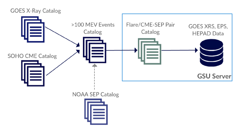
Our positive class is composed of the 47 X-Ray parent events of their corresponding 100 MeV SEP events that appear in [15] and shown in Table II. We use the X-Ray catalog (https://www.ngdc.noaa.gov/stp/space-weather/solar-data/solar-features/solar-flares/x-rays/goes/xrs/) as well as the CME catalog (https://cdaw.gsfc.nasa.gov/CME_list/) from the SOlar Heliospheric Observatory (SOHO) to derive the parent events of the 100 MeV SEP events. There was an exception of two SEP events that happened in August and September 1998 that we believe are gradual events but could not map to any CME report due to the missing data during the SOHO mission interruption. This latter happened because of the major loss of altitude experienced by the spacecraft due to the failure to adequately monitor the spacecraft status, and an erroneous decision which disabled part of the on-board autonomous failure detection [15]. It is worth to note that we consulted the NOAA-prepared SEP events catalog along with their parent flare/CME events (ftp://ftp.swpc.noaa.gov/pub/indices/SPE.txt). For the case of events that are missing the NOAA catalog, we made our own flare/CME-SEP events mapping. Fig. 3 shows the three external catalogs that we used to produce our own catalog from which we generate our SEP dataset. To obtain a balanced dataset, we selected another 47 X-ray events that did not produce any SEP events that is, shown in Table III. We noticed that there are nine SEP events (refer Table II ID:29-37) that happened during the period when only GOES-12 was operational as can be seen in Fig. 2. At that period, channels P6 and P7 failed and there was no secondary GOES. To make sure not to create any biased classifier that relies on the missing data to make the prediction, we made sure to choose nine events from the negative class as well that did not produce any SEP event (see Table III ID:39-47).
In this paper we make a clear distinction between the two different classes of SEP events: gradual and impulsive. We assume that an SEP event is flare accelerated, and therefore impulsive, if the lag between the flare occurrence and the SEP onset time is very small and the peak flux intensity has reached a global peak few minutes to an hour after the onset time. On the other hand, a gradual event shows a progressive increase in the proton flux trend that does not reach a global peak; instead, the peak is maintained steadily before dropping again progressively. Finally, a non-SEP event happens when there is an X-ray event of minimum intensity that is not followed by any significant proton flux increase in one of the P6-P11 channels.
IV Methodology
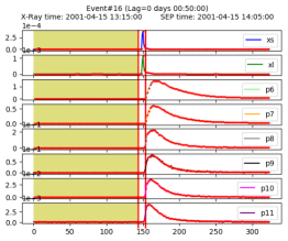
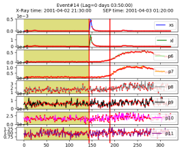
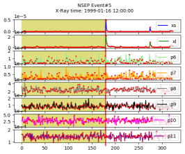
This section introduces a novel approach in predicting the occurrence of 100 MeV SEP events based on interpretable decision tree models. We considered the X-ray and proton channels as multivariate time series that entail some correlations which may be precursors to the occurrence of an event. While [15] considers the correlation between the X-ray and proton channels only, we extended the correlation study into all the channels, including correlations that happen across different proton channels. We approached the problem from a multivariate time series classification perspective. The classification task being whether the observed time series windows will lead to an SEP event or not. There are two ways of performing a time series classification. The first approach, which first appeared in [16], is to use the raw time series data and find the K-nearest-neighbor with a similarity measures such as Euclidean distance, and dynamic time warping. This approach is effective when the time series of the same label shows a distinguishable similar shape pattern. In this problem, the time series that we are working with are direct instruments readings that show a jitter effect, which is common in electromechanical device readings [17]. An example of the jitter effect is shown in P10, and P11 in Figure. 4-b and Figure. 4-c. Time series jitter makes it hard for distance measures, including elastic measures, to capture similar shape patterns. Therefore, we explored the second time series classification approach that relies on extracting features from the raw time series before feeding it to a model. In the next subsections, we will talk about the time series data extraction, the feature generation and data pre-processing.
IV-A Data Extraction
Our approach starts from the assumption that a 100 MeV impulsive event may occur if the parent X-ray event peak is at least as was suggested in [15]. Therefore we carefully picked the negative class an X-ray event whose peak intensity is at least but did not lead to any SEP event (refer column 3 in Table III). We extracted different observation windows of data that we call a span. A span is defined as the number of hours that constitute the observation period prior to an X-ray event. A total of 94 (47*2) X-ray events (shown in column 3 and column 2 of Table .II and Table .III respectively) were extracted with different span windows. The span concept is illustrated in the yellow shaded area in Figure. 4. The span window, in this case is 10 hours and stops exactly at the start time of the X-ray event. As we considered the five minutes as the cadence between reports, a 10-hour span window represents a 120-length multivariate X-ray and proton time series.
IV-B Feature Generation
To express the X-ray and proton cross-channel correlations we used a Vector Autoregression Model (VAR) which is a stochastic process model used to capture the linear interdependencies among multiple time series. VAR is the extension of the univariate autoregressive model to multivariate time series. The VAR model is useful for describing the behavior of economic, financial time series and for forecasting [18]. The VAR model permits us to express each time series window as a linear function of past lags (values in the past) of itself and of past lags of the other time series. The lag signifies the factor by which we multiply a value of a time series to produce its previous value in time. Theoretically, if there exists a magnetic connection between the Sun and Earth through the Parker spiral, the X-ray fluctuation precedes its corresponding proton fluctuation. Therefore, we do not express the X-ray channels in terms of the other time series, but, we focus on expressing the proton channels with respect to the past lags of themselves and with past lags of the X-ray channels (xs and xl). The VAR model of order one, denoted as VAR(1) in our setting can be expressed by Equations.(1)-(6).
There is a total of eight time series that represent the proton channels. Every equation highlights the relationship between the dependent variable and the other protons and X-ray variables, which are independent variables. The higher the dependence of a proton channel on an independent variable, the higher is the magnitude of the coefficient . We used the coefficients of the proton equations as a feature vector representing a data sample. The feature vector representing a data point using the VAR(n) model is expressed in Equation.7.
Since the lag parameter determines the number of coefficients involved in the equation, the number of features in the feature vector varies. More specifically, the total number of features are 8 (independent variables) * 6 (dependent variables).
| (1) |
| (2) |
| (3) |
⋮
| (6) |
| (7) |
IV-C Data Preprocessing
Before feeding the data to a classifier we cleaned the data from empty values that appear in the generated features. To do so, we used the 3-nearest neighbors class-level imputation technique. The method finds the 3 nearest neighbors that have the same label of the sample with the missing feature. Nearest neighbors imputation weights the samples using the mean squared difference on features based on the other non-missing features. Then it imputes the missing value with the nearest neighbor sample. The reason why the imputation is done on a class level basis is that features may behave differently across the two classes (SEP and non-SEP), therefore; it is important to impute the missing data with the same class values.
V Experimental Evaluation
In this section we explain the decision tree model that we will be using as well as the sampling methodology. We will also provide a rationale for the choice of parameters ( and ). Finally we will zoom in the best model with the most promising performance levels.
V-A Decision Tree Model
A decision tree is a hierarchical tree structure used to determine classes based on a series of rules/questions about the attribute values of the data points [19]. Every non-leaf node represents an attribute split (question) and all the leaf nodes represent the classification result. In short, given a set of features with their corresponding classes a decision tree produces a sequence of questions that can be used to recognize the class of a data sample. In this paper, the data attributes are the VAR() coefficients and the classes are binary: SEP and non-SEP.
The decision tree classification model first starts by finding the variable that maximizes the separation between classes. Different algorithms use different metrics, also called purity measures, for measuring the feature that maximizes the split. Some splitting criteria include Gini impurity, information gain, and variance reduction. The commonality between these metrics is that they all measure the homogeneity of a given feature with respect to the classes. The metric is applied to each candidate feature to measure the quality of the split, and the best feature is used. In this paper we used the CART decision tree algorithm, as appeared in [20] and [21], with Gini and information gain as the splitting criteria.
V-B Parameter Choice
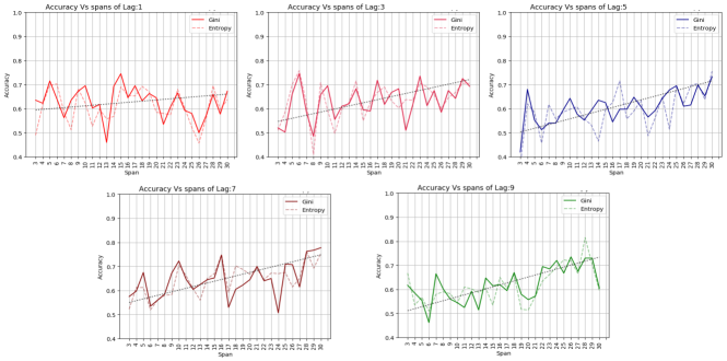
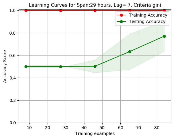
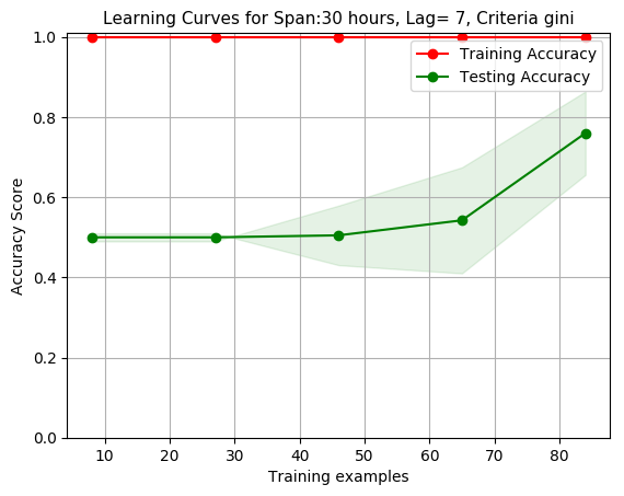
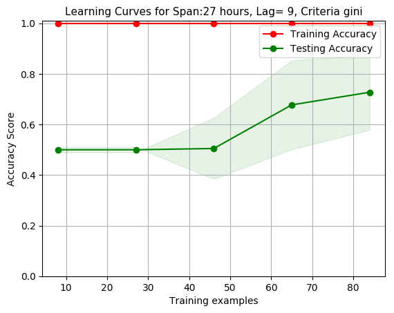
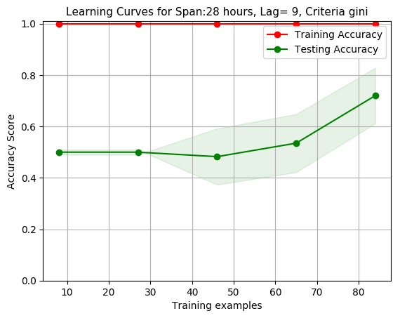
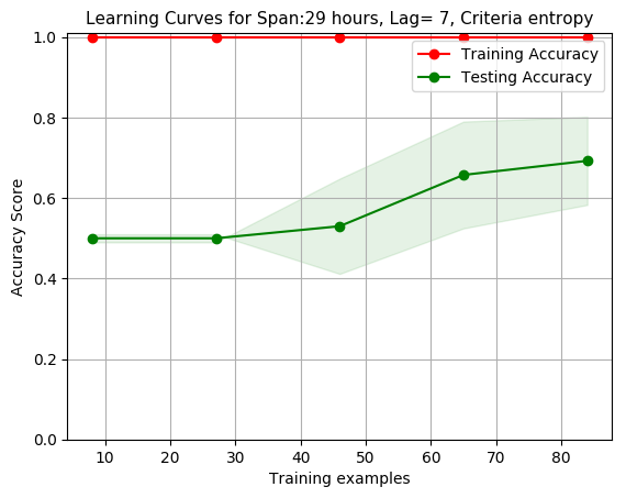
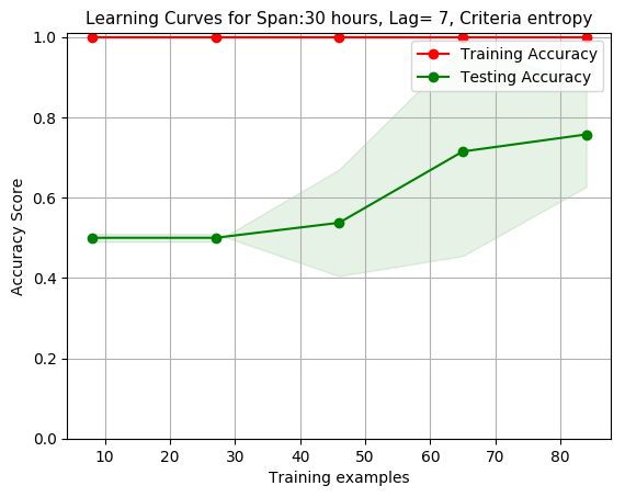
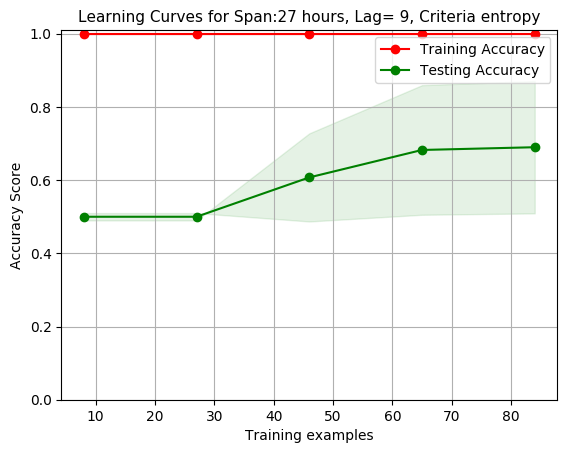
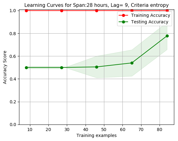
Our approach relies heavily on the choice of parameters, namely, the span window and the VAR model lag parameter. The span is the number of observation hours that precede the occurrence of an X-ray event. The latter determines the length of the multivariate time series to be extracted. On the other hand, the lag () determines the size of the feature space that will be used as well as the length of the dependence of the time series with each other in the past. As mentioned previously, with a one-step increment of the lag parameter the size of the feature space almost doubles = 8*(independent variables)*6 (equations)*+6*(equations). In order to determine the optimal parameters to be used, we run a decision tree model on a set of values for both the span and lag parameters. More specifically, we used the range [3-30] for the span window and the set {1,3,5,7,9} for . Since we have a balanced dataset we used a stratified Ten-fold cross validation as the sampling methodology. A stratified sampling always ensures a balance in the number of positive and negative samples for both the training and testing data samples. Ten-fold cross-validation randomly splits the data into 10 subsets, models are trained with nine of the folds (90% of the dataset), and test it with one fold (10% of the dataset). Every fold is used once for testing and nine times for training. In our experiments, we report the average accuracy on the 10 folds. Fig. 5 illustrates the accuracy curves with respect to the span windows for the five lags that we considered. We reported the accuracies of the decision tree model using both gini and information gain splitting criteria. In order to better capture the model behavior with the increasing span we plotted a linear fit to the accuracy curves of each lag. The first observation that can be made is that the slopes of the linear fit for =1 and =3 are relatively small in comparison to the other lags (3). This signifies that the model does not show any increasing or decreasing accuracy trend with the increase of the span window. Therefore we conclude that =1 and =3 are too small to discover any relationship between the proton and X-ray channels. Having the lag parameter set to =1 and =3 corresponds to expressing the time series (independent variable) going back in time up to five minute and 15 minutes respectively. These latter times are small, especially for =1 (5 minutes), which theoretically is not possible since the protons can at most reach the speed of light that corresponds to a lag of at least 8.5 minutes. For the other lags () there is noticeable increase in steepness in the accuracy linear fit which suggests that the accuracy increases with the increasing span window. The second observation is that for all the datasets the best accuracy was achieved in the last four span window (i.e span {27,28,29,30}). Therefore, we filtered the initial range of parameter values to {5,7,9} for and {27,28,29,30} for the span. In the next subsection we will zoom in into every classifier within the parameter grid.
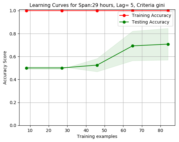
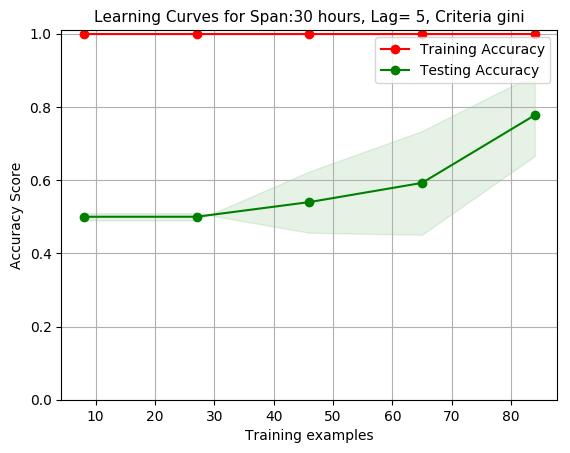
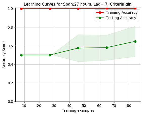
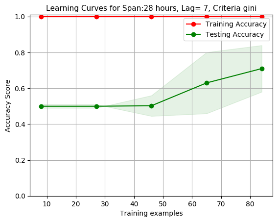
V-C Learning Curves
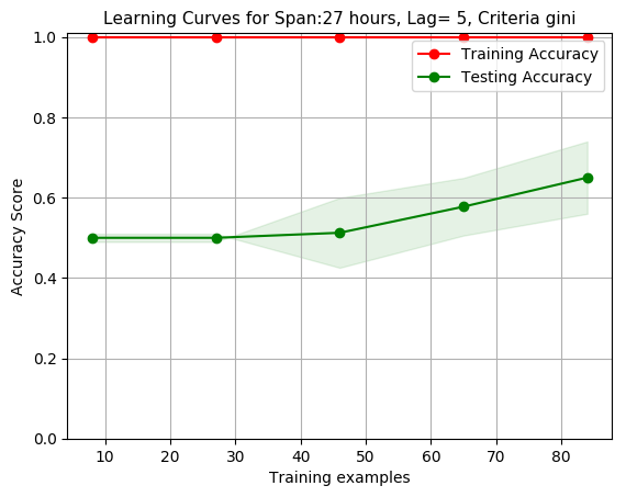
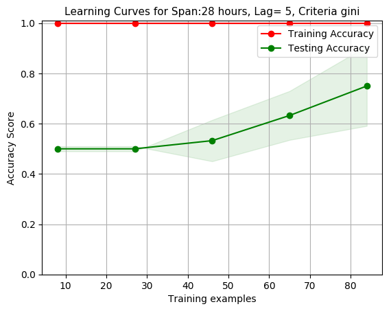
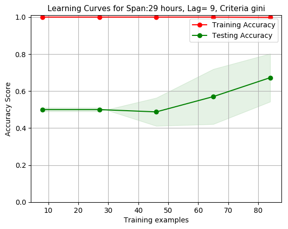
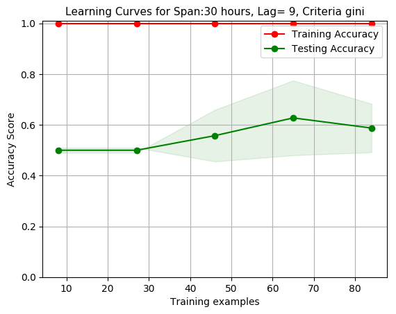
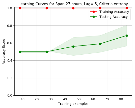
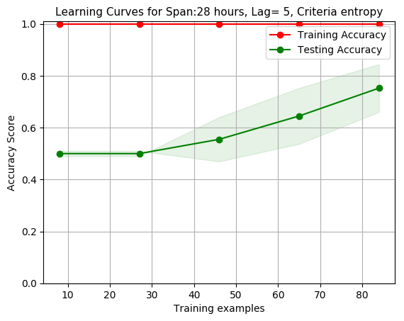
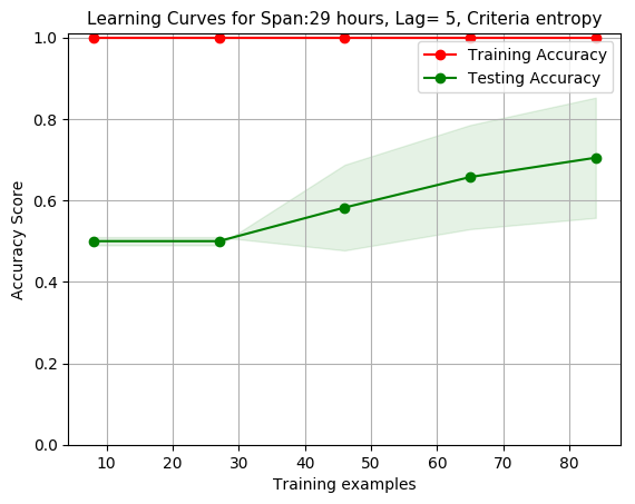
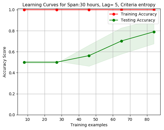
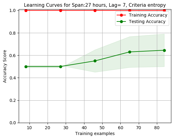
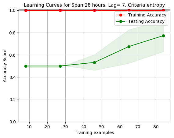
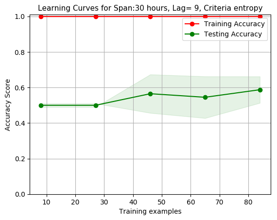
To be able to discriminate decision tree models that show similar accuracies we use the model learning curves, also called experience curves, to have an insight in how the accuracy changes as we feed the model with more training examples. Learning curves are particularly useful for comparing different algorithms [22] and choosing optimal model parameters during the design [23]. It is also a good tool for visually inspecting the sanity of the model in case of overtraining or undertraining. Figs. 6 and 7 show the learning curves of the decision tree model using gini and information gain as the splitting criteria respectively. The red line represents the training accuracy which evaluates the model on the newly trained data. The green line shows the testing accuracy which evaluates the model on the the never-seen testing data. The shaded area represents the standard deviation of the accuracies after running the model multiple times with the same number of training data. It is noticeable that the standard deviation becomes higher as the lag is increased. Also, it can be seen that the best average accuracies, that appeared in Fig. 5, are not always the ones that have the best learning curves. For example from Fig. 5, the best accuracy that has been reached appears to be in =7 and ; however, the learning curves corresponding to that span and lag show that the standard deviation is not very smooth as compared to =5. Therefore the experiments show that using =5 results in relatively stable models with lower variance. Therefore, we will zoom in =5 for all the spans that we previously filtered.
| Span 27 | Span 28 | Span 29 | Span 30 | |
|---|---|---|---|---|
|
Lag 5 |
 |
 |
 |
 |
|
Lag 7 |
 |
 |
 |
 |
|
Lag 9 |
 |
 |
 |
 |
| Span 27 | Span 28 | Span 29 | Span 30 | |
|---|---|---|---|---|
|
Lag 5 |
 |
 |
 |
 |
|
Lag 7 |
 |
 |
 |
 |
|
Lag 9 |
 |
 |
 |
 |
| Gini | Information Gain | |||||||
|---|---|---|---|---|---|---|---|---|
| Span | 27 | 28 | 29 | 30 | 27 | 28 | 29 | 30 |
| Accuracy | 0.64 | 0.74 | 0.73 | 0.74 | 0.77 | 0.70 | 0.67 | 0.78 |
| Recall | 0.69 | 0.70 | 0.74 | 0.70 | 0.76 | 0.70 | 0.70 | 0.73 |
| Precision | 0.62 | 0.75 | 0.75 | 0.76 | 0.78 | 0.72 | 0.72 | 0.86 |
| F1 | 0.65 | 0.75 | 0.75 | 0.74 | 0.79 | 0.71 | 0.69 | 0.82 |
| AUC | 0.65 | 0.72 | 0.74 | 0.73 | 0.76 | 0.70 | 0.69 | 0.77 |

To determine the best behaving model we choose six evaluation metrics that will assess the models’ performance from different aspects. Accuracy is the most standard evaluation measure used to assess the quality of a classifier by counting the ratio of correct classification over all the classifications. In this context the accuracy measure is particularly useful because our training and testing data is balanced. The data balance ensures that if the classifier is highly biased toward a given class it will be reflected on the accuracy measure. Recall is the second evaluation measure we considered, also known as the probability of detection, which characterizes the ability of the classifier to find all of the positive cases. Precision is used to evaluate the model with respect to the false alarms. In fact, precision is 1 - false alarm ratio. Precision and recall are usually anti-correlated; therefore, a useful quantity to compute is their harmonic mean, the F1 score. The last evaluation measure that we consider in the Area Under Curve (AUC) of the Receiver Operating Characteristic curve (ROC) curve. The intuition behind this measure is that AUC equals the probability that a randomly chosen positive example ranks above (is deemed to have a higher probability of being positive than) a randomly chosen negative example. It has been claimed in [24] that the AUC is statistically consistent and more discriminating than accuracy.
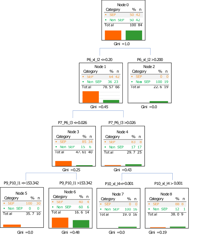
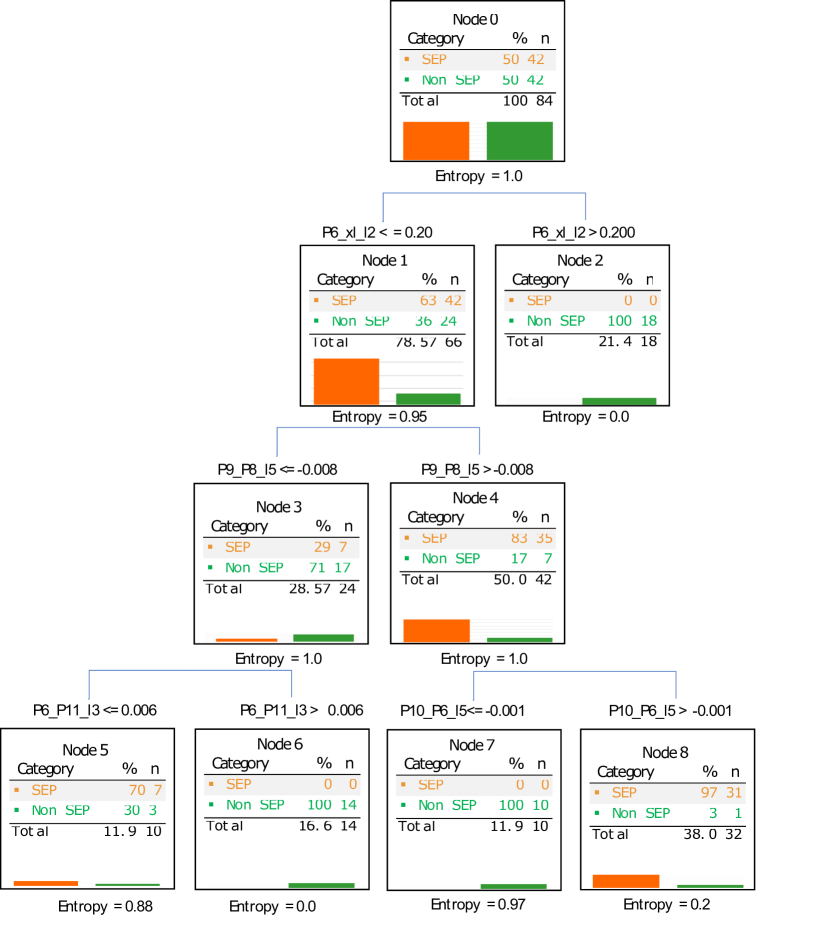
Table .IV shows the aforementioned evaluations on the =5 datasets. It is noticeable that span=30 achieves the best performance levels for both splitting criteria. The decision tree models corresponding to those settings using gini and information gain are shown in Fig. 9 and Fig. 10 respectively. For the purpose of visualization we used PCA dimensionality reduction technique to plot the full feature space with the 254 dimensions of the lag 5 and span 30 in Fig. 8-a, as well as the reduced feature space with only the selected features from the gini measure in Fig. 8-b and entropy measure in Fig. 8-c [25]. It is clearly visible that the SEP and non-SEP classes are almost indistinguishable when all the dimensions are used. When the decision tree feature selection is applied, the data points become more scattered in space and therefore easier for the classifier to distinguish. We also note that both decision tree classifiers have as a root a proton x-ray correlation parameter (). Some of the intermediate and leaf nodes have features that show correlations between proton channels is their conditions. This suggests that cross-correlations in proton channels are equally important to X-ray and proton channels correlations that appeared in [15]. Our best model shows a descent accuracy that is comparable (3% better) to the UMASEP system that uses the same catalog. We also made sure that our model is not biased towards the missing data of the lower energy channels P6 and P7 of GOES-12 by choosing the same number of samples of positive and negative class that happened during the GOES-12 coverage period.
VI Conclusion
In this paper we designed a new model to predict 100 MeV SEP events based on GOES satellite X-ray and proton data. This is the first effort that explores not only the dependencies between the X-ray and proton channels but also the auto-correlations and cross-correlations within the proton channels. We have found that proton channel cross-correlations based on a lag time (prior point in time) can be an important precursor as to whether an SEP event may happen or not. In particular, we started finding patterns starting from lag 5 and our best models shows both that the correlation between proton channel and X-ray channel is an important precursor to SEP events. Because of the missing data due to the failure of the P6 and P7 proton channels onboard GOES-12 we made sure that our dataset uses the same number of positive and negative examples coming from GOES-12. To our knowledge this is the first study that explores proton cross-channels correlations in order to predict SEP events. As a future extension of this study we are interested in doing ternary classification by further splitting the SEP class into impulsive and gradual. We are also interested in real-time SEP event predictions for practical applications of this research.
Acknowledgment
We thank all those involved with the GOES missions as well as the SOHO mission. We also acknowledge all the efforts of NOAA in making the catalogs and X-ray reports available. This work was supported in part by two NASA Grant Awards (No. NNX11AM13A, and No. NNX15AF39G), and one NSF Grant (No. AC1443061). The NSF Grant has been supported by funding from the Division of Advanced Cyberinfrastructure within the Directorate for Computer and Information Science and Engineering, the Division of Astronomical Sciences within the Directorate for Mathematical and Physical Sciences, and the Division of Atmospheric and Geospace Sciences within the Directorate for Geosciences.
References
- [1] A. Posner, “Up to 1-hour forecasting of radiation hazards from solar energetic ion events with relativistic electrons,” Space Weather, vol. 5, no. 5, 2007.
- [2] M. Desai and J. Giacalone, “Large gradual solar energetic particle events,” Living Reviews in Solar Physics, vol. 13, no. 1, p. 3, 2016.
- [3] “Space weather,” accessed on 11-21-2017. [Online]. Available: http://arcturan.com/space-weather/
- [4] S. Gabriel and J. Feynman, “Power-law distribution for solar energetic proton events,” Solar Physics, vol. 165, no. 2, pp. 337–346, 1996.
- [5] D. V. Reames, “Particle acceleration at the sun and in the heliosphere,” Space Science Reviews, vol. 90, no. 3-4, pp. 413–491, 1999.
- [6] J. Luhmann, S. Ledvina, D. Odstrcil, M. J. Owens, X.-P. Zhao, Y. Liu, and P. Riley, “Cone model-based SEP event calculations for applications to multipoint observations,” Advances in Space Research, vol. 46, no. 1, pp. 1–21, 2010.
- [7] J. B. Robinson, “Energy backcasting a proposed method of policy analysis,” Energy policy, vol. 10, no. 4, pp. 337–344, 1982.
- [8] A. Anastasiadis, A. Papaioannou, I. Sandberg, M. Georgoulis, K. Tziotziou, A. Kouloumvakos, and P. Jiggens, “Predicting flares and solar energetic particle events: The FORSPEF tool,” Solar Physics, vol. 292, no. 9, p. 134, 2017.
- [9] M. Dierckxsens, K. Tziotziou, S. Dalla, I. Patsou, M. Marsh, N. Crosby, O. Malandraki, and N. Lygeros, “The COMESEP SEP forecast tool,” in EGU General Assembly Conference Abstracts, vol. 16, 2014.
- [10] A. Aran, B. Sanahuja, and D. Lario, “Solpenco: A solar particle engineering code,” Advances in Space Research, vol. 37, no. 6, pp. 1240–1246, 2006.
- [11] S. Kahler, E. Cliver, and A. Ling, “Validating the proton prediction system (PPS),” Journal of atmospheric and solar-terrestrial physics, vol. 69, no. 1, pp. 43–49, 2007.
- [12] M. Laurenza, E. Cliver, J. Hewitt, M. Storini, A. Ling, C. Balch, and M. Kaiser, “A technique for short-term warning of solar energetic particle events based on flare location, flare size, and evidence of particle escape,” Space Weather, vol. 7, no. 4, 2009.
- [13] J. S. Neal and L. W. Townsend, “Predicting dose-time profiles of solar energetic particle events using bayesian forecasting methods,” IEEE transactions on nuclear science, vol. 48, no. 6, pp. 2004–2009, 2001.
- [14] M. Núñez, “Real-time prediction of the occurrence and intensity of the first hours of >100 MeV solar energetic proton events,” Space Weather, vol. 13, no. 11, pp. 807–819, 2015.
- [15] M. Nunez, “Predicting solar energetic proton events (E >10 MeV),” Space Weather, vol. 9, no. 7, 2011.
- [16] X. Xi, E. Keogh, C. Shelton, L. Wei, and C. A. Ratanamahatana, “Fast time series classification using numerosity reduction,” in Proceedings of the 23rd international conference on Machine learning. ACM, 2006, pp. 1033–1040.
- [17] J. D. Scargle, “Studies in astronomical time series analysis. ii-statistical aspects of spectral analysis of unevenly spaced data,” The Astrophysical Journal, vol. 263, pp. 835–853, 1982.
- [18] E. Zivot and J. Wang, “Vector autoregressive models for multivariate time series,” Modeling Financial Time Series with S-Plus®, pp. 385–429, 2006.
- [19] S. R. Safavian and D. Landgrebe, “A survey of decision tree classifier methodology,” IEEE transactions on systems, man, and cybernetics, vol. 21, no. 3, pp. 660–674, 1991.
- [20] W.-Y. Loh, “Classification and regression trees,” Wiley Interdisciplinary Reviews: Data Mining and Knowledge Discovery, vol. 1, no. 1, pp. 14–23, 2011.
- [21] D. Steinberg and P. Colla, “CART: classification and regression trees,” The top ten algorithms in data mining, vol. 9, p. 179, 2009.
- [22] P. Madhavan, “A new recurrent neural network learning algorithm for time series prediction,” Journal of Intelligent Systems, vol. 7, no. 1-2, pp. 103–116, 1997.
- [23] F. Pedregosa, G. Varoquaux, A. Gramfort, V. Michel, B. Thirion, O. Grisel, M. Blondel, P. Prettenhofer, R. Weiss, V. Dubourg et al., “Scikit-learn: Machine learning in python,” Journal of Machine Learning Research, vol. 12, no. Oct, pp. 2825–2830, 2011.
- [24] C. X. Ling, J. Huang, and H. Zhang, “AUC: a statistically consistent and more discriminating measure than accuracy,” in IJCAI, vol. 3, 2003, pp. 519–524.
- [25] S. Wold, K. Esbensen, and P. Geladi, “Principal component analysis,” Chemometrics and intelligent laboratory systems, vol. 2, no. 1-3, pp. 37–52, 1987.