An alternate approach to measure specific star formation rates at $2<z<7$

Abstract

We trace the specific star formation rate (sSFR) of massive star-forming galaxies ($\gtrsim\!10^{10}\,\mathcal{M}_{\odot}$) from $z\sim 2$ to 7. Our method is substantially different from previous analyses, as it does not rely on direct estimates of star formation rate, but on the differential evolution of the galaxy stellar mass function (SMF). We show the reliability of this approach by means of semi-analytical and hydrodynamical cosmological simulations. We then apply it to real data, using the SMFs derived in the COSMOS and CANDELS fields. We find that the $\mathrm{sSFR}$ is proportional to $(1+z)^{1.1\pm 0.2}$ at $z>2$, in agreement with other observations but in tension with the steeper evolution predicted by simulations from $z\sim 4$ to 2. We investigate the impact of several sources of observational bias, which however cannot account for this discrepancy. Although the SMF of high-redshift galaxies is still affected by significant errors, we show that future large-area surveys will substantially reduce them, making our method an effective tool to probe the massive end of the main sequence of star-forming galaxies.

1 Introduction

In less than 4 Gyr, between the Epoch of Reionization ($z\sim 8$) and the Cosmic Noon ($z\sim 2$), galaxies build almost half of the local universe’s stellar content (Madau & Dickinson, 2014). Key quantities to describe such a growth are galaxy stellar mass ($\mathcal{M}$) and star formation rate (SFR), whose ratio is the galaxy specific star formation rate ($\mathrm{sSFR}\equiv\mathrm{SFR}/\mathcal{M}$, i.e. the rate of mass doubling of a galaxy).

The sSFR of star-forming galaxies reflects their “main sequence” (MS) distribution (Noeske et al., 2007). Its evolution is a primary constraint both on processes that govern stellar mass accretion and the ones responsible for its cessation (the so-called “quenching” mechanisms). For instance, Renzini (2016) used analytical fits to sSFR($\mathcal{M},z$) and $\Psi(z)$ – the cosmic SFR density – to predict the galaxy quenching rate as a function of redshift (see also Peng et al., 2010; Boissier et al., 2010, for a similar approach). However this kind of analyses are still affected by significant uncertainties: at present there is no full concordance among the various sSFR measurements, especially at high redshift.

Figure 1 summarizes the state of the art in this context and highlights the substantial discrepancies in the measurements of the different studies. In this Figure, as well as in the rest of the paper, we refer to the sSFR$(z)$ computed at a constant stellar mass.

Pioneering studies at $z>3$ found a plateau in the sSFR evolution (e.g. Stark et al., 2009; Gonzalez et al., 2010), in tension with theoretical predictions (see Weinmann et al., 2011). In those papers $\mathcal{M}$ and SFR were derived by fitting their photometry with synthetic spectral energy distributions (SEDs) neglecting nebular emission contamination in the broad-band filters. This introduced a substantial bias in the sSFR estimates, as shown in Fig. 1 where a compilation of those studies (Behroozi et al., 2013b) is compared to more recent work. The latter, after accounting for optical emission lines in the SED fitting, find an increasing sSFR$(z)$ from $z=3$ to at least 7 (Stark et al., 2013; Gonzalez et al., 2014; de Barros et al., 2014). Another example of SED fitting systematics is shown in de Barros et al. (2014): their results change by an order of magnitude with varying assumption on star formation history (SFH), age, and metallicity. Moreover, when $\mathcal{M}$ and SFR are both derived through SED fitting, resulting biases are inter-connected and more difficult to correct.

Other studies use a different technique based on emission line contamination. They start from the color excess in broad-band filters to estimate H$\alpha$ equivalent width (EW), which is a good proxy for the sSFR. This novel approach does not rely on classical SED fitting recipes, even though it also makes use stellar population synthesis (SPS) models and needs assumptions on the SFH. Depending on the photometric baseline, it can yield results at $z=4\!-\!5$ (Shim et al., 2011; Rasappu et al., 2016) or over a larger redshift range ($1<z<6$, Faisst et al., 2016; Mármol-Quéralto et al., 2016).

Figure 1 marks other two caveats relevant for any sSFR estimator, namely the dust correction (see discussion in Pannella et al., 2015) and the observational biases (e.g. the Eddington bias, Eddington, 1913). Both have a significant impact especially at high redshift (Smit et al., 2014; Santini et al., 2017). Furthermore, diverging assumptions of the contamination of [NII] to H$\alpha$ affecting the SFR measurements from low-resolution spectroscopic surveys can lead to differences in the sSFR determinations (Faisst et al. in preparation). In addition, we note that – since the sSFR at fixed $z$ depends on stellar mass (e.g., Whitaker et al., 2014) – the scatter among the various estimates shown in Fig. 1 is also due to the fact that the sSFR is derived at different masses (between $5\times 10^{9}$ and $3\times 10^{10}\,\mathcal{M}_{\odot}$).

As a consequence, despite the improvements in observations, the sSFR($z$) function is still matter of debate. Several authors find an increase by a factor $\sim\!5$ across $3<z<7$ (e.g. Stark et al., 2013; de Barros et al., 2014; Salmon et al., 2015; Faisst et al., 2016) while others observe a flatter evolution (e.g. Gonzalez et al., 2014; Heinis et al., 2014; Tasca et al., 2015; Mármol-Quéralto et al., 2016). Different slopes imply discordant scenarios of galaxy evolution, with respect to gas accretion, stellar mass assembly, and quenching time-scales (Weinmann et al., 2011). Some discrepancy with simulations remains, especially at $1<z<3$ (e.g. Davé et al., 2016).

In this paper we provide a new sSFR constraint for star-forming galaxies up to $z\sim 7$, through a novel approach based on the evolution of their stellar mass function (SMF). Such a method, described in Sect. 2, offers a complementary point of view with respect to previous work. In fact, we rely on integrated quantities only (stellar mass and cumulative galaxy number density) without any direct SFR assessment. We demonstrate the validity of our approach by the use of cosmological simulations (Sect. 3) before applying the method to real data (Sect. 4). The results are discussed in Sect. 5 and then we conclude in Sect. 6.

We assume a $\Lambda$CDM cosmology with $\Omega_{\mathrm{m}}=0.3$, $\Omega_{\Lambda}=0.7$, and $H_{0}=70\,\mathrm{km}\,\mathrm{s}^{-1}\,\mathrm{Mpc}^{-1}$. The initial mass function (IMF) used as a reference is Chabrier (2003). We assume that the SMF shape is well described by a Schechter (1976) function, or a combination of two Schechter functions (with the same $\mathcal{M}_{\star}$ parameter) at $z<3$.

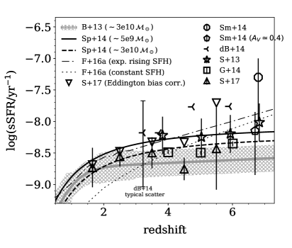
Figure 1: Estimates of sSFR($\mathcal{M},z$) from the literature, derived at $\mathcal{M}=5\!-\!30\times 10^{9}\,\mathcal{M}_{\odot}$ (depending on the study). The gray line with hatched area is the fit to data from studies published between 2007 and 2013 (Behroozi et al., 2013b). Another fit to the updated compilation of Speagle et al. (2014) is shown by a solid (dashed) line for sSFR at $\log(\mathcal{M/M}_{\odot})\simeq 9.7$ ($10.5$). Other symbols (see legend) show individual measurements from Stark et al. (2013), Gonzalez et al. (2014), de Barros et al. (2014), Smit et al. (2014, with different priors on dust extinction), Faisst et al. (2016, different star formation histories) and Santini et al. (2017, also including the Eddington bias correction). Not to compromise the readability of the figure, we show the error bar of only one point of de Barros et al. (2014); this is the 68% confidence limit derived from the whole probability distribution function of their SED models.

2 Method

2.1 Motivations

Before describing our method we highlight some of the main difficulties encountered in previous sSFR studies:

1. collecting a fully representative sample of star-forming galaxies, in a given mass range;

2. implementing realistic star formation histories in the SPS models;

3. defining physically motivated SED-fitting parameters and priors.

Limitations due to sample incompleteness are discussed e.g., in de Barros et al. (2014) and Speagle et al. (2014). Furthermore, recent work has reevaluated the fraction of star-forming galaxies at high-$z$ that are strongly enshrouded by dust (e.g. Casey et al., 2014; Mancini et al., 2015). This population may be missing in Lyman break galaxy (LBG) selections (see discussion in Capak et al., 2015). Argument ii) has a limited impact on stellar mass estimates (Santini et al., 2015) whereas the SFR is extremely sensitive to the SFH details (such as secondary bursts and star formation “frostings”). Concerning the third issue, examples of critical parameters are stellar metallicity, dust reddening, or the EW of nebular emission lines. Modifying their parametrization, or the range of allowed values, can produce significant differences both in $\mathcal{M}$ and SFR estimates (Conroy et al., 2009; Mitchell et al., 2013; Stefanon et al., 2015) as well as in their covariance matrix. The systematic effects inherited by the sSFR are discussed e.g. in Stark et al. (2013) and de Barros et al. (2014).

To circumvent these limitations as well as possible, we follow the semi-empirical approach described in Ilbert et al. (2013). The keystone of our method is the SMF of star-forming and quiescent galaxies. Their evolution from high ($z_{i}$) to low ($z_{f}<z_{i}$) redshift brings information on the stellar mass assembly (see also Wilkins et al., 2008). We perform our analysis in the COSMOS and CANDELS fields (Scoville et al., 2007 and Grogin et al., 2011) because their latest observations allows to probe the SMF with unprecedented accuracy and to higher redshifts.

2.2 Evolution of a single galaxy

The SMF evolution from $z_{i}$ (cosmic time $t_{i}$) to $z_{f}$ (i.e., $t_{f}>t_{i}$) can be modeled starting from the growth of individual galaxies. Broadly speaking, galaxy stellar mass accretion occurs through two channels: in situ star formation and galaxy merging. If we consider only the former process, the stellar mass of a galaxy at $z_{f}$ can be written as

$$\mathcal{M}(t_{f})=\mathcal{M}(t_{i})+\int_{t_{i}}^{t_{f}}\mathit{SFR}(t)\left[1-f_{\mathrm{return}}\right]\,\mathrm{d}t,$$ (1)

where the integral of the SFR accounts for the mass re-ejected into the interstellar medium via stellar winds and supernovae ($f_{\mathrm{return}}$). This can be taken as the instantaneous return fraction ($f_{\mathrm{return}}=0.43$ for a Chabrier IMF) or defined as a function of time as in Behroozi et al. (2013b):

$$f_{\mathrm{return}}=0.05\ln\left[1+\frac{t_{f}-t}{1.4\times 10^{6}\,\mathrm{yr}}\right].$$ (2)

One can simplify Eq. (1) by assuming that SFR($t$) is constant across $\Delta t\equiv t_{f}-t_{i}$. This is a fair approximation of the average SFH in the high-$z$ universe, at least on short time-scales like the $\Delta t$ steps that we consider (see below). A better fit may be a rising function, e.g. $\mathrm{SFR}\propto t^{\gamma}$ with $\gamma\sim 1.4\!-\!4$ (Papovich et al., 2011; Behroozi et al., 2013b). We discuss the implications of this choice in Section 3.2.

In addition, the fractional mass increase via mergers is

$$f_{\mathrm{merg}}=\int_{t_{i}}^{t_{f}}\frac{\dot{\mathcal{M}}_{\mathrm{merg}}}{\mathcal{M}(t_{i})}\,\mathrm{d}t=\int_{t_{i}}^{t_{f}}\frac{\mathcal{R}(t)}{\bar{\mu}}\,\mathrm{d}t,$$ (3)

where $\dot{\mathcal{M}}_{\mathrm{merg}}$ is the merger-driven stellar mass accretion rate, which can be written as a function of $\mathcal{R}$ (the merger rate) and $\bar{\mu}$ (the average stellar mass ratio between the target galaxy and the accreted satellite).

Equation (3) takes into account only the stellar mass already formed ex situ and accreted onto the given galaxy, neglecting possible bursts of star formation triggered by the galaxy-galaxy interaction. The latter is a well-established phenomenon in the local universe whereas it is less clear whether at higher redshift mergers can induce significant starburst episodes. In the standard hierarchical clustering scenario, the SFR enhancement per single merger is expected to increase with redshift as it is more likely that galaxy pairs have comparable mass (a condition for efficiently triggering starbursts, Cox et al., 2008); the fraction of destabilized gas is also larger at earlier epochs. However, recent hydrodynamical pc-resolution simulations (Fensch et al., 2017) show that such a large gas fraction (and gas clumpiness) does result in strong inflows and turbulence already in isolated objects, thus the interaction-induced star formation causes only a mild SFR increase (a factor $2\!-\!3$) over short timescales ($\sim\!50$ Myr). These findings are in agreement with other high-resolution prototypes of high-$z$ gas-rich mergers (Hopkins et al., 2013; Perret et al., 2014) but also with previous analyses (Cox et al., 2008). In another hydrodynamical simulation, this time with cosmological size, (Martin et al., 2017) find that the average enhancement due to either major or minor mergers is about 35% at $z\sim 3$. We also modify the model assuming $\times 2$ star formation increase (Robaina et al., 2009) over 100 Myr, finding negligible changes in our results. Therefore we decided not to include merger-driven starbursts in Equation (3).

We fix $\dot{\mathcal{M}}_{\mathrm{merg}}$ to be equal to $5\times 10^{9}\,\mathcal{M}_{\odot}\,\mathrm{Gyr}^{-1}$, according to Man et al. (2016). The authors derive this value for galaxies with $\log(\mathcal{M/M}_{\odot})>10.8$ at $0.5<z<2.5$ including both major and minor mergers, for which they observe $\mathcal{R}\sim 0.1\!-\!0.2$ and $\mathcal{R}\lesssim 0.1$ respectively. These values are also in good agreement with simulations (Hopkins et al., 2010). We extrapolate Man et al. results also at $z>2.5$ as they are consistent with the latest studies at higher redshift. For example observations in COSMOS and CANDELS indicate that for galaxies with $\mathcal{M}>10^{10}\,\mathcal{M}_{\odot}$ the major merger rate is $\mathcal{R}\leqslant 0.1\,\mathrm{Gyr}^{-1}$ up to $z\sim 3.5$, with an extrapolated trend towards higher $z$ that is nearly flat (Mundy et al., 2017, Duncan et al. in preparation). Observations with the Multi-Unit Spectroscopic Explorer (MUSE) in the Hubble Ultra Deep Field also find the same trend, with the major merger fraction that peaks at 20% at $z=2\!-\!3$ and then decreases towards $z=6$ (Ventou et al., 2017). Equation (3) will be re-tuned when additional data come out. We show the impact of the assumptions about $f_{\mathrm{return}}$ and $f_{\mathrm{merg}}$ in Section 3.2.

Eventually, with the approximation of constant SFR, the relation between the logarithmic increase $\Delta\log\!\mathcal{M}\equiv\log[\mathcal{M}(t_{f})/\mathcal{M}(t_{i})]$ and the galaxy sSFR is

$$\mathit{sSFR}(\mathcal{M}_{i},t_{i})=\frac{10^{\Delta\log\!\mathcal{M}}-1-f_{\mathrm{merg}}}{\Delta t-\int_{t_{i}}^{t_{f}}f_{\mathrm{return}}\,\mathrm{d}t},$$ (4)

where we define $\mathcal{M}_{i}\equiv\mathcal{M}(t_{i})$ for sake of clarity (i.e., the sSFR estimates we will show hereafter correspond to the initial redshift bin $z_{i}$). We note that $\Delta\log\!\mathcal{M}$ is the total stellar mass increase observed in a galaxy. To recover the net amount of stars formed in situ, and then the sSFR, this quantity must be corrected for mergers (Equation 3) and stellar mass loss (Equation 2) over the time interval $\Delta t$.

2.3 Matching sSFR($z$) to the SMF evolution

In order to apply Equation (4) one needs an estimate of $\Delta\log\!\mathcal{M}$. The formalism introduced in Section 2.2 describes the average growth in stellar mass, therefore we can look to the galaxy ensemble as encoded in the SMF. At a given stellar mass, we link star-forming galaxies at $z\sim z_{i}$ to their descendants at $z_{f}$ by tracking their cumulative number density ($\rho_{N}$, see van Dokkum et al., 2010; Behroozi et al., 2013a; Torrey et al., 2015). This is obtained from the integral of the star-forming SMF. However, some galaxies in the initial $z$-bin may quench their star formation before $z_{f}$. For this reason, the star-forming $\rho_{N}(>\mathcal{M}_{i})$ has to be corrected for the increased number density of quiescent galaxies (see Ilbert et al., 2013). Their fraction, as a function of $z$ and $\mathcal{M}$, can be derived from the quiescent SMF (inset in Figure 2, and also Figure 16 of Faisst et al., 2017b).

We connect galaxies at constant $\rho_{N}(>\mathcal{M}_{i})$ from $z_{i}$ to $z_{f}$ (van Dokkum et al., 2010). Figure 2 shows an example of such a procedure, using the SMFs observed in the COSMOS field at $z_{i}\simeq 3.25$ and $z_{f}\simeq 2.75$. Arrows in the figure show $\Delta\log\!\mathcal{M}$ for a constant $\rho_{N}(>\mathcal{M}_{i})$ evolution at different stellar masses. We choose $10^{10}<\mathcal{M}_{i}<10^{11}$, as this is the range where the SMF is well constrained by our data across the whole redshift range.

Then we repeat the procedure accounting for density evolution in the abundance matching. When connecting galaxies in the cumulative SMF to their descendants in the next $z$-bin, their $\mathcal{M}$ rank order may be different from the progenitors because of mergers and SFR scatter (e.g., Leja et al., 2013). In this case the merging events that must be taken into account are not only those involving a target galaxy (Section 2.2): the cumulative distribution is also modified by mergers between galaxies in lower mass bins that are promoted in the one for which we derive the sSFR. The SFR scatter also modifies the galaxy ranking in the abundance matching, as some low-mass galaxies can grow faster than others with higher mass. To correct the abundance matching for these effects we use the model provided by Torrey et al. (2015). The authors track the cumulative SMF at different epochs using the merger trees of the Illustris simulation (Genel et al., 2014; Vogelsberger et al., 2014a, b) and they fit the resulting number density evolution as a function of $z$ and $\mathcal{M}$. Following their recipe the $\rho_{N}$ threshold of galaxies at $t_{f}$ is slightly higher than their progenitors. However, as we will show in Section 3.1, this modification is a second-order effect that does not change any of our results (similarly to Salmon et al., 2015; Stefanon et al., 2017).

Concerning the issues listed in Section 2.1, we emphasize the following advantages of our method:

1. The SMF is corrected for incompleteness (in our case through the $1/V_{\mathrm{max}}$ method, Schmidt, 1968).

2. Even though the stellar mass of some peculiar galaxy class may strongly depend on the SFH (Michałowski et al., 2014), the SMF as a whole is much more stable against different configurations (Davidzon et al., 2013; Ilbert et al., 2013).

3. The sSFR we derive relies on a differential estimate ($\Delta\log\!\mathcal{M}$) and therefore systematic errors (e.g. due to SED fitting) are expected to cancel out.

This last argument holds unless the systematics vary rapidly as a function of redshift or galaxy type. A comparison with simulated galaxies suggests that this is not the case for our input dataset (Laigle et al. in preparation, see also Mitchell et al., 2013). The assumption of a universal IMF is an example of redshift-independent systematics in the SMF computation. For example, it produces a rigid offset of about $-0.24$ dex when converting from Salpeter (1955) to Chabrier (2003) IMF (e.g. Santini et al., 2015). Another systematic effect, namely the fixed metallicity range use in many SED fitting codes, is expect to vary slowly with redshift given the evolution of the mass-metallicity relation (Sommariva et al., 2012; Wuyts et al., 2016).

We also emphasize that whereas SMF measurements are usually corrected for the Malmquist (1922), this is rarely quantified in other analyses (e.g., those deriving the sSFR from the MS). The Eddington (1913) bias is another issue that SMF estimates usually take into account, although the correction technique is still uncertain (see discussion in Davidzon et al., 2017).

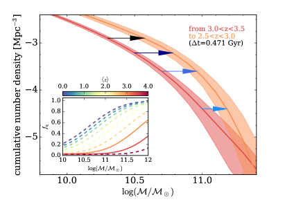
Figure 2: An example of abundance matching at constant cumulative galaxy number density, by integrating the star-forming SMFs measured in COSMOS2015 (from Davidzon et al., 2017) at $3<z<3.5$ and $2.5<z<3$ (red and orange line respectively, with shaded areas encompassing $1\sigma$ uncertainty). The four arrows trace the growth of galaxies that in the higher $z$-bin have $\mathcal{M}\sim 2$, 3, 5, and $10\times 10^{10}\,\mathcal{M}_{\odot}$. The number density of star-forming galaxies in the lower $z$-bin is corrected for recent quenching by removing the fraction of quiescent galaxy ($f_{\mathrm{q}}$). The $f_{\mathrm{q}}(\mathcal{M},z)$ evolution is shown in the inset, as it results from COSMOS2015 data (Bethermin et al., 2017, the two $z$-bins of interest are highlighted with solid lines).

3 Validation tests

In this Section we test whether the phenomenological model introduced above is a good description of the sSFR evolution. Tests are performed with a semi-analytical model (SAM, Section 3.1) and hydrodynamical simulations (Section 3.2). We quantify the impact of the various assumptions on which Equation (4) is based, e.g. the constant SFH. However, before showing the result of our tests, some premises must be clarified.

As the proposed method concerns star forming galaxies, we need to select them in the simulations. After a few experiments, we decided to use their intrinsic sSFR (hereafter sSFR₀) as provided by the theoretical model. In fact, a cut at $\log(\mathrm{sSFR}_{0}/\mathrm{yr}^{-1})>-11$ mimics the $NUV-r$ vs $r-J$ classification (NUVrJ) applied to the COSMOS data (Laigle et al., 2016). In real surveys, color-color diagrams are preferred to sSFR thresholds since rest-frame colors are more reliable (Conroy et al., 2009) and less SED-dependent (Davidzon et al., 2017). Theoretically the two classifications are very similar (Arnouts et al., 2013) so in the simulation we opted for a simpler sSFR cut. The paucity of quiescent galaxies at $z\gtrsim 3$ makes our results mostly insensitive at this caveat.

Since we want to verify that the framework we built is solid, we do not consider here additional uncertainties such as $z_{\mathrm{phot}}$ errors and sample incompleteness; moreover, the SMFs we will use in Section 4 have been corrected for this kind of observational biases. A thorough discussion about how to implement observational-like uncertainties in cosmological simulation will be addressed in Laigle et al. (in preparation).

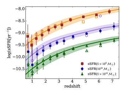
Figure 3: Evolution of the sSFR, for galaxies with $\mathcal{M}=5\!-\!50\times 10^{9}\,\mathcal{M}_{\odot}$ (see legend) in the Munich SAM (Henriques et al., 2015). Filled symbols represent the median of the sSFR($z$) in 20 light-cones (error bars being the standard deviation) derived from their SMF with a constant $\rho_{N}$ matching. Empty symbols show the results when we assume an evolving number density (as in Torrey et al., 2015). Solid lines are the median sSFR($z$) directly measured from the simulation in the same mass bins, with shaded areas enclosing 16th and 84th percentiles. The sSFR at $10^{10}$ and $5\times 10^{10}\,\mathcal{M}_{\odot}$ are shifted downward by 0.6 and 1.2 dex respectively, to improve readability.

3.1 Test with a semi-analytical model

We verify the reliability of out method by means of cosmological simulations. We choose the latest version of the Munich semi-analytical model (Henriques et al., 2015), based on the Millennium simulation, and select 20 independent light-cones with $1\deg$ diameter aperture to build mock galaxy catalogs similar to real data.

For each of these catalogs we estimate the star forming and passive SMFs in several bins of redshift, and trace the $\rho_{N}$ evolution as described in Section 2.3. We then apply Equation (4), setting $f_{\mathrm{return}}=0.43$ because this is the (instantaneous) mass loss fraction used in the SAM. As we will discuss below, this is a sensitive parameter in our method. For $f_{\mathrm{merg}}$ we use the observational values quoted in Section 2.2 after noticing that they are compatible with the merger rate of Millennium galaxies (Mundy et al., 2017).

We compare the sSFR($\mathcal{M}$,$z$) resulting from the SMF evolution with the median sSFR₀. The comparison for three distinct stellar mass bins is shown in Figure 3. Our method works well between $z\sim 2$ and $7$. We emphasize that with the abundance matching at constant $\rho_{N}$ we are able to accurately recover sSFR₀. Following the recipe of Torrey et al. (2015) the results do not change significantly, except at $z\gtrsim 5$ where their function produces an additional scatter (Figure 3). This is caused by the small-number statistics of massive halos hosting $\sim 10^{10}\,\mathcal{M}_{\odot}$ galaxies at $z\gtrsim 4$ (we find a similar behavior using the model of Behroozi et al., 2013a). For the same reason Torrey et al. (2015) focus their analysis below $z=3$, where the observed universe is more accurately reproduced by their hydrodynamical code. Supported by these tests, in the following we will link galaxy descendants at constant cumulative number density.

From the 20 light-cones of Henriques et al. we can provide a proxy for the cosmic variance expected in observations, since each light-cone has an area similar to the COSMOS field. The statistical error due to cosmic variance is always below $8\%$; this is the scatter in the median sSFR caused by field-to-field variations, not the error affecting the SMF (which propagates into the final outcome, see Section 5.1). At $z<1.5$ our estimates are less in agreement with sSFR₀, and with larger errors. This mainly depends on the fact that our model has been devised for the early universe. For instance the implemented galaxy merger rate is the one measured at $z\sim 2$, and also we did not model star formation quenching at the detailed level required at low $z$ (accounting for environmental effects that modify the SMF shape: Peng et al., 2010; Davidzon et al., 2016).

3.2 Testing systematic effects with an hydrodynamical model

We also test our method using the EAGLE simulation (Schaye et al., 2015). We take 10 snapshots (from $z=2.01$ to $z=5.97$) of a box with 100 Mpc side. We adopt the same configuration used in Section 2.1, but with the mass loss fraction parametrized as in Equation (2). In fact, EAGLE code assumes the same IMF of Henriques et al. (2015) but describes $f_{\mathrm{return}}$ more accurately, as a function of time and metallicity. However, SPS models show that $f_{\mathrm{return}}$ varies very little from $Z=0.004$ to solar metallicity thus Equation (2), which does not include metal enrichment, can be a reasonable approximation of their hydrodynamical model.

In this second test we quantify the systematic effects introduced by our method. Our “fiducial configuration” is the one that assumes constant $\mathrm{SFR}(t)$, $f_{\mathrm{return}}$ as in Equation (2), and includes stellar mass assembly via merging (Equation 3). Given that, we modify each of these parameters separately (Figure 4). To check if there is any $\mathcal{M}$-dependent bias, we perform this test in different mass bins up to $\log(\mathcal{M/M}_{\odot})=10.6$, as statistical fluctuation introduce too much noise beyond that threshold. Galaxy merging is the one with the smallest impact, as expected from the small value of $\dot{\mathcal{M}}_{\mathrm{merg}}$ and the short time interval between two $z$-bins. On the other hand, by replacing $f_{\mathrm{return}}(t)$ with a constant mass-loss fraction (equal to 0.43 for an IMF as in Chabrier, 2003) the sSFR increases by $0.10\!-\!0.15$ dex.

Systematics related to the SFH, which is kept constant in our fiducial set-up, are less straightforward to quantify because the choice of different parameterizations is not trivial. For instance, exponentially rising SFHs have been proposed as a suitable description of $z\sim 2$ galaxies (Maraston et al., 2010) although their rate of star formation ($\propto e^{t_{\mathrm{gal}}/\tau}$, where $t_{\mathrm{gal}}$ is the galaxy age) has been deemed too extreme (Pacifici et al., 2013; Salmon et al., 2015). This is especially true in our case, since the function in Equation (1) has to reproduce the average SFR. In agreement with Papovich et al. (2011) we opt for a power-law function, namely $\mathrm{SFR}\propto t_{\mathrm{gal}}^{1.5}$ (see also Salmon et al., 2015). This function needs an additional assumption on the time of galaxy formation: we parametrize it directly from simulations by fitting the $t_{\mathrm{gal}}$ distribution of $\sim\!10^{10}\,\mathcal{M}_{\odot}$ galaxies at different redshifts. When the SMF evolution is modeled assuming this power-law SFH, we obtain an sSFR slightly smaller than the fiducial estimate (Figure 4). This trend may be counterintuitive, but we remind that the sSFR is computed at the initial redshift $z_{i}$. Therefore, with a rising SFH, most of the stellar mass for a given $\Delta\log\mathcal{M}$ will form later. However, also with the modified SFR$(t)$, our results lie within $<\!30\%$ from sSFR₀ without a strong dependence on stellar mass. A better description of the average SFH should take into account a mix of different ages and the intrinsic SFR scatter among galaxies with similar mass. Such a refined characterization is beyond the aims of this paper.

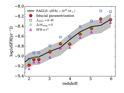
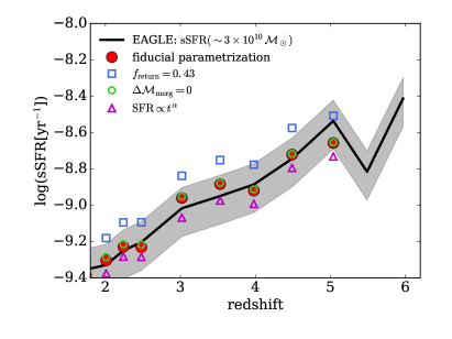
Figure 4: Systematic effects related to the main parameters of our method, tested with the EAGLE simulation (Schaye et al., 2015). In our “fiducial configuration” we assume a constant SFH with time-dependent $f_{\mathrm{return}}$, including the effect of galaxy mergers (see Sect. 2). The sSFR is computed at $10^{10}\,\mathcal{M}_{\odot}$ (upper panel) and $3\times 10^{10}\,\mathcal{M}_{\odot}$ (lower panel). At larger masses, this test is prevented by the low-number statistics in the simulated box. Both panels show how the results change if we consider: an instantaneous mass loss fraction $f_{\mathrm{return}}=0.43$ (blue squares), a negligible mass increase from mergers (green octagons), or a power-law rising SFH (magenta triangles, with $\alpha=1.5$). The solid line represents the intrinsic sSFR of EAGLE star-forming galaxies, with a gray shaded area that delimits $\pm 30$% variation.

4 Observational results

We apply our method (with the fiducial configuration) to the observed universe, taking data from Davidzon et al. (2017, hereafter D+17) and Grazian et al. (2015, hereafter G+15). The former measured the SMF from the COSMOS2015 galaxy catalog (Laigle et al., 2016) at $z\lesssim 6$ over 2 deg². G+15 provide an estimate of the SMF between $z=3.5$ and $7.5$, in three combined CANDELS fields (total area $368.90\,\mathrm{arcmin}^{2}$).

In both cases we consider their Schechter fits to the $1/V_{\mathrm{max}}$ points. We use the star-forming SMF of D+17 up to $z\sim 4$, where the distinction between star forming and passive galaxies is well determined by means of the NUVrJ diagram. In particular, we verify that a redshift-dependent NUVrJ cut evolves too slowly to have an impact on the results (Ilbert et al., 2015). In the star-forming SMF evolution we also have to account for the number density of newly quenched galaxies (see Section 2.3). For the COSMOS2015 sample, this correction factor is derived from the quiescent galaxy fraction ($f_{\mathrm{q}}$) and its growth with cosmic time. The $f_{\mathrm{q}}(\mathcal{M},z)$ function is analytically derived in Bethermin et al. (2017) using COSMOS2015 galaxies as a constraint (see their Equation 2) and is also shown in the inset of Figure 2. In CANDELS we work with the total mass function only, assuming that $f_{\mathrm{q}}$ is negligible at $z>4$. We do not connect the CANDELS $z\sim 4$ SMF to the COSMOS one at lower $z$, because of the different framework in which they were estimated.

Since we do not have access to the covariance matrix of G+15 Schechter fits, in the $\rho_{N}$ abundance matching we provide error bars derived from the Poisson uncertainty of CANDELS galaxy statistics (see Section 5.1). As mentioned above, we select the Schechter functions from G+15 and D+17 because they are corrected for the Eddington bias. We also try the SMF of the ZFOURGE survey (Tomczak et al., 2014, plot not shown), although the authors do not take this bias into account. Despite some scatter, ZFOURGE presents the same sSFR$(z)$ trend of COSMOS2015, suggesting that most of the Eddington bias may cancel out in our differential estimate (Straatman et al., 2016, or confirming that the medium-band imaging of ZFOURGE results in smaller $z_{\mathrm{phot}}$ and $\mathcal{M}$ errors).

We compute the sSFR($\mathcal{M},z$) at several fixed values of stellar mass (Table 1). Our results at $\log(\mathcal{M/M}_{\odot})\simeq 10.5$, close to the characteristic mass $\mathcal{M}_{\star}$, are shown in Figure 5. For sake of completeness we also include our estimates at $z<2$, despite the fact that the parameters of our method are calibrated for higher redshifts (Section 2.2); errors at such a low redshift are larger than $z=2\!-\!4$ mainly because $f_{\mathrm{q}}$ is higher, and its uncertainty significantly contributes to the total error budget. At $z>2$ we find a shallow sSFR evolution, proportional to $(1+z)^{1.1\pm 0.2}$. This trend is similar to what found in Gonzalez et al. (2014) and Tasca et al. (2015), while other sSFR estimates are higher in normalization (e.g. Heinis et al., 2014) or steeper in their redshift evolution (e.g., $\propto\!(1+z)^{1.5}$ in Faisst et al., 2016). However, the stellar mass range in one study may significantly differ from the others, making the comparison less straightforward especially if the linearity between $\log(\mathrm{SFR})$ and $\log(\mathcal{M})$ breaks up (Whitaker et al., 2014). To avoid confusion, in Figure 5 we show only analyses with median stellar masses comparable to ours (i.e., it does not exceed a factor $\sim\!3$ difference). We make an exception for studies at $z>4$, since none of them effectively probe $\mathcal{M}>10^{10}\,\mathcal{M}_{\odot}$ (Stark et al., 2013; Gonzalez et al., 2014; de Barros et al., 2014; Smit et al., 2016). This is indeed a distinctive feature of our method, which is effectively also in the highest-mass regime if the exponential tail of the SMF is sufficiently well constrained.

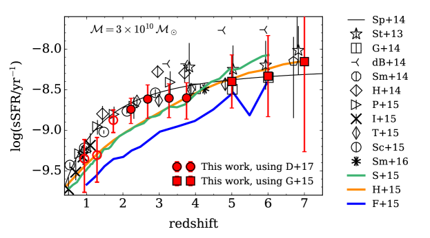
Figure 5: The sSFR at $3\times 10^{10}\,\mathcal{M}_{\odot}$ derived from the SMF evolution as observed in Davidzon et al. (2017, red circles) and Grazian et al. (2015, red squares). Although the method is optimized for $z>2$, we also show our results at lower redshifts (empty red circles). Estimates from Fig. 1 are reported here using the same symbols. In addition, we show the sSFR computed in Ilbert et al. (2015), Schreiber et al. (2015), Pannella et al. (2015), Tasca et al. (2015), Heinis et al. (2014), Smit et al. (2016). The black solid line is the Speagle et al. (2014) fitting function calculated at $3\times 10^{10}\,\mathcal{M}_{\odot}$. Blue, green, and orange lines show the sSFR($z$) from EAGLE, Illustris, and the latest Munich simulation respectively (Furlong et al., 2015; Sparre et al., 2015; Henriques et al., 2015).

5 Discussion

5.1 Selection effects and error budget

Despite consistent within $1\sigma$, our estimates are slightly below the “concordance” sSFR function resulting from the comprehensive review of Speagle et al. (2014). We argue that the offset can be ascribed to a different galaxy selection between our analysis and those in Speagle et al.: Using the NUVrJ diagram, our star-forming class includes also galaxies with moderate SFRs, which instead fall in the passive locus when using $U-V$ vs $V-J$ (UVJ, see discussion in Muzzin et al., 2013). On the other hand, several studies comprised in Speagle et al. may be biased towards bluer galaxies, due to their selection technique (e.g., LBG criteria) or because they intentionally focus on the core of the MS (e.g., by applying a $\sigma$-clipping to the distribution, Santini et al., 2017). Interestingly, the $z<1.4$ estimates from Ilbert et al. (2015), in which the SFRs are derived from UV-IR balance, also lie systematically below the concordance sSFR function. Based on a classification similar to ours, they are consistent with our trend (Figure 5).

Another potential problem is related to heavily dust-attenuated starburst galaxies, which may be missing in our sample. Thanks to the COSMOS2015 panchromatic detection strategy, which results in a high completeness of our sample, we conclude that such a bias is negligible (Laigle et al., 2016; D+17, ). This is confirmed by the good agreement with the sSFR of Schreiber et al. (2015), derived with a different technique (far-IR stacking of Herschel images) but also based on a mass-complete galaxy catalog. On the other hand, recent observations indicate that the dust content in high-$z$ galaxies varies over a wide range (e.g., Faisst et al., 2017a), which is a major concern for the SFR estimates based on rest-frame UV luminosity and has to be investigated in more detail with future far-IR measurements.

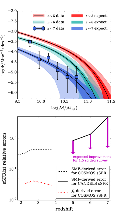
Figure 6: Upper panel: The SMF of CANDELS galaxies between $z=5$ and 7 black lines, from G+15. For each Schechter function, a transparent area shaded in light color encloses the $1\sigma$ uncertainty of the fit, calculated by taking into account Poisson noise only. At $z=7$, the $1/V_{\mathrm{max}}$ estimates are also plotted (blue squares). Opaque shaded areas (in darker colors) show the reduced statistical error that are expected for a CANDELS-like survey over 1.5 deg². Lower panel: Relative errors $\sigma_{\mathrm{sSFR}}/\mathrm{sSFR}$, with $\sigma_{\mathrm{sSFR}}$ corresponding to half the error bar of our estimates shown in Figure 5. At $z<4$ we decompose two sources of uncertainty: the error of the star-forming SMF (dashed line) and the one of the quiescent fraction used to correct for recently quenched galaxies (dot-dashed line, see Section 5.1). At $z>4$ only the former is considered (solid line). Arrows indicate the expected error reduction at $z>4$, if the SMF were constrained by a 1.5 deg² survey instead of the CANDELS data used in G+15.

For the sSFR derived from the D+17 SMF evolution, error bars include the $1\sigma$ uncertainty of the Schechter function along with the one of $f_{\mathrm{q}}(\mathcal{M},z)$. The former is the dominant source of uncertainty (Figure 6, bottom panel). The Schechter function in D+17 is a fit to the $1/V_{\mathrm{max}}$ determinations taking into account Poisson noise, cosmic variance, and the scatter due to SED fitting uncertainties. The resulting sSFR precision is comparable with the one of other studies, although some of them are reported in Figure 5 with the smaller errors derived e.g. from a stacking procedure, rather than the variance of the measurements. For instance, for Tasca et al. (2015) we plot the error on the median ($\sigma_{\mathrm{SFR}}/\sqrt{N}$) but the authors find $\sigma_{\mathrm{SFR}}=0.2\!-\!0.4$ dex when they consider the $\log(\mathrm{sSFR})$ dispersion. Error bars in Schreiber et al. (2015) are of the order of 0.1 dex but they do not include the effect of $z_{\mathrm{phot}}$ and $\mathcal{M}$ uncertainties (the authors also state $\sigma_{\mathrm{SFR}}=0.3$ dex).

At $z>4$ the SMF measurements become more uncertain, especially at $z\sim 7$, which is reflected in the sSFR. As noted in Section 4, G+15 provide only the marginalized $1\sigma$ error for each Schechter parameter. Without a covariance matrix, we approximate the $1\sigma$ error of the best-fit Schechter function deriving it from the Poisson statistics in the CANDELS volume (Figure 6, upper panel). Although in this way the SMF uncertainty is likely underestimated, the relative error $\sigma_{\mathrm{sSFR}}/\mathrm{sSFR}$ (Figure 6, bottom panel) is nonetheless large, up to a factor $\sim\!3$ at $z=7$. This illustrates the impact of small-number statistics in current high-$z$ surveys.

New observations over 1 deg², with resolution and depth similar to the CANDELS wide fields, should drastically reduce this issue. Combining them with existent CANDELS data, one would cover about $1.5$ deg², with the 1 deg² contiguous area probing cosmic structures over larger scales. In Figure 6 (upper panel) we show how the Poisson noise would decrease in the SMF of this hypothetical $1.5$ deg² galaxy survey, omitting the additional improvement in terms of cosmic variance. The expected gain in $\sigma_{\mathrm{sSFR}}/\mathrm{sSFR}$ is shown by arrows in the lower panel of the figure. We argue that the Hubble Space Telescope (HST) is the most suitable facility to achieve this goal. The James Webb Space Telescope (JWST) is not ideal for such a large-area survey, because overheads may reach $\sim\!80\%$ the exposure time (according to the JWST planning tool). Moreover, HST can provide parallel observations in optical bands, a unique benefit for supplementary $z<3$ studies. JWST instruments may then be used with a follow-up strategy, e.g. to better calibrate SED fitting estimates.

5.2 The massive end of the star-forming MS

The dependency of the SFR on stellar mass is also illustrated in Figure 7, where we multiplied sSFR$(\mathcal{M},z)$ by $\mathcal{M}$ to plot the star-forming MS at $\log(\mathcal{M/M}_{\odot})>10.2$. This is the mass threshold beyond which Whitaker et al. (2014) find a flattening of the $\mathrm{SFR}$-$\mathcal{M}$ relation at $z<2.5$ (see also Ilbert et al., 2015; Lee et al., 2015; Schreiber et al., 2015). Our $z<3$ data also suggest this trend. Figure 7 shows the MS we obtain at $z\sim 2.2$, along with the functional forms determined in Whitaker et al. (2014), Schreiber et al. (2015), and Tomczak et al. (2016). The difference among the three studies is mainly due to the way their samples are built.

A turnover mass is observed by (Tomczak et al., 2016) up to $z\sim 4$, although recently the ALMA Redshift 4 Survey has found opposite results (Schreiber et al., 2017). Besides them, other MS studies at high redshift probe a less massive regime: CANDELS (see Salmon et al., 2015) or the HST Frontier Field (HFF, Santini et al., 2017) do not have enough statistical power at $\log(\mathcal{M/M}_{\odot})>10.2$. For similar reasons, the high-mass end of the $z>4$ SMF is not well constrained and the MS we derive is highly uncertain. However, the SMF accuracy is easier to enhance than the statistics in SFR measurements, which require additional far-IR or sub-mm data. In this perspective, our method is expected to be an effective tool to constrain the massive end of the MS. At present, our analysis barely suggests that there is a flattening in the MS fit already at $z\sim 5$, while at higher redshift the relation $\mathrm{SFR}\propto\mathcal{M}^{\alpha}$ holds also for the most massive galaxies (with $\alpha$ close to unity as in the local universe, see Figure 7). If confirmed, this preliminary result will put fundamental constraints on the quenching time-scales of massive galaxies in the early universe, and their role during the epoch of reionization (cf. Sharma et al., 2016).

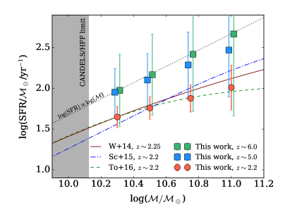
Figure 7: First constraints to the star-forming MS by using the sSFR$(\mathcal{M},z)$ derived from the SMF evolution. Estimates relying on D+17 are shown with filled circles, while squares indicated when the G+15 SMF is used (an horizontal offset of $\pm 0.015$ dex is applied to improve readability). Colored lines are not fits to the points, but the SFR$(\mathcal{M})$ functions calibrated in Whitaker et al. (2014, solid line), Schreiber et al. (2015, dot-dashed line), and Tomczak et al. (2016, dashed line) at the same redshift. A shaded area delimits the maximal stellar mass in other studies probing the MS at $z>3$ (Salmon et al., 2016; Santini et al., 2017).

5.3 Comparison to simulations

In Figure 5 we compare our results to state-of-the-art semi-analytical and hydrodynamical models (Sparre et al., 2015; Henriques et al., 2015; Furlong et al., 2015). These simulations suggest that the sSFR at $z<3$ is $\propto(1+z)^{2\!-\!2.5}$ as , while we find a shallower increase (with exponent $\sim 1.1$).

We first note that the slope is the same for the three simulations, although EAGLE has a lower normalization suggesting that the implemented stellar feedback could be too strong in its case (Furlong et al., 2015). This similarity is likely due to the fact that the star formation is tightly connected to the underlying dark matter accretion, irrespective of the different sub-grid baryon physics coded in the three simulations. To illustrate this point, in Figure 8 we contrast the sSFR of Illustris galaxies at $\log(\mathcal{M/M}_{\odot})\simeq 10.5$ to the specific dark matter accretion rate of their $\sim\!10^{12}\,\mathcal{M}_{\odot}$ hosting halos (see also Weinmann et al., 2011; Lilly et al., 2013).

Another reason for the discrepancy may be the presence of some selection effect. Previous comparisons between models and data have often classified galaxies through inconsistent criteria. For instance, Davé et al. (2016) extract from their $z>1$ simulation all the galaxies with $\log(\mathrm{sSFR/yr}^{-1})>-10.9$ and compare them to Whitaker et al. (2014), whose analysis based on the UVJ selection tends to exclude $\mathrm{sSFR\sim 10^{-10}\,\mathrm{yr}^{-1}}$ galaxies from the star-forming class (see D+17, ). We also mention Sparre et al. (2015), where the sSFR of all the Illustris galaxies in a given mass bin is compared to the sSFR function of Behroozi et al. (2013b), i.e. a fit to star-forming galaxies only. This choice however has no influence on their findings owing to the scarcity of massive quiescent galaxies in Illustris.

In our work the simulated star-forming sample is designed to be consistent to the observed one. The theoretical predictions shown in Figure 5 come from sSFR₀, i.e. the median of simulated galaxies after applying a cut at $\mathrm{sSFR}>10^{-11}\,\mathrm{yr}^{-1}$. This is a good proxy of the NUVrJ classification used in D+17. We also verify that neither a conservative cut at $10^{-9.5}\,\mathrm{yr}^{-1}$ can reconcile the lower sSFR in the simulations, implying that it is not caused by an excess of post-starburst galaxies (i.e., an over-populated “green valley” due to a too long quenching time-scale, Moutard et al., 2016).

Other observational biases that can impair the comparison are related to the way stellar mass and SFR are estimated. Hydrodynamical models usually define $\mathcal{M}$ as the sum of stellar particles gravitationally bounded to the galaxy sub-halo. This is an overestimate of the SED-fitting stellar mass, which is derived from aperture-corrected photometry and does not take into account the galaxy outskirt (i.e., the intra-cluster light). A value of sSFR closer to the observed one is obtained by considering only the inner 30 physical kpc of the given sub-halo (Schaye et al., 2015).

Regarding galaxy star formation, the instantaneous SFR should be replaced with an estimate averaged over the last $10\!-\!200$ Myr, i.e. the time-scales probed by the main SFR indicators (Sparre et al., 2017). Moreover, the SPS model used to build the SED templates may assume a stellar mass loss significantly different from the one of the simulation.

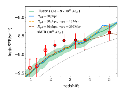
Figure 8: Comparison between our results (red symbols with error bars, as shown in Figure 5) and the sSFR predicted by Illustris at $3\times 10^{10}\,\mathcal{M}_{\odot}$. The solid green line and its shaded area are median sSFR and rms from Illustris, computed similarly to Sparre et al. (2015) but selecting only galaxies with $\mathrm{sSFR}>10^{-11}\,\mathrm{yr}^{-1}$. Furthermore, stellar mass and SFR of simulated galaxies have been progressively modified by considering: a galaxy radius ($R_{\mathrm{gal}}$) matching the one probed by aperture-corrected photometry (solid blue line) and the SFR over the last 10 or 250 Myr (dashed yellow and dot-dashed brown lines). The short-dashed gray line is the specific (dark) matter increase rate (sMIR, Neistein & Dekel, 2008) calculated for the average mass of the hosting halos as a function of redshift ($\sim\!10^{12}\,\mathcal{M}_{\odot}$).

To study the impact of these biases on our comparison, we modify the following properties of Illustris galaxies:

1. we re-compute $\mathcal{M}$ and SFR by including only stellar particles within 30 physical kpc from the galaxy center (the density peak of the sub-halo);

2. tracing backward the SFH of each particle, we calculate the SFR on two different time-scales: $\tau_{\mathrm{SFR}}=10$ and 250 Myr;

3. we modify each stellar particle by replacing their original return fraction with the one that follows Equation (2).

The outcomes of such a post-processing are summarized in Figure 8. The $f_{\mathrm{return}}$ modification (step 3) has a negligible impact and therefore is not included in the figure. This confirms our findings in Section 3.2, where we showed that Equation (2) is a good approximation of the return fraction implemented in the EAGLE code. The exclusion of the sub-halo outskirts (step 1) and the longer SFR time-scales (2) are not able to reconcile the $z<3$ theoretical predictions with our results. At higher redshifts a better agreement is reached when the sSFR of Illustris galaxies is calculated over the last 250 Myr, but the small-number statistics at $z>5$ prevent us from drawing strong conclusions.

If observational biases cannot account for the $z<3$ discrepancy, a solution should come from some improvement in the model’s physical prescriptions, likely concerning black-hole (BH) driven winds given the mass range we probe. In the “next generation” of Illustris (Illustris-TNG) both galactic winds and BH feedback are indeed modified (along with numerous other parameters, see Weinberger et al., 2017; Pillepich et al., 2017) and significant changes are expected especially for the sSFR of galaxies at $\log(\mathcal{M/M}_{\odot})>10.2$.

Table 1: Specific SFRs derived from the SMF evolution, for star-forming galaxies between $2\times 10^{10}$ and $10^{11}\,\mathcal{M}_{\odot}$ in different redshift bins. Null value is given in the range of stellar mass and redshift dominated by quiescent galaxies.

redshift	$\langle z\rangle^{\dagger}$	$\mathrm{\log(\mathrm{sSFR/yr}^{-1})}$
		at $\log(\mathcal{M/M}_{\odot})=10.3$	$\log(\mathcal{M/M}_{\odot})=10.5$	$\log(\mathcal{M/M}_{\odot})=10.7$	$\log(\mathcal{M/M}_{\odot})=11.0$
		using Davidzon et al. (2017) SMF:
$0.8<z\leqslant 1.1$	$0.94^{\ast}$	$-9.40^{+0.26}_{-0.49}$	$-9.33^{+0.23}_{-0.38}$	$-9.25^{+0.19}_{-0.28}$	$\dots$
$1.1<z\leqslant 1.5$	$1.29^{\ast}$	$-9.20^{+0.20}_{-0.28}$	$-9.29^{+0.21}_{-0.31}$	$-9.51^{+0.27}_{-0.61}$	$\dots$
$1.5<z\leqslant 2.0$	$1.74^{\ast}$	$-8.87^{+0.14}_{-0.16}$	$-8.87^{+0.12}_{-0.15}$	$-8.87^{+0.13}_{-0.15}$	$\dots$
$2.0<z\leqslant 2.5$	$2.22$	$-8.65^{+0.13}_{-0.15}$	$-8.74^{+0.14}_{-0.17}$	$-8.85^{+0.16}_{-0.20}$	$-8.99^{+0.27}_{-0.38}$
$2.5<z\leqslant 3.0$	$2.68$	$-8.59^{+0.18}_{-0.24}$	$-8.61^{+0.17}_{-0.24}$	$-8.70^{+0.20}_{-0.26}$	$-8.82^{+0.30}_{-0.41}$
$3.0<z\leqslant 3.5$	$3.27$	$-8.62^{+0.19}_{-0.24}$	$-8.60^{+0.17}_{-0.24}$	$-8.65^{+0.20}_{-0.25}$	$-8.84^{+0.35}_{-0.47}$
$3.5<z\leqslant 4.0$	$3.75$	$-8.56^{+0.16}_{-0.21}$	$-8.60^{+0.19}_{-0.26}$	$-8.64^{+0.24}_{-0.35}$	$-8.71^{+0.36}_{-0.62}$
		using Grazian et al. (2015) SMF:
$4.5<z\leqslant 5.5$	$5$	$-8.35^{+0.29}_{-0.37}$	$-8.40^{+0.32}_{-0.43}$	$-8.45^{+0.36}_{-0.53}$	$-8.53^{+0.47}_{-0.86}$
$5.5<z\leqslant 6.5$	$6$	$-8.32^{+0.43}_{-0.88}$	$-8.33^{+0.46}_{-1.07}$	$-8.34^{+0.51}_{-1.46}$	$-8.33^{+0.77}_{-2.58}$
$6.5<z\leqslant 7.5$	$7$	$-8.01^{+0.57}_{-0.81}$	$-8.15^{+0.91}_{-2.00}$	$-8.33^{+0.90}_{-2.44}$	$-8.69^{+0.97}_{-2.07}$

^†For D+17, $\langle z\rangle$ is the median $z_{\mathrm{phot}}$ of galaxies in the given $z$-bin; for G+15 it is the center of the bin. ^∗Estimates below the optimal redshift range of the method.

6 Conclusions

Thanks to deeper observations in the COSMOS and CANDELS fields, recent work has measured the $2<z<7$ SMF with unprecedented accuracy (Davidzon et al., 2017; Grazian et al., 2015). On this premise, we devised an advanced version of the semi-empirical technique described in Ilbert et al. (2013), to track the SMF evolution of star-forming galaxies and derive their median sSFR as a function of redshift. In contrast to other studies that require a direct measurement of the SFR, the fundamental ingredients here are $z_{\mathrm{phot}}$ and $\mathcal{M}$ estimates, along with a reliable technique (the NUVrJ diagram) to distinguish between star forming and passive galaxies. For this reason our method does not require expensive far-IR or sub-mm observations to derive SFRs, but only robust photometry in optical and near-IR bands. Moreover, issues like Malmquist and Eddington biases are routinely tackled in SMF analyses, while for other sSFR measurements it is more difficult to quantify their impact. However, we are limited to probing stellar masses $>\!10^{10}\,\mathcal{M}_{\odot}$ because the highest $z$-bins start to be incomplete below this threshold.

Using mock galaxy catalogs from cosmological simulations we demonstrated that our method works remarkably well from $z\sim 2$ up to $z\sim 7$. Most of the assumptions (e.g. related to SFH or galaxy merging) do not introduce significant systematics ($<\!30\%$). The parametrization of stellar mass loss must be carefully modeled, because a simplistic instantaneous return fraction can change the sSFR by $\sim\!0.1$ dex or more. The return fraction we assumed (Eq. 2) is in agreement with the one implemented in hydrodynamical simulations (EAGLE, Illustris).

Using the SMFs observed in COSMOS and CANDELS we found that $\mathrm{sSFR}\propto(1+z)^{1.1\pm 0.2}$ at $2<z<7$. At $z<4$ the trend of our data is in marginal tension with the theoretical expectation, even after correcting for the different $\mathcal{M}$ and SFR definitions (e.g., the time-scale over which the simulated SFR is calculated). This suggests a revision of the sub-grid physics in the models.

This work is preparatory to exploiting next-generation SMF estimates. At present, some of our findings are affected by the large uncertainties at $z>4$ (which are however of the same order of magnitude of other studies). One of these tentative results is the determination of the MS high-mass end from the observed sSFR$(z)$ up to $z\sim 6$, to identify the epoch when the linear relation between $\log(\mathrm{SFR})$ and $\log(\mathcal{M})$ starts to flatten. Future missions like Euclid or the Wide-Field Infrared Survey Telescope (WFIRST) will give the opportunity to significantly improve the galaxy SMF, especially by combining their data with the IR photometry from the Euclid/WFIRST Spitzer Legacy Survey (PI: P. Capak). Moreover, we have shown that if future HST observations covered a total area of $\geqslant\!1.5\,\mathrm{deg}^{2}$ with a depth similar to the CANDELS wide-fields, the statistical errors would dramatically reduce. Then, our technique shall provide unique constraints to the sSFR and MS evolution of massive galaxies.

References

- Arnouts et al. (2013) Arnouts, S., Le Floc’h, E., Chevallard, J., et al. 2013, A&A, 67, 1
- Behroozi et al. (2013a) Behroozi, P., Marchesini, D., Wechsler, R., et al. 2013a, ApJ, 777, L10
- Behroozi et al. (2013b) Behroozi, P. S., Wechsler, R. H., & Conroy, C. 2013b, ApJ, 770, 57
- Bethermin et al. (2017) Bethermin, M., Wu, H.-Y., Lagache, G., et al. 2017, A&A, in press, arXiv:1703.08795
- Boissier et al. (2010) Boissier., S., Buat, V., & Ilbert, O. 2010, A&A, 522, A18
- Capak et al. (2015) Capak, P. L., Carilli, C., Jones, G., et al. 2015, Nature, 522, 455
- Caputi et al. (2017) Caputi, K. I., Deshmukh, S., Ashby, M. L. N., et al. 2017, ApJ, 849, 45
- Casey et al. (2014) Casey, C. M., Narayanan, D., & Cooray, A. 2014, Physics Reports, 541, 45
- Chabrier (2003) Chabrier, G. 2003, PASP, 115, 763
- Conroy et al. (2009) Conroy, C., Gunn, J., & White, M. 2009, ApJ, 699, 486
- Cox et al. (2008) Cox, T. J., Jonsson, P., Somerville, R. S., Primack, J. R., & Dekel, A. 2008, MNRAS, 384, 386
- Davé et al. (2016) Davé, R., Thompson, R. J., & Hopkins, P. F. 2016, MNRAS, 462, 3265
- Davidzon et al. (2013) Davidzon, I., Bolzonella, M., Coupon, J., et al. 2013, A&A, 558, A23
- Davidzon et al. (2016) Davidzon, I., Cucciati, O., Bolzonella, M., et al. 2016, A&A, 586, A23
- Davidzon et al. (2017) Davidzon, I., Ilbert, O., Laigle, C., et al. 2017, A&A, in press, arXiv:1701.02734
- de Barros et al. (2014) de Barros, S., Schaerer, D., & Stark, D. 2014, A&A, 563, A81
- Eddington (1913) Eddington, A. 1913, MNRAS, 73, 359
- Faisst et al. (2016) Faisst, A. L., Capak, P., Hsieh, B. C., et al. 2016, ApJ, 821, 122
- Faisst et al. (2017a) Faisst, A. L., Capak, P., Yan L., et al. 2017a, ApJ, in press, arXiv:1708.07842
- Faisst et al. (2017b) Faisst, A. L., Carollo, C., Capak, P., et al. 2017b, ApJ, 839, 71
- Fensch et al. (2017) Fensch, J., Renaud, F., Bournaud, F., et al. 2017, MNRAS, 465, 1934
- Furlong et al. (2015) Furlong, M., Bower, R. G., Theuns, T., et al. 2015, MNRAS, 450, 4486
- Genel et al. (2014) Genel, S., Vogelsberger, M., Springel, V., et al. 2014, MNRAS, 445, 175
- Gonzalez et al. (2014) Gonzalez, V., Bouwens, R., Llingworth, G., et al. 2014, ApJ, 781, 34
- Gonzalez et al. (2010) Gonzalez, V., Labbe, I., Bouwens, R. J., et al. 2010, ApJ, 713, 115
- Grazian et al. (2015) Grazian, A., Fontana, A., Santini, P., et al. 2015, A&A, 575, A96
- Grogin et al. (2011) Grogin, N., Kocevski, D., Faber, S., et al. 2011, ApJS, 197, 35
- Heinis et al. (2014) Heinis, S., Buat, V., Béthermin, M., et al. 2014, MNRAS, 437, 1268-1283
- Henriques et al. (2015) Henriques, B., White, S., Thomas, P., et al. 2015, MNRAS, 451, 2663
- Hopkins et al. (2010) Hopkins, P. F., Bundy, K., Croton, D., et al. 2010, ApJ, 715, 202
- Hopkins et al. (2013) Hopkins, P. F., Cox, T. J., Hernquist, L., et al. 2013, MNRAS, 430, 1901
- Ilbert et al. (2013) Ilbert, O., McCracken, H. J., Le Fèvre, O., et al. 2013, A&A, 556, A55
- Ilbert et al. (2015) Ilbert, O., Arnouts, S., Floc’h, E. L., et al. 2015, A&A, 579, A2
- Kaviraj et al. (2013) Kaviraj, S., Cohen, S., Windhorst, R. A., et al. 2013, MNRAS, 429, L40
- Laigle et al. (2016) Laigle, C., McCracken, H., Ilbert, O., et al. 2016, ApJ, 224, 24
- Leja et al. (2013) Leja, J., van Dokkum, P., & Franx, M. 2013, ApJ, 766, 33
- Lee et al. (2015) Lee, N., Sanders, D. B., Casey, C. M., et al. 2015, ApJ, 801, 80
- Lilly et al. (2013) Lilly, S. J., Carollo, C. M., Pipino, A., Renzini, A., & Peng, Y. 2013, ApJ, 772, 119
- Lotz et al. (2010) Lotz, J. M., Jonsson, P., Cox, T. J., & Primack, J. R. 2010, MNRAS, 404, 575
- Madau & Dickinson (2014) Madau, P., & Dickinson, M. 2014, ARA&A, 52, 415
- Malmquist (1922) Malmquist, K. G., 1922, Meddelanden fran Lunds Astronomiska Observatorium Serie I, 100, 1
- Man et al. (2016) Man, A. W. S., Zirm, A. W., & Toft, S. 2016, ApJ, 830, 89
- Mancini et al. (2015) Mancini, M., Schneider, R., Graziani, L., et al. 2015, MNRAS, 451, L70
- Maraston et al. (2010) Maraston, C., Pforr, J., Renzini, A., et al. 2010, MNRAS, 407, 830
- Mármol-Quéralto et al. (2016) Mármol-Quéralto, E., McLure, R. J., Cullen, F., et al. 2016, MNRAS, 460, 3587
- Martin et al. (2017) Martin, G., Kaviraj, S., Devriendt, J. E. G., et al. 2017, MNRAS, 472, L50
- Michałowski et al. (2014) Michałowski, M. J., Hayward, C. C., Dunlop, J. S., et al. 2014, ArXiv e-prints
- Mitchell et al. (2013) Mitchell, P. D., Lacey, C. G., Baugh, C. M., & Cole, S. 2013, MNRAS, 435, 87
- Moutard et al. (2016) Moutard, T., Arnouts, S., Ilbert, O., et al. 2016, A&A, 590, A103
- Mundy et al. (2017) Mundy, C. J., Conselice, C. J., Duncan, K. J., et al. 2017, MNRAS, accepted, arXiv:1705.07986
- Muzzin et al. (2013) Muzzin, A., Marchesini, D., Stefanon, M., et al. 2013, ApJ, 777, 18
- Neistein & Dekel (2008) Neistein, E., & Dekel, A. 2008, MNRAS, 383, 615
- Noeske et al. (2007) Noeske, K., Weiner, B., Faber, S., et al. 2007, ApJ, 660, L43
- Pacifici et al. (2013) Pacifici, C., Kassin, S. A., Weiner, B., Charlot, S., & Gardner, J. P. 2013, ApJ, 762, L15
- Pannella et al. (2015) Pannella, M., Elbaz, D., Daddi, E., et al. 2015, ApJ, 807, 141
- Papovich et al. (2011) Papovich, C., Finkelstein, S. L., Ferguson, H. C., Lotz, J. M., & Giavalisco, M. 2011, MNRAS, 412, 1123
- Peng et al. (2010) Peng, Y.-j., Lilly, S., Kovač, K., et al. 2010, ApJ, 721, 193
- Perret et al. (2014) Perret, V., Renaud, F., Epinat, B., et al. 2014, A&A, 562, A1
- Pillepich et al. (2017) Pillepich, A., Springel, V., Nelson, D., et al. 2017, MNRAS, submitted, eprint arXiv:1703.02970
- Planck Collaboration (2014) Planck Collaboration, P., Ade, P. A. R., Aghanim, N., et al. 2014, A&A, 571, A16
- Rasappu et al. (2016) Rasappu, N., Smit, R., Labbe, I., et al. 2016, MNRAS, 461, 3886
- Renzini (2016) Renzini, A. 2016, 6
- Robaina et al. (2009) Robaina, A. R., Bell, E. F., Skelton, R. E., et al. 2009, ApJ, 704, 324
- Rodighiero et al. (2011) Rodighiero, G., Daddi, E., Baronchelli, I., et al. 2011, ApJ, 739, L40
- Rodriguez-Gomez et al. (2015) Rodriguez-Gomez, V., Genel, S., Vogelsberger, M., et al. 2015, MNRAS, 449, 49
- Salmon et al. (2015) Salmon, B., Papovich, C., Finkelstein, S. L., et al. 2015, ApJ, 799, 183
- Salmon et al. (2016) Salmon, B., Papovich, C., Long, J., et al. 2016, 18
- Salpeter (1955) Salpeter, E. 1955, ApJ, 121, 161
- Santini et al. (2015) Santini, P., Ferguson, H. C., Fontana, A., et al. 2015, ApJ, 801, 97
- Santini et al. (2017) Santini, P., Fontana, A., Castellano, M., et al. 2017, ApJ, submitted, eprint arXiv:1706.07059
- Schaye et al. (2015) Schaye, J., Crain, R. A., Bower, R. G., et al. 2015, MNRAS, 446, 521
- Schreiber et al. (2015) Schreiber, C., Pannella, M., Elbaz, D., et al. 2015, A&A, 575, A74
- Schreiber et al. (2017) Schreiber, C., Pannella, M., Leiton, R., et al. 2017, A&A, 599, A134
- Schechter (1976) Schechter, P. 1976, ApJ, 203, 297
- Schmidt (1968) Schmidt, M. 1968, ApJ, 151, 393
- Scoville et al. (2007) Scoville, N., Aussel, H., Brusa, M., et al. 2007, ApJS, 172, 1
- Sharma et al. (2016) Sharma, M., Theuns, T., Frenk, C., et al. 2016, MNRAS, 458, L94
- Shim et al. (2011) Shim, H., Chary, R.-R., Dickinson, M., et al. 2011, ApJ, 738, 69
- Smit et al. (2014) Smit, R., Bouwens, R. J., Labbe, I., et al. 2014, ApJ, 784, 58
- Smit et al. (2016) Smit, R., Bouwens, R., Labbé, I., et al. 2016, ApJ, 833, 254
- Sommariva et al. (2012) Sommariva, V., Mannucci, F., Cresci, G., et al. 2012, A&A, 539, A136
- Sparre et al. (2017) Sparre, M., Hayward, C. C., Feldmann, R., et al. 2017, MNRAS, 466, 88
- Sparre et al. (2015) Sparre, M., Hayward, C., Springel, V., et al. 2015, MNRAS, 447, 3548
- Speagle et al. (2014) Speagle, J. S., Steinhardt, C. L., Capak, P. L., & Silverman, J. D. 2014, ApJS, 214, 15
- Stark et al. (2009) Stark, D. P., Ellis, R. S., Bunker, A., et al. 2009, ApJ, 697, 1493
- Stark et al. (2013) Stark, D. P., Schenker, M. A., Ellis, R., et al. 2013, ApJ, 763, 129
- Stefanon et al. (2017) Stefanon, M., Bouwens, R. J., Labbé, I., et al. 2017, ApJ, 843, 36
- Stefanon et al. (2015) Stefanon, M., Marchesini, D., Muzzin, A., et al. 2015, ApJ, 803, 23
- Straatman et al. (2016) Straatman, C. M. S., Spitler, L. R., Quadri, R. F., et al. 2016, ApJ, 830, 51
- Tasca et al. (2015) Tasca, L. A. M., Le Fèvre, O., Hathi, N. P., et al. 2015, A&A, 581, A54
- Tomczak et al. (2014) Tomczak, A. R., Quadri, R. F., Tran, K.-V. H., et al. 2014, ApJ, 783, 85
- Tomczak et al. (2016) —. 2016, ApJ, 817, 16
- Torrey et al. (2015) Torrey, P., Wellons, S., Machado, F., et al. 2015, MNRAS, 454, 2770
- van Dokkum et al. (2010) van Dokkum, P. G., Whitaker, K. E., Brammer, G., et al. 2010, ApJ, 709, 1018
- Ventou et al. (2017) Ventou, E., Contini, T., Bouché, N., et al. 2017, arXiv:1711.00423
- Vogelsberger et al. (2014a) Vogelsberger, M., Genel, S., Springel, V., et al. 2014a, Nature, 509, 177-182
- Vogelsberger et al. (2014b) Vogelsberger, M., Genel, S., Springel, V., et al. 2014b, MNRAS, 444, 1518-1547
- Weinberger et al. (2017) Weinberger, R., Springel, V., Hernquist, L., et al. 2017, MNRAS, 465, 3291
- Weinmann et al. (2011) Weinmann, S. M., Neistein, E., & Dekel, A. 2011, MNRAS, 417, 2737
- Whitaker et al. (2014) Whitaker, K. E., Franx, M., Leja, J., et al. 2014, ApJ, 795, 104
- Wilkins et al. (2008) Wilkins, S. M., Trentham, N., & Hopkins, A. M. 2008, MNRAS, 385, 687
- Wuyts et al. (2016) Wuyts, E., Wisnioski, E., Fossati, M., et al. 2016, ApJ, 827, 74
- Xu et al. (2012) Xu, C. K., Zhao, Y., Scoville, N., et al. 2012, ApJ, 747, 85