Solving the puzzle of discrepant quasar variability on monthly time-scales implied by SDSS and CRTS data sets

Abstract

We present an improved photometric error analysis for the 7,100 CRTS (Catalina Real-Time Transient Survey) optical light curves for quasars from the SDSS (Sloan Digital Sky Survey) Stripe 82 catalogue. The SDSS imaging survey has provided a time-resolved photometric data set which greatly improved our understanding of the quasar optical continuum variability: Data for monthly and longer time-scales are consistent with a damped random walk (DRW). Recently, newer data obtained by CRTS provided puzzling evidence for enhanced variability, compared to SDSS results, on monthly time-scales. Quantitatively, SDSS results predict about 0.06 mag root-mean-square (rms) variability for monthly time-scales, while CRTS data show about a factor of 2 larger rms, for spectroscopically confirmed SDSS quasars. Our analysis has successfully resolved this discrepancy as due to slightly underestimated photometric uncertainties from the CRTS image processing pipelines. As a result, the correction for observational noise is too small and the implied quasar variability is too large. The CRTS photometric error correction factors, derived from detailed analysis of non-variable SDSS standard stars that were re-observed by CRTS, are about 20-30%, and result in reconciling quasar variability behaviour implied by the CRTS data with earlier SDSS results. An additional analysis based on independent light curve data for the same objects obtained by the Palomar Transient Factory provides further support for this conclusion. In summary, the quasar variability constraints on weekly and monthly time-scales from SDSS, CRTS and PTF surveys are mutually compatible, as well as consistent with DRW model.

1 Introduction

Variability can be used to both select and characterize quasars in sky surveys (for a recent overview see Lawrence 2016). Although various time-scales of variability can be linked to physical parameters, such as accretion disc viscosity, or corona geometry (Kelly et al. 2011; Graham et al. 2014), the physical mechanism remains elusive. Most viable explanations for observed variability include accretion disc instabilities (Kawaguchi et al., 1998), surface thermal fluctuations from magnetic field turbulence (Kelly et al., 2009), and coronal X-ray heating (Kelly et al., 2011, see Kozłowski 2016 for a review).

The diversity of physical scenarios available to explain the origin of quasar variability results in a variety of ways to characterize it. The two most widely used approaches to describing the variability of quasars include a structure function (SF) analysis and light curve fitting based on damped random walk (DRW, also known as the Ornstein–Uhlenbeck process) model (Kelly et al. 2007; MacLeod et al. 2011). An SF analysis essentially measures the width of the magnitude difference distribution as a function of the time separation, $\Delta t$. The DRW model approach is better suited for well-sampled light curves with a typical cadence of days (Zu et al., 2013; Kozłowski, 2016), whereas an ensemble SF analysis is better for sparsely sampled light curves (Hawkins, 2002; Vanden Berk et al., 2004; de Vries et al., 2005); for a review and discussion see Kozłowski (2016). Although the sampling for CRTS (the Catalina Real-time Transient Survey) light curves analysed here (see Section 2.2) might be adequate for light curve fitting, we nevertheless opt for the SF approach because it allows for more straightforward analysis when data quality is suspect.

The observed SF is often characterized by a simple power law (Schmidt et al., 2010). If the probed time-scales are long enough ($\sim$ years), the power law flattens above a characteristic tim-scale, $\tau$ (Ivezić et al., 2004; Kelly et al., 2007; MacLeod et al., 2010). This time-scale may correspond to a transition from the stochastic thermal process that drives the variability to the physical response of the disc that successfully dampens the amplitude on longer time-scales (Collier & Peterson, 2001; Kelly et al., 2007; Kelly et al., 2009; Kelly et al., 2011; Lawrence, 2016). In the context of a DRW model, the expected SF is described by

$${\rm SF}(\Delta t)={\rm SF}_{\infty}\,\left[1-\exp(-\Delta t/\tau)\right]^{1/2},$$ (1)

where ${\rm SF}_{\infty}$ is the asymptotic value of the SF (for $\Delta t\ll\tau$, SF($\Delta t$) $\propto\Delta t^{1/2}$).

Most studies found that $\tau>100$ d (MacLeod et al. 2010; Kozłowski 2016). It is a relatively short time-scale compared to the dominant time-scale of variation for quasars, that exceeds 10 years (Hawkins, 2007). Recently, Graham et al. (2014) found a characteristic time-scale in quasar’s rest frame of about 54 d, using the Slepian wavelet variance (SWV) analysis of CRTS light curves (the SWV time-scale denotes the point at which the ensemble SWV for quasars deviates from the ensemble SWV for a DRW realization of the same data set, and is thus different from $\tau$ obtained in DRW analysis). This short time-scale implies much stronger variability on monthly time-scales than observed in SDSS data: SDSS results from MacLeod et al. (2010) predict about 0.06 mag root-mean-square (rms) variability for time-scales below 50 d, while this CRTS-based analysis implies about a factor of 2 larger rms. These discrepancies have serious implications for physical interpretations of quasar variability: Observed time-scales are directly related to physical processes and increased variability levels call in question DRW as a viable model for describing quasar light curves (MacLeod et al. 2010; Kozłowski 2016).

It is not obvious whether these discrepancies are due to various problems with the CRTS and/or SDSS data sets (inadequate sampling, incorrect estimates of photometric errors, etc.), or perhaps are due to different analysis methods (SWV versus SF analysis). Here, we reanalyse these CRTS data using the same SF method as used by MacLeod et al. (2010) to analyse SDSS data, and investigate the origin of these discrepant time-scales and variability levels. We argue that the most likely explanation of these discrepancies are slightly under-estimated photometric errors for CRTS light-curve data.

2 Data Sets

We study stars and quasars selected from the sky region known as SDSS Stripe 82 (S82; an $\sim$300 deg² large region along the celestial equator: $22^{h}24^{m}<\mathrm{RA}<04^{h}08^{m}$ and $\mathrm{|Dec|}<1.27^{\circ}$). We utilize both SDSS and CRTS photometric data.

2.1 Sloan Digital Sky Survey (SDSS)

We use two SDSS catalogues, with five-band near-simultaneous photometry for 9258 quasars, and 1 006 849 standard stars (non-variable stars, as implied by the repeated SDSS photometry, see Ivezić et al. 2007). The quasar catalogue includes spectroscopically confirmed quasars from the SDSS Data Release 7 (Abazajian et al., 2009), based on the SDSS Quasar Catalogue V (Schneider et al., 2010), and was compiled by MacLeod et al. (2012). The SDSS standard stars catalogue was constructed as described in Ivezić et al. (2007).

2.2 Catalina Real-time Transient Survey (CRTS)

The main goal of CRTS was to find near-Earth objects. Its short intra-night cadence (four exposures per night) was designed to allow a rapid follow-up (Graham et al., 2015), and white light (without filter) light curves maximize the sensitivity for faint objects. Three survey telescopes (the 0.7 m Catalina Sky Survey Schmidt in Arizona, the 1.5 m Mount Lemmon Survey telescope in Arizona, and the 0.5 m Siding Spring Survey Schmidt in Australia) were equipped with identical, 4kx4k CCDs (see Djorgovski et al. 2011 for technical details). Although, in principle, white light magnitudes can be calibrated to Johnson’s V-band zero-point (Drake et al., 2013), this step was unnecessary in our analysis.

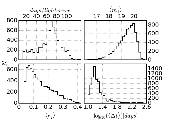
In this study, we used a sample of 7932 spectroscopically confirmed S82 quasars from the CRTS Data Release 2, based on the list by MacLeod et al. (2012). The majority (96%) of CRTS quasar light curves span the time of 7–9 yr, with typical sampling of 1–4 observations per night, 70 observing nights, on average, and the median interval between two successive observing nights is 17.52 d (see Fig. 1). We also use CRTS light curves for 52 133 randomly chosen 10% subsample of the S82 standard stars from Ivezić et al. (2007).

Figure 1: The distribution of properties of 7601 CRTS quasar light curves for objects that were observed on at least 10 distinct nights (epochs). The distribution of the number of distinct nights is shown in the upper left-hand panel. Within that sample, $96\%$ of light curves are longer than 7 years. The upper right-hand panel shows the mean day-averaged CRTS magnitude, $\langle m_{j}\rangle$ (see equation 3). The bottom left-hand panel shows the mean day-averaged error, $\langle\sigma_{j}\rangle$ (see equation 4). We use only quasars with light curve averaged error smaller than 0.3, leaving 7,108 quasars in the sample. The bottom right-hand panel shows the mean time difference $\langle\Delta t\rangle$ between day-averaged epochs. All means here are calculated per lightcurve.

2.3 Preprocessing

It is common to bin the data to reduce noise, by averaging over time-scales shorter than what is required by the science goals. In this study, the hourly time-scale of intra-night variability of CRTS light curves, with $\sim 4$ epochs each night, is much shorter than the time-scales of interest (of the order of tens of days). We day-averaged all CRTS light curves following a procedure similar to Charisi et al. (2016). We adopt a convention that an index $i$ runs over intra-night observations, and an index $j$ separates distinct observing nights. Thus the day-averaged time-stamp is :

$$t_{j}=\langle t_{ij}\rangle=N^{-1}\,\sum_{i=1}^{N}{t_{ij}}$$ (2)

where $N$ is the number of observations per night. We similarly replace each set of $N$ brightness measurements from the $j$-th night by their mean weighted by the inverse square of error:

$$m_{j}=\langle m_{ij}\rangle=\frac{\sum_{i=1}^{N}{w_{i,j}m_{i,j}}}{\sum_{i=1}^{N}{w_{i,j}}}$$ (3)

with weights $w_{i,j}=err_{i,j}^{-2}$, where $err_{i,j}$ are photometric uncertainty (colloquially, ‘error’) estimates for individual photometric data points computed by the CRTS photometric pipeline. Averaging in flux space, instead of magnitude space, would not qualitatively change the results (because photometric uncertainties are sufficiently small).

Finally, we estimate the error on the weighted mean $m_{j}$ by the inverse square of the sum of weights:

$$err_{j}=\left(\sum_{i=1}^{N}{w_{i,j}}\right)^{-1/2},$$ (4)

and to avoid implausibly small error estimates, we add in quadrature 0.01 mag to $err_{j}$ if $err_{j}<0.02$ mag (note that for homoscedastic errors, $err_{i,j}=\overline{err}$, $err_{j}=\overline{err}/\sqrt{N}$).

2.4 Final sample selection

We have selected both quasars and stars using a combination of information from SDSS and CRTS. To find magnitude difference between different observing nights, we first require that the raw light curves must have more than 10 photometric points (raw epochs). This step reduces the sample size from the initial 52,131 stars and 7,932 quasars to 49,385 stars and 7,707 quasars. After day-averaging, we also remove light curves with less than 10 observing nights (day-averaged epochs), leaving 48,250 stars and 7,601. In addition, we require that the light curve-average of nightly errors $\langle err_{j}\rangle<0.3$ mag (see Fig. 1); this step removes fewer than 10% of light curves. Our final samples include 42,864 stars and 7,108 quasars.

A crucial part of our analysis below is a test of photometric uncertainties computed by the CRTS photometric pipeline using repeated CRTS observations of non-variable stars. In order to test for possible systematic effects with respect to magnitude (most notably the increase of photometric noise towards the faint end) and colour, we first select subsamples from three magnitude bins, using the SDSS $r$ magnitudes: bright: 17-18, medium: 18-18.5, and faint: 18.5-19. We note that the faint completeness limit of the SDSS spectroscopic quasar sample is $r\sim 19$, and that the CRTS white light magnitudes are strongly correlated with the SDSS $r$ magnitudes. Furthermore, we split the stellar sample using SDSS colour measurements into the ‘blue’ ($-$1$<g-i<$1) and ‘red’ (1$<g-i<$3) subsamples. Table 1 shows the number of objects in each type-magnitude bin.

Table 1: Count of stars and quasars, selected by their SDSS $r$ magnitudes and $g$–$i$ colours.

$r$ magnitude	Red stars	Blue stars	Quasars
17-18	2993	2795	185
18-18.5	2087	1400	333
18.5-19	2327	1496	747
Total	7407	5691	1265

3 Analysis

The structure function (SF) is a well-studied approach to characterizing light curves (Ivezić et al., 2004; Vanden Berk et al., 2004; de Vries et al., 2005; MacLeod et al., 2010; Graham et al., 2013; Kozłowski, 2016). SF is closely related to the auto-correlation function (ACF), which in turn is the Fourier Transform of the frequency power spectrum (PS) (for a detailed discussion, see Ivezić et al. 2014; Kozłowski 2016). We choose to analyse light curves with SF over PS because the main motivation for our paper is to resolve the discrepancy between quasar time-scales found with SDSS data using the SF method (MacLeod et al., 2010, 2011, 2012), and those based on CRTS data using the SWV method (Graham et al., 2014). Given that we suspect the CRTS data quality to be the issue, we decided to also use the SF method with the CRTS data set to ensure mathematical framework consistent with previous studies. PS analysis would introduce a third method, and thus would be less adequate to use in our study.

The SF for a light curve is a measure of the width of the magnitude difference distribution, as a function of the time separation, $\Delta t$ (see below for a discussion of how to account for observational errors). For two (day-averaged) epochs $j$ and $k$, with $j>k$, the magnitude difference is computed as $\Delta m_{j,k}=m_{j}-m_{k}$, the time difference is $\Delta t_{j,k}=t_{j}-t_{k}$, and the combined magnitude measurement error (measurement uncertainty for $\Delta m_{j,k}$) is $e_{j,k}=(err_{j}^{2}+err_{k}^{2})^{1/2}$ (where $err_{j}$ is defined by equation 4).

We compute SF as a function of time difference $\Delta t_{j,k}$ (hereafter, $\Delta t$ for brevity and similarly, $\Delta m$ for $\Delta m_{j,k}$ and $e$ for $e_{j,k}$) by binning ($\Delta t$, $\Delta m$, $e$) data along $\Delta t$ axis. With a mean number of data points per light curve of 70, on average, we generate $\sum_{j=2}^{70}{(j-1)}=2,415$ ($\Delta t$, $\Delta m$, $e$) data points. This large number allows us to simply use 200 linearly spaced bins of $\Delta t$, which provide adequate time resolution while ensuring sufficiently large number of $\Delta m$ values per bin.

Given that we suspect data and data processing problems as a plausible explanation for discrepant results between SDSS-based and CRTS-based studies, we choose to study variability in the observed frame (the available SDSS redshifts for all objects enable analysis in the rest frame, too – see Fig. 5).

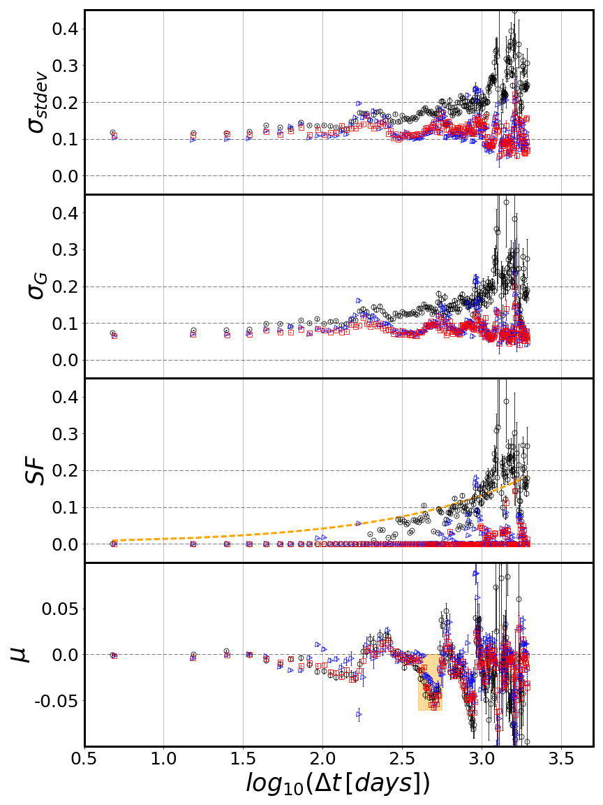
The top two panels in Fig. 2 show the standard deviation for $\Delta m$, and the robust standard deviation ($\sigma_{G}=0.741(q_{75}-q_{25})$, where $q_{25}$ and $q_{75}$ are 25% and 75% quartiles) estimate computed from the interquartile range, as a function of $\Delta t$ for quasars, and separately for blue and red stars. $\sigma_{G}$ is somewhat smaller than the standard deviation, which indicates mild non-Gaussianity of $\Delta m$ distributions. For $\Delta t$ below about 100 d, all three subsamples show similar behaviour, while for longer time-scales quasars show appreciably larger scatter of observed $\Delta m$ due to intrinsic variability. In order to estimate the intrinsic variability, these “raw” measurements need to be corrected for the effects of observational (measurement) errors, as described next.

3.1 Effects of observational errors on SF

Given a bin with $M$ values of ($\Delta t_{i}$, $\Delta m_{i}$, $e_{i}$), $i=1...M$, SF will correspond to the rms width of the $\Delta m_{i}$ distribution, $\sigma_{tot}$, only if all $e_{i}$ are negligibly small compared to the true SF value. When measurement uncertainties are homoscedastic, $e_{i}=\bar{e}$, then simply SF = $(\sigma_{tot}^{2}-\bar{e}^{2})^{1/2}$. In a general case of heteroscedastic uncertainties, the correction for the effects of observational errors is more involved because each value $\Delta m_{i}$ is drawn from a different Gaussian distribution whose width is given by $\sigma_{i}=(\rm{SF}^{2}+e_{i}^{2})^{1/2}$. Indeed, in this general case the distribution of all $\Delta m_{i}$ in a given bin need not be a Gaussian at all!

We refer the reader for a detailed discussion of how to estimate SF in a general case to Ivezić et al. (2014), and here briefly summarize the gist of their maximum likelihood method. The likelihood of a set of $M$ measurements $\Delta m_{i}$ is given by

$$p(\{\Delta m_{i}\}|\rm{SF},\mu,\{e_{i}\})=\prod_{i=1}^{M}{\frac{1}{\sqrt{2\pi}\sigma_{i}}\exp{\left(\frac{-(\Delta m_{i}-\mu)^{2}}{2\sigma_{i}^{2}}\right)}},$$ (5)

where $\{.\}$ denotes a set of values and $\mu$ is introduced to account for possible systematic photometric errors between observing epochs that define the bin’s $\Delta t_{i}$ values. We note that this expression is only an approximation to the true likelihood because it assumes that measurement errors for $\Delta m_{i}$ are uncorrelated. This assumption is, strictly speaking, not true because different $\Delta m_{i}$ values can be based on the same individual magnitude measurements. In practice, the covariance between errors can introduce a bias in maximum likelihood solutions, but only for $M$ much larger than used here these errors become not negligible compared to the SF. Indeed, we used the same maximum likelihood method as Schmidt et al. (2010), equation(2), that assumes no correlation between errors.

There is no closed form solution for maximizing the likelihood given by equation 5 and we estimate SF numerically, using code from astroML python module (Vanderplas et al., 2012). With the aid of Bayes Theorem and using uniform priors for SF and $\mu$, the logarithm of the posterior probability distribution function (pdf) for SF and $\mu$ becomes

$$L_{p}(SF,\mu)={\rm const.}-{1\over 2}\sum_{i=1}^{M}\left(\ln(\rm{SF}^{2}+e_{i}^{2})+{(\Delta m_{i}-\mu)^{2}\over\rm{SF}^{2}+e_{i}^{2}}\right).$$ (6)

We evaluate $L_{p}$ on a grid of $\mu$ and SF first, find its maximum that yields the maximum a posteriori (MAP) estimates for SF and $\mu$, and then marginalize over $\mu$ to find the posterior pdf for SF as

$$p(\rm{SF})=\int_{0}^{\infty}{p(\rm{SF},\mu|\{\Delta m_{i}\},\{e_{i}\})}d\mu,$$ (7)

which is used to estimate the uncertainty (the credible region) of MAP estimate for SF. When there is no strong evidence for intrinsic variability, SF tends to zero.

Figure 2: The four panels show various statistics computed for subsamples of 747 CRTS quasars (black circles), 1496 ‘blue’ stars (blue triangles), and 2327 ‘red’ stars (red squares), with SDSS $r$ magnitudes in the range 18.5-19. Red and blue stars have SDSS colours $1<\mathrm{g-i}<3$ and $-1<\mathrm{g-i}<1$, respectively. All pairwise CRTS brightness differences are binned in 200 linearly spaced bins of time difference $\Delta t$. For each bin, we compute, from top to bottom: the standard deviation $\sigma_{stdev}$, the robust standard deviation estimate $\sigma_{G}$ based on the interquartile range , the structure function SF, and the mean value of $\Delta m$ per bin $\mu$. The statistical (random) errors are often smaller than the symbol size due to large number of data points; systematic errors for all displayed quantities are probably of the order 0.01 mag (not shown). Both $\mu$ and SF are found from the two-dimensional maximum of the log-likelihood $L_{p}$ on the $[\mu,\rm{SF}]$ grid (see equation 6). The yellow dashed line in the third panel traces the fiducial DRW model (see equation 1). We address the peculiar wiggle behaviour in the Appendix B, but it does not have any influence on our overall conclusions.

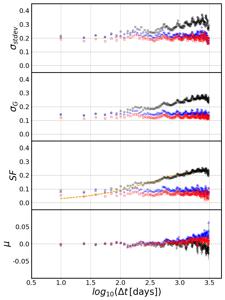
The bottom two panels in Fig. 2 show SF and $\mu$ as a function of $\Delta t$ for quasars, blue and red stars. For $\Delta t$ below about 1000 d, $\mu$ for all three subsamples is within 0.01 mag from zero, as expected. On the other hand, SF below about 100 d is in the range 0.05-0.10 mag for all three subsamples. In the case of quasars, the observed SF$\sim$0.1 mag for 10 d $<\Delta t<$100 d demonstrates that the difference between SDSS results from MacLeod et al. (2010) (see the yellow dashed line in the third panel) and CRTS results from Graham et al. (2014) is not due to different analysis methods (SF versus SWV, respectively): Here, we fully reproduce this discrepancy using the SF method and CRTS data.

Fig. 2 also indicates a plausible solution to this puzzle: the observed SF for both blue and red stars in the range 10${}^{d}<\Delta t<$100^d is unexpectedly large: The values are in the range 0.05–0.10 mag rather than negligible (say, $\la 0.01-0.02$ mag). In other words, more variation is observed in light curves of non-variable stars than can be explained with reported photometric errors. The same result is obtained for all three chosen magnitude bins. Such a behaviour could be observed if photometric error estimates computed by the CRTS photometric pipeline are mis-estimated, resulting in an incorrect correction for observational errors. We proceed to perform an independent test of photometric errors using repeated observations of non-variable standard stars.

3.2 Tests of observational errors using non-variable stars

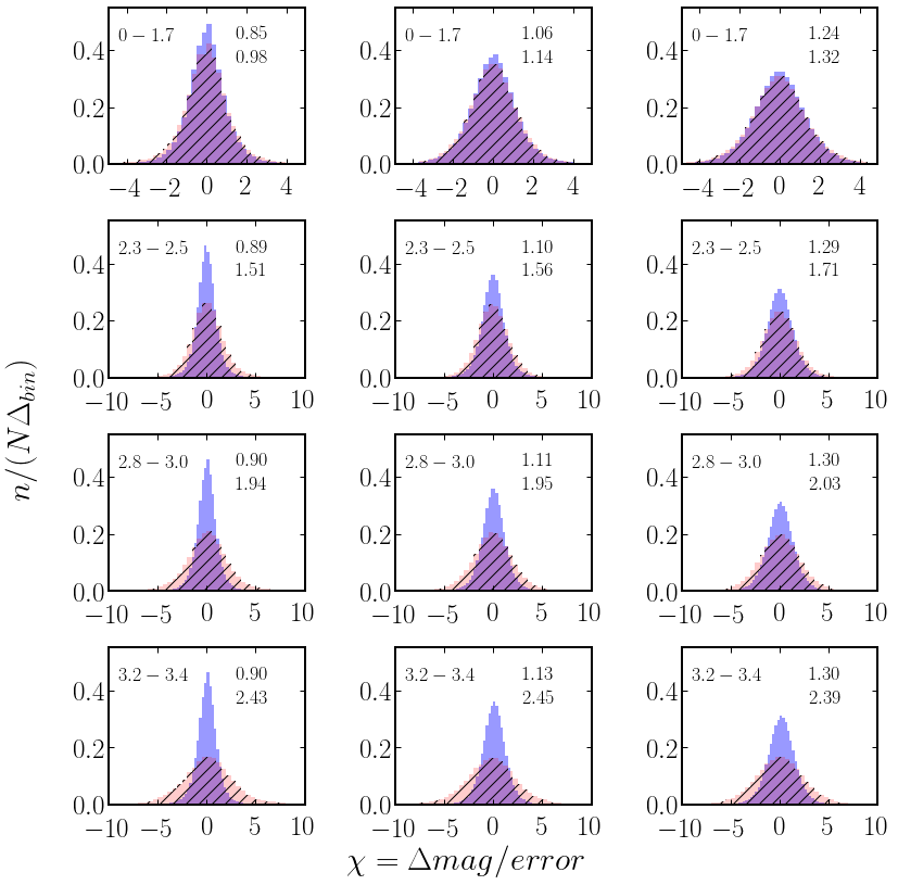
Assuming that standard stars from SDSS are truly non-variable, if (Gaussian) photometric error estimates computed by the CRTS photometric pipeline are correct, then the distribution of $\chi_{i}=\Delta m_{i}/e_{i}$ for stars should be distributed as a unit Gaussian, $N$(0,1). Deviations of the distribution width for stars from unity indicate incorrect photometric error estimates. For quasars, we expect that the width should exceed unity because of their intrinsic variability, and that the width should increase with $\Delta t$. We perform this test in Fig. 3, where we show $\chi$ distributions for both blue stars and quasars, and for a grid of $\Delta t$ and magnitude bins.

For the shortest $\Delta t$ bin ($<$50 d), the distributions for stars and quasars appear indistinguishable for all three magnitude bins. This similarity immediately argues that there is no detected intrinsic variability for quasars. Furthermore, the width of $\chi$ distributions for stars appears to be a function of magnitude, with very little dependence on $\Delta t$. The distribution widths for stars in each magnitude bin (all $\Delta t$ values), obtained using robust width estimator $\sigma_{G}$, are listed in Table 2. For example, the bin with $18.5<r<19$, which contains the majority of quasars, appears to have under-estimated photometric errors by a factor of 1.3, on average. The same conclusion is derived using red stars. For small $\Delta t$, where quasar SF is intrinsically small, the quasar SF will be thus significantly over-estimated, while for large $\Delta t$, where the quasar SF is intrinsically large, the effect on SF will be small. We extend this qualitative conclusion to a more quantitative analysis in the next section.

We note that problems with CRTS photometric uncertainty estimates have been reported before (e.g., Vaughan et al. 2016). Additional analysis of CRTS photometric uncertainty estimates, beyond magnitude limits of direct interest to quasar variability analysis, is presented in Appendix A.

Table 2: The robust distribution widths for $\chi$ for blue stars.

Magnitude	$\sigma_{G}$
17–18	0.870
18–18.5	1.107
18.5–19	1.288

Figure 3: Histograms show CRTS-based $\chi=\Delta m/\mathrm{error}$ for blue stars (blue shading) and quasars (red hatched shading), split into bins of $\log{\Delta t}$ (rows) and SDSS $r$ magnitude (columns). Vertically, from top to bottom, $\log{\Delta t}$ : $0<\log{\Delta t}<1.7$ ($t<50$ days), $2.3<\log{\Delta t}<2.5$, $2.8<\log{\Delta t}<3.0$, and $3.2<\log{\Delta t}<3.4$ (indicated by numbers in the upper left-hand corner of each subplot). Horizontally, from the left- to right-hand side, the SDSS $r$ magnitude bins are: $17-18$, $18-18.5$, and $18.5-19$. The numbers in the upper right-hand corner of each subplot are the robust width of $\chi$ distributions determined using interquartile range ($\sigma_{G}$); upper value for blue stars and lower value for quasars.

3.3 SF with corrected observational errors

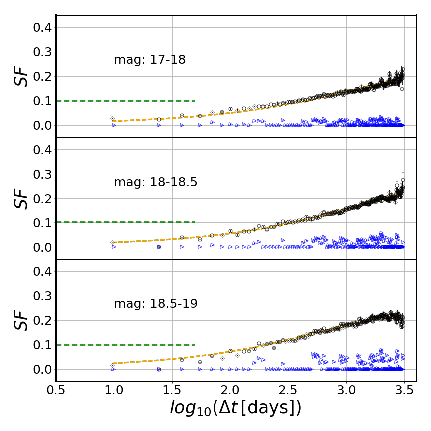
Informed by the analysis from preceding section, we assume that correction factors for photometric error estimates are independent of colour and are only a function of magnitude. Depending on the magnitude of stars and quasars, we multiply their reported photometric errors by $\sigma_{G}$ values listed in Table 2, and repeat SF analysis. By construction, we expect that the width of $\chi$ distributions for blue stars will be unity, and that their SF will tend to 0. For quasars, compared to SF values shown in the third panel in Fig. 2, we expect somewhat smaller SF at large $\Delta t$ and much smaller SF at small $\Delta t$.

Fig. 4 shows SF for blue stars and quasars for subsamples from the three selected magnitude bins. As evident, both expectations are born out: for all three magnitude bins, SF for blue stars is essentially vanishing within noise ($\sim$0.05 mag), while SF for quasars at small $\Delta t$ is about twice smaller than in Fig. 2 and thus consistent with the values based on SDSS data. In Fig. 5, we demonstrate that this agreement with SDSS results extends to rest frame analysis, too.

Figure 4: Analogous to the third panel in Fig. 2, except that here SF for blue stars and quasars in all three magnitude bins are shown, and photometric errors are modified by multiplicative correction factors listed in Table 2. Note that SF for stars in vanishing, while SF for quasars at $\log_{10}(\Delta t)<1.7$ is about twice as small as in Fig. 2.

Figure 5: Analogous to Fig. 4, but here for $\Delta t$ in the quasar rest frame : t_rest = t_obs / (1+$z$), using known quasar redshifts from SDSS (MacLeod et al., 2010). The rest frame correction shifts time lags to shorter time-scales and produces SF for quasars in agreement with corresponding results obtained by MacLeod et al. 2010.

3.4 SF estimated from PTF data

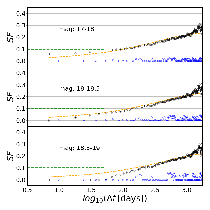
Recent PTF (Palomar Transient Factory) Data Release 3 light curves can be used for an independent test of our conclusions derived above. We queried the NASA/IPAC Infrared Science Archive ‘PTF Objects’ catalogue using coordinates for 7601 spectroscopically confirmed Stripe 82 quasars, and 48 250 standard stars (same as the final samples used for CRTS-based analysis). A positional multi-object search with a matching radius of 2 arcsec, with a flag ‘ngoodobs’ $>$ 10, resulted in 6471 quasars and 38 776 stars. For these objects, we obtained time series data from the ‘PTF Light Curve Table’ catalogue (we grouped by SDSS coordinates).

We processed these PTF light curves in exactly the same way as the CRTS light curves. We first performed day-averaging, using the weighted error as the measure of uncertainty on day-averaged brightness measurement. We further selected only those objects that have been observed on at least 10 different nights, resulting in samples of 2753 quasars and 15 714 stars. The counts of magnitude-limited subsamples are listed in Table 3.

Table 3: Count of stars and quasars, selected by their SDSS $r$ magnitudes and $g$–$i$ colours. Analoguous to Table 1, except that here the counts of stars and quasars with PTF adequate data are listed.

$r$ magnitude	Red stars	Blue stars	Quasars
17–18	1243	1077	90
18–18.5	825	497	160
18.5–19	913	548	377
Total	2981	2122	627

The SF results based on PTF light curve data are shown in Fig. 6. For these uncorrected PTF data, it is evident that there is no sign of variability for quasars on short time-scales ($\Delta t<100\,d$) above the SDSS-level of $\sim$0.05 mag (unlike for CRTS data, see Fig. 2). Note also that standard stars show no appreciable variability at any time-scale (SF$\approx 0$). Therefore, this PTF-based analysis further supports our conclusion that extraneous quasar variability at short time-scales was due to slightly underestimated photometric uncertainties.

Figure 6: Analogous to Fig. 2, but here the statistics for subsamples of 377 quasars (black circles), 548 ‘blue’ stars (blue triangles), and 913 ‘red’ stars (red squares), with adequate PTF light curve data are shown. Note that the mean magnitude difference ($\mu$, the bottom panel) does not stay as close to 0 as for CRTS data – a deviation around $\log_{10}\Delta t\approx 2.7$ might indicate some issues with photometric zero-point calibration (at the level of 0.02–0.03 mag).

4 Conclusions

We analysed the error properties of the CRTS sample of quasars and standard stars. Using repeated CRTS observations of non-variable stars, we found that the photometric error estimates computed by the CRTS photometric pipeline are slightly under-estimated for the majority of quasars. When quasar light curves are corrected for the impact of observational errors, the resulting corrections to the SF are thus too small. For small $\Delta t$, where quasar SF is intrinsically small, quasar SF is significantly over-estimated (akin to the subtraction of two large numbers to get a small number, when the second large number is under-estimated). In particular, at time-scales of about 50 d, SF is over-estimated by about a factor of 2. This behaviour provides a plausible explanation for the increased quasar variability level in CRTS light curves reported by Graham et al. (2014), compared to earlier SDSS-based results obtained by MacLeod et al. (2010). An additional analysis based on independent light curve data for the same objects obtained by the PTF provides further support for this conclusion. We conclude that the quasar variability constraints on weekly and monthly time-scales from SDSS, CRTS and PTF surveys are mutually compatible, as well as consistent with DRW model.

Appendix A Variation of the CRTS photometric uncertainty with magnitude

We found in Section 3.2 (see Table 2) that reported CRTS photometric uncertainty estimates are too large by $\sim$15% in the magnitude range 17–18, and too small by $\sim$10-25% in the magnitude range 18–19. Such problems have been reported before; for example, Vaughan et al. (2016) reported that for bright objects (magnitude $\sim$15) the error bars provided by the CRTS pipeline processing are overestimated by a factor of 4-5. Since this factor is much larger than we obtained for fainter magnitude bins, we extend our standard star analysis to the full CRTS magnitude range.

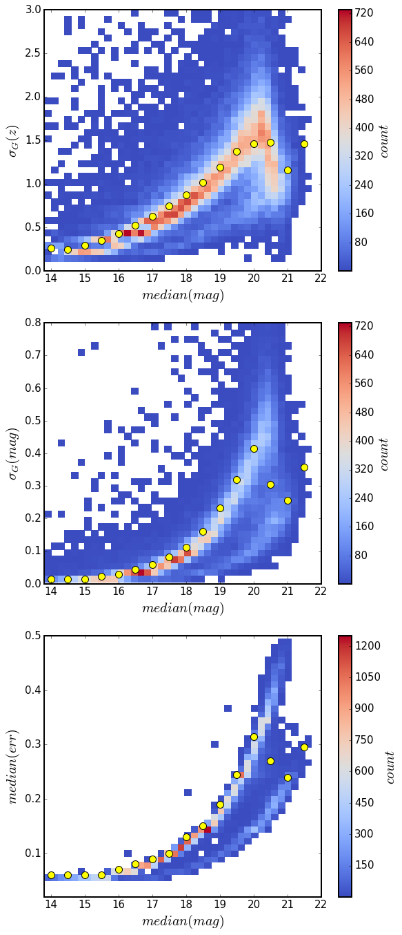
The top panel in Fig. 7 shows the variation with magnitude of the robust distribution width for the quantity

$$z_{ij}={m_{ij}-m_{j}\over err_{ij}},$$ (8)

where $m_{j}$ is the weighted mean magnitude for star indexed $j$, and index $i$ runs over all observations of a given star. The quantity $\sigma_{G}(z)_{j}$ is the robust quartile-based distribution width of $z_{ij}$ for a given star $j$. If the reported CRTS photometric uncertainties ($err_{ij}$) were correctly estimated, the $\sigma_{G}(z)$ distribution for standard (non-variable) stars would be centred on unity and independent of magnitude. As the top panel in Fig. 7 clearly demonstrates this is not the case: $\sigma_{G}(z)$ is $\sim$0.25 at the bright end, and increases to $\sim$1.5 at the faint end. In the magnitude range 17–19, the $\sigma_{G}(z)$ behaviour is consistent with the results listed in Table 2.

The middle and bottom panels show that the observed intrinsic scatter per light curve at the bright end is $\sim 0.01$ mag, while reported photometric uncertainty is never smaller than 0.05 mag. In other words, we confirm the result reported by Vaughan et al. (2016) for the bright end and demonstrate that problems with reported CRTS photometric uncertainties are a strong function of magnitude.

Figure 7: The top panel shows the variation with magnitude of the photometric scatter per light curve, normalized by reported CRTS photometric uncertainties (see equation 8 for definition), using CRTS light curves for $\sim$48,000 standard (non-variable) stars from the SDSS catalogue. If the reported CRTS photometric uncertainties were correctly estimated, the $\sigma_{G}(z)$ distribution would be centred on unity and independent of magnitude. The middle panel shows the observed intrinsic scatter per light curve, and the bottom panel shows the distribution of reported photometric uncertainty, both as function of median magnitude (per light curve).

Appendix B CSS calibration wiggles

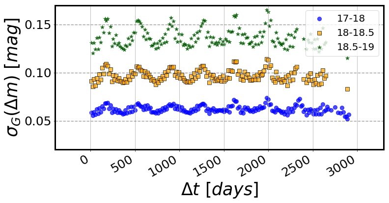
We saw an oscillatory pattern on plots of SF and standard deviation using CRTS data on Figs. 2, 4 and 5. We ruled out any astrophysical origin since the effect also persisted when using only standard stars. Despite an anti-correlation of the pattern with the number of points per bin, we ruled out the statistical origin by fixing the number of points per bin. Fig. 8 shows that wiggles persists even if we set the number of points per $\Delta t$ bin to 20 000. We see the effect when points are separated by (2k+1)/2 yr, with $k$=0,1,2 … . We conclude that this variation is related to the airmass which fluctuates seasonally, which was not properly accounted for in the CSS calibration process. This is because the primary aim of CSS was to detect moving objects, which requires only intranight consistency, and not long-term accuracy (Drake et al., 2013).

Figure 8: Robust standard deviation for CRTS standard stars, showing that the oscillatory pattern persists even with fixed number of points per bin. We combine the ‘blue’ and ‘red’ subsamples (-1$<g-i<$3), yielding 5788, 3487 and 3823 stars in SDSS $r$-magnitude bins bright (green stars) medium (orange squares) and faint (blue circles), respectively (see Table 1 for counts in individual subsamples). For each $\Delta t$ bin, we randomly select 20 000 $\Delta m$ points. If there are less than 20 000 points in a bin, we do not plot anything (this affects less than 35 bins per magnitude bin, mostly towards longer time-scales). It illustrates that the wiggles are purely due to seasonal differences, and possibly hidden zero-point errors, unaccounted for in the CSS pipeline. This pattern does not change our overall conclusions.

References

- Abazajian et al. (2009) Abazajian K. N., et al., 2009, ApJS, 182, 543
- Charisi et al. (2016) Charisi M., Bartos I., Haiman Z., Price-Whelan A. M., Graham M. J., Bellm E. C., Laher R. R., Márka S., 2016, MNRAS, 463, 2145
- Collier & Peterson (2001) Collier S., Peterson B. M., 2001, ApJ, 555, 775
- Djorgovski et al. (2011) Djorgovski S. G., et al., 2011, preprint (arXiv:1102.5004),
- Drake et al. (2013) Drake A. J., et al., 2013, ApJ, 763, 32
- Graham et al. (2013) Graham M. J., Drake A. J., Djorgovski S. G., Mahabal A. A., Donalek C., Duan V., Maker A., 2013, MNRAS, 434, 3423
- Graham et al. (2014) Graham M. J., Djorgovski S. G., Drake A. J., Mahabal A. A., Chang M., Stern D., Donalek C., Glikman E., 2014, MNRAS, 439, 703
- Graham et al. (2015) Graham M. J., et al., 2015, MNRAS, 453, 1562
- Hawkins (2002) Hawkins M. R. S., 2002, MNRAS, 329, 76
- Hawkins (2007) Hawkins M. R. S., 2007, A&A, 462, 581
- Ivezić et al. (2004) Ivezić Ž., et al., 2004, in Storchi-Bergmann T., Ho L. C., Schmitt H. R., eds, IAU Symposium Vol. 222, The Interplay Among Black Holes, Stars and ISM in Galactic Nuclei. pp 525–526 (arXiv:astro-ph/0404487), doi:10.1017/S1743921304003126
- Ivezić et al. (2007) Ivezić Ž., et al., 2007, AJ, 134, 973
- Ivezić et al. (2014) Ivezić Ž., Connolly A. J., VanderPlas J. T., Gray A., 2014, Statistics, Data Mining, and Machine Learning in Astronomy, Princeton Univ. Press, Princeton and Oxford
- Kawaguchi et al. (1998) Kawaguchi T., Mineshige S., Umemura M., Turner E. L., 1998, ApJ, 504, 671
- Kelly et al. (2007) Kelly B. C., Bechtold J., Siemiginowska A., Aldcroft T., Sobolewska M., 2007, ApJ, 657, 116
- Kelly et al. (2009) Kelly B. C., Bechtold J., Siemiginowska A., 2009, The Astrophysical Journal, 698, 895
- Kelly et al. (2011) Kelly B. C., Sobolewska M., Siemiginowska A., 2011, ApJ, 730, 52
- Kozłowski (2016) Kozłowski S., 2016, ApJ, 826, 118
- Lawrence (2016) Lawrence A., 2016, in Mickaelian A., Lawrence A., Magakian T., eds, Astronomical Society of the Pacific Conference Series Vol. 505, Astronomical Surveys and Big Data. p. 107 (arXiv:1605.09331)
- MacLeod et al. (2010) MacLeod C. L., et al., 2010, The Astrophysical Journal, 721, 1014
- MacLeod et al. (2011) MacLeod C. L., et al., 2011, The Astrophysical Journal, 728, 26
- MacLeod et al. (2012) MacLeod C. L., et al., 2012, The Astrophysical Journal, 753, 106
- Rau et al. (2009) Rau A., et al., 2009, PASP, 121, 1334
- Schmidt et al. (2010) Schmidt K. B., Marshall P. J., Rix H.-W., Jester S., Hennawi J. F., Dobler G., 2010, ApJ, 714, 1194
- Schneider et al. (2010) Schneider D. P., et al., 2010, VizieR Online Data Catalog, 7260
- Vanden Berk et al. (2004) Vanden Berk D. E., et al., 2004, ApJ, 601, 692
- Vanderplas et al. (2012) Vanderplas J., Connolly A., Ivezić Ž., Gray A., 2012, in Conference on Intelligent Data Understanding (CIDU). pp 47 –54, doi:10.1109/CIDU.2012.6382200
- Vaughan et al. (2016) Vaughan S., Uttley P., Markowitz A. G., Huppenkothen D., Middleton M. J., Alston W. N., Scargle J. D., Farr W. M., 2016, MNRAS, 461, 3145
- Zu et al. (2013) Zu Y., Kochanek C. S., Kozłowski S., Udalski A., 2013, ApJ, 765, 106
- de Vries et al. (2005) de Vries W. H., Becker R. H., White R. L., Loomis C., 2005, AJ, 129, 615