A Bayesian statistical analysis of stochastic phenotypic plasticity model of cancer cells

Da Zhou¹, Shanjun Mao², Jing Cheng³, Kaiyi Chen¹, Xiaofang Cao¹, Jie Hu^1,∗

1. School of Mathematical Sciences, Xiamen University, Xiamen 361005, P.R. China
   ($*$Corresponding Author, hujiechelsea@xmu.edu.cn))

2. Department of Statistics, The Chinese University of Hong Kong, Shatin, N.T., Hong Kong, PR China

3. School of Statistics, Huaqiao University, Xiamen 361005, P.R. China

Abstract

The phenotypic plasticity of cancer cells has received special attention in recent years. Even though related models have been widely studied in terms of mathematical properties, a thorough statistical analysis on parameter estimation and model selection is still very lacking. In this study, we present a Bayesian approach on the relative frequencies of cancer stem cells (CSCs). Both Gibbs sampling and Metropolis-Hastings (MH) algorithm are used to perform point and interval estimations of cell-state transition rates between CSCs and non-CSCs. Extensive simulations demonstrate the validity of our model and algorithm. By applying this method to a published data on SW620 colon cancer cell line, the model selection favors the phenotypic plasticity model, relative to conventional hierarchical model of cancer cells. Moreover, it is found that the initial state of CSCs after cell sorting significantly influences the occurrence of phenotypic plasticity.

1 Introduction

The hypothesis of cancer stem cell theory [1, 2] postulates a hierarchical organization of cancer cells. A small number of tumorigenic cancer cells, also termed cancer stem cells (CSCs), reside at the apex of this cellular hierarchy [3]. CSCs are capable of self-renewal and generating more differentiated cancer cells with lower tumorigenic potential. However, growing researches have extended the CSC model by proposing a phenotypic plasticity paradigm in which reversible transitions could happen between CSCs and non-CSCs [4]. That is, not only can CSCs give rise to non-CSCs, but a fraction of non-CSCs can reacquire CSC-like characteristics. This de-differentiation from non-CSCs to CSCs has been reported in quite a few types of cancer, such as breast cancer [5, 6, 7], melanoma [8], colon cancer [9], and glioblastoma multiforme [10].

Very recently special attention has been paid to reasonable mathematical models for quantifying the process of phenotypic plasticity. In particular, it was found that the phenotypic plasticity plays an important role in the stability of the quantitative models [6, 11, 12, 13, 14, 15, 16]. That is, the phenotypic plasticity greatly contributes to stabilizing the phenotypic mixture of cancer cells, thereby effectively maintaining the heterogeneity of cancer cell populations. Some other researches laid emphasis on the role of the phenotypic plasticity in transient dynamics. It was shown that an interesting overshoot phenomenon of CSCs observed in experiment can be well explained by de-differentiation from non-CSCs to CSCs [17, 18]. Besides, Leder et al studied mathematical models of pdgf-driven glioblastoma and revealed that the effectiveness of radiotherapy is quite sensitive to the capability of de-differentiation from differentiated sensitive cells to stem-like resistant cells [19]; Jilkine and Gutenkunst studied the effect of de-differentiation on time to mutation acquisition in cancers [20]; Chen et al studied transition model between endocrine therapy responsive and resistant states in breast cancer by Landscape Theory [21]; Dhawan et al showed with mathematical modeling that exposure to hypoxia enhanced the plasticity and heterogeneity of cancer cell populations [22]; Tonekaboi et al investigated how cellular plasticity behaves differently in small and large cancer cell populations [23]. A recent review by Jolly et al [24] focused on quantitative models of Epithelial-mesenchymal plasticity in cancer.

Even though the phenotypic plasticity has been extensively studied in terms of mathematical properties, the statistical analysis on parameter estimation and model selection is still very lacking. Actually, one of the crucial tasks in the research of phenotypic plasticity is to estimate the transition rates between different cell types. As a pioneering work, Gupta et al [6] established a discrete-time Markov state transition model and estimated the transition probabilities between different cell states by fitting the model to their FACS (Fluorescence-activated cell sorting) data on SUM159 and SUM149 breast cancer cell lines. Besides, continuous-time ordinary differential equations (ODEs) models were also developed [13, 14], based on which de-differentiation rates were estimated by fitting to SW620 colon cancer cell line. However, the above mentioned works can only provide point estimations to the interested parameters, but not interval estimations. Comparatively, interval estimation is much more informative and frequently-used than point estimation in practice. For doing interval estimation, statistical modeling rather than deterministic modeling should be applied. Moreover, note that it is still questionable if de-differentiation is a crucial improvement to the cellular hierarchy of cancer cells or just a minor extension to it, model selection can be used to validate the paradigm of phenotypic plasticity in terms of statistical significance. Therefore, a thorough statistical analysis is of great value for further quantifying the biological process of phenotypic plasticity and exploring its biological significance.

In this research, a statistical framework is presented to analyze a two-phenotypic model of cancer cells. In this model, each cancer cell is either CSC phenotypic state or non-CSC phenotypic state. Both types of cells can divide symmetrically or asymmetrically with certain probabilities. A Bayesian approach [25] is developed to fit this model to experimental data on relative frequencies of CSCs. MCMC methods (such as Gibbs sampling [26] and MH algorithm [27, 28]) are used to perform statistical inference with Multivariate Potential Scale Reduction Factor (MPSRF) [29, 30] checking the convergence of MCMC chains. Our simulation results demonstrate the precision and accuracy of our algorithm by both point estimation and interval estimation. By applying our approach to a published data on SW620 colon cancer cell line [9], we also perform model selection via deviance information criterion (DIC, [31]). Our result shows that the phenotypic plasticity model with de-differentiation has superior quality relative to the hierarchical model without de-differentiation. Furthermore, an interesting frequency-dependent phenomenon is presented, i.e. the estimated values of the model parameters depend on the initial relative frequencies of different cell states. This suggests that the process of phenotypic plasticity could be relevant to the heterogeneity level of cancer cell populations.

The paper is organized as follows. The model assumptions and Bayesian framework are presented in Section 2. Main results including simulations and real data analysis are shown in Section 3. Conclusions are presented in Section 4.

2 Methods

2.1 Model assumptions

In this section we describe the model assumptions. Note that the salient feature of the phenotypic plasticity model is the reversibility between CSCs and non-CSCs, i.e., not only can CSCs differentiate into non-CSCs, but non-CSCs are also capable of de-differentiating into CSCs. Consider a population of cancer cells comprising two phenotypes: CSC represents cancer stem cell phenotypic state, non-CSC represents non-stem cancer cell phenotypic state. Even though this two-phenotypic assumption simplifies the biological complexity of highly diverse phenotypes in cancer, the two-phenotypic setting has been proved as an effective and reasonable simplification for highlighting the minimal process of phenotypic plasticity [11, 12, 13, 19]. Similar bidirectional transition cascade models were also studied in bacterial community [32, 33].

We now present the cellular process of the two-phenotypic model. From probabilistic point of view, this model can be seen as a discrete-time two-type branching process [34]. Each cell lives for a fixed time (suppose one unit of time). At the moment of death it gives birth to two daughter cells. More specifically, for each CSC, it gives birth to two identical CSC daughter cells with probability $\alpha$ (symmetric division), otherwise (with probability $1-\alpha$) it gives birth to one CSC daughter cell and one non-CSC daughter cell (asymmetric division). For each non-CSC, it divides symmetrically into two non-CSC daughter cells with probability $1-\beta$, whereas it divides asymmetrically into one non-CSC daughter cell and one CSC daughter cell with probability $\beta$ (de-differentiation). The model will reduce to conventional hierarchical model if letting $\beta=0$, i.e. de-differentiation is not allowed to happen. Hence the model selection with respect to $\beta$ provides an efficient way to evaluate the significance of phenotypic plasticity.

The statistical inference of branching processes has been studied for a long time [35]. The usage of statistical methods strongly depends on the data types available. Normally, the observation of the whole genealogy tree generated from underlying process is quite difficult to obtain (except in very limited experiments [36]). Instead, only can the numbers or relative frequencies of distinct cell types be recorded at given moment, and comparatively it is easier to collect data on relative frequencies than absolute numbers of given cell types [37]. Thus developing statistical approaches for proportion data has a wider range of application. In this work our proposed method is used for the time-series data on relative frequencies of CSC phenotypic state.

Let $x_{A}(t)$ be the frequency of CSC state at time $t$, $\mu_{t}$ be the expectation of $x_{A}(t)$, i.e. $\mu_{t}=\textbf{E}(x_{A}(t))$, and $\sigma^{2}_{t}$ be the variance of $x_{A}(t)$, i.e. $\sigma^{2}_{t}=\textbf{Var}(x_{A}(t))$. Then we can obtain two important recurrence formulas as follows (see A for more details):

$$\mu_{t+1}=\frac{1+\alpha-\beta}{2}\mu_{t}+\frac{\beta}{2},$$ (1)

$$\sigma^{2}_{t+1}=(\frac{1+\alpha-\beta}{2})^{2}\sigma^{2}_{t}+\frac{1}{N_{0}\times 2^{t+2}}\left\{[\alpha(1-\alpha)-\beta(1-\beta)]\mu_{t}+\beta(1-\beta)\right\},$$ (2)

where $N_{0}$ is the initial number of the whole population. In next section, we will put forward a Bayesian statistical framework based on the above two formulas.

2.2 Bayesian framework

The data we deal with looks like $\{(m_{0},v_{0}),(m_{1},v_{1}),\cdots,(m_{t},v_{t}),\cdots(m_{T},v_{T})\}$, where $m_{t}$ and $v_{t}$ are sample mean and sample variance of $n$ realizations of $x_{A}(t)$ respectively. The Markov property of the model implies that the distribution of data at time $t$ only depends on data at time $t-1$. Thus, we can write the joint likelihood of data as follows:

$$L(\alpha,\beta|m_{0},v_{0},m_{1},v_{1},\cdots,m_{T},v_{T})=f(m_{0},v_{0})\times f(m_{1},v_{1}|m_{0},v_{0},\alpha,\beta)\times\cdots\times f(m_{T},v_{T}|m_{T-1},v_{T-1},\alpha,\beta).$$

Note that $f(m_{0},v_{0})$ is irrelevant to the parameters $\alpha$ and $\beta$, the joint likelihood can be expressed as

$$L(\alpha,\beta|m_{0},v_{0},m_{1},v_{1},\cdots,m_{T},v_{T})\propto f(m_{1},v_{1}|m_{0},v_{0},\alpha,\beta)\times\cdots\times f(m_{T},v_{T}|m_{T-1},v_{T-1},\alpha,\beta).$$

According to the asymptotic normality of $x_{A}(t)$ provided $N_{0}\gg 1$ (see Theorem 1 in [37]), the asymptotic distributions of $m_{t}$ and $v_{t}$ can be given as:

$$m_{t}\sim N(\mu_{t},\frac{\sigma^{2}_{t}}{n}),$$

$$v_{t}\sim\frac{\sigma^{2}_{t}}{n-1}\chi^{2}(n-1).$$

Since $m_{t},v_{t}$ are unbiased estimators of $\mu_{t},\sigma^{2}_{t}$ respectively, we can substitute $\mu_{t}$ and $\sigma^{2}_{t}$ with the corresponding observed sample mean $m_{t}$ and sample variance $v_{t}$ in the recurrence formulas (1) and (2). Given the priors of $\alpha,\beta$ as $Beta(1,1)$, i.e. uniform distribution, we can obtain the following posterior distribution:

$$p(\alpha,\beta|m_{0},v_{0},m_{1},v_{1}\cdots,m_{T},v_{T})=L(\alpha,\beta|m_{0},v_{0},m_{1},v_{1},\cdots,m_{T},v_{T})\times p(\alpha)\times p(\beta)$$

$$\propto \prod_{t=0}^{T-1}\left\{\left[\left(\frac{1+\alpha-\beta}{2}\right)^{2}v_{t}+\frac{1}{N_{0}\times 2^{t+2}}\left\{[\alpha(1-\alpha)-\beta(1-\beta)]m_{t}+\beta(1-\beta)\right\}\right]^{-\frac{n}{2}}v_{t+1}^{\frac{n-3}{2}}\right\}\times$$

$$\exp\left\{-\frac{1}{2}\sum_{t=0}^{T-1}\frac{n(m_{t+1}-\frac{1+\alpha-\beta}{2}m_{t}-\frac{\beta}{2})^{2}}{(\frac{1+\alpha-\beta}{2})^{2}v_{t}+\frac{1}{N_{0}\times 2^{t+2}}\left\{[\alpha(1-\alpha)-\beta(1-\beta)]m_{t}+\beta(1-\beta)\right\}}+\right.$$

$$\left.\frac{(n-1)v_{t+1}}{(\frac{1+\alpha-\beta}{2})^{2}v_{t}+\frac{1}{N_{0}\times 2^{t+2}}\left\{[\alpha(1-\alpha)-\beta(1-\beta)]m_{t}+\beta(1-\beta)\right\}}\right\}$$

Note that $N_{0}\gg 1$, the above posterior distribution can be revised as the following simplified expression:

$$p(\alpha,\beta|m_{0},v_{0},m_{1},v_{1}\cdots,m_{T},v_{T}) \propto \prod_{t=0}^{T-1}\left\{\left[\left(\frac{1+\alpha-\beta}{2}\right)^{2}v_{t}\right]^{-\frac{n}{2}}v_{t+1}^{\frac{n-3}{2}}\right\}\times$$

$$\exp\left\{-\frac{1}{2}\sum_{t=0}^{T-1}\frac{n(m_{t+1}-\frac{1+\alpha-\beta}{2}m_{t}-\frac{\beta}{2})^{2}}{(\frac{1+\alpha-\beta}{2})^{2}v_{t}}+\frac{(n-1)v_{t+1}}{(\frac{1+\alpha-\beta}{2})^{2}v_{t}}\right\}$$

We will show in Section 3.2 that $N_{0}$ does has little impact on the simulation results, and then validate the above simplified posterior distribution.

Based on the proposed posterior distribution, $\alpha$ and $\beta$ are sampled iteratively by Gibbs sampling and MH algorithm. We draw several sample chains independently and apply MPSRF [29, 30] to check the convergence of MCMC chains. If the MCMC chains converge, we obtain the point estimation and interval estimation as mean value and interval between $2.5\%$ and $97.5\%$ quantiles of converged posterior samples respectively.

3 Results

In this section we perform some simulations to validate our algorithm and also apply our method to a published data set of SW620 colon cancer cell line [9].

3.1 Simulation I

In the first simulation, we generate synthesized data sets to test the performance of our algorithm. In particular, we set $N_{0}=10^{4}$ and generate parameters $\alpha$ and $\beta$ from their priors respectively, drawing mean value $m_{0}$ from $Unif(0.3,0.7)$ and standard deviance $v_{0}^{\frac{1}{2}}$ from $Unif(0.01,0.03)$. We then synthesize $\{m_{1},v_{1}\},\cdots,\{m_{T},v_{T}\}$ sequentially based on the conditional distribution function in Section 2.2. In all we generate 100 groups of parameters and each group consists of 20 simulations. Table 1 demonstrates the estimation results including Mean Square Error (MSE) of point estimation, averaged length of $95\%$ confidence intervals (AL) and mean proportion of interval estimation covering the true value of parameters (CR).

$\alpha$			$\beta$
MSE	AL	CR	MSE	AL	CR
0.0004	0.0414	0.924	0.0003	0.0321	0.917

Table 1: Estimation results of Simulation I.

It is easy to find that our algorithm is accurate for the synthesized data sets, with small MSE, high coverage rate and narrow confidence interval.

3.2 Simulation II

In the second simulation, we generate data sets by following the cellular processes of the two-phenotypic model described in Section 2.1 to validate our method. We set $N_{0}=10^{4}$ and randomly generate the true values of parameters $\alpha$ and $\beta$ from their priors. Given each value of $(\alpha,\beta)$ and initial state $x_{A}(0)$ sampled from a Normal distribution $N(\mu^{\prime},\sigma^{\prime 2})$ with $\mu^{\prime}\sim Unif(0.3,0.7)$ and $\sigma^{\prime}\sim Unif(0.01,0.03)$, we generate $n=5$ synthesized realizations of $x_{A}(t)$ and then calculate the sample mean $m_{t}$ and sample variance $v_{t}$ as algorithm input. In all we generate 100 groups of parameters $(\alpha,\beta)$ with each consisting of 20 simulations. Table 2 demonstrates the MSE, AL and CR of two methods with and without $N_{0}$ as known true value.

Set	$\alpha$			$\beta$
	MSE	AL	CR	MSE	AL	CR
With $N_{0}$	0.0004	0.0380	0.979	0.0002	0.0302	0.979
Without $N_{0}$	0.0006	0.0378	0.962	0.0003	0.0296	0.963

Table 2: Estimation results of Simulation II.

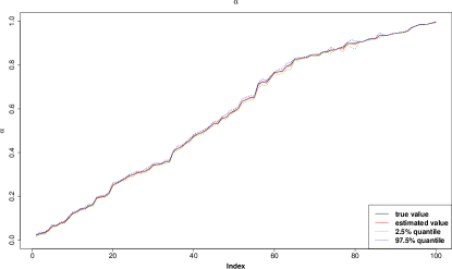
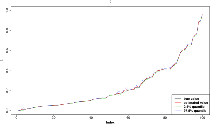
From the table, we can see that our algorithm well captures the cellular process when only mean and variance data are available. Both point estimation and interval estimation achieve high accuracy even if $N_{0}$ is unknown in our algorithm. An example of estimation results can be found in B.

3.3 Real data

Our real data application is based on a published data of SW620 colon cancer cell line (see Figure 4A in [9]). There are four groups of data in this experiment. In each group, CSC proportions were measured via FACS (Fluorescence-activated cell sorting), and both sample mean $m_{t}$ and sample variance $v_{t}$ were recorded successively. The four groups differ in the initial states of relative frequencies: (A) $0.6\%$ CSCs and $99.4\%$ non-CSCs; (B) 70% CSCs and 30% non-CSCs; (C) $99.4\%$ CSCs and $0.6\%$ non-CSCs; (D) $65.4\%$ CSCs and $34.6\%$ non-CSCs. We assume four sets of parameters $\Theta_{1}=\{\alpha_{1},\beta_{1}\},\Theta_{2}=\{\alpha_{2},\beta_{2}\},\Theta_{3}=\{\alpha_{3},\beta_{3}\},\Theta_{4}=\{\alpha_{4},\beta_{4}\}$ corresponding to four groups of data and perform model selection by calculating Deviance information criterion (DIC, [31]). As a generalization of Akaike information criterion (AIC) and Bayesian information criterion (BIC), DIC is also an estimator of the relative quality of statistical models for given data, and it is particularly useful in Bayesian statistical settings, representing the trade-off between the error of fitting and the complexity of the model. The smaller the DIC is, the more favorable the model is.

Our primary concern is whether the hypothesis of reversible phenotypic plasticity is superior to the hypothesis of cellular hierarchy given the colon cancer data. Note that the phenotypic plasticity model will reduce to the hierarchical model by setting $\beta_{i}=0$ ($i=1,2,3,4$). We would like to compare the DIC values between the full model and the hierarchical model without de-differentiation. Our result shows that the DIC value of the full model is $-103.23$, which is smaller than that of the hierarchical model without de-differentiation ($-84.05$). Model selection thus suggests that de-differentiation significantly improve the quality of the model for the given data.

Furthermore, we are interested in whether some of the four groups of data share the common values of the parameters, from which we can see the dependency of the parameters on the initial states. The DIC values of different models are shown in Table 3 (see C for the estimated values of the parameters). From the table, we can find that models $\Theta_{1}\neq\Theta_{2}\neq\Theta_{3}\neq\Theta_{4}$ and $\Theta_{1}=\Theta_{2}$ obtain the smallest DIC values, which means these two models are favorable. Due to the limited data length, these two models cannot be distinguished since the difference between their DIC values is only about 0.15, without statistical significance. It is interesting that the model $\Theta_{1}\neq\Theta_{2}\neq\Theta_{3}\neq\Theta_{4}$ is selected as the favorable model. That is, none of the four groups share the common parameters, all the parameters are sensitive to the initial states of relative frequencies. Note that different initial relative frequencies correspond to different states of phenotypic heterogeneity at the beginning of cell sorting, our result suggests an interesting heterogeneity-dependency of the phenotypic plasticity model.

Model	DIC
$\Theta_{1}\neq\Theta_{2}\neq\Theta_{3}\neq\Theta_{4}$	-103.23
$\Theta_{1}=\Theta_{2}$	-103.38
$\Theta_{1}=\Theta_{3}$	7.03
$\Theta_{1}=\Theta_{4}$	-90.00
$\Theta_{2}=\Theta_{3}$	125.37
$\Theta_{2}=\Theta_{4}$	-82.37
$\Theta_{3}=\Theta_{4}$	71.72
$\Theta_{1}=\Theta_{2},\Theta_{3}=\Theta_{4}$	71.57
$\Theta_{1}=\Theta_{3},\Theta_{2}=\Theta_{4}$	27.89
$\Theta_{1}=\Theta_{4},\Theta_{2}=\Theta_{3}$	138.60
$\Theta_{2}=\Theta_{3}=\Theta_{4}$	173.39
$\Theta_{1}=\Theta_{3}=\Theta_{4}$	96.39
$\Theta_{1}=\Theta_{2}=\Theta_{4}$	-83.58
$\Theta_{1}=\Theta_{2}=\Theta_{3}$	146.96
$\Theta_{1}=\Theta_{2}=\Theta_{3}=\Theta_{4}$	189.42

Table 3: DIC of Bayesian model selection.

4 Conclusions

We have presented a Bayesian statistical analysis on a stochastic phenotypic plasticity model of cancer cells. Both simulation studies and real data analysis have shown the power of our method. Compared to the deterministic models in previous studies [14, 13], the stochastic model here equipping with statistical inference makes quantitative modeling in a more sophisticated way. On one hand, parameter estimation is extended from point-level into interval-level. On the other hand, model selection provides a systematic means to compare different models, and then helps to evaluate different biological hypotheses.

It should be noted that, the two-phenotypic model is a very simplified model. By focusing on our attention to the reversibility between CSCs and non-CSCs, many biologically complex mechanisms are not included in this model. For example, the model is discrete-time, ignoring the complicated time distribution of cell cycle [38, 39, 40]. Developing feasible Bayesian framework for more complicated models could be of great value in future researches.

Appendix A Derivation of Eqs. (1) and (2)

Here we present the mathematical details of how to obtain Eqs. (1) and (2), i.e. the recurrence formulas of the expectation and variance of $x_{A}(t)$.

Let $n_{A}(t)$ and $n_{B}(t)$ are the numbers of CSC and non-CSC states, $x_{A}(t)$ and $x_{B}(t)$ are the frequencies of CSC and non-CSC states, $N(t)$ is the population size of the whole population. It is easy to know that $x_{A}(t)=1-x_{B}(t)$, $x_{A}(t)=n_{A}(t)/N(t)=n_{A}(t)/(n_{A}(t)+n_{B}(t))$, and $x_{B}(t)=n_{B}(t)/N(t)$. Suppose

$$\xi_{i}=\left\{\begin{array}[]{ll}1,&\hbox{with probability $\alpha$}\\ 0,&\hbox{with probability $1-\alpha$}\end{array}\right.$$

$$\eta_{i}=\left\{\begin{array}[]{ll}1,&\hbox{with probability $\beta$}\\ 0,&\hbox{with probability $1-\beta$,}\end{array}\right.$$

then we have

$$n_{A}(t+1)=n_{A}(t)+\sum_{i=1}^{n_{A}(t)}\xi_{i}+\sum_{i=1}^{n_{B}(t)}\eta_{i}.$$

By taking conditional expectation on both sides we have

$$E(n_{A}(t+1)|n_{A}(t))=n_{A}(t)+n_{A}(t)\times\alpha+n_{B}(t)\times\beta.$$

Then for the conditional expectation of $x_{A}(t)$ we have

$$E(x_{A}(t+1)|x_{A}(t)) = E(\frac{n_{A}(t+1)}{N(t+1)}|x_{A}(t))$$

$$= E(\frac{n_{A}(t+1)}{2N(t)}|x_{A}(t))$$

$$= \frac{1}{2}\frac{1}{N(t)}(n_{A}(t)+n_{A}(t)\times\alpha+n_{B}(t)\times\beta)$$

$$= \frac{1}{2}(x_{A}(t)+x_{A}(t)\times\alpha+x_{B}(t)\times\beta)$$

$$= \frac{1}{2}(1+\alpha)x_{A}(t)+\frac{1}{2}(1-x_{A}(t))\beta$$

$$= \frac{1+\alpha-\beta}{2}x_{A}(t)+\frac{\beta}{2}.$$

With the law of total expectation we obtain Eq. (1) as follows

$$\mu_{t+1}=E(x_{A}(t))=E(E(x_{A}(t+1)|x_{A}(t)))=\frac{1+\alpha-\beta}{2}\mu_{t}+\frac{\beta}{2}.$$

For the conditional variance of $x_{A}(t)$,

$$Var(x_{A}(t+1)|x_{A}(t)) = Var(\frac{n_{A}(t+1)}{N(t+1)}|x_{A}(t))$$

$$= Var(\frac{n_{A}(t)+\sum_{i=1}^{n_{A}(t)}\xi_{i}+\sum_{i=1}^{n_{B}(t)}\eta_{i}}{N(t+1)}|x_{A}(t))$$

$$= Var(\frac{\sum_{i=1}^{n_{A}(t)}\xi_{i}+\sum_{i=1}^{n_{B}(t)}\eta_{i}}{N_{0}\times 2^{t+1}}|x_{A}(t))$$

$$= \frac{1}{N_{0}^{2}\times 2^{2t+2}}(n_{A}(t)\alpha(1-\alpha)+n_{B}(t)\beta(1-\beta))$$

$$= \frac{1}{N_{0}\times 2^{t+2}}(\frac{n_{A}(t)}{N_{0}\times 2^{t}}\alpha(1-\alpha)+\frac{n_{B}(t)}{N_{0}\times 2^{t}}\beta(1-\beta))$$

$$= \frac{1}{N_{0}\times 2^{t+2}}(x_{A}(t)\alpha(1-\alpha)+x_{B}(t)\beta(1-\beta))$$

With the law of total variance we obtain Eq. (2) as follows

$$\sigma^{2}_{t+1} = Var(E(x_{A}(t+1)|x_{A}(t)))+E(Var(x_{A}(t+1)|x_{A}(t)))$$

$$= (\frac{1+\alpha-\beta}{2})^{2}\sigma^{2}_{t}+\frac{1}{N_{0}\times 2^{t+2}}\left\{[\alpha(1-\alpha)-\beta(1-\beta)]\mu_{t}+\beta(1-\beta)\right\}.$$

Appendix B An example of simulation results

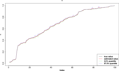
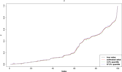
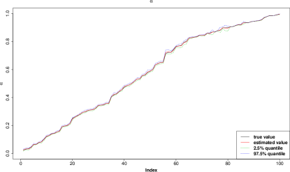
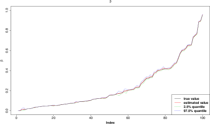
We select one simulation from each of the 20 parameters settings in Simulations I$\&$II, and show an example of estimation results in Figure 1.

(a) Simulation I: $\alpha$

(b) Simulation I: $\beta$

(c) Simulation II with $N_{0}$: $\alpha$

(d) Simulation II with $N_{0}$: $\beta$

(e) Simulation II without $N_{0}$: $\alpha$

(f) Simulation II without $N_{0}$: $\beta$

Figure 1: An example of estimation results in Simulation I and Simulation II. Black solid lines represent true values of parameters and red lines represent point estimation. And two dashed lines demonstrate interval estimations. For Simulation II, both the estimation results with and without $N_{0}$ are shown

Appendix C Point estimation of real data

Here we show point estimation results of real data for different models.

Model	$\alpha$	$\beta$
$\Theta_{1}$	0.978	0.125
$\Theta_{2}$	0.990	0.118
$\Theta_{3}$	0.890	0.008
$\Theta_{4}$	0.991	0.014
$\Theta_{1}=\Theta_{2}$	0.987	0.121
$\Theta_{1}=\Theta_{3}$	0.889	0.056
$\Theta_{1}=\Theta_{4}$	0.992	0.031
$\Theta_{2}=\Theta_{3}$	0.899	0.072
$\Theta_{2}=\Theta_{4}$	0.993	0.036
$\Theta_{3}=\Theta_{4}$	0.902	0.064
$\Theta_{1}=\Theta_{2}=\Theta_{3}$	0.882	0.154
$\Theta_{1}=\Theta_{2}=\Theta_{4}$	0.996	0.042
$\Theta_{1}=\Theta_{3}=\Theta_{4}$	0.888	0.131
$\Theta_{2}=\Theta_{3}=\Theta_{4}$	0.900	0.116
$\Theta_{1}=\Theta_{2}=\Theta_{3}=\Theta_{4}$	0.892	0.152

Table 4: Parameter estimation of different models. $\Theta_{i}$ represents the estimation of parameters of $i$-th group in real data and $\Theta_{i_{1}}=\cdots=\Theta_{i_{k}}$ represents estimation of common parameters within these $k$ groups.

References

- [1] T. Reya, S. Morrison, M. Clarke, I. Weissman, Stem cells, cancer, and cancer stem cells, Nature 414 (2001) 105–111.
- [2] C. Jordan, M. Guzman, M. Noble, Cancer stem cells, N. Engl. J. Med. 355 (12) (2006) 1253–1261.
- [3] P. Dalerba, R. Cho, M. Clarke, Cancer stem cells: models and concepts, Annu. Rev. Med. 58 (2007) 267–284.
- [4] N. D. Marjanovic, R. A. Weinberg, C. L. Chaffer, Cell plasticity and heterogeneity in cancer, Clin. Chem. 59 (1) (2013) 168–179.
- [5] M. Meyer, J. Fleming, M. Ali, M. Pesesky, E. Ginsburg, B. Vonderhaar, Dynamic regulation of cd24 and the invasive, cd44poscd24neg phenotype in breast cancer cell lines, Breast Cancer Res. 11 (6) (2009) R82.
- [6] P. Gupta, C. Fillmore, G. Jiang, S. Shapira, K. Tao, C. Kuperwasser, E. Lander, Stochastic state transitions give rise to phenotypic equilibrium in populations of cancer cells, Cell 146 (4) (2011) 633–644.
- [7] C. L. Chaffer, N. D. Marjanovic, T. Lee, G. Bell, C. G. Kleer, F. Reinhardt, A. C. D Alessio, R. A. Young, R. A. Weinberg, Poised chromatin at the zeb1 promoter enables breast cancer cell plasticity and enhances tumorigenicity, Cell 154 (1) (2013) 61–74.
- [8] E. Quintana, M. Shackleton, H. R. Foster, D. R. Fullen, M. S. Sabel, T. M. Johnson, S. J. Morrison, Phenotypic heterogeneity among tumorigenic melanoma cells from patients that is reversible and not hierarchically organized, Cancer cell 18 (5) (2010) 510–523.
- [9] G. Yang, Y. Quan, W. Wang, Q. Fu, J. Wu, T. Mei, J. Li, Y. Tang, C. Luo, Q. Ouyang, et al., Dynamic equilibrium between cancer stem cells and non-stem cancer cells in human sw620 and mcf-7 cancer cell populations, Br. J. Cancer 106 (9) (2012) 1512–1519.
- [10] E. Fessler, T. Borovski, J. P. Medema, Endothelial cells induce cancer stem cell features in differentiated glioblastoma cells via bfgf, Mol. cancer 14 (1) (2015) 157.
- [11] R. V. dos Santos, L. M. da Silva, A possible explanation for the variable frequencies of cancer stem cells in tumors, PloS One 8 (8) (2013) e69131.
- [12] R. V. dos Santos, L. M. da Silva, The noise and the kiss in the cancer stem cells niche, J. Theor. Biol. 335 (21) (2013) 79–87.
- [13] W. Wang, Y. Quan, Q. Fu, Y. Liu, Y. Liang, J. Wu, G. Yang, C. Luo, Q. Ouyang, Y. Wang, Dynamics between cancer cell subpopulations reveals a model coordinating with both hierarchical and stochastic concepts, PLoS One 9 (1) (2014) e84654.
- [14] D. Zhou, Y. Wang, B. Wu, A multi-phenotypic cancer model with cell plasticity, J. Theor. Biol. 357 (2014) 35–45.
- [15] J. X. Zhou, A. O. Pisco, H. Qian, S. Huang, Nonequilibrium population dynamics of phenotype conversion of cancer cells, PLoS One 9 (12) (2014) e110714.
- [16] Y. Niu, Y. Wang, D. Zhou, The phenotypic equilibrium of cancer cells: From average-level stability to path-wise convergence, J. Theor. Biol. 386 (2015) 7–17.
- [17] A. L. Sellerio, E. Ciusani, N. B. Benmoshe, S. Coco, A. Piccinini, C. R. Myers, J. P. Sethna, C. Giampietro, S. Zapperi, C. A. M. L. Porta, Overshoot during phenotypic switching of cancer cell populations, Sci. Rep. 5 (2015) 15464.
- [18] X. Chen, Y. Wang, T. Feng, M. Yi, X. Zhang, D. Zhou, The overshoot and phenotypic equilibrium in characterizing cancer dynamics of reversible phenotypic plasticity, J. Theor. Biol. 390 (2016) 40–49.
- [19] K. Leder, K. Pitter, Q. LaPlant, D. Hambardzumyan, B. D. Ross, T. A. Chan, E. C. Holland, F. Michor, Mathematical modeling of pdgf-driven glioblastoma reveals optimized radiation dosing schedules, Cell 156 (3) (2014) 603–616.
- [20] A. Jilkine, R. N. Gutenkunst, E. Wang, Effect of dedifferentiation on time to mutation acquisition in stem cell-driven cancers, PLoS Comput. Biol. 10 (3) (2014) e1003481.
- [21] C. Chen, W. T. Baumann, J. Xing, L. Xu, R. Clarke, J. J. Tyson, Mathematical models of the transitions between endocrine therapy responsive and resistant states in breast cancer, J. R. Soc. Interface. 11 (96) (2014) 20140206.
- [22] A. Dhawan, S. A. M. Tonekaboni, J. H. Taube, S. Hu, N. Sphyris, S. A. Mani, M. Kohandel, Mathematical modelling of phenotypic plasticity and conversion to a stem-cell state under hypoxia, Sci. Rep. 6 (2016) 18074.
- [23] S. A. M. Tonekaboni, A. Dhawan, M. Kohandel, Mathematical modelling of plasticity and phenotype switching in cancer cell populations, Math. Biosci. 283 (2017) 30–37.
- [24] M. Jolly, S. Tripathi, J. Somarelli, S. Hanash, H. Levine, Epithelial-mesenchymal plasticity: How have quantitative mathematical models helped improve our understanding?, Mol. Oncol. 11 (7) (2017) 739–754.
- [25] P. D. Hoff, A First Course in Bayesian Statistical Methods, Springer, New York, 2009.
- [26] S. Geman, D. Geman, Stochastic relaxation, gibbs distributions, and the bayesian restoration of images, IEEE T. Pattern. Anal. PAMI-6 (6) (1987) 564–584.
- [27] N. Metropolis, A. W. Rosenbluth, M. N. Rosenbluth, A. H. Teller, E. Teller, Equation of state calculations by fast computing machines, J Chem. Phys. 21 (6) (1953) 1087–1092.
- [28] W. K. Hastings, Monte carlo sampling methods using markov chains and their applications, Biometrika 57 (1) (1970) 97–109.
- [29] A. Gelman, D. B. Rubin, Inference from iterative simulation using multiple sequences, Stat. Sci. 7 (4) (1992) 457–472.
- [30] S. P. Brooks, A. Gelman, General methods for monitoring convergence of iterative simulations, J Comput. Graph. Stat. 7 (4) (1998) 434–455.
- [31] A. Gelman, J. B. Carlin, H. S. Stern, e. Rubin, Donald B., Bayesian Data Analysis, Second Edition (Texts in Statistical Science), Chapman and Hall/CRC, Boca Raton, 2003.
- [32] Q. M. Pei, X. Zhan, L. J. Yang, J. Shen, L. F. Wang, K. Qui, T. Liu, J. B. Kirunda, A. A. Yousif, A. B. Li, Fluctuation and noise propagation in phenotypic transition cascades of clonal populations., Phys. Rev. E 92 (1) (2015) 012721.
- [33] J. Mao, A. E. Blanchard, T. Lu, Slow and steady wins the race: a bacterial exploitative competition strategy in fluctuating environments, ACS Synth. Biol. 4 (3) (2015) 240.
- [34] P. Haccou, P. Jagers, V. A. Vatutin, Branching processes: variation, growth, and extinction of populations, Cambridge University Press, Cambridge, 2005.
- [35] P. Guttorp, Statistical inference for branching processes, Wiley, New York, 1991.
- [36] J. Hu, Z. Zhao, H. K. Yalamanchili, J. Wang, K. Ye, X. Fan, Bayesian detection of embryonic gene expression onset in c. elegans, Ann. Appl. Stat. 9 (2) (2015) 950.
- [37] A. Y. Yakovlev, N. M. Yanev, Relative frequencies in multitype branching processes, Ann. App. Prob. 19 (1) (2009) 1-14.
- [38] C. J. Mode, Multitype branching processes : theory and applications, Elsevier, New York, 1971.
- [39] A. Golubev, Exponentially modified gaussian (emg) relevance to distributions related to cell proliferation and differentiation., J. Theor. Biol. 262 (2) (2010) 257–266.
- [40] D. Q. Jiang, Y. Wang, D. Zhou, Phenotypic equilibrium as probabilistic convergence in multi-phenotype cell population dynamics., Plos One 12 (2) (2017) e0170916.