Composite Quantization
Abstract
This paper studies the compact coding approach to approximate nearest neighbor search. We introduce a composite quantization framework. It uses the composition of several () elements, each of which is selected from a different dictionary, to accurately approximate a -dimensional vector, thus yielding accurate search, and represents the data vector by a short code composed of the indices of the selected elements in the corresponding dictionaries. Our key contribution lies in introducing a near-orthogonality constraint, which makes the search efficiency is guaranteed as the cost of the distance computation is reduced to from through a distance table lookup scheme. The resulting approach is called near-orthogonal composite quantization. We theoretically justify the equivalence between near-orthogonal composite quantization and minimizing an upper bound of a function formed by jointly considering the quantization error and the search cost according to a generalized triangle inequality. We empirically show the efficacy of the proposed approach over several benchmark datasets. In addition, we demonstrate the superior performances in other three applications: combination with inverted multi-index, quantizing the query for mobile search, and inner-product similarity search.
Index Terms:
Approximate Nearest Neighbor Search, Quantization, Composite Quantization, Near-Orthogonality.1 Introduction
Nearest neighbor (NN) search has been a fundamental research topic in machine learning, computer vision, and information retrieval [31]. The goal of NN search, given a query , is to find a vector whose distance to the query is the smallest from -dimensional reference (database) vectors.
The straightforward solution, linear scan, is to compute the distances to all the database vectors whose time cost is and is very time-consuming, and thus impractical for large scale high-dimensional cases. Multi-dimensional indexing methods, such as the -d tree [6], have been developed to speed up exact search. For high-dimensional cases it turns out that such approaches are not much more efficient (or even less efficient) than linear scan.
Approximate nearest neighbor (ANN) search has been attracting a lot of interests because of competitive search accuracy and tractable storage and search time cost. The algorithms can be split into two main categories: (1) accelerating the search by comparing the query with a small part of reference vectors through an index structure, such as random -d trees [32], FLANN [25], and neighborhood graph [34]; and (2) accelerating the distance computation between the query and the reference vectors through the compact coding technique, i.e., converting the database vectors into short codes, with typical solutions including hashing [10, 40, 23, 33], quantization [16, 27, 42].
In this paper, we introduce a composite quantization framework to convert vectors to compact codes. The idea is to approximate a vector using the composition (addition) of elements each selected from one dictionary, and to represent this vector by a short code composed of the indices of the selected elements. The way of adding the selected dictionary elements is different from concatenating the selected dictionary elements (subvectors) adopted in product quantization [16] and its extensions, Cartesian -means [27] and optimized product quantization [7], that divide the space into partitions and conduct -means separately over each partition to obtain the dictionaries. The advantage is that the vector approximation, and accordingly the distance approximation of a query to the database vector, is more accurate, yielding more accurate nearest neighbor search.
To efficiently evaluate the distance between a query and the short code representing the database vector, we first present a naive solution, called orthogonal composite quantization, by introducing orthogonality constraints, i.e., the dictionaries are mutually orthogonal. The benefit is that the approximated distance can be calculated from the distance of the query to each selected element, taking only a few distance table lookups, and that the time cost is reduced to from . Furthermore, we propose a better solution, called near-orthogonal composite quantization, by relaxing orthogonality constraints to near-orthogonality constraints, i.e., the summation of the inner products of all pairs of elements that are used to approximate the vector but from different dictionaries is constant. The distance computation is still efficient, while the distance approximation is more accurate, and accordingly the search accuracy is higher.
The resulting near-orthogonal composite quantization (NOCQ) is justified in both theory and experiments. We present a generalized triangle inequality, theoretically explaining that near-orthogonal composite quantization is equivalent to minimizing an upper bound of a function that is formed by jointly considering the quantization error and the search time cost. We also show that production quantization [16] and Cartesian -means [27] are constrained versions of NOCQ: NOCQ relaxes the orthogonality constraint between dictionaries and does not require the explicit choice of the dimension of each subspace corresponding to each dictionary. We present empirical results over several standard datasets demonstrate that the proposed approach achieves state-of-the-art performances in approximate nearest neighbor search in terms of the Euclidean distance. In addition, we demonstrate the superior performances in other three applications: combination with inverted multi-index, quantizing the query for mobile search, and inner-product similarity search.
2 Related work
A comprehensive survey on learning to hash is given in [37], showing that the quantization algorithms [16, 27, 35, 37] achieve better search quality than hashing algorithms with Hamming distance, even with optimized or asymmetric distances [12, 36]. Thus, this paper only presents a brief review of the quantization algorithms.
Hypercubic quantization, such as iterative quantization [10], isotropic hashing [20], harmonious hashing [39], angular quantization [8], can be regarded as a variant of scalar quantization by optimally rotating the data space and performing binary quantization along each dimension in the rotated space, with the quantization centers fixed at and (or equivalently and ). Such a way of fixing quantization centers puts a limit on the number of possible distances in the coding space, which also limits the accuracy of distance approximation even using optimized distances [12, 36]. Therefore, the overall search performance is not comparable to product quantization and Cartesian -means.
Product quantization [16] divides the data space into (e.g., ) disjoint subspaces. Accordingly, each database vector is divided into subvectors, and the whole database is also split into sub-databases. A number of clusters are obtained by conducting -means over each sub-database. Then a database vector is approximated by concatenating the nearest cluster center of each subspace, yielding a representation with a short code containing the indices of the nearest cluster centers. The computation of the distance between two vectors is accelerated by looking up a precomputed table.
Cartesian -means [27] (or optimized product quantization [7]) improves the compositionabilty, i.e., vector approximation accuracy, by finding an optimal feature space rotation and then performing product quantization over the rotated space. Additive quantization [1, 5] further improves the compositionabilty by approximating a database vector using the summation of dictionary elements selected from different dictionaries, whose idea is similar to structured vector quantization [13] (a.k.a., multi-stage vector quantization and residual quantization). It has been applied to data compression [1] and inner product similarity search [5], yet is not suitable for search with Euclidean distance due to the lack of the acceleration of distance computation.
There are other attempts to improve product quantization in the other ways, such as distance-encoded product quantization [14] and locally optimized product quantization [19], which can also be combined with our approach in the same way. The hash table scheme is studied in [24] to accelerate the linear scan over the product quantization codes. Inverted multi-index [3] applies product quantization to build an inverted index for searching a very large scale database, with the ability of efficiently retrieving the candidates from a large number of inverted lists. Bilayer product quantization [4] improves the efficiency of distance computation within the inverted multi-index framework. We will also apply the proposed approach to inverted multi-index to show its effectiveness.
This paper represents a very substantial extension of our previous conference paper [42]111The terminology in this paper is different from the conference paper. with the introduction of alternative versions of near-orthogonal composite quantization, and an additional material added from our report [5]. The main technical novelties compared with [42] lie in three-fold. (1) We introduce two alternative objective functions: one is from the strict orthogonality constraint, and the other is from the generalized triangle inequality. (2) We present extensive analysis of composite quantization, including why quantization is proper for approximate nearest neighbor search, why multiple different dictionaries rather than a single dictionary are used. (3) We conduct more experiments, such as quantizing the query for mobile search, and inner-product similarity search.
3 Preliminaries
Approximate nearest neighbor search. Nearest neighbor (NN) search is a problem of, given a query vector , finding a vector from a set of -dimensional reference vectors , such that its distance to the query vector is minimum, i.e., . Here, is a distance between and , and the Euclidean distance is a typical example. Approximate nearest neighbor (ANN) search, the focus of this paper, aims efficiently find a good guess of the exact nearest neighbor rather than the exact one.
Compact coding. The search cost of the naive linear scan algorithm is , where comes from the distance evaluation . Compact coding in general is a low-dimensional embedding approach and represents an input vector by a short descriptor . Here is the parameters, and could be a binary representation vector or a sequence of () binary codes, e.g., where is a byte-valued variable. The application of compact coding to approximate nearest neighbor search uses the distance computed in the code space, as an substitute of the distance in the input space, to rank the reference vectors. The benefit is that the distance computation cost in the compact code space is reduced to , where , and consequently the search efficiency is improved.
Quantization. Quantization is a process of mapping a large set of input vectors to a countable (smaller) set of representative vectors (e.g., ), called dictionary. For instance, a reference vector is mapped to a dictionary element, , such that the reconstruction error is minimal, , and accordingly can be represented by a short code . Quantization has been widely adopted in image and signal compression.
As a compact coding approach, quantization is successfully applied to approximate nearest neighbor search by using the asymmetric distance between the query and the quantized vector , , to approximate the original distance, . The search accuracy is guaranteed by the following theorem.
Theorem 1 (Triangle inequality).
The reconstruction error of the distances is upper-bounded: .
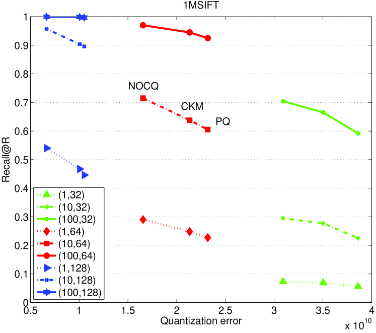
This suggests that the quantization error is an upper bound of the distance reconstruction error, and thus the search accuracy depends on the quantization quality: low quantization error usually leads to high search accuracy. An empirical comparison in terms of the quantization error (i.e., ) vs. the search accuracy among product quantization (PQ), cartesian k-means (CKM), and our approach, near-orthogonal composite quantization (NOCQ), is shown in Figure 1. We can see that the proposed approach is able to achieve lower quantization error and hence has better search performance.
Cartesian quantization. The state-of-the-art approach, which we call Cartesian quantization, constructs the dictionary from several (e.g., ) small dictionaries , called source dictionary, where (for simplicity, we assume ), through the Cartesian product operation, , where -tuples form the composite dictionary. The benefits include that several small dictionaries generate a larger composite dictionary, with the consequence that the quantization error can be smaller and that the encoding time is reduced while a longer code (larger dictionary) is actually used.
In contrast to the application to compression whose goal is to reconstruct the vector from the compact code, the application to approximate nearest neighbor search aims to accelerate the distance reconstruction. Typically, the distance between a query and a -tuple that approximates a vector , is computed from the distances through looking up the distance table recording the distances between the query and the elements in the source dictionary, which reduces the time cost from to .
Our proposed approach belongs to this Cartesian quantization category, which also contains the product quantization [16] and Cartesian -means [27] (or optimized product quantization [7]), in which the dictionaries are mutual-orthogonal. The novelty of our approach lies in adopting the addition scheme to form the composite dictionary element from the -tuples, which removes the mutual orthogonality constraint between the dictionaries, and introducing the near-orthogonality condition to theoretically guarantee the efficiency of the distance reconstruction.
4 Formulation
Composite quantization. Our approach forms the composite dictionary element from the -tuples through an addition operation, . A vector is approximated as
| (1) |
where is the index of the element selected from the source dictionary for the th reference vector . We find the dictionary by minimizing
| (2) |
Given the approximation through composite quantization, , the distance of a query to the approximation is
| (3) |
It is time-consuming to reconstruct the approximate vector (taking ) and then compute the distance between and (taking ). In the following, we introduce two solutions to accelerate the distance computation.
Orthogonal composite quantization. We introduce an extra constraint, mutual orthogonality of the subspaces, each spanned by the corresponding dictionary:
| (4) |
where is the matrix form of the th dictionary. We show that composite quantization with this constraint, called orthogonal composite quantization (OCQ), makes the distance computation efficient.
Let be the subspace spanned by the dictionary . Assume that the subspaces cover the whole -dimensional space. The query is then transformed as below,
| (5) |
The distance between the query and the approximate database vector is calculated in the following way,
| (6) |
Consequently, the cost of the distance computation is reduced from to by looking up the precomputed table storing the distances between the query and the dictionary elements in each subspace.
Near-orthogonal composite quantization. We expand the distance computation into three terms:
| (7) | |||
| (8) |
We can see that, given the query , the second term in the right-hand side, , is constant for all the database vectors. and hence is unnecessary to compute for nearest neighbor search.
The first term is the summation of the distances of the query to the selected dictionary elements, and can be efficiently computed using a few () additions by looking up a distance table, where the distance table, , is precomputed before comparing the query with each reference vector, and stores the distances of the query to the dictionary elements,
Similarly, we can build a table storing the inner products between dictionary elements,
and compute the third term using distance table lookups. This results in the distance computation cost is changed from to , which is still large. For instance, in the case where and , is larger than , which means that the cost is greater than that using the original vector.
It can be seen that with the orthogonality constraint (4) the third term is equal to :
| (9) |
Thus, the computation cost is reduced to . We notice that, if the third term is a constant,
| (10) |
called near-orthogonality, the third term can be discarded for the distance computation. Consequently, we only need to compute the first term for nearest neighbor search, and the computation cost is also reduced to . The resulting approach is called near-orthogonal composite quantization (NOCQ). The goal is to minimize the quantization errors (problem (2)) subject to the near-orthogonality constraint (10).
Near-orthogonality can be viewed as a relaxation of strict orthogonality because Equation (10) (near-orthogonality) is a necessary but not sufficient condition of Equation (4) (strict orthogonality) while Equation (4) is a sufficient but not necessary condition of Equation (10). Thus, the vector approximation with the relaxed condition, near-orthogonality, is more accurate. Empirical comparisons in Table II show that the vector approximation and accordingly the distance approximation of NOCQ is more accurate than OCQ.
Joint accuracy and efficiency optimization. We first introduce several notations. (1) The square root of the first term in the right-hand side of Equation (8) is denoted by :
(2) The square root of the summation of the square of the true Euclidean distance and a query-dependent term is written as
(3) Accordingly we define the approximate version,
(4) The third term in the right-hand side of Equation (8) is denoted as : .
The near-orthogonal composite quantization approach uses as the distance for nearest neighbor search, which is essentially an approximation of (with dropped) as we have, by definition,
and thus an approximation of . Notice that only depends on the true distance between and and a query-dependent term that is a constant for the search with a specific query. Ideally, if , the search accuracy would be .
In general, the absolute difference is expected to be small to guarantee high search accuracy. We have the following theorem:
Theorem 2 (Generalized triangle inequality).
The reconstruction error of the distances is upper-bounded: .
This theorem suggests a solution to minimize the distance reconstruction error by minimizing the upper-bound:
which is then transformed to a minimization problem with a looser upper bound:
Accumulating the upper bounds over all the database vectors, we get
| (11) |
The near-orthogonal composite quantization formulation divided the accumulated upper bound into two parts:
| (12) |
which is essentially an approximation of (11).
The upper bound in (11) consists of two terms, the quantization error term, indicating the degree of the vector approximation, and the near-orthogonality term, determining the computation efficiency. In this sense, our approach provides a solution of jointly optimizing the search accuracy and the search efficiency.
An alternative formulation to optimize the search efficiency is to quantize the third term in Equation (8) into a single byte and decrease the dictionary size for guaranteeing the whole code size not changed. We empirically compare the results of (a) composite quantization with quantizing , (b) direct minimization of the upper bound (solving the problem (11)) and (c) near-orthogonal composite quantization. The comparison on the SIFT and GIST datasets is shown in Figure 3, which indicates that (a) performs slightly lower when the code sizes are smaller, and (b) and (c) performs similarly.
5 Connections and Discussions
source dictionaries versus a single dictionary. Composite quantization uses source dictionaries to generate an -tuple for vector approximation. Each element in the -tuple is selected from a different source dictionary. In the following, we discuss two possible -tuple choices in terms of different source dictionaries construction: (1) Merge source dictionaries as one dictionary, and select elements from the merged dictionary to form an -tuple; and (2) reduce the size of the merged dictionary from to (i.e., perform an -selection 222In mathematics, an -selection of a set is a subset of not necessarily distinct elements of . of a dictionary of size ).
A single dictionary of size : The main issue is that it increases the code length. When using source dictionaries with each dictionary containing elements, the compact code is and the code length is . In contrast, if using the merged dictionary, which contains elements, the code length is changed to , larger than .
A single dictionary of size : The code length is reduced to , the same to that in composite quantization, but the vector approximation is not as accurate as that in composite quantization. We denote our selection scheme as group -selection since it selects elements from a group of dictionaries. It is easy to show that the -selection from a source dictionary is equivalent to the group -selection when the source dictionaries are the same.
In the following, we present a property, to compare the optimal objective function values (quantization errors) of -selection and group -selection, which are denoted by and , respectively.
Property 1.
Given the same database and the same values of and , we have .
We compute the cardinalities of the composite dictionaries to show the difference in another way. Generally, the objective value would be smaller if the cardinality of the composite dictionary is larger. The cardinalities are summarized as follows.
Property 2.
The maximum cardinalities of group -selection and -selection are and , respectively. We have , the maximum cardinality of group -selection is greater than that of -selection.
The above analysis shows that composite quantization with group -selection can achieve more accurate vector approximation, which can be easily extended to its (near-)orthogonal version.
-means and sparse coding. Composite quantization as well as the near-orthogonal version, when only one dictionary is used (i.e., ), are degraded to the -means approach. Compared with -means, composite quantization is able to produce a larger number of quantized centers () using a few dictionary elements (), resulting in that the composite quantizer can be indexed in memory for large scale quantized centers.
Composite quantization is also related to coding with block sparsity [41], in which the coefficients are divided into several blocks and the sparsity constraints are imposed in each block separately. Composite quantization can be regarded as a sparse coding approach, where the coefficients that can only be valued by or are divided into groups, for each group the non-sparsity degree is , and an extra constraint, near-orthogonality, is considered.

Additive quantization and residual vector quantization. The idea summing several elements selected from different dictionaries is very close to residual vector quantization or multi-stage vector quantization [13]. The key difference is that most residual vector quantization performs sequential optimization while composite quantization performs joint optimization. Composite quantization is the same to the parallelly-developed additive quantization [1] with slightly different optimization technique, which both achieve more accurate vector approximation and thus more accurate search results than near-orthogonal composite quantization. The comparison with additive quantization and its extension, optimized tree quantization [2] are shown in Table I. The search time cost, however, for the search under the widely-used Euclidean distance, is much higher than that of near-orthogonal composite quantization. Optimized tree quantization performs two times slower than Cartesian -means, as observed in [2].
From Figure 2, which shows the average query time cost including the lookup table construction cost and the linear scan search cost, it can be seen that near-orthogonal composite quantization takes slightly more time than Cartesian -means. It can also be seen that additive quantization (AQ) takes much more time than other methods because the linear scan search cost of AQ is quadratic with respect to while that of other methods is linear in . With encoding the square of the norm of the reconstructed database vector into one byte, AQ-e can achieve competitive query time but with deteriorated search accuracy.
| #Bits | Methods | Recall@1 | Recall@10 | Recall@100 |
|---|---|---|---|---|
| 32 | AQ | 0.10 | 0.37 | 0.76 |
| OTQ | 0.09 | 0.32 | 0.73 | |
| NOCQ | 0.07 | 0.29 | 0.70 | |
| 64 | AQ | 0.31 | 0.75 | 0.97 |
| OTQ | 0.32 | 0.75 | 0.97 | |
| AQ-e | 0.25 | 0.69 | 0.96 | |
| NOCQ | 0.29 | 0.72 | 0.97 |
| #Bits | Methods | Recall@1 | Recall@10 | Recall@100 |
|---|---|---|---|---|
| 32 | CKM | 0.069 | 0.277 | 0.665 |
| OCQ | 0.070 | 0.284 | 0.670 | |
| NOCQ | 0.073 | 0.295 | 0.704 | |
| 64 | CKM | 0.245 | 0.638 | 0.945 |
| OCQ | 0.247 | 0.643 | 0.942 | |
| NOCQ | 0.290 | 0.715 | 0.970 | |
| 128 | CKM | 0.466 | 0.903 | 0.998 |
| OCQ | 0.469 | 0.905 | 0.997 | |
| NOCQ | 0.540 | 0.957 | 1 |
(a) 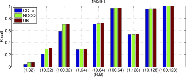 (b)
(b) 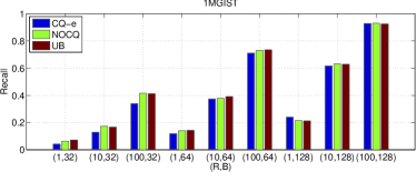
Product quantization and Cartesian -means. Product quantization [16] decomposes the space into low dimensional subspaces and quantizes each subspace separately. A vector is decomposed into subvectors, . Let the quantization dictionaries over the subspaces be with being a set of centers . A vector is represented by the concatenation of centers, , where is the one nearest to in the th quantization dictionary.
Rewrite each center as a -dimensional vector so that , i.e., all entries are zero except that the subvector corresponding to the th subspace is equal to . The approximation of a vector using the concatenation is then equivalent to the composition . Similarly, it can also be shown that there is a same equivalence in Cartesian -means [27].
The above analysis indicates that both product quantization and Cartesian -means can be regarded as a constrained version of composition quantization, with the orthogonality constraint: , , which guarantees that the near-orthogonality constraint in our approach holds. In addition, unlike product quantization and Cartesian -means in which each dictionary (subspace) is formed by dimensions, near-orthogonal composite quantization when , i.e., orthogonal composite quantization is able to automatically decide how many dimensions belong to one dictionary.
One may have a question: Is near-orthogonal composite quantization equivalent to product quantization over linearly transformed vectors and with proper choices of the number of dimensions in each subspace (dictionary)? The answer is NO. NOCQ does not transform data vectors, but relaxes the space spanned by the dictionary with a near-orthogonality constraint instead of orthogonality constraint.
| #Bits | Methods | SIFT | GIST |
|---|---|---|---|
| 32 | CQ | ||
| NOCQ | |||
| 64 | CQ | ||
| NOCQ | |||
| 128 | CQ | ||
| NOCQ |
Near-orthogonality constraint. The near-orthogonality constraint (10) is introduced to accelerate the search process. Table III shows that introducing this constraint results in higher quantization errors. One question comes: can we have alternative search process acceleration scheme if we learn the dictionaries using composite quantization without such a constraint to improve the approximation quality? We consider two possible schemes: when computing the distances in the search stage by (1) simply discarding the third term in Equation (8) or (2) precomputing and storing it as an extra code.
| Dataset | #Bits | Methods | Recall@1 | Recall@10 | Recall@100 |
| SIFT | 32, 32 | CQ | 0.110 | 0.374 | 0.775 |
| 32, 0 | CQ-d | 0.028 | 0.129 | 0.417 | |
| 32, 0 | NOCQ | 0.073 | 0.295 | 0.704 | |
| 64, 32 | CQ | 0.337 | 0.769 | 0.984 | |
| 64, 0 | CQ-d | 0.117 | 0.388 | 0.753 | |
| 32, 32 | CQ-c | 0.110 | 0.374 | 0.775 | |
| 64, 0 | NOCQ | 0.290 | 0.715 | 0.970 | |
| 128, 32 | CQ | 0.566 | 0.968 | 1.000 | |
| 128, 0 | CQ-d | 0.195 | 0.520 | 0.856 | |
| 96, 32 | CQ-c | 0.463 | 0.909 | 0.999 | |
| 128, 0 | NOCQ | 0.540 | 0.957 | 1.000 | |
| GIST | 32, 32 | CQ | 0.063 | 0.181 | 0.454 |
| 32, 0 | CQ-d | 0 | 0.002 | 0.006 | |
| 32, 0 | NOCQ | 0.064 | 0.173 | 0.416 | |
| 64, 32 | CQ | 0.131 | 0.380 | 0.742 | |
| 64, 0 | CQ-d | 0 | 0.003 | 0.007 | |
| 32, 32 | CQ-c | 0.063 | 0.181 | 0.454 | |
| 64, 0 | NOCQ | 0.140 | 0.378 | 0.730 | |
| 128, 32 | CQ | 0.232 | 0.628 | 0.948 | |
| 128, 0 | CQ-d | 0.027 | 0.080 | 0.226 | |
| 96, 32 | CQ-c | 0.205 | 0.524 | 0.876 | |
| 128, 0 | NOCQ | 0.215 | 0.631 | 0.930 |
Table IV shows the results of the two alternative schemes. We use our optimization algorithm to learn the CQ model, and the search performance of CQ is obtained by using extra bytes to store the value of the third term or equivalently taking higher search cost to compute the third term in the search stage. We have two observations: (1) Discarding the third term, denoted by CQ-d, leads to dramatic search quality reduction; (2) As expected, our approach NOCQ gets lower search performance than CQ, but higher than CQ-d (the third term discarded). It should be noted that CQ uses extra bytes or much higher search cost.
For fair comparison, we report the performance of CQ with the total code size consisting of both the bytes encoding the data vector and the extra bytes ( bits) encoding the third term. We can see that our approach performs much better.
From the Euclidean distance to the inner product. The Euclidean distance between the query and the vector can be transformed to an inner product form,
| (15) |
This suggests that in the search stage computing the second term is enough and thus we can quantize the augmented data vector, . It is shown in [5] that the inner product computation can also benefit from table lookup and thus is efficient. We report the performances of quantizing the augmented vector with the CQ approach, which performs better than PQ and CKM. The results are given in Table V. We can see that such a scheme performs poorly. It is because the scale of the last element is very different from the scales of other elements, and thus the optimization is hard. The possible solution of quantizing and separately also does not lead to much improvement, implying this is not a good direction.
The Euclidean distance between a query and the approximated vector can also be transformed to an inner product form, . Thus, similar to quantizing the third term in Equation (8), we can quantize the square of the norm, . The two quantization ways empirically show almost the same performance. The reason might be that the two terms are very close: .
| Dataset | #Bits | Methods | Recall@1 | Recall@10 | Recall@100 |
|---|---|---|---|---|---|
| SIFT | 32 | QAV | 0.018 | 0.099 | 0.339 |
| NOCQ | 0.073 | 0.295 | 0.704 | ||
| 64 | QAV | 0.103 | 0.355 | 0.731 | |
| NOCQ | 0.290 | 0.715 | 0.970 | ||
| 128 | QAV | 0.275 | 0.704 | 0.966 | |
| NOCQ | 0.540 | 0.957 | 1.000 | ||
| GIST | 32 | QAV | 0.016 | 0.102 | 0.304 |
| NOCQ | 0.064 | 0.173 | 0.416 | ||
| 64 | QAV | 0.059 | 0.248 | 0.581 | |
| NOCQ | 0.140 | 0.378 | 0.730 | ||
| 128 | QAV | 0.164 | 0.457 | 0.842 | |
| NOCQ | 0.215 | 0.631 | 0.930 |
6 Optimization
The formulation of near-orthogonal composite quantization is given as follows,
| (16) | ||||
| (17) | ||||
Here, is a matrix of size , and each column corresponds to an element of the th dictionary . is the composition vector, and its subvector is an indicator vector with only one entry being and all others being , showing which element is selected from the th dictionary to compose vector .
The problem formulated above is a mixed-binary-integer program, which consists of three groups of unknown variables: dictionaries , composition vectors , and . In addition to the binary-integer constraint over , there are near-orthogonality constraints over given in (17).
6.1 Algorithm
To handle the near-orthogonality constraint, we propose to adopt the quadratic penalty method, and add a penalty function that measures the violation of the quadratic equality constraints into the objective function, resulting in the following objective function,
| (18) | ||||
| (19) |
where and is the penalty parameter. The main technique we used is the alternative optimization method, where each step updates one variable while fixing the others.
Update . It can be easily seen that , the composition indicator of a vector , given fixed, is independent to all the other vectors . Then the optimization problem (18) is decomposed into subproblems,
| (20) |
where there are three constraints: is a binary vector, , and . Generally, this optimization problem is NP-hard. We notice that the problem is essentially a high-order MRF (Markov random field) problem. We again use the alternative optimization technique like the iterated conditional modes algorithm that is widely used to solve MRFs, and solve the subvectors alternatively. Given fixed, we update by exhaustively checking all the elements in the dictionary , finding the element such that the objective value is minimized, and accordingly setting the corresponding entry of to be and all the others to be . This process is iterated several ( in our implementation) times. The optimization is similar for solving composite quantization and orthogonal composite quantization.
Update . With and fixed, it can be shown that the optimal solution is
| (21) |
Update . Fixing and , the problem is an unconstrained nonlinear optimization problem with respect to . There are many algorithms for such a problem. We choose the quasi-Newton algorithm and specifically the L-BFGS algorithm, the limited-memory version of the Broyden-Fletcher-Goldfarb-Shanno (BFGS) algorithm. It only needs a few vectors to represent the approximation of the Hessian matrix instead of storing the full Hessian matrix as done in the BFGS algorithm. We adopt the publicly available implementation of L-BFGS333http://www.ece.northwestern.edu/~nocedal/lbfgs.html. The partial-derivative with respect to , the input to the L-BFGS solver, is computed as follows,
| (22) | ||||
| (23) |
In the case of composite quantization, there is a closed-form solution: , where is a matrix with each column corresponding to a database vector, and is a matrix composed of the composition vectors of all the database vectors, . In our implementation, we also adopt the iterative solution for composite quantization because we found that the iterative solution performs better. The optimization for orthogonal composite quantization is similar to that for near-orthogonal composite quantization with slight difference on the penalty part which is .
6.2 Implementation Details
The proposed algorithm is warm-started by using the solution of product quantization. There is a penalty parameter, , for the near-orthogonality constraint and the orthogonality constraint. Usually the penalty method needs to solve a series of unconstrained problems by increasing the penalty parameter into infinity to make the constraint completely satisfied. In our case, we find that the near-orthogonality term is not necessarily to be exactly constant and the search performance is still satisfactory if the deviation of the near-orthogonality term from a constant is relatively small compared with the quantization error. Therefore, our algorithm instead relaxes this constraint and selects the parameter via validation. The validation dataset is a subset of the database (selecting a subset is only for validation efficiency, and it is fine that the validation set is a subset of the learning set as the validation criterion is not the objective function value but the search performance). The best parameter is chosen so that the average search performance by regarding the validation vectors as queries and finding nearest neighbors from all the database vectors is the best.
6.3 Analysis
Complexity. We present the time complexity of each iteration. At the beginning of each iteration, we first compute inner product tables, , between the dictionary elements, taking , so that computing can be completed by one table lookup. The time complexities of the three updates are given as follows.
-
•
It takes with being the number of iterations ( in our implementation achieving satisfactory results) to update , i.e., optimize the objective function in (20), and thus the time complexity of updating is .
-
•
It takes to update , which can be easily seen from Equation (21).
-
•
The main cost of updating in near-orthogonal composite quantization lies in computing the partial derivatives and the objective function value that are necessary in L-BFGS. For clarity, we drop the complexity terms that are independent of and can be neglected for a large . Then, the time complexity for updating is with being the number of iterations ( in our implementation in average) and (set to in our implementation) being the number of line searches in L-BFGS.
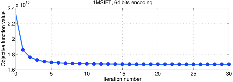
Convergence. The objective function value at each iteration in the algorithm always weakly decreases. It can be validated that the objective function value is lower-bounded (not smaller than ). The two points indicate the convergence of our algorithm. The theoretic analysis of the rate of convergence is not easy, while the empirical results show that the algorithm takes a few iterations to converge. Figure 4 shows an example convergence curve for near-orthogonal composite quantization.
7 Experiments
7.1 Setup
Datasets. We demonstrate the performance over six datasets (with scale ranged from small to large): MNIST444http://yann.lecun.com/exdb/mnist/ [22], grayscale images of handwritten digits; LabelMe [30], a corpus of images expressed as GIST descriptors; SIFT [16], consisting of SIFT features as base vectors, learning vectors and queries; GIST [16], containing global GIST descriptors as base vectors, learning vectors and queries; CNN [29], with convolution neural network (CNN) features as base vectors , CNN features as queries, extracted over the ImageNet training and test images through AlexNet [21]; and SIFT [18], composed of SIFT features as base vectors, learning vectors and queries. The details of the datasets are presented in Table VI.
Compared methods. We compare our approach, near-orthogonality composite quantization (NOCQ) with several state-of-the-art methods: product quantization (PQ) [16], and Cartesian -means (CKM) [27]. It is already shown that PQ and CKM achieve better search accuracy than hashing algorithms with the same code length and comparable search efficiency. Thus, we report one result from a representative hashing algorithm, iterative quantization (ITQ) [9]. All the results were obtained with the implementations generously provided by their respective authors. Following [16], we use the structured ordering for GIST and the natural ordering for SIFT and SIFT to get the best performance for PQ. We choose as the dictionary size which is an attractive choice because the resulting distance lookup tables are small and each subindex fits into one byte [16, 27].
Evaluation. To find ANNs, all the algorithms use asymmetric distance (i.e., query is not encoded) unless otherwise stated. To compare a query with a database vector, PQ, CKM and NOCQ conduct a few distance table lookups and additions, and ITQ uses asymmetric hamming distance for better search accuracy proposed in [11]. PQ, CKM, and NOCQ takes the same time for linear scan. Their costs of computing the distance lookup table are slightly different and are negligible when handling a large scale dataset, except the scale is small which is handled in our work [43]. For instance, the cost of computing the distance lookup table in our approach takes around of the cost of linear scan on SIFT. Figure 2 shows the average query times on SIFT and GIST, which shows the time costs are similar.
The search quality is evaluated using two measures: recall and mean average precision (MAP). Recall is defined as follows: for each query, we retrieve its nearest items and compute the ratio of to , i.e., the fraction of ground-truth nearest neighbors are found in the retrieved items. The average recall score over all the queries is used as the measure. The ground-truth nearest neighbors are computed over the original features using linear scan. In the experiments, we report the performance with being , , and . The MAP score is reported by regarding the nearest ground-truth neighbors as relevant answers to the query. The average precision for a query is computed as , where is the precision at cut-off in the ranked list and is the change in recall from items to . We report the mean of average precisions over all the queries under different code lengths.
(a) 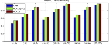 (b)
(b) 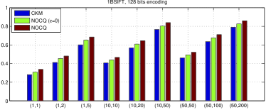
7.2 Empirical analysis
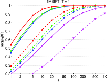
The effect of . The near-orthogonality variable in our approach is learnt from the reference base. Alternatively, one can simply set it to be zero, , indicating that the dictionaries are mutually orthogonal like splitting the spaces into subspaces as done in product quantization and Cartesian -means. The average quantization error in the case of learning potentially can be smaller than that in the case of letting as learning is more flexible, and thus the search performance with learnt can be better. The experimental results over the SIFT and SIFT dataset under the two schemes, shown in Figure 5. It can be seen that the performance when is not limited to be zero over SIFT is similar but much better over SIFT.


(a) 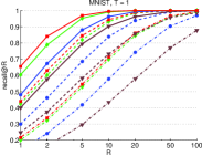
 (b)
(b) 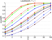

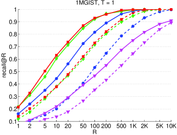
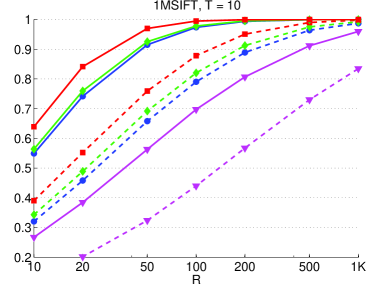
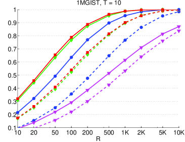
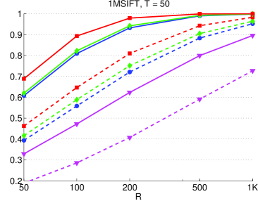

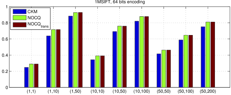
The effect of a global translation. One potential extension of our approach is to introduce an offset, denoted as , to translate . Introducing the offset does not increase the storage cost as it is a global parameter. The objective function with such an offset is as follows: . Our experiments indicate that this introduction does not influence the performance too much. An example result on SIFT with bits is shown in Figure 6. The reason might be that the contribution of the offset to the quantization distortion reduction is relatively small compared with that from the composition of selected dictionary elements.

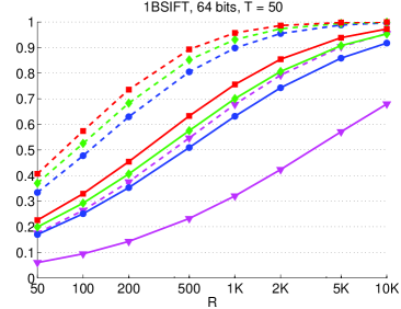
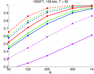
7.3 Comparison
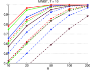
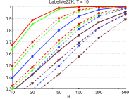
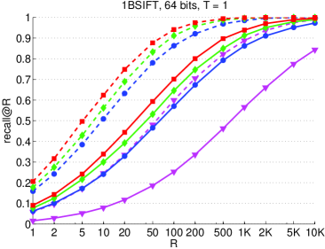
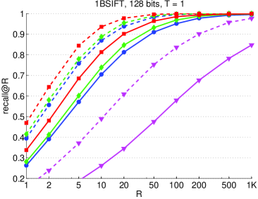
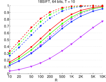
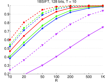
Recall@R. Figure 7 shows the comparison on MNIST and LabelMe. One can see that the vector approximation algorithms, our approach (NOCQ), CKM, and PQ, outperform ITQ. It is as expected because the information loss in Hamming embedding used in ITQ is much larger. PQ also performs not so good because it does not well exploit the data information for subspace partitioning. Our approach (NOCQ) is superior over CKM, and performs the best. The improvement seems a little small, but it is actually significant as the datasets are relatively small and the search is relatively easy.
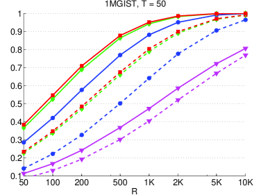
Figure 8 shows the results of large scale datasets: SIFT and GIST, using codes of bits and bits for searching , , and nearest neighbors. It can be seen that the gain obtained by our approach is significant for SIFT. For example, the recall with and bits for our approach is , about better than the recall of PQ, and larger than the recall of CKM. The reason of the relatively small improvement on GIST for NOCQ over CKM might be that CKM already achieves very large improvement over product quantization and the improvement space is relatively small.
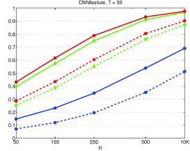
Figure 9 shows the performance on another large dataset, CNN, of a higher dimension. We use dataset vectors randomly sampled from the base set for efficient training. We do not show the ITQ results because ITQ performs much lower than PQ. It can be seen that our approach (NOCQ) outperforms PQ and CKM with both bits and bits encoding. For example, the recall for our approach with and bits is , about better than the recall of CKM, which is , and about better than the recall of PQ, which is . With bits encoding and , the recall of our approach is , about better than the recall of CKM and better than the recall of PQ. Note that CKM outperforms PQ significantly, which indicates that space partition is very important for CNN dataset. Our approach, on the other hand, still gets large improvement over CKM due to the more accurate data approximation.
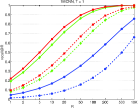
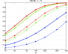
Figure 10 shows the performance for a very large dataset, SIFT. Similar to [27], we use the first learning vectors for efficient training. It can be seen that our approach, NOCQ, gets the best performance and the improvement is consistently significant. For example, the recall from our approach on the base set with bits for is while from CKM it is . Besides the performance over all the database vectors, we also show the performance on a subset of base vectors, the first database vectors. As we can see, the performance on vectors is worse than that on vectors, which is reasonable as searching over a larger dataset is more difficult. The notable observation is that the improvement of our approach over Cartesian -means on the larger dataset, database vectors, is much more significant than that on database vectors.
(a)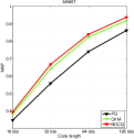 (b)
(b)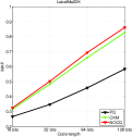 (c)
(c)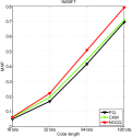 (d)
(d)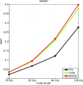 (e)
(e)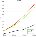 (f)
(f)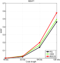
MAP vs. #bits. Figure 11 shows the MAP performance on (a) MNIST, (b) LabelMe. (c) SIFT, (d) GIST, (e) CNN and (f) SIFT with various code lengths. We can see that our approach (NOCQ) performs the best on all the datasets. It is worth noting that the improvement obtained on SIFT is significant since searching in 1 billion vectors is not easy. For instance, the MAP scores of SIFT on 64 bits for NOCQ and PQ are and , and the relative improvement is about . The MAP scores for NOCQ and CKM are and , and the improvement reaches .
8 Applications
8.1 Inverted Multi-Index
Inverted multi-index [3] performs product quantization on the database vectors to generate the cell centroids which store the list of vectors that lie in a cluster. The multi-sequence algorithm [3] is introduced to efficiently produce a sequence of multi-index cells ordered by the increasing distances between the query and the cell centroids, with the aim of retrieving the NN candidates. After that, the retrieved candidates are often reranked based on their short codes, e.g., through product quantization [18]. We follow the Multi-D-ADC scheme [3], which, in the reranking stage, apply the compact coding algorithm to the residual displacement between each vector and its closest cell centroids obtained through the indexing stage.
All the compared methods can be applied to build inverted multi-index (coarse quantization used in the candidate retrieval stage) and compact code representation (fine quantization used in the reranking stage). On the candidate retrieval stage, the distance table between the query and the coarse codebooks is computed before performing the multi-sequence algorithm for candidate retrieval. On the reranking stage, there are two ways for distance computation: with reconstructing the database vector, and without reconstructing the database vector but through looking up distance tables like [4]. Here we show how to accelerate the distance computation without reconstructing the database vector in our approach.
Efficient distance computation. We adopt two dictionaries and , suggested by [4] for coarse quantization, and represent the dictionaries for fine quantization by . Let the approximation of a vector be . The acceleration idea is inspired by [4], and illustrated below. Expanding the approximated distance computation,
| (24) | ||||
| (25) |
we can see that the right-hand-side contains terms. The first term only depends on the query, and is not necessary to compute. The second and the third terms are the summation of the norms of the selected quantization centers, where the norms are offline computed, and hence the complexity is . In the fourth term the inner products have been computed in the candidate retrieval stage, and this complexity is . The fifth term takes time if the inner products between the query and the dictionary elements for the fine quantizer are precomputed. The sixth term takes when the inner products between the elements of the coarse and fine dictionaries are precomputed offline. The last two terms are omitted because they are approximately equal to a constant (the constant equals 0 for PQ and CKM). In summary, the online time complexity is with precomputing the inner product table storing the inner products between the query and the fine dictionary elements.
| Alg. | ||||||
|---|---|---|---|---|---|---|
| BIGANN, 1 billion SIFTs, bits per vector | ||||||
| PQ | ||||||
| CKM | ||||||
| NOCQ | ||||||
| SNOCQ1 | ||||||
| SNOCQ2 | ||||||
| PQ | ||||||
| CKM | ||||||
| NOCQ | ||||||
| SNOCQ1 | ||||||
| SNOCQ2 | ||||||
| PQ | ||||||
| CKM | ||||||
| NOCQ | ||||||
| SNOCQ1 | ||||||
| SNOCQ2 | ||||||
| BIGANN, 1 billion SIFTs, bits per vector | ||||||
| PQ | ||||||
| CKM | ||||||
| NOCQ | ||||||
| SNOCQ1 | ||||||
| SNOCQ2 | ||||||
| PQ | ||||||
| CKM | ||||||
| NOCQ | ||||||
| SNOCQ1 | ||||||
| SNOCQ2 | ||||||
| PQ | ||||||
| CKM | ||||||
| NOCQ | ||||||
| SNOCQ1 | ||||||
| SNOCQ2 | ||||||
Results. We compare the proposed approach, NOCQ, with PQ and CKM, and use them to train the coarse and fine quantizers. In addition, we also report the results of the sparse version of our approach [43]: the dictionary is sparse, thus the distance table computation is accelerated. We consider two sparsity degrees: one, termed as SNOCQ1, has the same sparse degree (i.e., the number of nonzeros ) with PQ, and the other, SNOCQ2, in which the number of nonzeros is equal to , has similar distance table computation cost with CKM. Following [3], for all the approaches, we use to build coarse dictionaries and for compact code representation. The performance comparison in terms of recall (), (query time cost for the scheme with database vector reconstruction), (query time cost for the scheme without database vector reconstruction but through distance lookup tables) with respect to the length of the retrieved candidate list () is summarized in Table VII.
It can be seen in terms of the search accuracy that our approach NOCQ performs the best and that our approach SNOCQ1 (SNOCQ2) performs better than PQ (CKM). Compared with the and columns, our approaches, SNOCQ1 and SNOCQ2, like PQ and CKM, are both accelerated, and according to the column, the query costs of our approaches (SNOCQ1 and SNOCQ2) are almost the same to that of the most efficient approach PQ. Considering the overall performance in terms of the query cost for the accelerated scheme () and the recall, one can see that SNOCQ2 performs the best. For example, the query cost of SNOCQ2 is smaller than that of NOCQ when retrieving candidates with bits and the recall decreases less than . In other cases, the recall decrease is always less than while the query cost is saved at least . In summary, our approach NOCQ is the best choice if the code length, thus storage and memory cost, is top priority, or if a larger number of candidate images are needed to rerank, and its sparse version performs the best when concerning about both query time and storage cost.
8.2 Inner Product Similarity Search
In this section, we study the application of composite quantization to maximum inner product similarity search, which aims to find a database vector so that . Given the approximation , the approximated inner product between a query and a database vector is computed by . The computation cost can be reduced to by looking up an inner product table storing inner products, .
Similar to the triangle inequality for upper-bounding the Euclidean distance approximation error, we have a property for the inner product distance approximation error, and the property is given as,
Property 3.
Given a query vector , a data vector and its approximation , the absolute difference between the true inner product and the approximated inner product is upper-bounded:
| (26) |
The upper bound is related to the norms of , meaning that the bound depends on the query (in contrast, the upper bound for Euclidean distance does not depend on the query). However, the solution in inner product similarity search does not depend on the norm of the query as queries with different norm have the same solution, i.e., , where is an arbitrary positive number. In this sense, it also holds that more accurate vector approximation can potentially lead to better inner product similarity search.
The results of different algorithms over SIFT, GIST and SIFT are shown in Figure 12. The groundtruth nearest neighbors of a given query are computed by linear scanning all the database vectors and evaluating the inner product similarity between the query and each database vector. We can see that our approach gets the best performance on all the datasets with various code lengths.

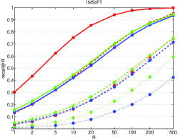
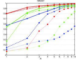
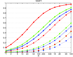
8.3 Query Compression for Mobile Search
Mobile search is an emerging direction of image and information retrieval. It is usually expected that the object transmitted from the client to the server is as small as possible. In this section, we conduct an experiment: the database points are processed using the compact coding approach, e.g., NOCQ, PQ and CKM; the query is transformed to a compact code (in the client side); the query reconstructed (in the server side) from the transformed compact code is compared with the database points. The query is compressed in our approach NOCQ using the non-orthogonal version CQ as the reconstruction quality is better, while the same coding scheme is used in both the client and server sides for other approaches.
The results are shown in Figure 13 over SIFT, GIST, and SIFT (its whole data is used as the search database) with bits and bits for -NN search. It is as expected that our approach consistently performs the best. In particularly, the improvement gain of our approach over the second best method, CKM, is even more signification compared with the results shown in Figures 8 and 10 obtained without compressing the query. For example, the recall gain for SIFT with bits at position is increased from to , and the recall gain for SIFT with bits at position is increased from to .

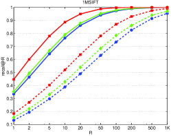
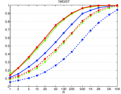
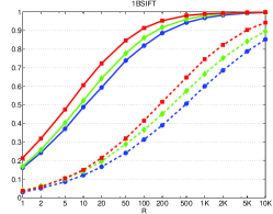
| Bits | ITQ | PQ | CKM | NOCQ | |
|---|---|---|---|---|---|
| Fisher | |||||
| VLAD | |||||
| Bits | ITQ | PQ | CKM | NOCQ | |
|---|---|---|---|---|---|
| Fisher | |||||
| VLAD | |||||
8.4 Application to object retrieval
We report the results of the applications to object retrieval. In object retrieval, images are represented as an aggregation of local descriptors, often thousands of dimension. We evaluate the performances over the -dimensional Fisher vectors [28] and the -dimensional VLAD vectors [17] extracted from the INRIA Holidays dataset [15] that contains query and relevant images, and the UKBench dataset [26] that contains groups of images each (totally images).
9 Conclusion
In this paper, we present a compact coding approach, near-orthogonal composite quantization, to approximate nearest neighbor search. The superior search accuracy stems from that it exploits the composition of dictionary elements to approximate a vector, yielding smaller quantization errors. The search efficiency is guaranteed by imposing the near-orthogonality constraint and discarding its computation. The empirical results suggest that near-orthogonal composite quantization outperforms existing methods for search under the Euclidean-distance and composite quantization achieves superior performance for search with the inner-product similarity. Composite quantization has been extended to semantic quantization [38] for semantic retrieval and multi-modality quantization [44] for multi-modality search.
Appendix: Proof of Theorem 2
Proof.
We have the following inequality,
| (27) |
We will show (a) and (b) , respectively.
The proof for (a) is given as follows,
| (28) | ||||
| (29) |
The proof for (b) is presented in the following. For convenience, we denote .
| (30) |
We can easily validate (b) in the case that the denominator happens to be in the above proof.
Thus, the theorem holds. ∎
Appendix: Proof of Property 3
Proof.
The proof is simple and given as follows. Look at the absolute value of the inner product approximation error,
| (31) | ||||
| (32) | ||||
| (33) | ||||
| (34) |
Thus, the approximation error is upper-bounded by , assuming that is upper-bounded by a constant . ∎
References
- [1] A. Babenko and V. Lempitsky. Additive quantization for extreme vector compression. In CVPR, pages 931–939, 2014.
- [2] A. Babenko and V. Lempitsky. Tree quantization for large-scale similarity search and classification. In CVPR, 2015.
- [3] A. Babenko and V. S. Lempitsky. The inverted multi-index. In CVPR, pages 3069–3076, 2012.
- [4] A. Babenko and V. S. Lempitsky. Improving bilayer product quantization for billion-scale approximate nearest neighbors in high dimensions. CoRR, abs/1404.1831, 2014.
- [5] C. Du and J. Wang. Inner product similarity search using compositional codes. CoRR, abs/1406.4966, 2014.
- [6] J. H. Friedman, J. L. Bentley, and R. A. Finkel. An algorithm for finding best matches in logarithmic expected time. ACM Trans. Math. Softw., 3(3):209–226, 1977.
- [7] T. Ge, K. He, Q. Ke, and J. Sun. Optimized product quantization for approximate nearest neighbor search. In CVPR, pages 2946–2953, 2013.
- [8] Y. Gong, S. Kumar, V. Verma, and S. Lazebnik. Angular quantization-based binary codes for fast similarity search. In NIPS, pages 1205–1213, 2012.
- [9] Y. Gong and S. Lazebnik. Iterative quantization: A procrustean approach to learning binary codes. In CVPR, pages 817–824, 2011.
- [10] Y. Gong, S. Lazebnik, A. Gordo, and F. Perronnin. Iterative quantization: A procrustean approach to learning binary codes for large-scale image retrieval. IEEE Trans. Pattern Anal. Mach. Intell., 35(12):2916–2929, 2013.
- [11] A. Gordo and F. Perronnin. Asymmetric distances for binary embeddings. In CVPR, pages 729–736, 2011.
- [12] A. Gordo, F. Perronnin, Y. Gong, and S. Lazebnik. Asymmetric distances for binary embeddings. IEEE Trans. Pattern Anal. Mach. Intell., 36(1):33–47, 2014.
- [13] R. M. Gray and D. L. Neuhoff. Quantization. IEEE Transactions on Information Theory, 44(6):2325–2383, 1998.
- [14] J.-P. Heo, Z. Lin, and S.-E. Yoon. Distance encoded product quantization. In CVPR, pages 2139–2146, 2014.
- [15] H. Jegou, M. Douze, and C. Schmid. Hamming embedding and weak geometric consistency for large scale image search. In ECCV, pages 304–317, 2008.
- [16] H. Jégou, M. Douze, and C. Schmid. Product quantization for nearest neighbor search. IEEE Trans. Pattern Anal. Mach. Intell., 33(1):117–128, 2011.
- [17] H. Jégou, M. Douze, C. Schmid, and P. Pérez. Aggregating local descriptors into a compact image representation. In CVPR, pages 3304–3311, 2010.
- [18] H. Jégou, R. Tavenard, M. Douze, and L. Amsaleg. Searching in one billion vectors: Re-rank with source coding. In ICASSP, pages 861–864, 2011.
- [19] Y. Kalantidis and Y. Avrithis. Locally optimized product quantization for approximate nearest neighbor search. In CVPR, pages 2329–2336, 2014.
- [20] W. Kong and W.-J. Li. Isotropic hashing. In NIPS, pages 1655–1663, 2012.
- [21] A. Krizhevsky, I. Sutskever, and G. E. Hinton. Imagenet classification with deep convolutional neural networks. In Advances in Neural Information Processing Systems 25: 26th Annual Conference on Neural Information Processing Systems 2012. Proceedings of a meeting held December 3-6, 2012, Lake Tahoe, Nevada, United States., pages 1106–1114, 2012.
- [22] Y. LeCun, L. Bottou, Y. Bengio, and P. Haffner. Gradient-based learning applied to document recognition. In Intelligent Signal Processing, pages 306–351. IEEE Press, 2001.
- [23] W. Liu, J. Wang, R. Ji, Y.-G. Jiang, and S.-F. Chang. Supervised hashing with kernels. In CVPR, pages 2074–2081, 2012.
- [24] Y. Matsui, T. Yamasaki, and K. Aizawa. Pqtable: Fast exact asymmetric distance neighbor search for product quantization using hash tables. 2015.
- [25] M. Muja and D. G. Lowe. Fast approximate nearest neighbors with automatic algorithm configuration. In VISSAPP (1), pages 331–340, 2009.
- [26] D. Nistér and H. Stewénius. Scalable recognition with a vocabulary tree. In CVPR (2), pages 2161–2168, 2006.
- [27] M. Norouzi and D. J. Fleet. Cartesian k-means. In CVPR, pages 3017–3024, 2013.
- [28] F. Perronnin and C. R. Dance. Fisher kernels on visual vocabularies for image categorization. In CVPR, 2007.
- [29] O. Russakovsky, J. Deng, H. Su, J. Krause, S. Satheesh, S. Ma, Z. Huang, A. Karpathy, A. Khosla, M. Bernstein, A. C. Berg, and L. Fei-Fei. Imagenet large scale visual recognition challenge. International Journal of Computer Vision (IJCV), pages 1–42, April 2015.
- [30] B. C. Russell, A. Torralba, K. P. Murphy, and W. T. Freeman. Labelme: A database and web-based tool for image annotation. International Journal of Computer Vision, 77(1-3):157–173, 2008.
- [31] G. Shakhnarovich, T. Darrell, and P. Indyk. Nearest-Neighbor Methods in Learning and Vision: Theory and Practice. The MIT press, 2006.
- [32] C. Silpa-Anan and R. Hartley. Optimised kd-trees for fast image descriptor matching. In CVPR, 2008.
- [33] J. Wang, S. Kumar, and S.-F. Chang. Semi-supervised hashing for large-scale search. IEEE Trans. Pattern Anal. Mach. Intell., 34(12):2393–2406, 2012.
- [34] J. Wang and S. Li. Query-driven iterated neighborhood graph search for large scale indexing. In ACM Multimedia, pages 179–188, 2012.
- [35] J. Wang, H. T. Shen, J. Song, and J. Ji. Hashing for similarity search: A survey. CoRR, abs/1408.2927, 2014.
- [36] J. Wang, J. Wang, J. Song, X.-S. Xu, H. T. Shen, and S. Li. Optimized cartesian -means. CoRR, abs/1405.4054, 2014.
- [37] J. Wang, T. Zhang, J. Song, N. Sebe, and H. T. Shen. A survey on learning to hash. CoRR, abs/1606.00185, 2016.
- [38] X. Wang, T. Zhang, G.-J. Qi, J. Tang, and J. Wang. Supervised quantization for similarity search. In CVPR, pages 2018–2026, 2016.
- [39] B. Xu, J. Bu, Y. Lin, C. Chen, X. He, and D. Cai. Harmonious hashing. In IJCAI, 2013.
- [40] F. Yu, S. Kumar, Y. Gong, and S.-F. Chang. Circulant binary embedding. In ICML (2), pages 946–954, 2014.
- [41] M. Yuan and Y. Lin. Model selection and estimation in regression with grouped variables. Journal of the Royal Statistical Society, Series B, 68:49–67, 2006.
- [42] T. Zhang, C. Du, and J. Wang. Composite quantization for approximate nearest neighbor search. In ICML (2), pages 838–846, 2014.
- [43] T. Zhang, G.-J. Qi, J. Tang, and J. Wang. Sparse composite quantization. In CVPR, pages 4548–4556, 2015.
- [44] T. Zhang and J. Wang. Collaborative quantization for cross-modal similarity search. In CVPR, pages 2036–2045, 2016.