A Stable SPH Discretization of the Elliptic Operator with Heterogeneous Coefficients

Alexander A. Lukyanov  and  Kees Vuik
Abstract.

Smoothed particle hydrodynamics (SPH) has been extensively used to model high and low Reynolds number flows, free surface flows and collapse of dams, study pore-scale flow and dispersion, elasticity, and thermal problems. In different applications, it is required to have a stable and accurate discretization of the elliptic operator with homogeneous and heterogeneous coefficients. In this paper, the stability and approximation analysis of different SPH discretization schemes (traditional and new) of the diagonal elliptic operator for homogeneous and heterogeneous media are presented. The optimum and new discretization scheme is also proposed. This scheme enhances the Laplace approximation (Brookshaw’s scheme [1] and Schwaiger’s scheme [2]) used in the SPH community for thermal, viscous, and pressure projection problems with an isotropic elliptic operator. The numerical results are illustrated by numerical examples, where the comparison between different versions of the meshless discretization methods are presented.

Key words and phrases:
Meshless method, Stability and Approximation, Laplace operator, Diffusive flow, Monotone scheme, Discrete maximum principle
2010 Mathematics Subject Classification:
97N40, 65N75, 76M28
Delft University of Technology, Faculty of Electrical Engineering, Mathematics and Computer Science, Delft Institute of Applied Mathematics, 2628CN Delft, the Netherlands (aalukyanov1@gmail.com, c.vuik@tudelft.nl).

1. Introduction

Smoothed particle hydrodynamics (SPH) was developed a few decades ago to model inviscid fluid and gas flow dynamics in astrophysical problems [3, 4, 5, 6]. The SPH is an interpolation-based numerical technique that can be used to solve systems of partial differential equations (PDEs) using either Lagrangian or Eulerian descriptions. The nature of SPH method allows to incorporate different physical and chemical effects into the discretized governing equations with relatively small code-development effort. In addition, geometrically complex and/or dynamic boundaries, and interfaces can be handled without undue difficulty. The SPH numerical procedure of calculating state variables (i.e., density, velocity, and gradient of deformation) are computed as a weighted average of values in a local region. Despite a few advantages of SPH method, this method is not free from disadvantages. For example, for fluids, gases, or solids with non-trivial boundaries there is incompleteness of the kernel support combined with the lack of consistency of the kernel interpolation in conventional meshless methods which results in fuzzy boundaries. In some cases, this can be fixed by an automatic incorporation of the boundary condition [3]. The completeness of mesh free particle methods was discussed in [7]. However, care must be taken to ensure that variables whose values do not approach zero at boundaries are accurately represented.

It has been observed in the literature that meshless methods (e.g., SPH) are not free from instabilities, especially in the modeling solid mechanics problems. For example, the tensile instabilities were identified in [8] by performing the Neumann analysis of the one-dimensional governing equations (conservation laws). Therefore, different stabilization techniques have been developed. It is important to note at this point that it is very difficult to perform the general Neumann analysis in two- and three-dimensions. Furthermore, the high-frequency instability results from the low order discretization (rank deficient) of the divergence operator. The tensile instability results from the interaction between the second derivative of the Eulerian kernel (i.e., computed kernel in the Eulerian coordinates) and the tensile stress. The tensile instability only occurs for the Eulerian kernels because the Eulerian kernels depend on both the stress and the second derivative of the kernel. It has been shown [9] that in the case where the kernel is a function of the Lagrangian coordinates (the Lagrangian kernel), tensile instability does not occur. A comprehensive analysis on this subject can be found in [9]. Recently, some regularization and stabilization of SPH schemes were proposed in [10], [11].

Since its introduction, SPH has been successfully used to model a wide range of fluid flows and the behavior of solids subjected to large deformations. For example, the SPH method was applied to simulate high energy explosions [12] and impact [13, 14], most notably free surface flows and collapse of dams [15], elastoplasticity [16, 17, 18, 14], to model low Reynolds number flows [19, 20], to study pore-scale flow and dispersion [21, 22], and for thermal problems [17, 23, 2].

In different applications including, but not limited to, fluid flow related problems, it is required to have the stable and accurate discretization of the following operator (diagonal elliptic operator), which is the research subject of this paper:

𝐋(𝐮)=(𝐌(𝒓)𝐮(𝒓))g(𝒓),𝒓Ωn,𝐌(𝒓){diag[m(𝒓)]:m(𝒓)+n,m(𝒓)L2(Ω)},diag:nn×n,formulae-sequence𝐋𝐮𝐌𝒓𝐮𝒓𝑔𝒓for-all𝒓Ωsuperscript𝑛missing-subexpressionmissing-subexpression:𝐌𝒓conditional-setdiagdelimited-[]𝑚𝒓formulae-sequence𝑚𝒓subscriptsuperscript𝑛𝑚𝒓subscript𝐿2Ωdiagsuperscript𝑛superscript𝑛𝑛missing-subexpressionmissing-subexpression\begin{array}[]{lcl}\displaystyle\vspace{0.2cm}\mathbf{L}\left(\mathbf{u}\right)=-\nabla\left(\mathbf{M}\left(\boldsymbol{r}\right)\nabla\mathbf{u}\left(\boldsymbol{r}\right)\right)-g\left(\boldsymbol{r}\right),\ \forall\boldsymbol{r}\in\Omega\subset\mathbb{R}^{n},\\ \mathbf{M}\left(\boldsymbol{r}\right)\in\{\mbox{diag}[m(\boldsymbol{r})]:m(\boldsymbol{r})\in\mathbb{R}^{n}_{+},\ m\left(\boldsymbol{r}\right)\in L_{2}\left(\Omega\right)\},\ \mbox{diag}:\mathbb{R}^{n}\rightarrow\mathbb{R}^{n\times n},\end{array} (1)

where 𝐮(𝒓)𝐮𝒓\mathbf{u}\left(\boldsymbol{r}\right) is the unknown scalar or vector variable field, 𝐌αβ(𝒓)superscript𝐌𝛼𝛽𝒓\mathbf{M}^{\alpha\beta}\left(\boldsymbol{r}\right) is the diagonal matrix of the mobility field, e.g., one example includes 𝐌αβ(𝒓)=m(𝒓)δαβ,α,β=1,,n;formulae-sequencesuperscript𝐌𝛼𝛽𝒓𝑚𝒓subscript𝛿𝛼𝛽𝛼𝛽1𝑛\mathbf{M}^{\alpha\beta}\left(\boldsymbol{r}\right)=m\left(\boldsymbol{r}\right)\delta_{\alpha\beta},\ \alpha,\beta=1,\ldots,n;, where m(𝒓)𝑚𝒓m\left(\boldsymbol{r}\right) is the mobility scalar field, δαβsubscript𝛿𝛼𝛽\delta_{\alpha\beta} is the Kronecker symbol, n=1,2,3𝑛123n=1,2,3 is the spatial dimension. The sink/source term g(𝒓)𝑔𝒓g\left(\boldsymbol{r}\right) is assumed to be zero in this paper. Consider the operator in the expression (1) with piecewise continuous coefficients 𝐌(𝒓)𝐌𝒓\mathbf{M}\left(\boldsymbol{r}\right) in ΩΩ\Omega. It has been noticed that some of the numerical methods for elliptic equations may violate the maximum principle (i.e. lead to spurious oscillations). Therefore, proposed methods must satisfy a discrete maximum principle to avoid any spurious oscillations. This is also applicable to meshless discretizations. Usually, the oscillations are closely related to the poor approximation of the variable gradient 𝐮𝐮\nabla\mathbf{u} in the flux computation. In this paper, different numerical discretizations of the elliptic isotropic operator are analyzed. The objective of this paper is to develop numerical scheme satisfying the two-point flux approximation nature in the form

𝐋(𝐮)JV𝒓JΨ([𝐮(𝒓J)𝐮(𝒓I)],𝒓J𝒓I)g(𝒓I),𝐋𝐮subscript𝐽subscript𝑉subscript𝒓𝐽Ψdelimited-[]𝐮subscript𝒓𝐽𝐮subscript𝒓𝐼subscript𝒓𝐽subscript𝒓𝐼𝑔subscript𝒓𝐼\displaystyle\mathbf{L}\left(\mathbf{u}\right)\approx\sum_{J}V_{\boldsymbol{r}_{J}}\Psi\left(\left[\mathbf{u}\left(\boldsymbol{r}_{J}\right)-\mathbf{u}\left(\boldsymbol{r}_{I}\right)\right],\boldsymbol{r}_{J}-\boldsymbol{r}_{I}\right)-g\left(\boldsymbol{r}_{I}\right), (2)

where J𝐽J is the neighboring particle of the particle I𝐼I, V𝒓Jsubscript𝑉subscript𝒓𝐽V_{\boldsymbol{r}_{J}} is the J𝐽J - particle volume, ΨΨ\Psi is the special kernel. This structure (2) allows to have a better analysis of the stability and monotonicity. Furthermore, this will allow to apply upwinding strategy during the solution of nonlinear PDEs. The optimum discretization scheme of the shape (2) is proposed in this paper. This scheme is based both on the Laplace approximation (Brookshaw’s scheme [1]) and on a gradient approximation commonly used in the SPH community for thermal, viscous, and pressure projection problems. The proposed discretization scheme is combined with mixed corrections, which ensure linear completeness. The mixed correction utilizes Shepard Functions in combination with a correction to derivative approximations. In corrected meshless methods, the domain boundaries and field variables at the boundaries are approximated with the improved accuracy comparing to the conventional SPH method. The resulting new scheme improves the particle deficiency (kernel support incompleteness) problem. The outline of the paper is as follows. In section 2, the existing discretizations of the Laplace operator with the building blocks necessary for these methods are discussed. In this section, the SPH kernel and its gradient properties are also discussed. The description of meshless transmisibilities and their connections to the existing mesh-dependent discretization schemes is given in section 3 including the construction of a new meshless discretization scheme. The approximation, stability, and monotonicity analysis are performed in section 4. The numerical analysis of different boundary value problems is presented in section 5. The paper is concluded by section 6.

2. SPH discretization of the Laplace operator

The meshless approximations (SPH approximations) to the operator (1) with heterogeneous and homogeneous coefficients are presented in this section. Let us consider a rectangle in n,n=1,2,3formulae-sequencesuperscript𝑛𝑛123\mathbb{R}^{n},\ n=1,2,3:

Ω={𝒓={xi}n| 0<|xiai|<li,li+,i=1,,n}Ωconditional-set𝒓subscript𝑥𝑖superscript𝑛formulae-sequence 0subscript𝑥𝑖subscript𝑎𝑖subscript𝑙𝑖formulae-sequencesubscript𝑙𝑖subscriptfor-all𝑖1𝑛\displaystyle\Omega=\left\{\boldsymbol{r}=\left\{x_{i}\right\}\in\mathbb{R}^{n}\left|\right.\ \ 0<\left|x_{i}-a_{i}\right|<l_{i},\ l_{i}\in\mathbb{R}_{+},\ \ \forall i=1,\ldots,n\right\} (3)

as the numerical domain. Here, aisubscript𝑎𝑖a_{i} are the center coordinates of the rectangular and lisubscript𝑙𝑖l_{i} are the side lengths. The following norms are used to quantify the accuracy of different approximations for the entire numerical domain ΩΩ\Omega:

𝐟Ω¯p=(𝝃kΩ¯V𝝃k(|𝐟|)p)1p,𝐟Ω~p=(𝝃kΩ~V𝝃k(|𝐟|)p)1pformulae-sequencesubscriptsuperscriptnorm𝐟𝑝¯Ωsuperscriptsubscriptsubscript𝝃𝑘¯Ωsubscript𝑉subscript𝝃𝑘superscript𝐟𝑝1𝑝subscriptsuperscriptnorm𝐟𝑝~Ωsuperscriptsubscriptsubscript𝝃𝑘~Ωsubscript𝑉subscript𝝃𝑘superscript𝐟𝑝1𝑝\displaystyle\left\|\mathbf{f}\right\|^{{p}}_{\bar{\Omega}}=\left(\sum\limits_{\boldsymbol{\xi}_{k}\in\bar{\Omega}}V_{\boldsymbol{\xi}_{k}}\left(\left|\mathbf{f}\right|\right)^{p}\right)^{\frac{1}{p}},\ \left\|\mathbf{f}\right\|^{{p}}_{\tilde{\Omega}}=\left(\sum\limits_{\boldsymbol{\xi}_{k}\in\tilde{\Omega}}V_{\boldsymbol{\xi}_{k}}\left(\left|\mathbf{f}\right|\right)^{p}\right)^{\frac{1}{p}} (4)

where 𝐟𝐟\mathbf{f} is the approximated physical quantity, V𝝃ksubscript𝑉subscript𝝃𝑘V_{\boldsymbol{\xi}_{k}} is the volume of the particle 𝝃ksubscript𝝃𝑘\boldsymbol{\xi}_{k}, Ω¯¯Ω\bar{\Omega} denotes entire domain including boundary particles, Ω~~Ω\tilde{\Omega} denotes only internal part of the domain ΩΩ{\Omega}.

The proposed discretization schemes should be compatible with a discontinuous m(𝒓)𝑚𝒓m\left(\boldsymbol{r}\right) (or piecewise function) coefficient of the operator (1) since this coefficient cannot be differentiable in the classical sense. The standard SPH spatial discretization of the Laplace operator (1) arises from the following relations (g(𝒓)=0,𝒓𝑔𝒓0for-all𝒓g\left(\boldsymbol{r}\right)=0,\ \forall\boldsymbol{r}):

𝐋(𝐮(𝒓I))=limh~I0Ω𝒓I,h~I𝐋(𝐮(𝒓))W(𝒓𝒓I,h~I)𝑑V𝒓limh~I0[Ω𝒓I,h~I𝐌(𝒓)𝐮(𝒓)W(𝒓𝒓I,h~I)𝑑V𝒓],delimited-⟨⟩𝐋𝐮subscript𝒓𝐼subscriptsubscript~𝐼0subscriptsubscriptΩsubscript𝒓𝐼subscript~𝐼𝐋𝐮𝒓𝑊𝒓subscript𝒓𝐼subscript~𝐼differential-dsubscript𝑉𝒓absentmissing-subexpressionmissing-subexpressionabsentsubscriptsubscript~𝐼0delimited-[]subscriptsubscriptΩsubscript𝒓𝐼subscript~𝐼𝐌𝒓𝐮𝒓𝑊𝒓subscript𝒓𝐼subscript~𝐼differential-dsubscript𝑉𝒓missing-subexpressionmissing-subexpression\begin{array}[]{lcl}\displaystyle\vspace{0.2cm}\langle\mathbf{L}\left(\mathbf{u}\left(\boldsymbol{r}_{I}\right)\right)\rangle=\lim\limits_{\tilde{h}_{I}\rightarrow 0}\int\limits_{\Omega_{\boldsymbol{r}_{I},\tilde{h}_{I}}}\mathbf{L}\left(\mathbf{u}\left(\boldsymbol{r}\right)\right)W\left(\boldsymbol{r}-\boldsymbol{r}_{I},\tilde{h}_{I}\right)dV_{\boldsymbol{r}}\approx\\ \displaystyle\approx\lim\limits_{\tilde{h}_{I}\rightarrow 0}\left[\int\limits_{\Omega_{\boldsymbol{r}_{I},\tilde{h}_{I}}}\mathbf{M}\left(\boldsymbol{r}\right)\nabla\mathbf{u}\left(\boldsymbol{r}\right)\cdot\nabla W\left(\boldsymbol{r}-\boldsymbol{r}_{I},\tilde{h}_{I}\right)dV_{\boldsymbol{r}}\right],\end{array} (5)

where W(𝒓𝒓I,h~I)𝑊𝒓subscript𝒓𝐼subscript~𝐼W\left(\boldsymbol{r}-\boldsymbol{r}_{I},\tilde{h}_{I}\right) is the kernel that weakly approximates the Dirac delta function δ(𝒓𝒓I)𝛿𝒓subscript𝒓𝐼\delta\left(\boldsymbol{r}-\boldsymbol{r}_{I}\right) but with finite characteristic width h~Isubscript~𝐼\tilde{h}_{I} around the particle I𝐼I. The effective characteristic width h~Isubscript~𝐼\tilde{h}_{I} will be defined in the upcoming section using real smoothing particle length hIsubscript𝐼h_{I}. However, it is important to note that, in the case of the homogeneous particle distribution, it is common to use h~I=fhp,f1formulae-sequencesubscript~𝐼𝑓subscript𝑝𝑓1\tilde{h}_{I}=f\cdot h_{p},\ f\geq 1, where hpsubscript𝑝h_{p} is the inter-particles distance. Hence, it is important that h~Isubscript~𝐼\tilde{h}_{I} and hpsubscript𝑝h_{p} are not mixed up during the analysis. The control volumes in the meshless discretization are the patches, which are interior to the support of the kernels W(𝒓𝒓I,h~I)𝑊𝒓subscript𝒓𝐼subscript~𝐼W\left(\boldsymbol{r}-\boldsymbol{r}_{I},\tilde{h}_{I}\right), i.e. Ω𝒓I,h~I=suppW(𝒓𝒓I,h~I)subscriptΩsubscript𝒓𝐼subscript~𝐼supp𝑊𝒓subscript𝒓𝐼subscript~𝐼\Omega_{\boldsymbol{r}_{I},\tilde{h}_{I}}=\mbox{supp}\ {W}\left(\boldsymbol{r}-\boldsymbol{r}_{I},\tilde{h}_{I}\right), h~Isubscript~𝐼\tilde{h}_{I} is the diameter (or smoothing length) of the particle I𝐼I, and 𝒓𝒓\boldsymbol{r}, 𝒓Isubscript𝒓𝐼\boldsymbol{r}_{I} are points in Euclidean space nsuperscript𝑛\mathbb{R}^{n}. Additionally, it can be required that the kernels are radially symmetric and compactly supported (suppWsupp𝑊\mbox{supp}\ W) as:

Ω𝒓I,h~I=suppW={𝐫J|W(𝒓J𝒓I,h~IJ)0},subscriptΩsubscript𝒓𝐼subscript~𝐼supp𝑊conditional-setsubscript𝐫𝐽𝑊subscript𝒓𝐽subscript𝒓𝐼subscript~𝐼𝐽0\displaystyle\Omega_{\boldsymbol{r}_{I},\tilde{h}_{I}}=\mbox{supp}\ W=\{\mathbf{r}_{J}\ |\ W(\boldsymbol{r}_{J}-\boldsymbol{r}_{I},\tilde{h}_{IJ})\neq 0\}, (6)

where h~IJsubscript~𝐼𝐽\tilde{h}_{IJ} is the effective smoothing length between particles located at 𝒓Isubscript𝒓𝐼\boldsymbol{r}_{I} and 𝒓Jsubscript𝒓𝐽\boldsymbol{r}_{J}, which will be defined in the upcoming section. From the definition of the Ω𝒓I,h~IsubscriptΩsubscript𝒓𝐼subscript~𝐼\Omega_{\boldsymbol{r}_{I},\tilde{h}_{I}}, it follows that there is an infinite cover of the numerical domain ΩΩ\Omega:

Ω=𝒓IΩΩ𝒓I,h~I.Ωsubscriptsubscript𝒓𝐼ΩsubscriptΩsubscript𝒓𝐼subscript~𝐼\displaystyle\Omega=\bigcup\limits_{\boldsymbol{r}_{I}\in\Omega}\Omega_{\boldsymbol{r}_{I},\tilde{h}_{I}}. (7)

According to the Heine-Borel theorem, there is a finite subcover (since we consider only compact numerical domain ΩΩ\Omega), that is

Ω=span{Ω𝒓I,h~I/I=1,,N},ΩspansubscriptΩsubscript𝒓𝐼subscript~𝐼𝐼1𝑁\displaystyle\Omega=\mbox{span}\left\{\Omega_{\boldsymbol{r}_{I},\tilde{h}_{I}}/I=1,...,N\right\}, (8)

where N𝑁N is the number of particles in the numerical discretization. The SPH spatial discretization of the integral (5) is defined over the control volumes Ω𝒓I,h~IsubscriptΩsubscript𝒓𝐼subscript~𝐼\Omega_{\boldsymbol{r}_{I},\tilde{h}_{I}} to obtain the final discretization of the Laplace operator. The final step in the particle method is to approximate the integral relation on the right-hand side of the (5) using Monte-Carlo expressions or any cubature rules [24, 17, 7, 25] and which is known as the particle approximation step.

The assumption that the boundary term from the integration by parts is zero in (5) is valid only in regions where the kernel has a full support, or the function, or the gradient of the function itself is zero. For particles near free surfaces or boundary, the neglect of these terms leads to significant errors for boundary value problems. Several techniques have been developed to address these errors through various correction methods, e.g., by calculating the boundary integrals [25]. In addition, this can be corrected as it will be shown below by applying normalized corrected meshless methods in the derivative approximations. In the following section, the commonly used SPH kernels and its gradients are considered.

2.1. SPH kernel and its gradient

A central point of the SPH formalism is the concept of the interpolating function (or kernel) through which the continuum properties of the medium are recovered from a discrete sample of N𝑁N points (7) with prescribed mass mIsubscript𝑚𝐼m_{I} (for conventional Lagrangian methods) or volume VIsubscript𝑉𝐼V_{I} (for fully Eulerian methods). In the Lagrangian formulation, these points move according to the specified governing laws, whereas these points are fixed in space for the Eulerian formulation. A good interpolating kernel must satisfy a few basic requirements: it must weakly tend to the delta function in the continuum limit and has to be a continuous function with piecewise first derivatives at least. From a more practical point of view it is also advisable to deal with symmetric finite range kernels, the latter to avoid N2superscript𝑁2N^{2} calculations. Cubic and quintic splines are the commonly used kernels in SPH formulations [26, 25]. Since the quintic spline does not provide the numerical advantages, the cubic spline is used in this paper:

W(z,h~)=Ξh~D{132z2+34z3,0z1;14(2z)3,1z2;0,z>2;𝑊𝑧~Ξsuperscript~𝐷cases132superscript𝑧234superscript𝑧30𝑧1missing-subexpression14superscript2𝑧31𝑧2missing-subexpression0𝑧2missing-subexpression\displaystyle W(z,\tilde{h})=\frac{\Xi}{\tilde{h}^{D}}\left\{\begin{array}[]{lcl}\vspace*{0.2cm}\displaystyle 1-\frac{3}{2}z^{2}+\frac{3}{4}z^{3},&0\leqslant z\leqslant 1;\\ \vspace*{0.2cm}\displaystyle\frac{1}{4}(2-z)^{3},&1\leqslant z\leqslant 2;\\ \displaystyle 0,&z>2;\end{array}\right. (9)

where z=𝒓J𝒓I2/h~𝑧subscriptnormsubscript𝒓𝐽subscript𝒓𝐼2~\displaystyle z=\left\|\boldsymbol{r}_{J}-\boldsymbol{r}_{I}\right\|_{2}/\tilde{h} is the dimensionless variable, h~=h~IJ~subscript~𝐼𝐽\tilde{h}=\tilde{h}_{IJ} is the effective smoothing length between particles I𝐼I and J𝐽J, and ΞΞ\displaystyle\Xi is the normalization factor equal to 3/232\displaystyle{3}/{2}, 10/(7π)107𝜋\displaystyle{10}/{\left(7\pi\right)}, and 1/π1𝜋\displaystyle{1}/{\pi} in 1D, 2D, and 3D, respectively. The different choices of computing effective smoothing length between particles used in this paper will be discussed in the upcoming subsection.

Although, the kernel is normalized in continuous sense, it is important to note that W(𝐫J𝐫I,h~IJ)𝑊subscript𝐫𝐽subscript𝐫𝐼subscript~𝐼𝐽W\left(\mathbf{r}_{J}-\mathbf{r}_{I},\tilde{h}_{IJ}\right) does not satisfy the normalization condition in the discrete space

𝐫JΩ𝐫I,h~IW(𝐫J𝐫I,h~IJ)V𝐫J1subscriptsubscript𝐫𝐽subscriptΩsubscript𝐫𝐼subscript~𝐼𝑊subscript𝐫𝐽subscript𝐫𝐼subscript~𝐼𝐽subscript𝑉subscript𝐫𝐽1\displaystyle\sum\limits_{\mathbf{r}_{J}\in\Omega_{\mathbf{r}_{I},\tilde{h}_{I}}}W\left(\mathbf{r}_{J}-\mathbf{r}_{I},\tilde{h}_{IJ}\right)V_{\mathbf{r}_{J}}\neq 1

due to the particle distribution and incomplete kernel support near the boundary and, hence, the discretized-normalized kernel function can be considered:

W¯(𝒓J𝒓I,h~IJ)==W(𝒓J𝒓I,h~IJ)𝒓JΩ𝒓I,h~IW(𝒓J𝒓I,h~IJ)V𝐫J=W(𝒓J𝒓I,h~IJ)ν(𝒓I)¯𝑊subscript𝒓𝐽subscript𝒓𝐼subscript~𝐼𝐽absentmissing-subexpressionmissing-subexpressionabsent𝑊subscript𝒓𝐽subscript𝒓𝐼subscript~𝐼𝐽subscriptsubscript𝒓𝐽subscriptΩsubscript𝒓𝐼subscript~𝐼𝑊subscript𝒓𝐽subscript𝒓𝐼subscript~𝐼𝐽subscript𝑉subscript𝐫𝐽𝑊subscript𝒓𝐽subscript𝒓𝐼subscript~𝐼𝐽𝜈subscript𝒓𝐼missing-subexpressionmissing-subexpression\begin{array}[]{lcl}\displaystyle\vspace{0.2cm}\overline{W}\left(\boldsymbol{r}_{J}-\boldsymbol{r}_{I},\tilde{h}_{IJ}\right)=\\ \displaystyle=\frac{\displaystyle W\left(\boldsymbol{r}_{J}-\boldsymbol{r}_{I},\tilde{h}_{IJ}\right)}{\displaystyle\sum\limits_{\boldsymbol{r}_{J}\in\Omega_{\boldsymbol{r}_{I},\tilde{h}_{I}}}W\left(\boldsymbol{r}_{J}-\boldsymbol{r}_{I},\tilde{h}_{IJ}\right)V_{\mathbf{r}_{J}}}=\frac{\displaystyle W\left(\boldsymbol{r}_{J}-\boldsymbol{r}_{I},\tilde{h}_{IJ}\right)}{\nu\left(\boldsymbol{r}_{I}\right)}\end{array} (10)

where ν(𝒓I)𝜈subscript𝒓𝐼\nu\left(\boldsymbol{r}_{I}\right) is the specific volume of particle 𝒓Isubscript𝒓𝐼\boldsymbol{r}_{I} (i.e., it is approximately the inverse of the particle volume) which has a larger value in a dense particle region than in a dilute particle region. In regions of the high particle density, the denominator in (10) is high resulting in lower values of the kernel W¯(𝒓J𝒓I,h~IJ)¯𝑊subscript𝒓𝐽subscript𝒓𝐼subscript~𝐼𝐽\overline{W}\left(\boldsymbol{r}_{J}-\boldsymbol{r}_{I},\tilde{h}_{IJ}\right). Thus the denominator normalizes the kernel function to ensure that the kernel W¯(𝒓J𝒓I,h~IJ)¯𝑊subscript𝒓𝐽subscript𝒓𝐼subscript~𝐼𝐽\overline{W}\left(\boldsymbol{r}_{J}-\boldsymbol{r}_{I},\tilde{h}_{IJ}\right) forms a local partitioning of unity

𝒓JΩ𝒓I,h~IW¯(𝒓J𝒓I,h~IJ)V𝒓J=1subscriptsubscript𝒓𝐽subscriptΩsubscript𝒓𝐼subscript~𝐼¯𝑊subscript𝒓𝐽subscript𝒓𝐼subscript~𝐼𝐽subscript𝑉subscript𝒓𝐽1\displaystyle\sum\limits_{\boldsymbol{r}_{J}\in\Omega_{\boldsymbol{r}_{I},\tilde{h}_{I}}}\overline{W}\left(\boldsymbol{r}_{J}-\boldsymbol{r}_{I},\tilde{h}_{IJ}\right)V_{\boldsymbol{r}_{J}}=1 (11)

regardless of the particle distribution within the Ω𝒓I,h~I=suppW(𝒓𝒓I,h~I)subscriptΩsubscript𝒓𝐼subscript~𝐼supp𝑊𝒓subscript𝒓𝐼subscript~𝐼\Omega_{\boldsymbol{r}_{I},\tilde{h}_{I}}=\mbox{supp}\ {W}\left(\boldsymbol{r}-\boldsymbol{r}_{I},\tilde{h}_{I}\right). The discretized-normalized kernel function W¯(𝒓𝒓I,h~)¯𝑊𝒓subscript𝒓𝐼~\overline{W}\left(\boldsymbol{r}-\boldsymbol{r}_{I},\tilde{h}\right) will also be used in the discretization schemes below. At this point, all possible options of computing W¯(𝒓J𝒓I,h~IJ)¯𝑊subscript𝒓𝐽subscript𝒓𝐼subscript~𝐼𝐽\overline{\nabla W}(\boldsymbol{r}_{J}-\boldsymbol{r}_{I},\tilde{h}_{IJ}) are listed:

W¯(𝒓J𝒓I,h~IJ)=𝒓JW(𝒓J𝒓I,h~IJ)=𝒓IW(𝒓J𝒓I,h~IJ),¯𝑊subscript𝒓𝐽subscript𝒓𝐼subscript~𝐼𝐽subscriptsubscript𝒓𝐽𝑊subscript𝒓𝐽subscript𝒓𝐼subscript~𝐼𝐽subscriptsubscript𝒓𝐼𝑊subscript𝒓𝐽subscript𝒓𝐼subscript~𝐼𝐽\overline{\nabla W}(\boldsymbol{r}_{J}-\boldsymbol{r}_{I},\tilde{h}_{IJ})=\nabla_{\boldsymbol{r}_{J}}W(\boldsymbol{r}_{J}-\boldsymbol{r}_{I},\tilde{h}_{IJ})=-\nabla_{\boldsymbol{r}_{I}}W(\boldsymbol{r}_{J}-\boldsymbol{r}_{I},\tilde{h}_{IJ}), (12)
W¯(𝒓J𝒓I,h~IJ)=𝒓IW¯(𝒓J𝒓I,h~IJ)==𝒓IW(𝒓J𝒓I,h~IJ)ν(𝐫I)W(𝒓J𝒓I,h~IJ)𝒓Iν(𝒓I)ν2(𝒓I),𝒓Iν(𝒓I)=𝒓JΩ𝒓I,h~I𝒓IW(𝒓J𝒓I,h~IJ)V𝒓¯𝑊subscript𝒓𝐽subscript𝒓𝐼subscript~𝐼𝐽subscriptsubscript𝒓𝐼¯𝑊subscript𝒓𝐽subscript𝒓𝐼subscript~𝐼𝐽absentmissing-subexpressionmissing-subexpressionabsentsubscriptsubscript𝒓𝐼𝑊subscript𝒓𝐽subscript𝒓𝐼subscript~𝐼𝐽𝜈subscript𝐫𝐼𝑊subscript𝒓𝐽subscript𝒓𝐼subscript~𝐼𝐽subscriptsubscript𝒓𝐼𝜈subscript𝒓𝐼superscript𝜈2subscript𝒓𝐼missing-subexpressionmissing-subexpressionsubscriptsubscript𝒓𝐼𝜈subscript𝒓𝐼subscriptsubscript𝒓𝐽subscriptΩsubscript𝒓𝐼subscript~𝐼subscriptsubscript𝒓𝐼𝑊subscript𝒓𝐽subscript𝒓𝐼subscript~𝐼𝐽subscript𝑉𝒓missing-subexpressionmissing-subexpression\displaystyle\begin{array}[]{lcl}\vspace{0.2cm}\displaystyle\overline{\nabla W}(\boldsymbol{r}_{J}-\boldsymbol{r}_{I},\tilde{h}_{IJ})=\nabla_{\boldsymbol{r}_{I}}\overline{W}(\boldsymbol{r}_{J}-\boldsymbol{r}_{I},\tilde{h}_{IJ})=\\ \vspace{0.2cm}\displaystyle=\frac{\nabla_{\boldsymbol{r}_{I}}W(\boldsymbol{r}_{J}-\boldsymbol{r}_{I},\tilde{h}_{IJ})}{\nu(\mathbf{r}_{I})}-\frac{W(\boldsymbol{r}_{J}-\boldsymbol{r}_{I},\tilde{h}_{IJ})\nabla_{\boldsymbol{r}_{I}}\nu(\boldsymbol{r}_{I})}{\nu^{2}(\boldsymbol{r}_{I})},\\ \displaystyle\nabla_{\boldsymbol{r}_{I}}\nu(\boldsymbol{r}_{I})=\sum\limits_{\displaystyle\boldsymbol{r}_{J}\in\Omega_{\boldsymbol{r}_{I},\tilde{h}_{I}}}\nabla_{\boldsymbol{r}_{I}}W(\boldsymbol{r}_{J}-\boldsymbol{r}_{I},\tilde{h}_{IJ})V_{\boldsymbol{r}}\end{array} (13)

where ν(𝒓I)𝜈subscript𝒓𝐼\displaystyle\nu(\boldsymbol{r}_{I}) is the specific volume of the particle located at the point 𝒓Isubscript𝒓𝐼\displaystyle\boldsymbol{r}_{I}. Additionally two options can be written as

W¯(𝒓J𝒓I,h~IJ)=~𝒓JW¯(𝒓J𝒓I,h~IJ)=𝒓JW(𝒓J𝒓I,h~IJ)ν(𝒓I)¯𝑊subscript𝒓𝐽subscript𝒓𝐼subscript~𝐼𝐽subscript~subscript𝒓𝐽¯𝑊subscript𝒓𝐽subscript𝒓𝐼subscript~𝐼𝐽subscriptsubscript𝒓𝐽𝑊subscript𝒓𝐽subscript𝒓𝐼subscript~𝐼𝐽𝜈subscript𝒓𝐼missing-subexpressionmissing-subexpression\displaystyle\begin{array}[]{lcl}\vspace{0.2cm}\displaystyle\overline{\nabla W}(\boldsymbol{r}_{J}-\boldsymbol{r}_{I},\tilde{h}_{IJ})=\widetilde{\nabla}_{\boldsymbol{r}_{J}}\overline{W}(\boldsymbol{r}_{J}-\boldsymbol{r}_{I},\tilde{h}_{IJ})=\frac{\nabla_{\boldsymbol{r}_{J}}W(\boldsymbol{r}_{J}-\boldsymbol{r}_{I},\tilde{h}_{IJ})}{\nu(\boldsymbol{r}_{I})}\end{array} (14)

where ν(𝒓I)𝜈subscript𝒓𝐼\displaystyle\nu(\boldsymbol{r}_{I}) is assumed to be a constant during the differentiation with respect to 𝒓Jsubscript𝒓𝐽\boldsymbol{r}_{J} and the alternative case is when

ν(𝒓I,𝒓J)=𝒓JΩ𝒓I,h~IW(𝒓J𝒓I,h~IJ)V𝒓J,𝜈subscript𝒓𝐼subscript𝒓𝐽subscriptsubscript𝒓𝐽subscriptΩsubscript𝒓𝐼subscript~𝐼𝑊subscript𝒓𝐽subscript𝒓𝐼subscript~𝐼𝐽subscript𝑉subscript𝒓𝐽\displaystyle\nu(\boldsymbol{r}_{I},\boldsymbol{r}_{J})=\sum\limits_{\displaystyle\boldsymbol{r}_{J}\in\Omega_{\boldsymbol{r}_{I},\tilde{h}_{I}}}W(\boldsymbol{r}_{J}-\boldsymbol{r}_{I},\tilde{h}_{IJ})V_{\boldsymbol{r}_{J}},

leading to the following relations

W¯(𝒓J𝒓I,h~IJ)=¯𝒓JW¯(𝒓J𝒓I,h~IJ)==𝒓JW(𝒓J𝒓I,h~IJ)ν(𝒓I,𝒓J)W(𝒓J𝒓I,h~IJ)𝒓Jν(𝒓I,𝒓J)ν2(𝒓I,𝒓J),𝒓Jν(𝒓I,𝒓J)=𝒓JW(𝒓J𝒓I,h~IJ)V𝒓J.¯𝑊subscript𝒓𝐽subscript𝒓𝐼subscript~𝐼𝐽subscript¯subscript𝒓𝐽¯𝑊subscript𝒓𝐽subscript𝒓𝐼subscript~𝐼𝐽absentmissing-subexpressionmissing-subexpressionabsentsubscriptsubscript𝒓𝐽𝑊subscript𝒓𝐽subscript𝒓𝐼subscript~𝐼𝐽𝜈subscript𝒓𝐼subscript𝒓𝐽𝑊subscript𝒓𝐽subscript𝒓𝐼subscript~𝐼𝐽subscriptsubscript𝒓𝐽𝜈subscript𝒓𝐼subscript𝒓𝐽superscript𝜈2subscript𝒓𝐼subscript𝒓𝐽missing-subexpressionmissing-subexpressionsubscriptsubscript𝒓𝐽𝜈subscript𝒓𝐼subscript𝒓𝐽subscriptsubscript𝒓𝐽𝑊subscript𝒓𝐽subscript𝒓𝐼subscript~𝐼𝐽subscript𝑉subscript𝒓𝐽missing-subexpressionmissing-subexpression\displaystyle\begin{array}[]{lcl}\vspace{0.2cm}\displaystyle\overline{\nabla W}(\boldsymbol{r}_{J}-\boldsymbol{r}_{I},\tilde{h}_{IJ})=\overline{\nabla}_{\boldsymbol{r}_{J}}\overline{W}(\boldsymbol{r}_{J}-\boldsymbol{r}_{I},\tilde{h}_{IJ})=\\ \vspace{0.2cm}\displaystyle=\frac{\nabla_{\boldsymbol{r}_{J}}W(\boldsymbol{r}_{J}-\boldsymbol{r}_{I},\tilde{h}_{IJ})}{\nu(\boldsymbol{r}_{I},\boldsymbol{r}_{J})}-\frac{W(\boldsymbol{r}_{J}-\boldsymbol{r}_{I},\tilde{h}_{IJ})\nabla_{\boldsymbol{r}_{J}}\nu(\boldsymbol{r}_{I},\boldsymbol{r}_{J})}{\nu^{2}(\boldsymbol{r}_{I},\boldsymbol{r}_{J})},\\ \vspace{0.2cm}\displaystyle\nabla_{\boldsymbol{r}_{J}}\nu(\boldsymbol{r}_{I},\boldsymbol{r}_{J})=\nabla_{\boldsymbol{r}_{J}}W(\boldsymbol{r}_{J}-\boldsymbol{r}_{I},\tilde{h}_{IJ})V_{\boldsymbol{r}_{J}}\end{array}. (15)

Where 𝒓Jsubscriptsubscript𝒓𝐽\nabla_{\boldsymbol{r}_{J}} denotes nabla operator with respect to 𝒓Jsubscript𝒓𝐽\boldsymbol{r}_{J} and this index is omitted throughout this paper starting from here.

Similar to the MLS method [27], equations (13) and (15) are two different forms of ”full derivatives”. At the same time, equations (12) and (14) are two different forms of ”diffuse derivatives”. From these options, it follows that ”full derivatives” are connected with the differentiation of a discrete function and ”diffuse derivatives” are connected with the differentiation of an exact function. Both types of derivatives have some advantages and disadvantages and the choice depends on the application. The impact of different options on numerical results will be shown below. The SPH method shows good approximation properties in regions where the kernel has full support. For particles near free surfaces or boundaries, the SPH method shows a poor approximation. Several techniques have been developed to address these errors through various correction methods, e.g., by applying normalized - corrected meshless methods in the derivative approximations [7, 25, 13, 14], which requires normalized - corrected definitions of the kernel gradient as follows:

αW¯=𝐂αββW¯,¯subscriptsuperscript𝛼𝑊subscript𝐂𝛼𝛽¯subscript𝛽𝑊\displaystyle\overline{\nabla^{*}_{\alpha}W}=\mathbf{C}_{\alpha\beta}\overline{\nabla_{\beta}W}, (16)
𝐂αβ=[𝒓JΩ𝒓I,h~IV𝒓J[𝒓Jα𝒓Iα]βW¯(𝒓J𝒓I)]1,subscript𝐂𝛼𝛽superscriptdelimited-[]subscriptsubscript𝒓𝐽subscriptΩsubscript𝒓𝐼subscript~𝐼subscript𝑉subscript𝒓𝐽delimited-[]subscriptsuperscript𝒓𝛼𝐽subscriptsuperscript𝒓𝛼𝐼¯subscript𝛽𝑊subscript𝒓𝐽subscript𝒓𝐼1\displaystyle\mathbf{C}_{\alpha\beta}=\left[\sum\limits_{\boldsymbol{r}_{J}\in\Omega_{\boldsymbol{r}_{I},\tilde{h}_{I}}}V_{\boldsymbol{r}_{J}}\left[\boldsymbol{r}^{\alpha}_{J}-\boldsymbol{r}^{\alpha}_{I}\right]\overline{\nabla_{\beta}W}\left(\boldsymbol{r}_{J}-\boldsymbol{r}_{I}\right)\right]^{-1}, (17)
Ω𝒓I,hV𝒓J[𝒓Jγ𝒓Iγ]αW¯(𝒓J𝒓I,h)=δγα,γ,α;subscriptsubscriptΩsubscript𝒓𝐼subscript𝑉subscript𝒓𝐽delimited-[]subscriptsuperscript𝒓𝛾𝐽subscriptsuperscript𝒓𝛾𝐼¯subscriptsuperscript𝛼𝑊subscript𝒓𝐽subscript𝒓𝐼subscript𝛿𝛾𝛼for-all𝛾𝛼\displaystyle\sum\limits_{\Omega_{\boldsymbol{r}_{I},h}}V_{\boldsymbol{r}_{J}}\left[\boldsymbol{r}^{\gamma}_{J}-\boldsymbol{r}^{\gamma}_{I}\right]\overline{\nabla^{*}_{\alpha}W}\left(\boldsymbol{r}_{J}-\boldsymbol{r}_{I},h\right)=\delta_{\gamma\alpha},\ \ \ \ \forall\gamma,\alpha; (18)

where the summation by repeating indexes is assumed throughout this paper, αW¯¯subscriptsuperscript𝛼𝑊\overline{\nabla^{*}_{\alpha}W} is the normalized-corrected gradient of the kernel, and 𝐂αβsubscript𝐂𝛼𝛽\mathbf{C}_{\alpha\beta} is the correction symmetric tensor [28]. It was shown that the value of the minimum eigenvalue λ𝐂(𝒓I)superscript𝜆𝐂subscript𝒓𝐼\lambda^{\mathbf{C}}\left(\boldsymbol{r}_{I}\right) of the matrix 𝐂1superscript𝐂1\mathbf{C}^{-1} based on the discretized-normalized kernel function depends on the particle distribution within the domain Ω𝒓I,h~I=suppW(𝒓𝒓I,h~I)subscriptΩsubscript𝒓𝐼subscript~𝐼supp𝑊𝒓subscript𝒓𝐼subscript~𝐼\Omega_{\boldsymbol{r}_{I},\tilde{h}_{I}}=\mbox{supp}{W}\left(\boldsymbol{r}-\boldsymbol{r}_{I},\tilde{h}_{I}\right). When going away from the Ω𝒓I,h~IsubscriptΩsubscript𝒓𝐼subscript~𝐼\Omega_{\boldsymbol{r}_{I},\tilde{h}_{I}} domain this eigenvalue tends theoretically to zero, while inside this domain the eigenvalue tends theoretically to one. This important information allows determining regions of the continuum media where free-surfaces are located [29].

In this paper, the discretizations of the Laplace operator are based on the gradient of the kernel. Several methods of Laplace discretizations were proposed [30, 31, 32, 33] using second derivatives of the variable 𝐮𝐮\mathbf{u}. However, second-order derivatives can often be avoided entirely if the PDE is written in a weak form. It is important to note that approximations using second-order derivatives of the kernel are often noisy and sensitive to the particle distribution, particularly for spline kernels of lower orders.

2.2. SPH symmetrization of smoothing length

The true particle smoothing length h~Isubscript~𝐼\tilde{h}_{I} may vary both in space and time in general. Therefore, in general case, each particle has its own smoothing length h~Isubscript~𝐼\tilde{h}_{I}. Considering the case where h~Ih~Jsubscript~𝐼subscript~𝐽\tilde{h}_{I}\neq\tilde{h}_{J} for two different interacting particles I𝐼I and J𝐽J and the kernel support based on h~Isubscript~𝐼\tilde{h}_{I} and located in I𝐼I which covers the particle J𝐽J but the kernel support located in J𝐽J does not cover the particle I𝐼I. In this case, the particle I𝐼I acting on particle J𝐽J (produces, e.g., a flux or a force) without particle J𝐽J acting on the particle I𝐼I, which leads to a violation of fundamental laws (e.g., mass conservation or Newton’s third law) for a closed system of particles. This problem has been resolved by introducing the symmetrization of the smoothing length. In this study, the following symmetrization option is used:

h~IJ=h~I+h~J2.subscript~𝐼𝐽subscript~𝐼subscript~𝐽2\displaystyle\vspace{0.2cm}\tilde{h}_{IJ}=\frac{\tilde{h}_{I}+\tilde{h}_{J}}{2}. (19)

In addition, it is clear that h~Isubscript~𝐼\tilde{h}_{I} has to be defined as

h~I=supJ:𝒓jΩ𝒓I,h~Ih~IJ.subscript~𝐼subscriptsupremum:𝐽subscript𝒓𝑗subscriptΩsubscript𝒓𝐼subscript~𝐼subscript~𝐼𝐽\displaystyle\tilde{h}_{I}=\sup\limits_{J:\boldsymbol{r}_{j}\in\Omega_{\boldsymbol{r}_{I},\tilde{h}_{I}}}\tilde{h}_{IJ}. (20)

This completes the description of basic properties of SPH method allowing to construct all necessary building elements of SPH discretization such as list of neighbors, kernel values, and kernel gradients. The following sections describe the traditional and newly proposed discretization schemes for the Laplace operator.

2.3. Brookshaw’s scheme (1985)

Brookshaw proposed [1] an approximation of the Laplacian for an inhomogeneous scalar field m(𝒓)𝑚𝒓m\left(\boldsymbol{r}\right), i.e., 𝐌αβ(𝒓)=m(𝒓)δαβ,α,β=1,,n;formulae-sequencesuperscript𝐌𝛼𝛽𝒓𝑚𝒓subscript𝛿𝛼𝛽𝛼𝛽1𝑛\mathbf{M}^{\alpha\beta}\left(\boldsymbol{r}\right)=m\left(\boldsymbol{r}\right)\delta_{\alpha\beta},\ \alpha,\beta=1,\ldots,n; that only includes first order derivatives:

(m(𝒓I)𝐮(𝒓I))=Ω𝒓I,h~IV𝒓J[𝐮(𝒓J)𝐮(𝒓I)](𝒓J𝒓I)(mJ+mI)W¯(𝒓J𝒓I,h~IJ)𝒓J𝒓I2,delimited-⟨⟩𝑚subscript𝒓𝐼𝐮subscript𝒓𝐼absentmissing-subexpressionmissing-subexpressionsubscriptsubscriptΩsubscript𝒓𝐼subscript~𝐼subscript𝑉subscript𝒓𝐽delimited-[]𝐮subscript𝒓𝐽𝐮subscript𝒓𝐼subscript𝒓𝐽subscript𝒓𝐼subscript𝑚𝐽subscript𝑚𝐼¯𝑊subscript𝒓𝐽subscript𝒓𝐼subscript~𝐼𝐽superscriptnormsubscript𝒓𝐽subscript𝒓𝐼2missing-subexpressionmissing-subexpression\begin{array}[]{lcl}\displaystyle\vspace{0.3cm}-\langle\nabla\left(m\left(\boldsymbol{r}_{I}\right)\nabla\mathbf{u}\left(\boldsymbol{r}_{I}\right)\right)\rangle=\\ \displaystyle\sum\limits_{\Omega_{\boldsymbol{r}_{I},\tilde{h}_{I}}}V_{\boldsymbol{r}_{J}}\left[\mathbf{u}\left(\boldsymbol{r}_{J}\right)-\mathbf{u}\left(\boldsymbol{r}_{I}\right)\right]\frac{\left(\boldsymbol{r}_{J}-\boldsymbol{r}_{I}\right)\cdot\left(m_{J}+m_{I}\right)\overline{\nabla W}\left(\boldsymbol{r}_{J}-\boldsymbol{r}_{I},\tilde{h}_{IJ}\right)}{\left\|\boldsymbol{r}_{J}-\boldsymbol{r}_{I}\right\|^{2}},\end{array} (21)

where V𝒓Jsubscript𝑉subscript𝒓𝐽V_{\boldsymbol{r}_{J}} is the volume of the particle J𝐽J, \left\|\bullet\right\| is the Euclidean norm throughout this paper, 𝐮(𝒓)𝐮𝒓\mathbf{u}\left(\boldsymbol{r}\right) is the unknown scalar or vector field (e.g., pressure p𝑝p or velocity 𝒗𝒗\boldsymbol{v}) 𝒓Ωnfor-all𝒓Ωsuperscript𝑛\forall\boldsymbol{r}\in\Omega\subset\mathbb{R}^{n}, mI=m(𝒓I)subscript𝑚𝐼𝑚subscript𝒓𝐼m_{I}=m\left(\boldsymbol{r}_{I}\right), 𝒓IΩnsubscript𝒓𝐼Ωsuperscript𝑛\boldsymbol{r}_{I}\in\Omega\subset\mathbb{R}^{n} and mJ=m(𝒓J)subscript𝑚𝐽𝑚subscript𝒓𝐽m_{J}=m\left(\boldsymbol{r}_{J}\right), 𝒓JΩnsubscript𝒓𝐽Ωsuperscript𝑛\boldsymbol{r}_{J}\in\Omega\subset\mathbb{R}^{n} are the field coefficients.

This scheme can be derived by applying the particle approximation step to the right-hand side of (5) with the following assumptions

𝐮(𝒓J)[𝐮(𝒓J)𝐮(𝒓I)](𝒓J𝒓I)𝒓J𝒓I2.𝐮subscript𝒓𝐽delimited-[]𝐮subscript𝒓𝐽𝐮subscript𝒓𝐼subscript𝒓𝐽subscript𝒓𝐼superscriptnormsubscript𝒓𝐽subscript𝒓𝐼2\displaystyle\nabla\mathbf{u}\left(\boldsymbol{r}_{J}\right)\approx\left[\mathbf{u}\left(\boldsymbol{r}_{J}\right)-\mathbf{u}\left(\boldsymbol{r}_{I}\right)\right]\frac{\left(\boldsymbol{r}_{J}-\boldsymbol{r}_{I}\right)}{\left\|\boldsymbol{r}_{J}-\boldsymbol{r}_{I}\right\|^{2}}. (22)

Some special words need to be said about the mobility approximation, which comes in the form

2m(𝒓J)mJ+mI.2𝑚subscript𝒓𝐽subscript𝑚𝐽subscript𝑚𝐼\displaystyle 2m\left(\boldsymbol{r}_{J}\right)\approx m_{J}+m_{I}. (23)

The factor 2 is introduced to compensate the factor of 1/2 in the second leading term of the Taylor expansion of the relation (22). Furthermore, the relation (23) allows to capture a heterogeneous mobility field distribution.

The discretization scheme (21) is at least 𝒪(hω), 0ω<2𝒪superscript𝜔 0𝜔2\mathcal{O}\left(h^{\omega}\right),\ 0\leq\omega<2, h=supI:𝒓IΩh~Isubscriptsupremum:𝐼subscript𝒓𝐼Ωsubscript~𝐼h=\sup\limits_{I:\boldsymbol{r}_{I}\in\Omega}\tilde{h}_{I} order of accuracy in average for any scalar mobility field m(𝒓)C1(Ω),m(𝒓)0formulae-sequence𝑚𝒓superscript𝐶1Ω𝑚𝒓0m\left(\boldsymbol{r}\right)\in C^{1}\left(\Omega\right),\ m\left(\boldsymbol{r}\right)\geq 0 everywhere within the numerical domain ΩΩ\Omega sufficiently far away from the boundary ΩΩ\partial\Omega. Using Taylor series expansions about a point 𝒓Isubscript𝒓𝐼\boldsymbol{r}_{I}, the following relations can be written:

𝐮(𝒓J)=𝐮(𝒓I)+𝐮,α(𝒓I)[𝒓Jα𝒓Iα]+12𝐮,αγ(𝒓I)[𝒓Jα𝒓Iα][𝒓Jγ𝒓Iγ]+𝒪(h3),\begin{array}[]{lcl}\displaystyle\mathbf{u}\left(\boldsymbol{r}_{J}\right)=\mathbf{u}\left(\boldsymbol{r}_{I}\right)+\mathbf{u}_{,\alpha}\left(\boldsymbol{r}_{I}\right)\left[\boldsymbol{r}^{\alpha}_{J}-\boldsymbol{r}^{\alpha}_{I}\right]\displaystyle+\frac{1}{2}\mathbf{u}_{,\alpha\gamma}\left(\boldsymbol{r}_{I}\right)\left[\boldsymbol{r}^{\alpha}_{J}-\boldsymbol{r}^{\alpha}_{I}\right]\left[\boldsymbol{r}^{\gamma}_{J}-\boldsymbol{r}^{\gamma}_{I}\right]+\mathcal{O}\left(h^{3}\right),\end{array} (24)
m(𝒓J)=m(𝒓I)+m,α(𝒓I)[𝒓Jα𝒓Iα]+𝒪(h2).\displaystyle m\left(\boldsymbol{r}_{J}\right)=m\left(\boldsymbol{r}_{I}\right)+m_{,\alpha}\left(\boldsymbol{r}_{I}\right)\left[\boldsymbol{r}^{\alpha}_{J}-\boldsymbol{r}^{\alpha}_{I}\right]+\mathcal{O}\left(h^{2}\right). (25)

Substituting relations (24)-(25) into the scheme (21), it leads to the following relations:

Ω𝒓I,h~IV𝒓J[𝐮(𝒓J)𝐮(𝒓I)](𝒓J𝒓I)(mJ+mI)W¯(𝒓J𝒓I,h~IJ)𝒓J𝒓I2==2m(𝒓I)𝐮,α(𝒓I)Ω𝒓I,h~IV𝒓JαW¯(𝒓J𝒓I,h~IJ)++m(𝒓I)𝐮,αγ(𝒓I)Ω𝒓I,hV𝒓J[𝒓Jα𝒓Iα]γW¯(𝒓J𝒓I,h~IJ)++m,α(𝒓I)𝐮,γ(𝒓I)Ω𝒓I,hV𝒓J[𝒓Jα𝒓Iα]γW¯(𝒓J𝒓I,h~IJ)+𝒪(h2).\begin{array}[]{lcl}\displaystyle\vspace{0.3cm}\sum\limits_{\Omega_{\boldsymbol{r}_{I},\tilde{h}_{I}}}V_{\boldsymbol{r}_{J}}\left[\mathbf{u}\left(\boldsymbol{r}_{J}\right)-\mathbf{u}\left(\boldsymbol{r}_{I}\right)\right]\frac{\left(\boldsymbol{r}_{J}-\boldsymbol{r}_{I}\right)\cdot\left(m_{J}+m_{I}\right)\cdot\overline{\nabla W}\left(\boldsymbol{r}_{J}-\boldsymbol{r}_{I},\tilde{h}_{IJ}\right)}{\left\|\boldsymbol{r}_{J}-\boldsymbol{r}_{I}\right\|^{2}}=\\ \vspace{0.3cm}\displaystyle=2m\left(\boldsymbol{r}_{I}\right)\mathbf{u}_{,\alpha}\left(\boldsymbol{r}_{I}\right)\sum\limits_{\Omega_{\boldsymbol{r}_{I},\tilde{h}_{I}}}V_{\boldsymbol{r}_{J}}\overline{\nabla_{\alpha}W}\left(\boldsymbol{r}_{J}-\boldsymbol{r}_{I},\tilde{h}_{IJ}\right)+\\ \vspace{0.3cm}\displaystyle+m\left(\boldsymbol{r}_{I}\right)\mathbf{u}_{,\alpha\gamma}\left(\boldsymbol{r}_{I}\right)\sum\limits_{\Omega_{\boldsymbol{r}_{I},h}}V_{\boldsymbol{r}_{J}}\left[\boldsymbol{r}^{\alpha}_{J}-\boldsymbol{r}^{\alpha}_{I}\right]\overline{\nabla_{\gamma}W}\left(\boldsymbol{r}_{J}-\boldsymbol{r}_{I},\tilde{h}_{IJ}\right)+\\ \displaystyle+m_{,\alpha}\left(\boldsymbol{r}_{I}\right)\mathbf{u}_{,\gamma}\left(\boldsymbol{r}_{I}\right)\sum\limits_{\Omega_{\boldsymbol{r}_{I},h}}V_{\boldsymbol{r}_{J}}\left[\boldsymbol{r}^{\alpha}_{J}-\boldsymbol{r}^{\alpha}_{I}\right]\overline{\nabla_{\gamma}W}\left(\boldsymbol{r}_{J}-\boldsymbol{r}_{I},\tilde{h}_{IJ}\right)+\mathcal{O}\left(h^{2}\right).\end{array} (26)

Here, the following relation has been used

[𝒓Jα𝒓Iα](𝒓Jγ𝒓Iγ)γW¯(𝒓J𝒓I,h~IJ)𝒓J𝒓I2=αW¯(𝒓J𝒓I,h~IJ),α.delimited-[]subscriptsuperscript𝒓𝛼𝐽subscriptsuperscript𝒓𝛼𝐼subscriptsuperscript𝒓𝛾𝐽subscriptsuperscript𝒓𝛾𝐼¯subscript𝛾𝑊subscript𝒓𝐽subscript𝒓𝐼subscript~𝐼𝐽superscriptnormsubscript𝒓𝐽subscript𝒓𝐼2¯subscript𝛼𝑊subscript𝒓𝐽subscript𝒓𝐼subscript~𝐼𝐽for-all𝛼\left[\boldsymbol{r}^{\alpha}_{J}-\boldsymbol{r}^{\alpha}_{I}\right]\frac{\left(\boldsymbol{r}^{\gamma}_{J}-\boldsymbol{r}^{\gamma}_{I}\right)\overline{\nabla_{\gamma}W}\left(\boldsymbol{r}_{J}-\boldsymbol{r}_{I},\tilde{h}_{IJ}\right)}{\left\|\boldsymbol{r}_{J}-\boldsymbol{r}_{I}\right\|^{2}}=\overline{\nabla_{\alpha}W}\left(\boldsymbol{r}_{J}-\boldsymbol{r}_{I},\tilde{h}_{IJ}\right),\ \ \ \ \forall\alpha. (27)

The maximum accuracy is achieved when

(a)Ω𝒓I,h~IV𝒓JαW¯(𝒓J𝒓I,h~IJ)=0,α,(b)Ω𝒓I,h~IV𝒓J[𝒓Jα𝒓Iα]γW¯(𝒓J𝒓I,h~IJ)=δαγ,α,γ,𝑎subscriptsubscriptΩsubscript𝒓𝐼subscript~𝐼subscript𝑉subscript𝒓𝐽¯subscript𝛼𝑊subscript𝒓𝐽subscript𝒓𝐼subscript~𝐼𝐽0for-all𝛼missing-subexpressionmissing-subexpression𝑏subscriptsubscriptΩsubscript𝒓𝐼subscript~𝐼subscript𝑉subscript𝒓𝐽delimited-[]subscriptsuperscript𝒓𝛼𝐽subscriptsuperscript𝒓𝛼𝐼¯subscript𝛾𝑊subscript𝒓𝐽subscript𝒓𝐼subscript~𝐼𝐽subscript𝛿𝛼𝛾for-all𝛼𝛾missing-subexpressionmissing-subexpression\begin{array}[]{lcl}\displaystyle\vspace{0.2cm}(a)\ \sum\limits_{\Omega_{\boldsymbol{r}_{I},\tilde{h}_{I}}}V_{\boldsymbol{r}_{J}}\overline{\nabla_{\alpha}W}\left(\boldsymbol{r}_{J}-\boldsymbol{r}_{I},\tilde{h}_{IJ}\right)=0,\ \ \ \ \forall\alpha,\\ \displaystyle(b)\ \sum\limits_{\Omega_{\boldsymbol{r}_{I},\tilde{h}_{I}}}V_{\boldsymbol{r}_{J}}\left[\boldsymbol{r}^{\alpha}_{J}-\boldsymbol{r}^{\alpha}_{I}\right]\overline{\nabla_{\gamma}W}\left(\boldsymbol{r}_{J}-\boldsymbol{r}_{I},\tilde{h}_{IJ}\right)=\delta_{\alpha\gamma},\ \ \ \ \forall\alpha,\gamma,\end{array} (28)

which is difficult to fulfill simultaneously for different kernel gradients leading to the overall accuracy 𝒪(hω), 0ω<2𝒪superscript𝜔 0𝜔2\mathcal{O}\left(h^{\omega}\right),\ 0\leq\omega<2. In the subsection 2.1, several options of computing kernel gradients W¯(𝒓J𝒓I,h~IJ)¯𝑊subscript𝒓𝐽subscript𝒓𝐼subscript~𝐼𝐽\overline{\nabla W}(\boldsymbol{r}_{J}-\boldsymbol{r}_{I},\tilde{h}_{IJ}) (i.e., γWsubscript𝛾𝑊\nabla_{\gamma}W, αW¯subscript𝛼¯𝑊\nabla_{\alpha}\overline{W}, ¯αW¯subscript¯𝛼¯𝑊\overline{\nabla}_{\alpha}\overline{W}, and ~αW¯subscript~𝛼¯𝑊\widetilde{\nabla}_{\alpha}\overline{W}) are proposed (12), (13), (14), and (15), respectively. The kernel gradient (13) satisfies conditions (27) and (28)(a) but not the condition (28)(b). At the same time, all corrected options W¯(𝒓J𝒓I,h~IJ)¯superscript𝑊subscript𝒓𝐽subscript𝒓𝐼subscript~𝐼𝐽\overline{\nabla^{*}W}(\boldsymbol{r}_{J}-\boldsymbol{r}_{I},\tilde{h}_{IJ}) (i.e., γWsubscriptsuperscript𝛾𝑊\nabla^{*}_{\gamma}W, αW¯subscriptsuperscript𝛼¯𝑊\nabla^{*}_{\alpha}\overline{W}, ¯αW¯subscriptsuperscript¯𝛼¯𝑊\overline{\nabla}^{*}_{\alpha}\overline{W}, and ~αW¯subscriptsuperscript~𝛼¯𝑊\widetilde{\nabla}^{*}_{\alpha}\overline{W}) satisfy the condition (28)(b) but not the conditions (27). One may decide to use W¯(𝒓J𝒓I,h~IJ)¯superscript𝑊subscript𝒓𝐽subscript𝒓𝐼subscript~𝐼𝐽\overline{\nabla^{*}W}(\boldsymbol{r}_{J}-\boldsymbol{r}_{I},\tilde{h}_{IJ}) in the discretization scheme (21) which leads to the error with the leading term

2m(𝒓I)𝐮,α(𝒓I)𝒓JΩ𝒓I,h~IV𝒓J[𝒓J𝒓I](𝒓J𝒓I)W¯(𝒓J𝒓I,h~IJ)𝒓J𝒓I2.2m\left(\boldsymbol{r}_{I}\right)\mathbf{u}_{,\alpha}\left(\boldsymbol{r}_{I}\right)\sum\limits_{\boldsymbol{r}_{J}\in\Omega_{\boldsymbol{r}_{I},\tilde{h}_{I}}}V_{\boldsymbol{r}_{J}}\left[\boldsymbol{r}_{J}-\boldsymbol{r}_{I}\right]\frac{\left(\boldsymbol{r}_{J}-\boldsymbol{r}_{I}\right)\cdot\overline{\nabla^{*}W}(\boldsymbol{r}_{J}-\boldsymbol{r}_{I},\tilde{h}_{IJ})}{\left\|\boldsymbol{r}_{J}-\boldsymbol{r}_{I}\right\|^{2}}. (29)

This leads to the incorporation of the correction factor into Brookshaw’s approximation. A different correction factor has been introduced and investigated in [2]. However, the discretization scheme (21) with the W¯(𝒓J𝒓I,h~IJ)¯superscript𝑊subscript𝒓𝐽subscript𝒓𝐼subscript~𝐼𝐽\overline{\nabla^{*}W}(\boldsymbol{r}_{J}-\boldsymbol{r}_{I},\tilde{h}_{IJ}) kernel gradient is less accurate near the boundary due to the absence of the skew symmetric property of the gradient and remaining singularity in the error term when 𝒓J=𝒓Isubscript𝒓𝐽subscript𝒓𝐼\boldsymbol{r}_{J}=\boldsymbol{r}_{I} which can be removed in the conventional form (26). Alternatively, as was discussed in [2], the correction multiplier can be introduced in (21) defined as n[𝐂αα]1𝑛superscriptdelimited-[]subscript𝐂𝛼𝛼1\displaystyle n\cdot\left[\mathbf{C}_{\alpha\alpha}\right]^{-1} leading to:

(m(𝒓I)𝐮(𝒓I))=n[𝐂αα]1(m(𝒓I)𝐮(𝒓I)).superscriptdelimited-⟨⟩𝑚subscript𝒓𝐼𝐮subscript𝒓𝐼𝑛superscriptdelimited-[]subscript𝐂𝛼𝛼1delimited-⟨⟩𝑚subscript𝒓𝐼𝐮subscript𝒓𝐼\displaystyle\vspace{0.3cm}\langle\nabla\left(m\left(\boldsymbol{r}_{I}\right)\nabla\mathbf{u}\left(\boldsymbol{r}_{I}\right)\right)\rangle^{*}=n\cdot\left[\mathbf{C}_{\alpha\alpha}\right]^{-1}\cdot\langle\nabla\left(m\left(\boldsymbol{r}_{I}\right)\nabla\mathbf{u}\left(\boldsymbol{r}_{I}\right)\right)\rangle. (30)

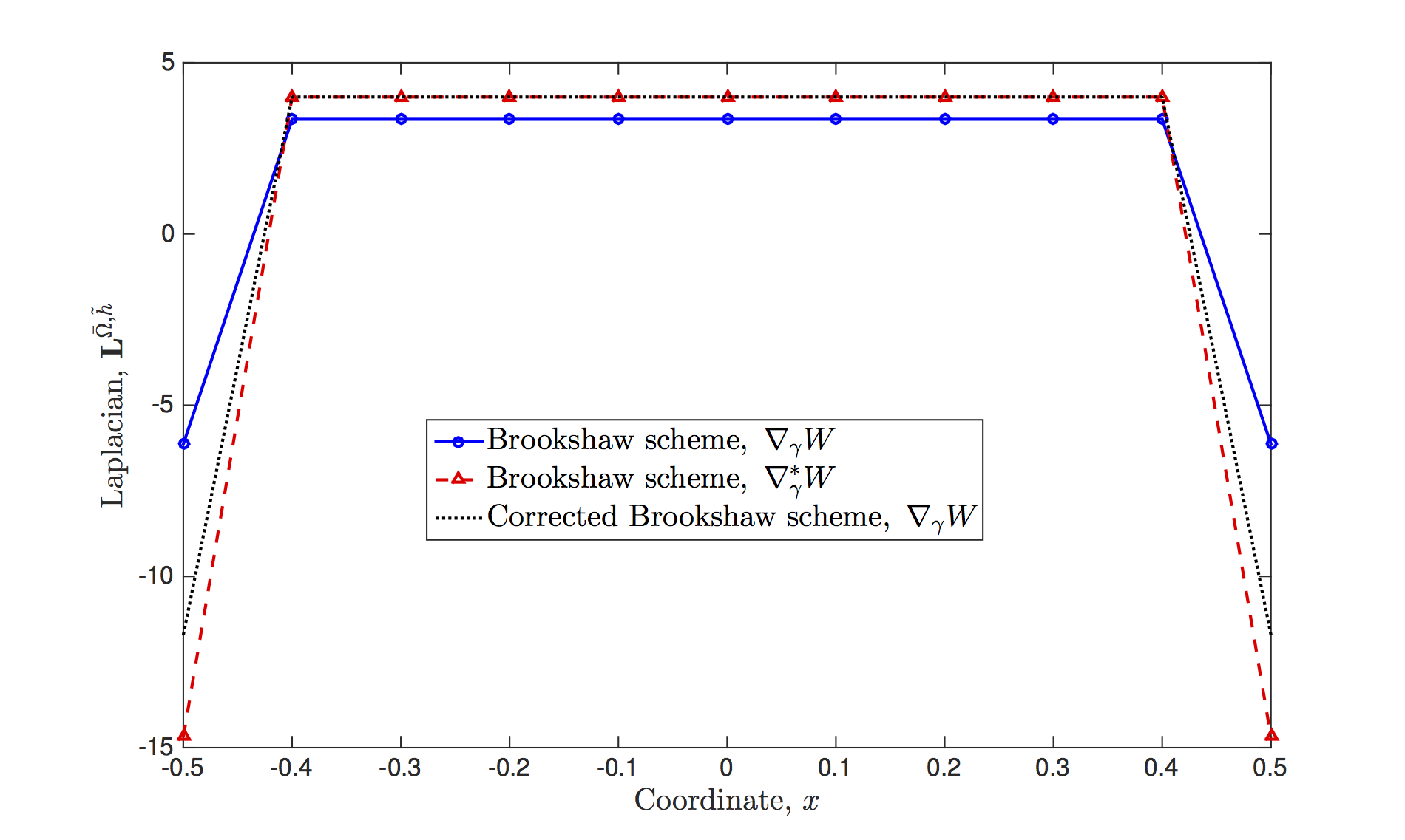
Figure 1 shows Laplacian values for the function 2(x2+y2)superscript2superscript𝑥2superscript𝑦2\nabla^{2}(x^{2}+y^{2}) using original Brookshaw’s approximation (21) with (a) conventional kernel γWsubscript𝛾𝑊\nabla_{\gamma}W, (b) corrected kernel γWsubscriptsuperscript𝛾𝑊\nabla^{*}_{\gamma}W and corrected Brookshaw’s approximation (30) with the conventional kernel γWsubscript𝛾𝑊\nabla_{\gamma}W.

Refer to caption
Figure 1. Values for 2(x2+y2)superscript2superscript𝑥2superscript𝑦2\nabla^{2}(x^{2}+y^{2}) along y=0𝑦0y=0 using Brookshaw’s approximation with (a) conventional kernel γWsubscript𝛾𝑊\nabla_{\gamma}W, (b) corrected kernel γWsubscriptsuperscript𝛾𝑊\nabla^{*}_{\gamma}W and with the correction multiplier n[𝐂αα]1𝑛superscriptdelimited-[]subscript𝐂𝛼𝛼1\displaystyle n\cdot\left[\mathbf{C}_{\alpha\alpha}\right]^{-1}. The numerical domain is a unit square in 2superscript2\mathbb{R}^{2} with the center at ai=0,isubscript𝑎𝑖0for-all𝑖a_{i}=0,\ \forall i and side length L=1𝐿1L=1. The cubic spline (9) was used with h~=fhp~𝑓subscript𝑝\tilde{h}=f\cdot h_{p}, hp=0.1subscript𝑝0.1h_{p}=0.1, f=1.0𝑓1.0f=1.0.

The scheme (21) is widely (almost unconditionally) used in the SPH modeling community. For example, it was used for a thermal conduction [1, 34, 35], for modeling a viscous diffusion [19], for a vortex spin-down [36] and Rayleigh-Taylor instability, for simulating Newtonian and non-Newtonian flows with a free surface [37] for the comparison of weakly compressible and truly incompressible algorithms, for macroscopic and mesoscopic flows [38], for a simulation of a solid-fluid mixture flow [39]. Recently, it has been used to model electrokinetic flows [40], Dam-break problem and Taylor-Green vortex [10].

There are different numerical SPH schemes used in numerical simulations. High order accuracy approximations can also be derived by using the SPH discretization on the higher order Taylor series expansion [24, 25, 2, 41]. However, it is usually required that the discrete numerical schemes can reproduce linear fields [28, 42, 13, 14] or polynomials up to a given order [43, 44].

2.4. Schwaiger’s scheme (2008)

The correction terms to the Brookshaw formulation which improve the accuracy of the Laplacian operator near boundaries were proposed by Schwaiger in [2]:

nΓkk1(m(𝒓I)𝐮(𝒓I))={Ω𝒓I,h~IV𝒓J[𝐮(𝒓J)𝐮(𝒓I)](𝒓J𝒓I)(mJ+mI)W¯(𝒓J𝒓I,h~IJ)𝒓𝒓2}{[α(m(𝒓I)𝐮(𝒓I))𝐮(𝒓I)αm(𝒓I)+m(𝒓I)α𝐮(𝒓I)]𝐍α},𝑛subscriptsuperscriptΓ1𝑘𝑘delimited-⟨⟩𝑚subscript𝒓𝐼𝐮subscript𝒓𝐼absentmissing-subexpressionmissing-subexpressionlimit-fromsubscriptsubscriptΩsubscript𝒓𝐼subscript~𝐼subscript𝑉subscript𝒓𝐽delimited-[]𝐮subscript𝒓𝐽𝐮subscript𝒓𝐼subscript𝒓𝐽subscript𝒓𝐼subscript𝑚𝐽subscript𝑚𝐼¯𝑊subscript𝒓𝐽subscript𝒓𝐼subscript~𝐼𝐽superscriptnormsuperscript𝒓𝒓2missing-subexpressionmissing-subexpressiondelimited-[]delimited-⟨⟩subscript𝛼𝑚subscript𝒓𝐼𝐮subscript𝒓𝐼𝐮subscript𝒓𝐼delimited-⟨⟩subscript𝛼𝑚subscript𝒓𝐼𝑚subscript𝒓𝐼delimited-⟨⟩subscript𝛼𝐮subscript𝒓𝐼superscript𝐍𝛼missing-subexpressionmissing-subexpression\begin{array}[]{lcl}\displaystyle\vspace{0.3cm}-\frac{n}{\Gamma^{-1}_{kk}}\langle\nabla\left(m\left(\boldsymbol{r}_{I}\right)\nabla\mathbf{u}\left(\boldsymbol{r}_{I}\right)\right)\rangle=\\ \vspace{0.3cm}\displaystyle\left\{\sum_{\Omega_{\boldsymbol{r}_{I},\tilde{h}_{I}}}V_{\boldsymbol{r}_{J}}\left[\mathbf{u}\left(\boldsymbol{r}_{J}\right)-\mathbf{u}\left(\boldsymbol{r}_{I}\right)\right]\frac{\left(\boldsymbol{r}_{J}-\boldsymbol{r}_{I}\right)\cdot\left(m_{J}+m_{I}\right)\overline{\nabla W}\left(\boldsymbol{r}_{J}-\boldsymbol{r}_{I},\tilde{h}_{IJ}\right)}{\left\|\boldsymbol{r}^{\prime}-\boldsymbol{r}\right\|^{2}}\right\}-\\ -\displaystyle\left\{\left[\langle\nabla_{\alpha}\left(m\left(\boldsymbol{r}_{I}\right)\mathbf{u}\left(\boldsymbol{r}_{I}\right)\right)\rangle-\mathbf{u}\left(\boldsymbol{r}_{I}\right)\langle\nabla_{\alpha}m\left(\boldsymbol{r}_{I}\right)\rangle+m\left(\boldsymbol{r}_{I}\right)\langle\nabla_{\alpha}\mathbf{u}\left(\boldsymbol{r}_{I}\right)\rangle\right]\mathbf{N}^{\alpha}\right\},\end{array} (31)
𝐍α(𝒓I)=[Ω𝒓I,h~IV𝒓JαW¯(𝒓I𝒓J,h~IJ)],superscript𝐍𝛼subscript𝒓𝐼delimited-[]subscriptsubscriptΩsubscript𝒓𝐼subscript~𝐼subscript𝑉subscript𝒓𝐽¯subscript𝛼𝑊subscript𝒓𝐼subscript𝒓𝐽subscript~𝐼𝐽\displaystyle\mathbf{N}^{\alpha}\left(\boldsymbol{r}_{I}\right)=\left[\sum_{\Omega_{\boldsymbol{r}_{I},\tilde{h}_{I}}}V_{\boldsymbol{r}_{J}}\overline{\nabla_{\alpha}W}\left(\boldsymbol{r}_{I}-\boldsymbol{r}_{J},\tilde{h}_{IJ}\right)\right], (32)
α𝐮(𝒓I)=Ω𝒓I,h~IV𝒓J[𝐮(𝒓J)𝐮(𝒓I)]αW¯(𝒓I𝒓J,h~IJ),delimited-⟨⟩subscript𝛼𝐮subscript𝒓𝐼subscriptsubscriptΩsubscript𝒓𝐼subscript~𝐼subscript𝑉subscript𝒓𝐽delimited-[]𝐮subscript𝒓𝐽𝐮subscript𝒓𝐼¯subscriptsuperscript𝛼𝑊subscript𝒓𝐼subscript𝒓𝐽subscript~𝐼𝐽\displaystyle\langle\nabla_{\alpha}\mathbf{u}\left(\boldsymbol{r}_{I}\right)\rangle=\sum_{\Omega_{\boldsymbol{r}_{I},\tilde{h}_{I}}}V_{\boldsymbol{r}_{J}}\left[\mathbf{u}\left(\boldsymbol{r}_{J}\right)-\mathbf{u}\left(\boldsymbol{r}_{I}\right)\right]\overline{\nabla^{*}_{\alpha}W}\left(\boldsymbol{r}_{I}-\boldsymbol{r}_{J},\tilde{h}_{IJ}\right), (33)

where n=1,2,3𝑛123n=1,2,3 is the spatial dimension and the tensor ΓαβsubscriptΓ𝛼𝛽\Gamma_{\alpha\beta} is defined by

Γαβ(𝐫I)=Ω𝒓I,h~IV𝒓J(𝒓Jγ𝒓Iγ)γW¯(𝒓J𝒓I,h~IJ)𝒓𝒓2(𝒓Jα𝒓Iα)(𝒓Jβ𝒓Iβ).subscriptΓ𝛼𝛽subscript𝐫𝐼subscriptsubscriptΩsubscript𝒓𝐼subscript~𝐼subscript𝑉subscript𝒓𝐽subscriptsuperscript𝒓𝛾𝐽subscriptsuperscript𝒓𝛾𝐼¯subscript𝛾𝑊subscript𝒓𝐽subscript𝒓𝐼subscript~𝐼𝐽superscriptnormsuperscript𝒓𝒓2subscriptsuperscript𝒓𝛼𝐽subscriptsuperscript𝒓𝛼𝐼subscriptsuperscript𝒓𝛽𝐽subscriptsuperscript𝒓𝛽𝐼\displaystyle\Gamma_{\alpha\beta}\left(\mathbf{r}_{I}\right)=\displaystyle\sum_{\Omega_{\boldsymbol{r}_{I},\tilde{h}_{I}}}V_{\boldsymbol{r}_{J}}\frac{\left(\boldsymbol{r}^{\gamma}_{J}-\boldsymbol{r}^{\gamma}_{I}\right)\overline{\nabla_{\gamma}W}\left(\boldsymbol{r}_{J}-\boldsymbol{r}_{I},\tilde{h}_{IJ}\right)}{\left\|\boldsymbol{r}^{\prime}-\boldsymbol{r}\right\|^{2}}\left(\boldsymbol{r}^{\alpha}_{J}-\boldsymbol{r}^{\alpha}_{I}\right)\left(\boldsymbol{r}^{\beta}_{J}-\boldsymbol{r}^{\beta}_{I}\right). (34)

The gradient α𝐮(𝒓I)delimited-⟨⟩subscript𝛼𝐮subscript𝒓𝐼\langle\nabla_{\alpha}\mathbf{u}\left(\boldsymbol{r}_{I}\right)\rangle is the corrected gradient which can reproduce linear fields [28, 42]. For multi-dimensional problems, the correction tensor Γαβ(𝐫I)subscriptΓ𝛼𝛽subscript𝐫𝐼\Gamma_{\alpha\beta}\left(\mathbf{r}_{I}\right) is a matrix. If the particle 𝐫Isubscript𝐫𝐼\mathbf{r}_{I} has entire stencil support (i.e., the domain support for all kernels W(𝐫J𝐫I,h~IJ)𝑊subscript𝐫𝐽subscript𝐫𝐼subscript~𝐼𝐽W\left(\mathbf{r}_{J}-\mathbf{r}_{I},\tilde{h}_{IJ}\right) is entire and symmetric) then Γαβ(𝐫I)δαβsubscriptΓ𝛼𝛽subscript𝐫𝐼subscript𝛿𝛼𝛽\Gamma_{\alpha\beta}\left(\mathbf{r}_{I}\right)\approx\delta_{\alpha\beta}.

Remark 1.

It is important to note that correction tensors ΓαβsubscriptΓ𝛼𝛽\Gamma_{\alpha\beta} and 𝐂αβ1subscriptsuperscript𝐂1𝛼𝛽\mathbf{C}^{-1}_{\alpha\beta} are the same tensors. Indeed, using the following identity:

[𝐫Jα𝐫Iα](𝐫Jγ𝐫Iγ)γW¯(𝒓J𝒓I,h~IJ)𝒓J𝒓I2==1hdW¯dz[𝒓Jα𝒓Iα]𝒓J𝒓I=αW¯(𝒓J𝒓I,h~IJ),α;dW¯dz0,delimited-[]subscriptsuperscript𝐫𝛼𝐽subscriptsuperscript𝐫𝛼𝐼subscriptsuperscript𝐫𝛾𝐽subscriptsuperscript𝐫𝛾𝐼¯subscript𝛾𝑊subscript𝒓𝐽subscript𝒓𝐼subscript~𝐼𝐽superscriptnormsubscript𝒓𝐽subscript𝒓𝐼2absentmissing-subexpressionmissing-subexpressionformulae-sequenceabsent1¯𝑑𝑊𝑑𝑧delimited-[]subscriptsuperscript𝒓𝛼𝐽subscriptsuperscript𝒓𝛼𝐼normsubscript𝒓𝐽subscript𝒓𝐼¯subscript𝛼𝑊subscript𝒓𝐽subscript𝒓𝐼subscript~𝐼𝐽for-all𝛼¯𝑑𝑊𝑑𝑧0missing-subexpressionmissing-subexpression\begin{array}[]{lcl}\displaystyle\vspace{0.3cm}\left[\mathbf{r}^{\alpha}_{J}-\mathbf{r}^{\alpha}_{I}\right]\frac{\left(\mathbf{r}^{\gamma}_{J}-\mathbf{r}^{\gamma}_{I}\right)\overline{\nabla_{\gamma}W}\left(\boldsymbol{r}_{J}-\boldsymbol{r}_{I},\tilde{h}_{IJ}\right)}{\left\|\boldsymbol{r}_{J}-\boldsymbol{r}_{I}\right\|^{2}}=\\ \displaystyle=\frac{1}{h}\frac{\overline{dW}}{dz}\frac{\left[\boldsymbol{r}^{\alpha}_{J}-\boldsymbol{r}^{\alpha}_{I}\right]}{\left\|\boldsymbol{r}_{J}-\boldsymbol{r}_{I}\right\|}=\overline{\nabla_{\alpha}W}\left(\boldsymbol{r}_{J}-\boldsymbol{r}_{I},\tilde{h}_{IJ}\right),\ \ \forall\alpha;\ \frac{\overline{dW}}{dz}\leq 0,\end{array} (35)

where dW¯dz¯𝑑𝑊𝑑𝑧\displaystyle\frac{\overline{dW}}{dz} is computed using either conventional W𝑊W or normalized W¯¯𝑊\overline{W} kernels, z=𝐫J𝐫I/h~𝑧normsubscript𝐫𝐽subscript𝐫𝐼~\displaystyle z=\left\|\boldsymbol{r}_{J}-\boldsymbol{r}_{I}\right\|/\tilde{h}, 𝐫J,𝐫IΩnfor-allsubscript𝐫𝐽subscript𝐫𝐼Ωsuperscript𝑛\forall\boldsymbol{r}_{J},\boldsymbol{r}_{I}\in\Omega\subset\mathbb{R}^{n}, the following relation can be established:

Γαβ(𝒓I)=Ω𝒓I,h~IV𝒓J(𝒓Jγ𝒓Iγ)γW¯(𝒓J𝒓I,h~IJ)𝒓J𝒓I2(𝒓Jα𝒓Iα)(𝒓Jβ𝒓Iβ)==Ω𝒓I,h~IV𝒓J[𝒓Jα𝒓Iα]βW¯(𝒓J𝒓I,h~IJ)=𝐂αβ1(𝒓I).subscriptΓ𝛼𝛽subscript𝒓𝐼subscriptsubscriptΩsubscript𝒓𝐼subscript~𝐼subscript𝑉subscript𝒓𝐽subscriptsuperscript𝒓𝛾𝐽subscriptsuperscript𝒓𝛾𝐼¯subscript𝛾𝑊subscript𝒓𝐽subscript𝒓𝐼subscript~𝐼𝐽superscriptnormsubscript𝒓𝐽subscript𝒓𝐼2subscriptsuperscript𝒓𝛼𝐽subscriptsuperscript𝒓𝛼𝐼subscriptsuperscript𝒓𝛽𝐽subscriptsuperscript𝒓𝛽𝐼absentmissing-subexpressionmissing-subexpressionabsentsubscriptsubscriptΩsubscript𝒓𝐼subscript~𝐼subscript𝑉subscript𝒓𝐽delimited-[]subscriptsuperscript𝒓𝛼𝐽subscriptsuperscript𝒓𝛼𝐼¯subscript𝛽𝑊subscript𝒓𝐽subscript𝒓𝐼subscript~𝐼𝐽subscriptsuperscript𝐂1𝛼𝛽subscript𝒓𝐼missing-subexpressionmissing-subexpression\begin{array}[]{lcl}\displaystyle\vspace{0.3cm}\Gamma_{\alpha\beta}\left(\boldsymbol{r}_{I}\right)=\sum\limits_{\Omega_{\boldsymbol{r}_{I},\tilde{h}_{I}}}V_{\boldsymbol{r}_{J}}\frac{\left(\boldsymbol{r}^{\gamma}_{J}-\boldsymbol{r}^{\gamma}_{I}\right)\overline{\nabla_{\gamma}W}\left(\boldsymbol{r}_{J}-\boldsymbol{r}_{I},\tilde{h}_{IJ}\right)}{\left\|\boldsymbol{r}_{J}-\boldsymbol{r}_{I}\right\|^{2}}\left(\boldsymbol{r}^{\alpha}_{J}-\boldsymbol{r}^{\alpha}_{I}\right)\left(\boldsymbol{r}^{\beta}_{J}-\boldsymbol{r}^{\beta}_{I}\right)=\\ \displaystyle=\sum\limits_{\Omega_{\boldsymbol{r}_{I},\tilde{h}_{I}}}V_{\boldsymbol{r}_{J}}\left[\boldsymbol{r}^{\alpha}_{J}-\boldsymbol{r}^{\alpha}_{I}\right]\overline{\nabla_{\beta}W}\left(\boldsymbol{r}_{J}-\boldsymbol{r}_{I},\tilde{h}_{IJ}\right)=\mathbf{C}^{-1}_{\alpha\beta}\left(\boldsymbol{r}_{I}\right).\end{array} (36)

In addition, it is important to note that

Γαα=Ω𝒓I,h~IV𝒓J(𝒓Jγ𝒓Iγ)γW¯(𝒓J𝒓I,h~IJ)=nsubscriptΓ𝛼𝛼subscriptsubscriptΩsubscript𝒓𝐼subscript~𝐼subscript𝑉subscript𝒓𝐽subscriptsuperscript𝒓𝛾𝐽subscriptsuperscript𝒓𝛾𝐼¯subscriptsuperscript𝛾𝑊subscript𝒓𝐽subscript𝒓𝐼subscript~𝐼𝐽𝑛\displaystyle\Gamma_{\alpha\alpha}=\sum_{\Omega_{\boldsymbol{r}_{I},\tilde{h}_{I}}}V_{\boldsymbol{r}_{J}}\left(\boldsymbol{r}^{\gamma}_{J}-\boldsymbol{r}^{\gamma}_{I}\right)\cdot\overline{\nabla^{*}_{\gamma}W}\left(\boldsymbol{r}_{J}-\boldsymbol{r}_{I},\tilde{h}_{IJ}\right)=n (37)

in the case of using the corrected gradient and, hence, Γkk1n=1subscriptsuperscriptΓ1𝑘𝑘𝑛1\displaystyle\frac{\Gamma^{-1}_{kk}}{n}=1. However, γW¯¯subscriptsuperscript𝛾𝑊\overline{\nabla^{*}_{\gamma}W} does not satisfy relation (35).

For multi-dimensional problems, the correction tensor Γαβ(𝒓I)subscriptΓ𝛼𝛽subscript𝒓𝐼\Gamma_{\alpha\beta}\left(\boldsymbol{r}_{I}\right) is a matrix. If the particle 𝒓Isubscript𝒓𝐼\boldsymbol{r}_{I} has entire stencil support (i.e., the domain support for all kernels W(𝒓J𝒓I,h~IJ)𝑊subscript𝒓𝐽subscript𝒓𝐼subscript~𝐼𝐽W\left(\boldsymbol{r}_{J}-\boldsymbol{r}_{I},\tilde{h}_{IJ}\right) is entire and symmetric) then Γαβ(𝒓I)δαβsubscriptΓ𝛼𝛽subscript𝒓𝐼subscript𝛿𝛼𝛽\Gamma_{\alpha\beta}\left(\boldsymbol{r}_{I}\right)\approx\delta_{\alpha\beta}. Unfortunately, Γαβ(𝒓I)subscriptΓ𝛼𝛽subscript𝒓𝐼\Gamma_{\alpha\beta}\left(\boldsymbol{r}_{I}\right) deviates from δαβsubscript𝛿𝛼𝛽\delta_{\alpha\beta} for the provided algorithm and, hence, it is important to minimize this deviation from δαβsubscript𝛿𝛼𝛽\delta_{\alpha\beta} in the new methods.

To calculate coefficients in the scheme (31)–(34) is a trivial task. However, in general, it should be performed at each Newton-Raphson iteration in the non-linear case (i.e., m=m(𝐮(𝒓I))𝑚𝑚𝐮subscript𝒓𝐼m=m\left(\mathbf{u}\left(\boldsymbol{r}_{I}\right)\right)). It also requires additional efforts to invert the correction matrix 𝐀αβsubscript𝐀𝛼𝛽\mathbf{A}_{\alpha\beta} (inversion of n×n𝑛𝑛n\times n matrices per each particle, where n=1,2,3𝑛123n=1,2,3 is the spatial dimension) and storage cost of αW¯(𝐫J𝐫I,h)¯subscript𝛼𝑊subscript𝐫𝐽subscript𝐫𝐼\overline{\nabla_{\alpha}W}\left(\mathbf{r}_{J}-\mathbf{r}_{I},h\right), αW¯(𝐫J𝐫I,h)¯subscriptsuperscript𝛼𝑊subscript𝐫𝐽subscript𝐫𝐼\overline{\nabla^{*}_{\alpha}W}\left(\mathbf{r}_{J}-\mathbf{r}_{I},h\right), and corresponding Γαα1=𝐀αα1subscriptsuperscriptΓ1𝛼𝛼subscriptsuperscript𝐀1𝛼𝛼\Gamma^{-1}_{\alpha\alpha}=\mathbf{A}^{-1}_{\alpha\alpha} per each particle.

Furthermore, additional terms proposed by Schwaiger [2] reduce to

[m(𝒓I)𝐮(𝒓I)𝐮(𝒓I)m(𝒓I)+m(𝒓I)𝐮(𝒓I)]𝐍==2m(𝒓I)𝐮(𝒓I)𝐍+𝒪(h~I2)delimited-[]delimited-⟨⟩𝑚subscript𝒓𝐼𝐮subscript𝒓𝐼𝐮subscript𝒓𝐼delimited-⟨⟩𝑚subscript𝒓𝐼𝑚subscript𝒓𝐼delimited-⟨⟩𝐮subscript𝒓𝐼𝐍absentmissing-subexpressionmissing-subexpressionabsent2𝑚subscript𝒓𝐼𝐮subscript𝒓𝐼𝐍𝒪superscriptsubscript~𝐼2missing-subexpressionmissing-subexpression\begin{array}[]{lcl}\displaystyle\vspace{0.2cm}\left[\left\langle m\left(\boldsymbol{r}_{I}\right)\mathbf{u}\left(\boldsymbol{r}_{I}\right)\right\rangle-\mathbf{u}\left(\boldsymbol{r}_{I}\right)\left\langle m\left(\boldsymbol{r}_{I}\right)\right\rangle+m\left(\boldsymbol{r}_{I}\right)\left\langle\mathbf{u}\left(\boldsymbol{r}_{I}\right)\right\rangle\right]\mathbf{N}=\\ \displaystyle=2m\left(\boldsymbol{r}_{I}\right)\nabla\mathbf{u}\left(\boldsymbol{r}_{I}\right)\cdot\mathbf{N}+\mathcal{O}\left(\tilde{h}_{I}^{2}\right)\end{array} (38)

which is the leading term outlined in (26). However, if one uses W¯(𝒓J𝒓I,h~IJ)¯superscript𝑊subscript𝒓𝐽subscript𝒓𝐼subscript~𝐼𝐽\overline{\nabla^{*}W}(\boldsymbol{r}_{J}-\boldsymbol{r}_{I},\tilde{h}_{IJ}) in the first term of the discretization scheme (31) then the definition for 𝐍αsuperscript𝐍𝛼\mathbf{N}^{\alpha} has to be modified in accordance of (29) to maintain the higher order discretization accuracy, for example, as:

𝐍~α=Ω𝒓I,h~IV𝒓J[𝒓Jα𝒓Iα](𝒓J𝒓I)W¯(𝒓J𝒓I,h~IJ)𝒓J𝒓I2,αsuperscript~𝐍𝛼subscriptsubscriptΩsubscript𝒓𝐼subscript~𝐼subscript𝑉subscript𝒓𝐽delimited-[]subscriptsuperscript𝒓𝛼𝐽subscriptsuperscript𝒓𝛼𝐼subscript𝒓𝐽subscript𝒓𝐼¯superscript𝑊subscript𝒓𝐽subscript𝒓𝐼subscript~𝐼𝐽superscriptnormsubscript𝒓𝐽subscript𝒓𝐼2for-all𝛼\displaystyle\widetilde{\mathbf{N}}^{\alpha}=\sum\limits_{\Omega_{\boldsymbol{r}_{I},\tilde{h}_{I}}}V_{\boldsymbol{r}_{J}}\left[\boldsymbol{r}^{\alpha}_{J}-\boldsymbol{r}^{\alpha}_{I}\right]\frac{\left(\boldsymbol{r}_{J}-\boldsymbol{r}_{I}\right)\overline{\nabla^{*}W}\left(\boldsymbol{r}_{J}-\boldsymbol{r}_{I},\tilde{h}_{IJ}\right)}{\left\|\boldsymbol{r}_{J}-\boldsymbol{r}_{I}\right\|^{2}},\ \ \ \ \forall\alpha (39)

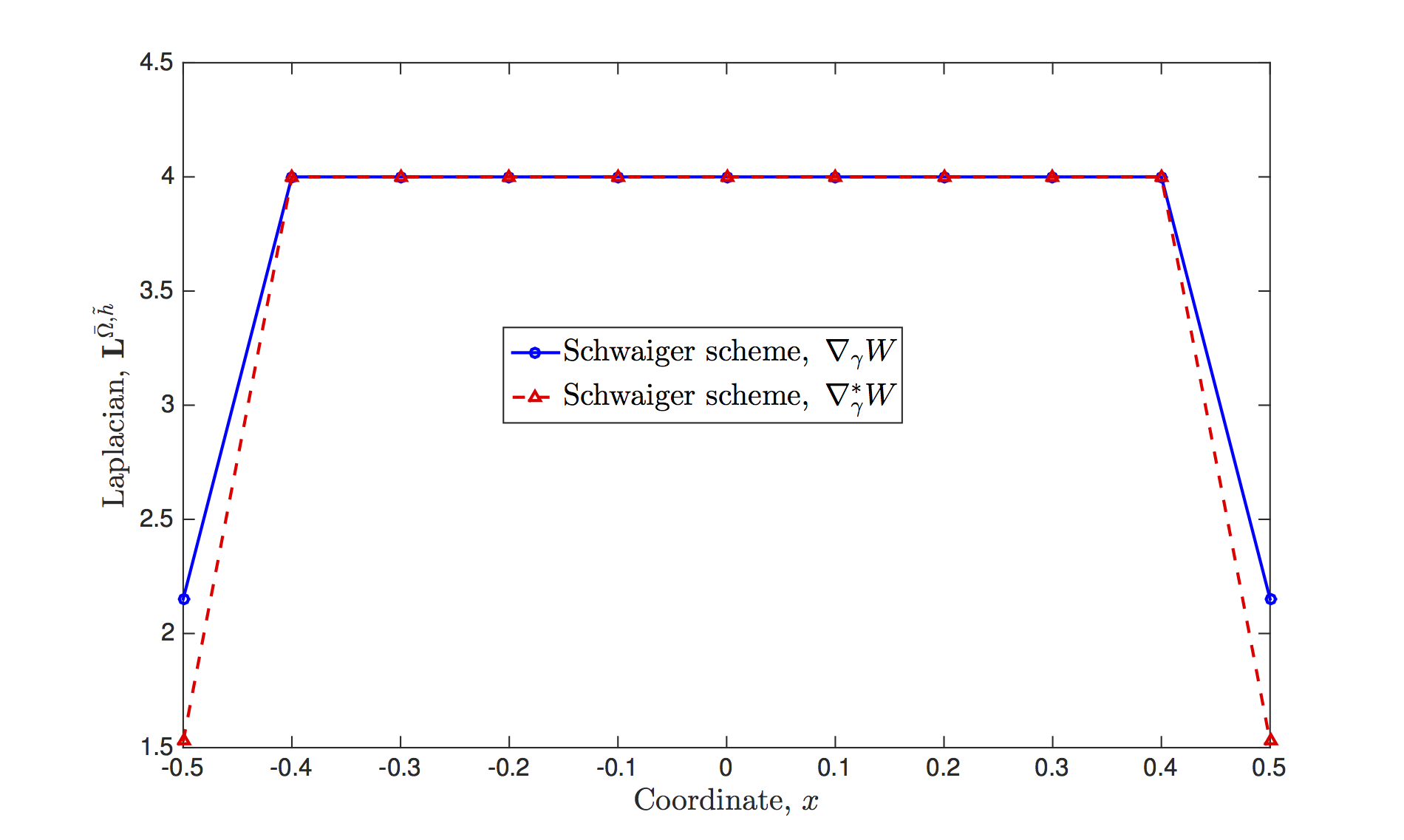
which reduces to the conventional 𝐍αsuperscript𝐍𝛼\mathbf{N}^{\alpha} in the case of W¯(𝒓J𝒓I,h~IJ)¯𝑊subscript𝒓𝐽subscript𝒓𝐼subscript~𝐼𝐽\overline{\nabla W}(\boldsymbol{r}_{J}-\boldsymbol{r}_{I},\tilde{h}_{IJ}) due to (35). Figure 2 shows the Laplacian for the function 2(x2+y2)superscript2superscript𝑥2superscript𝑦2\nabla^{2}(x^{2}+y^{2}) using Schwaiger’s approximation (31)–(34) with (a) conventional kernel γWsubscript𝛾𝑊\nabla_{\gamma}W and (b) corrected kernel γWsubscriptsuperscript𝛾𝑊\nabla^{*}_{\gamma}W.

Refer to caption
Figure 2. Values for 2(x2+y2)superscript2superscript𝑥2superscript𝑦2\nabla^{2}(x^{2}+y^{2}) along y=0𝑦0y=0 using Schwaiger’s approximation with (a) conventional kernel γWsubscript𝛾𝑊\nabla_{\gamma}W and (b) corrected kernel γWsubscriptsuperscript𝛾𝑊\nabla^{*}_{\gamma}W. The numerical domain is a unit square in in 2superscript2\mathbb{R}^{2} with the center at ai=0,isubscript𝑎𝑖0for-all𝑖a_{i}=0,\ \forall i. The cubic spline (9) was used with h~=fhp~𝑓subscript𝑝\tilde{h}=f\cdot h_{p}, hp=0.1subscript𝑝0.1h_{p}=0.1, f=1.0𝑓1.0f=1.0.

Finally, the discretization scheme (31)–(34) is at least 𝒪(hω), 1ω2𝒪superscript𝜔1𝜔2\mathcal{O}\left(h^{\omega}\right),\ 1\leq\omega\leq 2 order of accuracy in average for any scalar mobility field m(𝒓)C1(Ω),m(𝒓)0formulae-sequence𝑚𝒓superscript𝐶1Ω𝑚𝒓0m\left(\boldsymbol{r}\right)\in C^{1}\left(\Omega\right),\ m\left(\boldsymbol{r}\right)\geq 0 everywhere within the numerical domain ΩnΩsuperscript𝑛\Omega\in\mathbb{R}^{n} sufficiently far away from the boundary ΩΩ\partial\Omega.

3. Meshless Transmissibilities

The well-known two-point flux approximation (TPFA) is a mesh dependent numerical scheme used in solving elliptic equation (1): 𝐋(𝐮)=0𝐋𝐮0\mathbf{L}\left(\mathbf{u}\right)=0 with the diagonal matrix of coefficients 𝐌𝐌\mathbf{M}. The net flow rate from a cell I𝐼I into neighboring cells in this scheme is obtained by summing fluxes over the neighboring cells J𝐽J:

𝒒=JT~JI[𝐮(𝒓J)𝐮(𝒓I)],T~JI0,formulae-sequence𝒒subscript𝐽subscript~𝑇𝐽𝐼delimited-[]𝐮subscript𝒓𝐽𝐮subscript𝒓𝐼subscript~𝑇𝐽𝐼0\displaystyle\boldsymbol{q}=\sum\limits_{J}\widetilde{T}_{JI}\left[\mathbf{u}\left(\boldsymbol{r}_{J}\right)-\mathbf{u}\left(\boldsymbol{r}_{I}\right)\right],\ \widetilde{T}_{JI}\geq 0, (40)

where T~JIsubscript~𝑇𝐽𝐼\widetilde{T}_{JI} is the transmissibility between cells J𝐽J and I𝐼I, 𝒒𝒒\boldsymbol{q} is the total flux through the boundary of the control volume located at the point 𝒓Isubscript𝒓𝐼\boldsymbol{r}_{I}. The transmissibility T~JIsubscript~𝑇𝐽𝐼\widetilde{T}_{JI} defined at an interior face f𝑓f between cells J𝐽J and I𝐼I is calculated as

T~JI=1[𝒓f,J2𝑺f𝐌𝒓f,J+𝒓f,I2𝑺f𝐌𝒓f,I],subscript~𝑇𝐽𝐼1delimited-[]superscriptnormsubscript𝒓𝑓𝐽2subscript𝑺𝑓𝐌subscript𝒓𝑓𝐽superscriptnormsubscript𝒓𝑓𝐼2subscript𝑺𝑓𝐌subscript𝒓𝑓𝐼\displaystyle\widetilde{T}_{JI}=\frac{1}{\left[\displaystyle\frac{\left\|\boldsymbol{r}_{f,J}\right\|^{2}}{\boldsymbol{S}_{f}\mathbf{M}\boldsymbol{r}_{f,J}}+\frac{\left\|\boldsymbol{r}_{f,I}\right\|^{2}}{\boldsymbol{S}_{f}\mathbf{M}\boldsymbol{r}_{f,I}}\right]}, (41)

where 𝒓f,Jsubscript𝒓𝑓𝐽\boldsymbol{r}_{f,J} and 𝒓f,Isubscript𝒓𝑓𝐼\boldsymbol{r}_{f,I} are the vectors from centers of cells J𝐽J and I𝐼I to the face f𝑓f respectively, 𝑺fsubscript𝑺𝑓\boldsymbol{S}_{f} is the area vector of the face f𝑓f. In the case of 𝐌𝐌\mathbf{M}-orthogonal mesh, when 𝐌𝑺f𝐌subscript𝑺𝑓\mathbf{M}\boldsymbol{S}_{f} and [𝒓J𝒓I]delimited-[]subscript𝒓𝐽subscript𝒓𝐼\left[\boldsymbol{r}_{J}-\boldsymbol{r}_{I}\right] are collinear, the expression (40) reduces to the form of the central finite difference scheme and approximates the flux with 𝒪(h2)𝒪superscript2\mathcal{O}\left(h^{2}\right) order of accuracy for any mobility tensor field 𝐌𝐌\mathbf{M}. The expression (41) ensures that the flux into the adjoining region is continuous [34]. The TPFA scheme (40) is the unconditionally monotone scheme.

It is clear that the expression (31) cannot be written in the form (40) due to terms α(m(𝒓I)𝐮(𝒓I))𝐍αdelimited-⟨⟩subscript𝛼𝑚subscript𝒓𝐼𝐮subscript𝒓𝐼superscript𝐍𝛼\displaystyle\langle\nabla_{\alpha}\left(m\left(\boldsymbol{r}_{I}\right)\mathbf{u}\left(\boldsymbol{r}_{I}\right)\right)\rangle\mathbf{N}^{\alpha} and 𝐮(𝒓I)αm(𝒓I)𝐍α𝐮subscript𝒓𝐼delimited-⟨⟩subscript𝛼𝑚subscript𝒓𝐼superscript𝐍𝛼\displaystyle\mathbf{u}\left(\boldsymbol{r}_{I}\right)\langle\nabla_{\alpha}m\left(\boldsymbol{r}_{I}\right)\rangle\mathbf{N}^{\alpha}. Hence, it is only possible in this case to introduce a definition of a partial meshless transmissibility between particles 𝒓Jsubscript𝒓𝐽\displaystyle\boldsymbol{r}_{J} and 𝒓Isubscript𝒓𝐼\displaystyle\boldsymbol{r}_{I} as follows:

TP(𝒓J,𝒓I)=TJIP=Γββ1n×V𝒓J{(𝒓J𝒓I)(mJ+mI)W¯(𝒓J𝒓I,h~IJ)𝒓J𝒓I2mIW¯(𝒓J𝒓I,h~IJ)𝐍α}.superscript𝑇𝑃subscript𝒓𝐽subscript𝒓𝐼subscriptsuperscript𝑇𝑃𝐽𝐼subscriptsuperscriptΓ1𝛽𝛽𝑛subscript𝑉subscript𝒓𝐽missing-subexpressionmissing-subexpressionsubscript𝒓𝐽subscript𝒓𝐼subscript𝑚𝐽subscript𝑚𝐼¯𝑊subscript𝒓𝐽subscript𝒓𝐼subscript~𝐼𝐽superscriptnormsubscript𝒓𝐽subscript𝒓𝐼2subscript𝑚𝐼¯𝑊subscript𝒓𝐽subscript𝒓𝐼subscript~𝐼𝐽superscript𝐍𝛼missing-subexpressionmissing-subexpression\begin{array}[]{lcl}\vspace{0.3cm}\displaystyle T^{P}\left(\boldsymbol{r}_{J},\boldsymbol{r}_{I}\right)=T^{P}_{JI}=\frac{\Gamma^{-1}_{\beta\beta}}{n}\times V_{\boldsymbol{r}_{J}}\\ \displaystyle\left\{\frac{\left(\boldsymbol{r}_{J}-\boldsymbol{r}_{I}\right)\cdot\left(m_{J}+m_{I}\right)\cdot\overline{\nabla W}\left(\boldsymbol{r}_{J}-\boldsymbol{r}_{I},\tilde{h}_{IJ}\right)}{\left\|\boldsymbol{r}_{J}-\boldsymbol{r}_{I}\right\|^{2}}-m_{I}\overline{\nabla W}\left(\boldsymbol{r}_{J}-\boldsymbol{r}_{I},\tilde{h}_{IJ}\right)\mathbf{N}^{\alpha}\right\}.\end{array} (42)

It is important to note that transmissibilities TJIPsubscriptsuperscript𝑇𝑃𝐽𝐼T^{P}_{JI} and T~JIPsubscriptsuperscript~𝑇𝑃𝐽𝐼\widetilde{T}^{P}_{JI} have different physical units. Furthermore, it raises the question wherever the scheme (31)–(34) is monotone.

Using Taylor series expansions about a point 𝒓Isubscript𝒓𝐼\boldsymbol{r}_{I}, i.e. relations (24), (25), the expression (38) can be written keeing higher order error terms as:

[α(m(𝒓I)𝐮(𝒓I))𝐮(𝒓I)αm(𝒓I)+m(𝒓I)α𝐮(𝒓I)]=2m(𝒓I)(𝐮,α(𝒓I)+12𝐮,ωγ(𝒓I)Ω𝒓I,h~IV𝒓J[𝒓Jω𝒓Iω][𝒓Jγ𝒓Iγ]αW¯(𝒓J𝒓I,h~IJ))++𝒪(h~I3).\begin{array}[]{lcl}\displaystyle\vspace{0.3cm}\left[\left\langle\nabla_{\alpha}\left(m\left(\boldsymbol{r}_{I}\right)\mathbf{u}\left(\boldsymbol{r}_{I}\right)\right)\right\rangle-\mathbf{u}\left(\boldsymbol{r}_{I}\right)\left\langle\nabla_{\alpha}m\left(\boldsymbol{r}_{I}\right)\right\rangle+m\left(\boldsymbol{r}_{I}\right)\left\langle\nabla_{\alpha}\mathbf{u}\left(\boldsymbol{r}_{I}\right)\right\rangle\right]=\\ \vspace{0.3cm}\displaystyle 2m\left(\boldsymbol{r}_{I}\right)\left(\mathbf{u}_{,\alpha}\left(\boldsymbol{r}_{I}\right)+\frac{1}{2}\mathbf{u}_{,\omega\gamma}\left(\boldsymbol{r}_{I}\right)\sum\limits_{\Omega_{\boldsymbol{r}_{I},\tilde{h}_{I}}}V_{\boldsymbol{r}_{J}}\left[\boldsymbol{r}^{\omega}_{J}-\boldsymbol{r}^{\omega}_{I}\right]\left[\boldsymbol{r}^{\gamma}_{J}-\boldsymbol{r}^{\gamma}_{I}\right]\overline{\nabla^{*}_{\alpha}W}\left(\boldsymbol{r}_{J}-\boldsymbol{r}_{I},\tilde{h}_{IJ}\right)\right)+\\ +\mathcal{O}\left(\tilde{h}_{I}^{3}\right).\end{array} (43)

Hence, there is an additional term that has not been taken into account in (31)–(34). The following section describes an alternative numerical scheme for the heterogeneous Laplace operator. Some initial attemps were also made in [45].

3.1. New scheme

The correction terms to the Brookshaw [1] and Schwaiger [2] formulations which improve the accuracy of the Laplacian operator near boundaries can be done as follows:

nΓ¯ββ1(𝐌(𝒓I)𝐮(𝒓I))={Ω𝒓I,h~IV𝒓J[𝐮(𝒓J)𝐮(𝒓I)](𝒓J𝒓I)(𝐌J+𝐌I)W¯(𝒓J𝒓I,h~IJ)𝒓J𝒓I2}{𝐍(Ω𝒓I,h~IV𝒓J(𝐌J+𝐌I)[𝐮(𝒓J)𝐮(𝒓I)]W¯(𝒓J𝒓I,h~IJ))},𝑛subscriptsuperscript¯Γ1𝛽𝛽delimited-⟨⟩𝐌subscript𝒓𝐼𝐮subscript𝒓𝐼absentmissing-subexpressionmissing-subexpressionlimit-fromsubscriptsubscriptΩsubscript𝒓𝐼subscript~𝐼subscript𝑉subscript𝒓𝐽delimited-[]𝐮subscript𝒓𝐽𝐮subscript𝒓𝐼subscript𝒓𝐽subscript𝒓𝐼subscript𝐌𝐽subscript𝐌𝐼¯𝑊subscript𝒓𝐽subscript𝒓𝐼subscript~𝐼𝐽superscriptnormsubscript𝒓𝐽subscript𝒓𝐼2missing-subexpressionmissing-subexpression𝐍subscriptsubscriptΩsubscript𝒓𝐼subscript~𝐼subscript𝑉subscript𝒓𝐽subscript𝐌𝐽subscript𝐌𝐼delimited-[]𝐮subscript𝒓𝐽𝐮subscript𝒓𝐼¯superscript𝑊subscript𝒓𝐽subscript𝒓𝐼subscript~𝐼𝐽missing-subexpressionmissing-subexpression\begin{array}[]{lcl}\displaystyle\vspace{0.3cm}-\frac{n}{\bar{\Gamma}^{-1}_{\beta\beta}}\langle\nabla\left(\mathbf{M}\left(\boldsymbol{r}_{I}\right)\nabla\mathbf{u}\left(\boldsymbol{r}_{I}\right)\right)\rangle=\\ \vspace{0.3cm}\displaystyle\left\{\sum_{\Omega_{\boldsymbol{r}_{I},\tilde{h}_{I}}}V_{\boldsymbol{r}_{J}}\left[\mathbf{u}\left(\boldsymbol{r}_{J}\right)-\mathbf{u}\left(\boldsymbol{r}_{I}\right)\right]\frac{\left(\boldsymbol{r}_{J}-\boldsymbol{r}_{I}\right)\cdot\left(\mathbf{M}_{J}+\mathbf{M}_{I}\right)\cdot\overline{\nabla W}\left(\boldsymbol{r}_{J}-\boldsymbol{r}_{I},\tilde{h}_{IJ}\right)}{\left\|\boldsymbol{r}_{J}-\boldsymbol{r}_{I}\right\|^{2}}\right\}-\\ -\displaystyle\left\{\mathbf{N}\cdot\left(\sum\limits_{\Omega_{\boldsymbol{r}_{I},\tilde{h}_{I}}}V_{\boldsymbol{r}_{J}}\cdot(\mathbf{M}_{J}+\mathbf{M}_{I})\cdot\left[\mathbf{u}\left(\boldsymbol{r}_{J}\right)-\mathbf{u}\left(\boldsymbol{r}_{I}\right)\right]\overline{\nabla^{*}W}\left(\boldsymbol{r}_{J}-\boldsymbol{r}_{I},\tilde{h}_{IJ}\right)\right)\right\},\end{array} (44)

where n=1,2,3𝑛123n=1,2,3 is the spatial dimension and tensor Γ¯αβsubscript¯Γ𝛼𝛽\bar{\Gamma}_{\alpha\beta} is defined by

Γ¯αβ(𝒓I)={Γαβ(𝒓I),Γαβ(𝒓I)0,Γαβ(𝒓I),Γαβ(𝒓I)=0subscript¯Γ𝛼𝛽subscript𝒓𝐼casessubscriptsuperscriptΓ𝛼𝛽subscript𝒓𝐼subscriptsuperscriptΓ𝛼𝛽subscript𝒓𝐼0missing-subexpressionmissing-subexpressionsubscriptΓ𝛼𝛽subscript𝒓𝐼subscriptsuperscriptΓ𝛼𝛽subscript𝒓𝐼0missing-subexpressionmissing-subexpression\bar{\Gamma}_{\alpha\beta}\left(\boldsymbol{r}_{I}\right)=\left\{\begin{array}[]{lcl}\displaystyle\vspace{0.3cm}\Gamma^{*}_{\alpha\beta}\left(\boldsymbol{r}_{I}\right),\ \ \ \Gamma^{*}_{\alpha\beta}\left(\boldsymbol{r}_{I}\right)\neq 0,\\ \Gamma_{\alpha\beta}\left(\boldsymbol{r}_{I}\right),\ \ \ \Gamma^{*}_{\alpha\beta}\left(\boldsymbol{r}_{I}\right)=0\end{array}\right. (45)

where

Γαβ(𝒓I)=Ω𝒓I,h~IV𝒓J[𝒓Jβ𝒓Iβ]αW¯(𝒓J𝒓I,h~IJ)𝐍γΩ𝒓I,h~IV𝒓J[𝒓Jα𝒓Iα][𝒓Jβ𝒓Iβ]γW¯(𝒓J𝒓I,h~IJ).subscriptsuperscriptΓ𝛼𝛽subscript𝒓𝐼limit-fromsubscriptsubscriptΩsubscript𝒓𝐼subscript~𝐼subscript𝑉subscript𝒓𝐽delimited-[]subscriptsuperscript𝒓𝛽𝐽subscriptsuperscript𝒓𝛽𝐼¯subscript𝛼𝑊subscript𝒓𝐽subscript𝒓𝐼subscript~𝐼𝐽missing-subexpressionmissing-subexpressionsuperscript𝐍𝛾subscriptsubscriptΩsubscript𝒓𝐼subscript~𝐼subscript𝑉subscript𝒓𝐽delimited-[]subscriptsuperscript𝒓𝛼𝐽subscriptsuperscript𝒓𝛼𝐼delimited-[]subscriptsuperscript𝒓𝛽𝐽subscriptsuperscript𝒓𝛽𝐼¯subscriptsuperscript𝛾𝑊subscript𝒓𝐽subscript𝒓𝐼subscript~𝐼𝐽missing-subexpressionmissing-subexpression\begin{array}[]{lcl}\displaystyle\vspace{0.3cm}\Gamma^{*}_{\alpha\beta}\left(\boldsymbol{r}_{I}\right)=\displaystyle\sum_{\Omega_{\boldsymbol{r}_{I},\tilde{h}_{I}}}V_{\boldsymbol{r}_{J}}\left[\boldsymbol{r}^{\beta}_{J}-\boldsymbol{r}^{\beta}_{I}\right]\overline{\nabla_{\alpha}W}\left(\boldsymbol{r}_{J}-\boldsymbol{r}_{I},\tilde{h}_{IJ}\right)-\\ \displaystyle-\mathbf{N}^{\gamma}\sum\limits_{\Omega_{\boldsymbol{r}_{I},\tilde{h}_{I}}}V_{\boldsymbol{r}_{J}}\left[\boldsymbol{r}^{\alpha}_{J}-\boldsymbol{r}^{\alpha}_{I}\right]\left[\boldsymbol{r}^{\beta}_{J}-\boldsymbol{r}^{\beta}_{I}\right]\overline{\nabla^{*}_{\gamma}W}\left(\boldsymbol{r}_{J}-\boldsymbol{r}_{I},\tilde{h}_{IJ}\right).\end{array} (46)

Following (44), we only need to compute the trace of the matrix Γαβ(𝒓I)subscriptsuperscriptΓ𝛼𝛽subscript𝒓𝐼\Gamma^{*}_{\alpha\beta}\left(\boldsymbol{r}_{I}\right). Furthermore, it is important to note the following remark.

Remark 2.

The following relations can be written:

Γββ(𝒓I)=Ω𝒓I,h~IV𝒓J𝒓J𝒓I1h~IJdW¯dz𝐍γΩ𝒓I,h~IV𝒓J𝒓J𝒓I2γW¯(𝒓J𝒓I,h~IJ),dW¯dz0.subscriptsuperscriptΓ𝛽𝛽subscript𝒓𝐼limit-fromsubscriptsubscriptΩsubscript𝒓𝐼subscript~𝐼subscript𝑉subscript𝒓𝐽normsubscript𝒓𝐽subscript𝒓𝐼1subscript~𝐼𝐽¯𝑑𝑊𝑑𝑧missing-subexpressionmissing-subexpressionsuperscript𝐍𝛾subscriptsubscriptΩsubscript𝒓𝐼subscript~𝐼subscript𝑉subscript𝒓𝐽superscriptnormsubscript𝒓𝐽subscript𝒓𝐼2¯subscriptsuperscript𝛾𝑊subscript𝒓𝐽subscript𝒓𝐼subscript~𝐼𝐽¯𝑑𝑊𝑑𝑧0missing-subexpressionmissing-subexpression\begin{array}[]{lcl}\displaystyle\vspace{0.3cm}\Gamma^{*}_{\beta\beta}\left(\boldsymbol{r}_{I}\right)=\displaystyle\sum_{\Omega_{\boldsymbol{r}_{I},\tilde{h}_{I}}}V_{\boldsymbol{r}_{J}}\left\|\boldsymbol{r}_{J}-\boldsymbol{r}_{I}\right\|\frac{1}{\tilde{h}_{IJ}}\frac{\overline{dW}}{dz}-\\ \displaystyle-\mathbf{N}^{\gamma}\sum\limits_{\Omega_{\boldsymbol{r}_{I},\tilde{h}_{I}}}V_{\boldsymbol{r}_{J}}\left\|\boldsymbol{r}_{J}-\boldsymbol{r}_{I}\right\|^{2}\overline{\nabla^{*}_{\gamma}W}\left(\boldsymbol{r}_{J}-\boldsymbol{r}_{I},\tilde{h}_{IJ}\right),\ \frac{\overline{dW}}{dz}\leq 0.\end{array} (47)
|αW¯𝐍α(𝒓I)|maxzΥ(dW¯dz)2h~CαβVΩ𝒓ξΩ𝒓I,h~IVξ𝒓ξVΩ𝒓I,h~I𝒓I,\displaystyle\left|\overline{\nabla^{*}_{\alpha}W}\mathbf{N}^{\alpha}\left(\boldsymbol{r}_{I}\right)\right|\leq\max_{z\in\Upsilon}\left(\frac{\overline{dW}}{dz}\right)^{2}\cdot\tilde{h}\cdot\left\|C_{\alpha\beta}\right\|\cdot V_{\Omega}\cdot\left\|\frac{\sum\limits_{\boldsymbol{r}_{\xi}\in\Omega_{\boldsymbol{r}_{I},\tilde{h}_{I}}}V_{\xi}\cdot\boldsymbol{r}_{\xi}}{V_{\Omega_{\boldsymbol{r}_{I},\tilde{h}_{I}}}}-\boldsymbol{r}_{I}\right\|, (48)

where z=𝐫J𝐫I/h~IJ𝑧normsubscript𝐫𝐽subscript𝐫𝐼subscript~𝐼𝐽\displaystyle z=\left\|\boldsymbol{r}_{J}-\boldsymbol{r}_{I}\right\|/\tilde{h}_{IJ}, Υ=suppdW¯dzΥsupp¯𝑑𝑊𝑑𝑧\displaystyle\Upsilon=\mbox{supp}\ \frac{\overline{dW}}{dz}, Cαβnormsubscript𝐶𝛼𝛽\left\|C_{\alpha\beta}\right\| is the matrix norm of Cαβsubscript𝐶𝛼𝛽C_{\alpha\beta}, VΩ𝐫I,h~Isubscript𝑉subscriptΩsubscript𝐫𝐼subscript~𝐼V_{\Omega_{\boldsymbol{r}_{I},\tilde{h}_{I}}} is the volume of Ω𝐫I,h~IsubscriptΩsubscript𝐫𝐼subscript~𝐼\Omega_{\boldsymbol{r}_{I},\tilde{h}_{I}}. It follows that if Vξ𝐫ξVΩ𝐫I,h~I𝐫Ih~Inormsubscript𝑉𝜉subscript𝐫𝜉subscript𝑉subscriptΩsubscript𝐫𝐼subscript~𝐼subscript𝐫𝐼subscript~𝐼\displaystyle\left\|\frac{\sum V_{\xi}\boldsymbol{r}_{\xi}}{V_{\Omega_{\boldsymbol{r}_{I},\tilde{h}_{I}}}}-\boldsymbol{r}_{I}\right\|\leq\tilde{h}_{I} then there is a parameter h~Isubscript~𝐼\tilde{h}_{I} such that Γββ(𝐫I)0subscriptsuperscriptΓ𝛽𝛽subscript𝐫𝐼0\Gamma^{*}_{\beta\beta}\left(\boldsymbol{r}_{I}\right)\leq 0.

The reason for having the correction factor in the form (45)–(46) is that Γαβ(𝒓I)=0subscriptsuperscriptΓ𝛼𝛽subscript𝒓𝐼0\Gamma^{*}_{\alpha\beta}\left(\boldsymbol{r}_{I}\right)=0 in some cases, where particles have the incomplete Kernel support (e.g., at the corners and boundaries of the numerical domain). For multi-dimensional problems, the correction tensor Γ¯αβ(𝒓I)subscript¯Γ𝛼𝛽subscript𝒓𝐼\bar{\Gamma}_{\alpha\beta}\left(\boldsymbol{r}_{I}\right) is also a matrix. If the particle 𝒓Isubscript𝒓𝐼\boldsymbol{r}_{I} has entire stencil support (i.e., the domain support for all kernels W(𝒓J𝒓I,h~IJ)𝑊subscript𝒓𝐽subscript𝒓𝐼subscript~𝐼𝐽W\left(\boldsymbol{r}_{J}-\boldsymbol{r}_{I},\tilde{h}_{IJ}\right) is completed and symmetric) then Γ¯αβ(𝒓I)δαβsubscript¯Γ𝛼𝛽subscript𝒓𝐼subscript𝛿𝛼𝛽\bar{\Gamma}_{\alpha\beta}\left(\boldsymbol{r}_{I}\right)\approx\delta_{\alpha\beta}. The proposed correction matrix deviates less from the unit matrix compare to (34). As a result, the discretization scheme (44)–(46) is at least 𝒪(hω), 1ω2𝒪superscript𝜔1𝜔2\mathcal{O}\left(h^{\omega}\right),\ 1\leq\omega\leq 2 order of accuracy in average for any scalar mobility field m(𝒓)0,m(𝒓)C1(Ω)formulae-sequence𝑚𝒓0𝑚𝒓superscript𝐶1Ωm\left(\boldsymbol{r}\right)\geq 0,m\left(\boldsymbol{r}\right)\in C^{1}\left(\Omega\right), 𝐌αβ(𝒓)=m(𝒓)δαβsuperscript𝐌𝛼𝛽𝒓𝑚𝒓subscript𝛿𝛼𝛽\mathbf{M}^{\alpha\beta}\left(\boldsymbol{r}\right)=m\left(\boldsymbol{r}\right)\delta_{\alpha\beta} everywhere within the numerical domain ΩnΩsuperscript𝑛\Omega\in\mathbb{R}^{n} sufficiently far away from the boundary ΩΩ\partial\Omega. The scheme has the two-point flux approximation nature and can be written in the form of (2), which can be proved using the arguments above. The scheme (44)–(46) is in line with an alternative formulation for continuum mechanics called the peridynamic model [46, 47], which was proposed several years ago.

All presented schemes in this paper do not require exact expressions for the gradient (i.e., spatial derivatives) of the mobility field γm(𝒓)subscript𝛾𝑚𝒓\nabla_{\gamma}m\left(\boldsymbol{r}\right) to keep a higher order of accuracy for any mobility field. Hence, this scheme can be used with the discontinuous (or piecewise continuous) mobility field m(𝒓)L2(Ω)𝑚𝒓subscript𝐿2Ωm\left(\boldsymbol{r}\right)\in L_{2}\left(\Omega\right). It is important to note that Brookshaw [1] and Schwaiger [2] schemes can also be written for the diagonal mobility matrix 𝐌αβ(𝒓)superscript𝐌𝛼𝛽𝒓\mathbf{M}^{\alpha\beta}\left(\boldsymbol{r}\right) by substituting 𝐌αβsuperscript𝐌𝛼𝛽\mathbf{M}^{\alpha\beta} into (21) and (31) instead of m(𝒓)𝑚𝒓m\left(\boldsymbol{r}\right) and performing summation by repeating indices.

4. Approximation, Stability, and Monotonicity

The approximation, stability and monotonicity are important properties of numerical schemes which provide and quantify the confidence in the numerical modeling and results from corresponding simulations. Therefore, in order to be confident that the proposed numerical schemes provide the adequate accuracy of the elliptic operator (1), several numerical analyses to identify the order of approximation, stability and monotonicity have been performed. It is important to recall that all numerical schemes are characterized by two length scales: h~=fhp~𝑓subscript𝑝\tilde{h}=f\cdot h_{p} is the radius of Ω𝒓,h~=suppWsubscriptΩ𝒓~supp𝑊\Omega_{\boldsymbol{r},\tilde{h}}=\mbox{supp}W, and hpsubscript𝑝h_{p} is the inter-particle distance. Hence, while investigating the approximation of the meshless discretization scheme, it is important to distinguish two cases: (a) the neighborhood number of particles is fixed f=const𝑓constf=\mbox{const} with varying the inter-particle distance, (b) the inter-particle distance is fixed hp=constsubscript𝑝consth_{p}=\mbox{const} with varying the neighborhood number of particles. The first case will be analyzed by looking at the error defined by

EΩL2=[1JV𝒓JJV𝒓J(𝐋[𝐮(𝒓J)]𝐋[𝐮(𝒓J)])2]1/2,subscriptsuperscriptnorm𝐸subscript𝐿2Ωsuperscriptdelimited-[]1subscript𝐽subscript𝑉subscript𝒓𝐽subscript𝐽subscript𝑉subscript𝒓𝐽superscript𝐋delimited-[]𝐮subscript𝒓𝐽delimited-⟨⟩𝐋delimited-[]𝐮subscript𝒓𝐽212\left\|E\right\|^{L_{2}}_{\Omega}=\left[\frac{1}{\sum\limits_{J}V_{\boldsymbol{r}_{J}}}\sum\limits_{J}V_{\boldsymbol{r}_{J}}\left(\mathbf{L}\left[\mathbf{u}\left(\boldsymbol{r}_{J}\right)\right]-\langle\mathbf{L}\rangle\left[\mathbf{u}\left(\boldsymbol{r}_{J}\right)\right]\right)^{2}\right]^{1/2}, (49)

where 𝐋[]𝐋delimited-[]\mathbf{L}\left[\cdot\right] is the analytical Laplacian at the particle 𝒓Jsubscript𝒓𝐽\boldsymbol{r}_{J} and 𝐋[]delimited-⟨⟩𝐋delimited-[]\langle\mathbf{L}\rangle\left[\cdot\right] is the approximation of the Laplacian at the particle 𝒓Jsubscript𝒓𝐽\boldsymbol{r}_{J}, EΩL2subscriptsuperscriptnorm𝐸subscript𝐿2Ω\left\|E\right\|^{L_{2}}_{\Omega} is the averaged error over the entire domain. In the following paragraph, the numerical analysis is performed for various functions, particle distributions, and media properties.

Following the work [2], the ability of the discretization to reproduce the Laplacian was tested for several functions in n,n=1,2,3formulae-sequencesuperscript𝑛𝑛123\mathbb{R}^{n},\ n=1,2,3:

(a)𝒖s(𝒙)=i=1nxis,(b)𝒖ms(𝒙)=i=1nximi,|m|=sformulae-sequence𝑎superscript𝒖𝑠𝒙subscriptsuperscript𝑛𝑖1subscriptsuperscript𝑥𝑠𝑖formulae-sequence𝑏subscriptsuperscript𝒖𝑠𝑚𝒙subscriptsuperscriptproduct𝑛𝑖1subscriptsuperscript𝑥subscript𝑚𝑖𝑖𝑚𝑠\displaystyle\vspace{0.2cm}(a)\ \boldsymbol{u}^{s}\left(\boldsymbol{x}\right)=\sum\limits^{n}_{i=1}x^{s}_{i},\ \ \ \displaystyle(b)\ \boldsymbol{u}^{s}_{m}\left(\boldsymbol{x}\right)=\prod\limits^{n}_{i=1}x^{m_{i}}_{i},\ \left|m\right|=s (50)

where m=(m1,,mn),i:mi0:𝑚subscript𝑚1subscript𝑚𝑛for-all𝑖subscript𝑚𝑖0\displaystyle m=\left(m_{1},\ldots,m_{n}\right),\ \forall i\ :m_{i}\geq 0 is the n𝑛n-dimensional multi-index with the property |m|=i=1nmi𝑚subscriptsuperscript𝑛𝑖1subscript𝑚𝑖\left|m\right|=\sum\limits^{n}_{i=1}m_{i}. The reason for selecting these testing polynomials is as follows. Since the functional space Lp(Ω)subscript𝐿𝑝ΩL_{p}\left(\Omega\right) is separable, the above polynomials form the everywhere dense subset of the Lp(Ω)subscript𝐿𝑝ΩL_{p}\left(\Omega\right). Hence, any function 𝐮Lp𝐮subscript𝐿𝑝\mathbf{u}\in L_{p} can be approximated in Lpsubscript𝐿𝑝L_{p} using linear combination of the above polynomials leading to the following relations:

𝐮(𝒓)k=1|m|kam(i=1nximi),𝐌(𝒓)k=1|m|kbm(i=1nximi).formulae-sequence𝐮𝒓subscriptsuperscript𝑘1subscript𝑚𝑘subscript𝑎𝑚subscriptsuperscriptproduct𝑛𝑖1subscriptsuperscript𝑥subscript𝑚𝑖𝑖𝐌𝒓subscriptsuperscript𝑘1subscript𝑚𝑘subscript𝑏𝑚subscriptsuperscriptproduct𝑛𝑖1subscriptsuperscript𝑥subscript𝑚𝑖𝑖\displaystyle\mathbf{u}(\boldsymbol{r})\approx\sum\limits^{\infty}_{k=1}\sum\limits_{\left|m\right|\leq k}a_{m}\left(\prod\limits^{n}_{i=1}x^{m_{i}}_{i}\right),\mathbf{M}\left(\boldsymbol{r}\right)\approx\sum\limits^{\infty}_{k=1}\sum\limits_{\left|m\right|\leq k}b_{m}\left(\prod\limits^{n}_{i=1}x^{m_{i}}_{i}\right). (51)

The approximation error produced by the discretization schemes and considered in this paper for the polynomials 𝒖s(𝒙)superscript𝒖𝑠𝒙\boldsymbol{u}^{s}\left(\boldsymbol{x}\right) and 𝒖ms(𝒙)subscriptsuperscript𝒖𝑠𝑚𝒙\boldsymbol{u}^{s}_{m}\left(\boldsymbol{x}\right) gives the information about the error growth for the arbitrary function 𝐮(𝒓)𝐮𝒓\mathbf{u}(\boldsymbol{r}). In each test, the homogenous and heterogeneous particle distribution varying the smoothing length h~~\tilde{h} and inter-particle distance hpsubscript𝑝h_{p} are used to study the approximation properties of the proposed discretization scheme.

4.1. Isotropic Homogeneous Media

Note that in the limit of the homogeneous isotropic media (i.e., 𝐌αβ(𝒓)=m(𝒓)δαβsuperscript𝐌𝛼𝛽𝒓𝑚𝒓subscript𝛿𝛼𝛽\mathbf{M}^{\alpha\beta}\left(\boldsymbol{r}\right)=m\left(\boldsymbol{r}\right)\delta_{\alpha\beta}, m(𝒓)=1𝑚𝒓1m\left(\boldsymbol{r}\right)=1) and without the source term, the aforementioned operator 𝐋(𝐮)𝐋𝐮\mathbf{L}\left(\mathbf{u}\right) in (1) reduces to the conventional Laplacian operator (i.e., 𝐋(𝐮)2𝐮𝐋𝐮superscript2𝐮\mathbf{L}\left(\mathbf{u}\right)\equiv\nabla^{2}\mathbf{u}). The domain for the patch test is a unit square similar to [2] for n=2𝑛2n=2:

Ω={𝒓={xi}n||xi2.5|12i}\displaystyle\Omega=\left\{\boldsymbol{r}=\left\{x_{i}\right\}\in\mathbb{R}^{n}\left|\right.\ \ \left|x_{i}-2.5\right|\leqslant\frac{1}{2}\ \ \forall i\right\}

with N=21𝑁21N=21 particles in each direction characterized by two length spacings: h~=fhp~𝑓subscript𝑝\tilde{h}=f\cdot h_{p}, hp=0.05subscript𝑝0.05h_{p}=0.05, f=1.2𝑓1.2f=1.2.

In all of the following tests, the results are displayed along the cross-section y=2.5𝑦2.5y=2.5 in n,n=2superscript𝑛𝑛2\mathbb{R}^{n},\ n=2 (similar to [2] for n=2𝑛2n=2). In each test, the following discretizations are compared: corrected Brookshaw’s scheme (CB-SPH) (30), Schwaiger’s scheme (S-SPH) (31)–(34), and new proposed scheme (M-SPH) (44)–(46). Note that the Schwaiger’s scheme was tested against several schemes published in [30], [23] and show better accuracy; hence, schemes in [30], [23] are not considered in this paper. The comparison of different schemes starts with test functions of the form 𝐮s(𝒙)superscript𝐮𝑠𝒙\mathbf{u}^{s}\left(\boldsymbol{x}\right) described by (50)(a) in n,n=2superscript𝑛𝑛2\mathbb{R}^{n},\ n=2. Plots of the Laplacian approximations and the relative errors defined by (49) for the case m=3𝑚3m=3 are shown in Figure 3.

Refer to caption        Refer to caption

Figure 3. Cross-section of the test patch at y=2.5𝑦2.5y=2.5. Three SPH approximations of 2(x3+y3)superscript2superscript𝑥3superscript𝑦3\nabla^{2}\left(x^{3}+y^{3}\right) with different kernel gradients are shown. Corrected Brookshaw’s scheme (CB-SPH) is given by (30) with the correction multiplier, while Schwaiger’s scheme (S-SPH) is given by (31)–(34). New approximation (M-SPH) considered here is the SPH form (44)–(46). In this case, the Schwaiger’s scheme and new scheme have comparable accuracy at the boundaries and are accurate in the interior to the machine precision. Four different options of computing the kernel gradient (i.e., γWsubscript𝛾𝑊\nabla_{\gamma}W, αW¯subscript𝛼¯𝑊\nabla_{\alpha}\overline{W}, and corrected kernel gradients (i.e., αWsubscriptsuperscript𝛼𝑊\nabla^{*}_{\alpha}W, αW¯subscriptsuperscript𝛼¯𝑊\nabla^{*}_{\alpha}\overline{W}, ¯αW¯subscriptsuperscript¯𝛼¯𝑊\overline{\nabla}^{*}_{\alpha}\overline{W}, and ~αW¯subscriptsuperscript~𝛼¯𝑊\widetilde{\nabla}^{*}_{\alpha}\overline{W}) are shown.

The new scheme (M-SPH) has the greatest accuracy at the boundary and is accurate to machine precision ε𝜀\varepsilon in the interior. The error plot is shown in Figure 4 along with test functions with exponents from m=4,,7𝑚47m=4,...,7. For these functions, the proposed scheme (44)–(46) is uniformly more accurate for the various experiments.
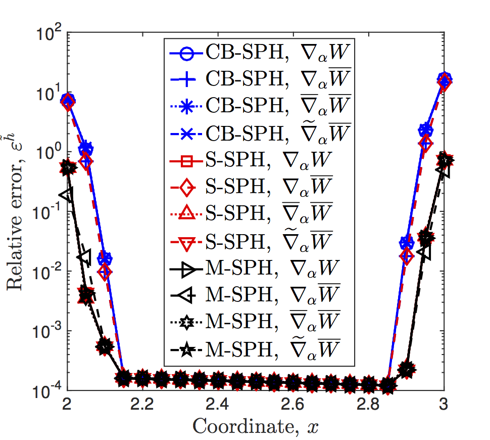
Refer to caption m=4          Refer to caption m=5
Refer to caption m=6          Refer to caption m=7

Figure 4. The relative errors along y=2.5𝑦2.5y=2.5 for each of the discretizations used in Figure 3 are shown here for the suite of functions 2(xm+ym)superscript2superscript𝑥𝑚superscript𝑦𝑚\nabla^{2}\left(x^{m}+y^{m}\right) where m=4,,7𝑚47m=4,\ldots,7. Four different options of computing the kernel gradients (i.e., γWsubscript𝛾𝑊\nabla_{\gamma}W, αW¯subscript𝛼¯𝑊\nabla_{\alpha}\overline{W}, and corrected kernel gradients (i.e., γWsubscriptsuperscript𝛾𝑊\nabla^{*}_{\gamma}W, αW¯subscriptsuperscript𝛼¯𝑊\nabla^{*}_{\alpha}\overline{W}, ¯αW¯subscriptsuperscript¯𝛼¯𝑊\overline{\nabla}^{*}_{\alpha}\overline{W}, and ~αW¯subscriptsuperscript~𝛼¯𝑊\widetilde{\nabla}^{*}_{\alpha}\overline{W}) are shown.

The same behavior is observed in 3D where the M-SPH scheme with the αW¯subscript𝛼¯𝑊\nabla_{\alpha}\overline{W} is the most accurate scheme. Furthermore, the new scheme should be tested for the functions requiring cross-derivatives as was reported in [2]. To examine the effect of the cross-derivative terms, the same suite of tests was run with the function 𝒖ms(𝒙)subscriptsuperscript𝒖𝑠𝑚𝒙\boldsymbol{u}^{s}_{m}\left(\boldsymbol{x}\right) described by (50)(b) in n,n=2,3formulae-sequencesuperscript𝑛𝑛23\mathbb{R}^{n},\ n=2,3. Relative errors for (xy)msuperscript𝑥𝑦𝑚(xy)^{m} on a same array as in Figure 3 along y=2.5𝑦2.5y=2.5 were computed and again the proposed scheme (44)–(46) was uniformly more accurate for the various experiments. The behavior of each discretization is similar to that shown in Figure 3. The proposed new scheme (M-SPH) performed nearly as well as the Schwaiger’s scheme at the boundary. The CB-SPH and S-SPH forms also perform with greater accuracy than all other forms in the interior except in the case with the highest exponent.

An additional concern is that although it deviates from the exact solution near boundaries, it acquires no off-diagonal terms due to the alignment of the array of particles and the boundaries with the coordinate axes. To test the accuracy of the new approximations when there are off-diagonal terms, an array with particles rotated 45osuperscript45𝑜45^{o} was used with the test function (xy)msuperscript𝑥𝑦𝑚(xy)^{m} (similar to [2]). The new proposed scheme formulation performs consistently well for lower exponents.

4.2. Isotropic Heterogeneous Media

In isotropic heterogeneous media, i.e., 𝐌αβ(𝒓)=m(𝒓)δαβsuperscript𝐌𝛼𝛽𝒓𝑚𝒓subscript𝛿𝛼𝛽\mathbf{M}^{\alpha\beta}\left(\boldsymbol{r}\right)=m\left(\boldsymbol{r}\right)\delta_{\alpha\beta}, the Laplace operator takes the general form written in (1). The numerical domain is the same as in the previous section with the same number of particles and particle length scales: h~=fhp~𝑓subscript𝑝\tilde{h}=f\cdot h_{p}, hp=0.05subscript𝑝0.05h_{p}=0.05, f=1.2𝑓1.2f=1.2. Plots of the Laplacian approximations and the relative errors defined by (49) for the case of heterogeneous mobility with m=1𝑚1m=1 (see (51)) are shown in Figure 5.

Refer to caption        Refer to caption

Figure 5. Cross-section of the test patch at y=2.5𝑦2.5y=2.5. Three SPH approximations of ((x+y)((x+y)))𝑥𝑦𝑥𝑦\nabla(\left(x+y\right)(\nabla\left(x+y\right))) with different kernel gradients are shown. The different schemes and kernel gradients are described in the caption of Figure (3).

The new scheme (M-SPH) has the best accuracy at the boundary and is accurate to machine precision ε𝜀\varepsilon in the interior. The error plot is shown in Figure 6 along with test functions with exponents from m=2,,5𝑚25m=2,...,5. For these functions, the proposed scheme (44)-(46) is uniformly more accurate for the different increasing exponents.
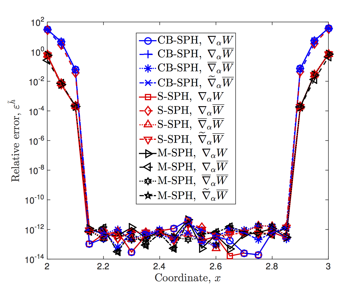
Refer to caption m=2          Refer to caption m=3
Refer to caption m=4          Refer to caption m=5

Figure 6. The relative errors along y=2.5𝑦2.5y=2.5 for each of the discretizations used in Figure 3 are shown here only for the suite of functions [(xm+ym)(x+y)]superscript𝑥𝑚superscript𝑦𝑚𝑥𝑦\displaystyle\nabla\left[\left(x^{m}+y^{m}\right)\nabla\left(x+y\right)\right] where m=2,,5𝑚25m=2,\ldots,5. Four different options of computing kernel gradients (i.e., γWsubscript𝛾𝑊\nabla_{\gamma}W, αW¯subscript𝛼¯𝑊\nabla_{\alpha}\overline{W}), and corrected kernel gradients (i.e., γWsubscriptsuperscript𝛾𝑊\nabla^{*}_{\gamma}W, αW¯subscriptsuperscript𝛼¯𝑊\nabla^{*}_{\alpha}\overline{W}, ¯αW¯subscriptsuperscript¯𝛼¯𝑊\overline{\nabla}^{*}_{\alpha}\overline{W}, and ~αW¯subscriptsuperscript~𝛼¯𝑊\widetilde{\nabla}^{*}_{\alpha}\overline{W}) are shown.

The same behavior is observed in 3D where M-SPH scheme with the αW¯subscript𝛼¯𝑊\nabla_{\alpha}\overline{W} is the most accurate scheme.

4.3. von Neumann stability analysis

For linear PDEs, there is the Lax-equivalence theorem which connects the consistency and stability with the convergence. The idea of the von Neumann stability analysis is to study the growth of waves λei𝒌𝒓𝜆superscript𝑒𝑖𝒌𝒓\lambda e^{i\boldsymbol{k}\cdot\boldsymbol{r}} (similar to Fourier methods). After applying one of the discretization methods above to the Laplace operator (1), the following relation can be written:

{𝐮}n+1{𝐮}nτ𝐋h~[{𝐮}n]={𝒃},superscript𝐮𝑛1superscript𝐮𝑛𝜏superscript𝐋~delimited-[]superscript𝐮𝑛𝒃\displaystyle\frac{\left\{\mathbf{u}\right\}^{n+1}-\left\{\mathbf{u}\right\}^{n}}{\tau}-\mathbf{L}^{\tilde{h}}\left[\left\{\mathbf{u}\right\}^{n}\right]=\left\{\boldsymbol{b}\right\}, (52)

where τ𝜏\tau is the iteration parameter (e.g., time step), n𝑛n is the iteration index (e.g., time index), {𝐮}n=(𝒖1n,,𝒖Nn)superscript𝐮𝑛subscriptsuperscript𝒖𝑛1subscriptsuperscript𝒖𝑛𝑁\left\{\mathbf{u}\right\}^{n}=\left(\boldsymbol{u}^{n}_{1},\ldots,\boldsymbol{u}^{n}_{N}\right) is a vector of all N𝑁N particle values 𝒖in,i=1,,Nformulae-sequencesubscriptsuperscript𝒖𝑛𝑖𝑖1𝑁\boldsymbol{u}^{n}_{i},\ i=1,\ldots,N, {𝒃}=(𝒃1,,𝒃N)𝒃subscript𝒃1subscript𝒃𝑁\left\{\boldsymbol{b}\right\}=\left(\boldsymbol{b}_{1},\ldots,\boldsymbol{b}_{N}\right) is the right-hand side vector. The expression (52) may represent, for example, discretization of the parabolic PDE or an iterative solver of the linear system of equations arising from discretization of elliptic boundary value problem. Substituting into the left-hand side of the relation (52) the following form of perturbation

𝒖jn=λnei𝒌j𝒓j=λnl=1neikjlxjlsubscriptsuperscript𝒖𝑛𝑗superscript𝜆𝑛superscript𝑒isubscript𝒌𝑗subscript𝒓𝑗superscript𝜆𝑛subscriptsuperscriptproduct𝑛𝑙1superscript𝑒isubscriptsuperscript𝑘𝑙𝑗subscriptsuperscript𝑥𝑙𝑗\displaystyle\boldsymbol{u}^{n}_{j}=\lambda^{n}e^{\textbf{i}\boldsymbol{k}_{j}\cdot\boldsymbol{r}_{j}}=\lambda^{n}\cdot\prod\limits^{n}_{l=1}e^{\textbf{i}k^{l}_{j}\cdot x^{l}_{j}} (53)

leads to the expression for the von Neumann growth factor subject to (52) and linear Laplace operator:

λj(τ)=1+τei𝒌j𝒓j𝐋h~[{ei𝒌𝒓}],𝒓n,n=1,2,3;formulae-sequencesubscript𝜆𝑗𝜏1𝜏superscript𝑒isubscript𝒌𝑗subscript𝒓𝑗superscript𝐋~delimited-[]superscript𝑒i𝒌𝒓formulae-sequence𝒓superscript𝑛𝑛123\displaystyle\lambda_{j}\left(\tau\right)=1+\tau\cdot e^{-\textbf{i}\boldsymbol{k}_{j}\cdot\boldsymbol{r}_{j}}\cdot{\mathbf{L}}^{\tilde{h}}\left[\left\{e^{\textbf{i}\boldsymbol{k}\cdot\boldsymbol{r}}\right\}\right],\boldsymbol{r}\in\mathbb{R}^{n},\ n=1,2,3; (54)

where {ei𝒌𝒓}=(ei𝒌1𝒓1,,ei𝒌N𝒓N)superscript𝑒i𝒌𝒓superscript𝑒isubscript𝒌1subscript𝒓1superscript𝑒isubscript𝒌𝑁subscript𝒓𝑁\left\{e^{\textbf{i}\boldsymbol{k}\cdot\boldsymbol{r}}\right\}=\left(e^{\textbf{i}\boldsymbol{k}_{1}\cdot\boldsymbol{r}_{1}},\ldots,e^{\textbf{i}\boldsymbol{k}_{N}\cdot\boldsymbol{r}_{N}}\right) and λj(τ)subscript𝜆𝑗𝜏\lambda_{j}\left(\tau\right) is the von Neumann growth factor. For the discretization to be stable, it is required that |λj(τ)|1,jsubscript𝜆𝑗𝜏1for-all𝑗\left|\lambda_{j}\left(\tau\right)\right|\leq 1,\ \forall j. The von Neumann growth factor is shown for three main discretization schemes: Corrected Brookshaw’s scheme (CB-SPH) (30), Schwaiger’s scheme (S-SPH) (31)–(34) and new approximation (M-SPH) (44)–(46) for uniform and pseudo random particle distribution with τ=0.25𝜏0.25\tau=0.25 and 𝐌αβ(𝒓)=δαβsuperscript𝐌𝛼𝛽𝒓subscript𝛿𝛼𝛽\mathbf{M}^{\alpha\beta}\left(\boldsymbol{r}\right)=\delta_{\alpha\beta} (see, Figures 7). In case of uniform particle distribution, the von Neumann growth factor clusters around the real axis for all schemes and satisfies the requirement |λj(τ)|1,jsubscript𝜆𝑗𝜏1for-all𝑗\left|\lambda_{j}\left(\tau\right)\right|\leq 1,\ \forall j. In case of pseudo random particle distribution, the von Neumann growth factor has both real and imaginary parts forming complex shape but satisfying the requirement |λj(τ)|1,jsubscript𝜆𝑗𝜏1for-all𝑗\left|\lambda_{j}\left(\tau\right)\right|\leq 1,\ \forall j almost everywhere (i.e., it could be some problems at the boundary particles).
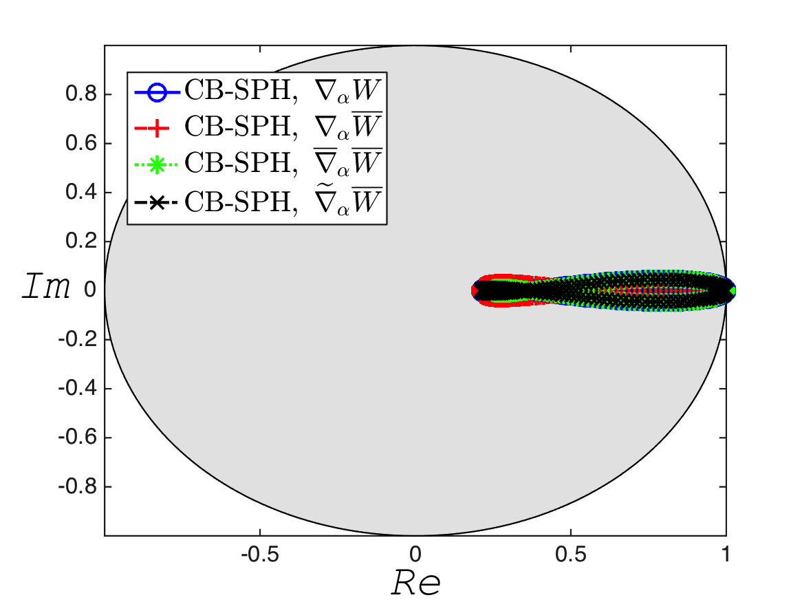
Refer to caption Uniform Refer to caption Uniform Refer to caption Uniform
Refer to caption Random Refer to caption Random Refer to caption Random

Figure 7. von Neumann growth factor for different discretization schemes. Corrected Brookshaw’s scheme (CB-SPH) is given by (30) with the correction multiplier, while Schwaiger’s scheme (S-SPH) is given by (31)–(34). New approximation (M-SPH) considered here are the SPH form (44)–(46). Four different options of computing kernel gradients (i.e., γWsubscript𝛾𝑊\nabla_{\gamma}W, αW¯subscript𝛼¯𝑊\nabla_{\alpha}\overline{W}, and corrected kernel gradients (i.e., γWsubscriptsuperscript𝛾𝑊\nabla^{*}_{\gamma}W, αW¯subscriptsuperscript𝛼¯𝑊\nabla^{*}_{\alpha}\overline{W}, ¯αW¯subscriptsuperscript¯𝛼¯𝑊\overline{\nabla}^{*}_{\alpha}\overline{W}, and ~αW¯subscriptsuperscript~𝛼¯𝑊\widetilde{\nabla}^{*}_{\alpha}\overline{W}) are shown.

4.4. Monotonicity and Convergence

In real life applications, the numerical domains are large and, therefore, many degree of freedom (i.e., unknowns) is required. The resulting matrix is usually sparse, but because of fill-in a direct method requires significant amount of memory and time in general case. Hence, iterative solvers are used to overcome these issues. The iterative solvers converge only if the matrix satisfies certain properties related to the property of the diagonal dominance. However, these properties are only sufficient conditions for the method to converge.

The proof of the convergence of linear meshless schemes applied to a linear elliptic boundary value problem can be done in the following steps (see, Bouchon (2007) [48], Bouchon and Peichl (2007) [49], Matsunaga and Yamamoto (2000) [50], Thomée (2001) [51]: if it is shown that the truncation error ε𝜀\varepsilon tends to 0 as the maximum smoothing length maxINhIsubscript𝐼𝑁subscript𝐼\max\limits_{I\in N}h_{I} goes to 0, then the linear system Aδu=εA𝛿𝑢𝜀\textbf{A}\delta u=\varepsilon that couples the variable error δu𝛿𝑢\delta u with ε𝜀\varepsilon proves the convergence of the schemes, given that the matrix of the discretized meshless operator is monotone. A square matrix 𝐀=(aij)1in,1jnn×n𝐀subscriptsubscript𝑎𝑖𝑗formulae-sequence1𝑖𝑛1𝑗𝑛superscript𝑛𝑛\mathbf{A}=\left(a_{ij}\right)_{1\leq i\leq n,1\leq j\leq n}\in\mathbb{R}^{n\times n} is called monotone if aij0ijsubscript𝑎𝑖𝑗0for-all𝑖𝑗a_{ij}\leq 0\ \forall i\neq j, aii>0isubscript𝑎𝑖𝑖0for-all𝑖a_{ii}>0\ \forall i and it is inverse positive 𝐀10superscript𝐀10\mathbf{A}^{-1}\geq 0. Furthermore, the monotone schemes do satisfy a discrete maximum principle producing solutions without spurious oscillations.

It is clear that the new scheme (44)–(46) can be written in the form (40), where meshless transmissibility between particles 𝐫Jsubscript𝐫𝐽\displaystyle\mathbf{r}_{J} and 𝐫Isubscript𝐫𝐼\displaystyle\mathbf{r}_{I} can be defined as T(𝐫J,𝐫I)=Γ¯ββn(mI+mJ)T¯IJ𝑇subscript𝐫𝐽subscript𝐫𝐼subscript¯Γ𝛽𝛽𝑛subscript𝑚𝐼subscript𝑚𝐽subscript¯𝑇𝐼𝐽\displaystyle T\left(\mathbf{r}_{J},\mathbf{r}_{I}\right)=\frac{\bar{\Gamma}_{\beta\beta}}{n}\left(m_{I}+m_{J}\right)\bar{T}_{IJ} with:

T¯IJ={(𝒓J𝒓I)W¯(𝒓J𝒓I,h~IJ)𝒓J𝒓I2αW¯(𝒓J𝒓I,h~IJ)𝐍α},subscript¯𝑇𝐼𝐽subscript𝒓𝐽subscript𝒓𝐼¯𝑊subscript𝒓𝐽subscript𝒓𝐼subscript~𝐼𝐽superscriptnormsubscript𝒓𝐽subscript𝒓𝐼2¯subscriptsuperscript𝛼𝑊subscript𝒓𝐽subscript𝒓𝐼subscript~𝐼𝐽superscript𝐍𝛼missing-subexpressionmissing-subexpression\begin{array}[]{lcl}\displaystyle\bar{T}_{IJ}=\displaystyle\left\{\frac{\left(\boldsymbol{r}_{J}-\boldsymbol{r}_{I}\right)\cdot\overline{\nabla W}\left(\boldsymbol{r}_{J}-\boldsymbol{r}_{I},\tilde{h}_{IJ}\right)}{\left\|\boldsymbol{r}_{J}-\boldsymbol{r}_{I}\right\|^{2}}-\overline{\nabla^{*}_{\alpha}W}\left(\boldsymbol{r}_{J}-\boldsymbol{r}_{I},\tilde{h}_{IJ}\right)\mathbf{N}^{\alpha}\right\},\end{array} (55)

where 𝐍α(𝒓I)superscript𝐍𝛼subscript𝒓𝐼\mathbf{N}^{\alpha}\left(\boldsymbol{r}_{I}\right) is defined by (32). This allows us to formulate the following remark.

Remark 3.

Taking into account Remark 2 and the following relation:

(𝒓J𝒓I)W¯(𝒓J𝒓I,h)𝒓J𝒓I2=1zh2dW¯dz(z)0,subscript𝒓𝐽subscript𝒓𝐼¯𝑊subscript𝒓𝐽subscript𝒓𝐼superscriptnormsubscript𝒓𝐽subscript𝒓𝐼21𝑧superscript2¯𝑑𝑊𝑑𝑧𝑧0missing-subexpressionmissing-subexpression\begin{array}[]{lcl}\displaystyle\vspace{0.3cm}\frac{\left(\boldsymbol{r}_{J}-\boldsymbol{r}_{I}\right)\cdot\overline{\nabla W}\left(\boldsymbol{r}_{J}-\boldsymbol{r}_{I},h\right)}{\left\|\boldsymbol{r}_{J}-\boldsymbol{r}_{I}\right\|^{2}}=\frac{1}{z\cdot h^{2}}\frac{\overline{dW}}{dz}\left(z\right)\leq 0,\end{array} (56)

and the relation (48) which all together lead to the fact that there is a parameter h~Isubscript~𝐼\tilde{h}_{I} such that T(𝐫J,𝐫I)0𝑇subscript𝐫𝐽subscript𝐫𝐼0T\left(\mathbf{r}_{J},\mathbf{r}_{I}\right)\geq 0. This means that the proposed scheme subject to this parameter h~Isubscript~𝐼\tilde{h}_{I} is monotone for the medium with the scalar heterogeneous coefficients.

5. Solution of Boundary Value Problems

Following the work by [2], the numerical tests for inhomogeneous Dirichlet, Neumann and mixed boundary conditions are considered for homogeneous and heterogeneous media with the characteristics 𝐌(𝒓)𝐌𝒓\mathbf{M}\left(\boldsymbol{r}\right). To illustrate the performance of the proposed scheme, a modelling of a single phase steady-state fluid flow in fully anisotropic porous media with different type of boundary conditions is also presented in this section. The square 2D and 3D domains (3) are considered.

The relative error used to quantify the accuracy of the proposed schemes in the subsections (2.3), (2.4), and (3.1) during numerical simulation in this section is given by:

ERΩL2=[1ΩV𝒓JΩV𝒓K(𝐮(𝒓K)𝐮(𝒓K)𝐮(𝒓K))2]1/2subscriptsuperscriptnormsubscript𝐸𝑅subscript𝐿2Ωsuperscriptdelimited-[]1subscriptΩsubscript𝑉subscript𝒓𝐽subscriptΩsubscript𝑉subscript𝒓𝐾superscript𝐮subscript𝒓𝐾delimited-⟨⟩𝐮subscript𝒓𝐾𝐮subscript𝒓𝐾212\displaystyle\left\|E_{R}\right\|^{L_{2}}_{\Omega}=\left[\frac{1}{\sum\limits_{\Omega}V_{\boldsymbol{r}_{J}}}\sum\limits_{\Omega}V_{\boldsymbol{r}_{K}}\left(\frac{\mathbf{u}\left(\boldsymbol{r}_{K}\right)-\langle\mathbf{u}\left(\boldsymbol{r}_{K}\right)\rangle}{\mathbf{u}\left(\boldsymbol{r}_{K}\right)}\right)^{2}\right]^{1/2} (57)

where 𝐮(𝒓)𝐮𝒓\mathbf{u}\left(\boldsymbol{r}\right) is the analytical or reference solution field and 𝐮(𝒓K)delimited-⟨⟩𝐮subscript𝒓𝐾\langle\mathbf{u}\left(\boldsymbol{r}_{K}\right)\rangle is the approximated solution field. Several numerical results using considered in this paper schemes for uniform and pseudo random particle distributions are shown in the following sections that confirm the theoretical results from the previous sections.
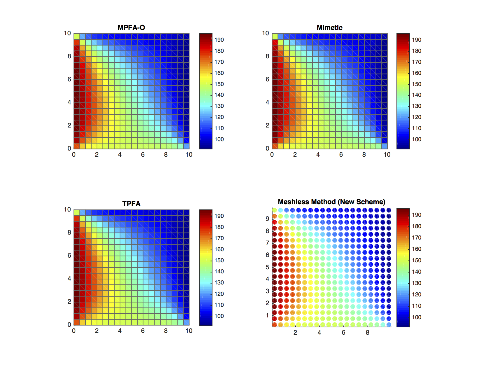
Refer to caption
Figure 8. Comparison of solutions of the Dirichlet problem for the Laplace equation. The method used are MPFA-O, Mimetic, TPFA, and Meshless methods (New Method: (44)–(46)).

5.1. Inhomogeneous Boundary Condition

Firstly, the homogeneous properties of the porous media 𝐌(𝒓)=𝐈𝐌𝒓𝐈\mathbf{M}\left(\boldsymbol{r}\right)=\mathbf{I} are assumed for simplicity of the derivation. The analytical solution of (1) subject to the assumption that g(𝒓)0𝑔𝒓0g\left(\boldsymbol{r}\right)\equiv 0 for 𝒓Ω2𝒓Ωsuperscript2\boldsymbol{r}\in\Omega\subset\mathbb{R}^{2} and constant boundary conditions is the following:

𝐮(x,y)=n=odd[4ψ1nπsinh(nπHL)]sin(nπLx)sinh(nπL(Hy))++n=odd[4ψ2nπsinh(nπLH)]sin(nπHy)sinh(nπHx)++n=odd[4ψ3nπsinh(nπLH)]sin(nπHy)sinh(nπHx)++n=odd[4ψ4nπsinh(nπLH)]sin(nπHy)sinh(nπH(Lx)),𝐮𝑥𝑦limit-fromsubscript𝑛𝑜𝑑𝑑delimited-[]4subscript𝜓1𝑛𝜋𝑛𝜋𝐻𝐿𝑛𝜋𝐿𝑥𝑛𝜋𝐿𝐻𝑦missing-subexpressionmissing-subexpressionlimit-fromsubscript𝑛𝑜𝑑𝑑delimited-[]4subscript𝜓2𝑛𝜋𝑛𝜋𝐿𝐻𝑛𝜋𝐻𝑦𝑛𝜋𝐻𝑥missing-subexpressionmissing-subexpressionlimit-fromsubscript𝑛𝑜𝑑𝑑delimited-[]4subscript𝜓3𝑛𝜋𝑛𝜋𝐿𝐻𝑛𝜋𝐻𝑦𝑛𝜋𝐻𝑥missing-subexpressionmissing-subexpressionsubscript𝑛𝑜𝑑𝑑delimited-[]4subscript𝜓4𝑛𝜋𝑛𝜋𝐿𝐻𝑛𝜋𝐻𝑦𝑛𝜋𝐻𝐿𝑥missing-subexpressionmissing-subexpression\begin{array}[]{lcl}\vspace{0.3cm}\displaystyle\mathbf{u}\left(x,y\right)=\sum\limits_{n=odd}\left[\frac{4\psi_{1}}{n\pi\sinh\left(\frac{n\pi H}{L}\right)}\right]\sin\left(\frac{n\pi}{L}x\right)\sinh\left(\frac{n\pi}{L}\left(H-y\right)\right)+\\ \vspace{0.3cm}\displaystyle+\sum\limits_{n=odd}\left[\frac{4\psi_{2}}{n\pi\sinh\left(\frac{n\pi L}{H}\right)}\right]\sin\left(\frac{n\pi}{H}y\right)\sinh\left(\frac{n\pi}{H}x\right)+\\ \vspace{0.3cm}\displaystyle+\sum\limits_{n=odd}\left[\frac{4\psi_{3}}{n\pi\sinh\left(\frac{n\pi L}{H}\right)}\right]\sin\left(\frac{n\pi}{H}y\right)\sinh\left(\frac{n\pi}{H}x\right)+\\ \displaystyle+\sum\limits_{n=odd}\left[\frac{4\psi_{4}}{n\pi\sinh\left(\frac{n\pi L}{H}\right)}\right]\sin\left(\frac{n\pi}{H}y\right)\sinh\left(\frac{n\pi}{H}\left(L-x\right)\right),\end{array} (58)

where ψ1subscript𝜓1\psi_{1} is the boundary at y=0𝑦0y=0, ψ2subscript𝜓2\psi_{2} at x=L𝑥𝐿x=L, ψ3subscript𝜓3\psi_{3} at y=H𝑦𝐻y=H, and ψ4subscript𝜓4\psi_{4} at x=0𝑥0x=0.

Tables 1, 2 shows the convergence rate of different schemes for uniform particle distribution. The solutions with MPFA and Mimetic schemes were obtained using MATLAB Reservoir Simulation Toolbox (MRST) [52]. It is clear from the convergence results that schemes (31)–(34) and (44)–(46) are identical and they overperform the scheme (30). The convergence rate as was predicted theoretically is at least 𝒪(hω), 1ω2𝒪superscript𝜔1𝜔2\mathcal{O}\left(h^{\omega}\right),\ 1\leq\omega\leq 2.

Table 1. The error of convergence for different schemes (uniform particle distribution) and f=0.5005𝑓0.5005f=0.5005.
DoF MPFA Mimetic Brookshaw (30) Schwaiger (31)–(34) New Scheme (44)–(46)
25 1.3181011.318superscript1011.318\cdot 10^{-1} 1.2401011.240superscript1011.240\cdot 10^{-1} 1.3141001.314superscript1001.314\cdot 10^{0} 6.6081026.608superscript1026.608\cdot 10^{-2} 6.6081026.608superscript1026.608\cdot 10^{-2}
100 3.2961023.296superscript1023.296\cdot 10^{-2} 3.0781023.078superscript1023.078\cdot 10^{-2} 3.9251013.925superscript1013.925\cdot 10^{-1} 1.8651021.865superscript1021.865\cdot 10^{-2} 1.8651021.865superscript1021.865\cdot 10^{-2}
400 8.2331038.233superscript1038.233\cdot 10^{-3} 7.6851037.685superscript1037.685\cdot 10^{-3} 1.1051011.105superscript1011.105\cdot 10^{-1} 4.7141034.714superscript1034.714\cdot 10^{-3} 4.7141034.714superscript1034.714\cdot 10^{-3}
1600 2.0581032.058superscript1032.058\cdot 10^{-3} 1.9201031.920superscript1031.920\cdot 10^{-3} 3.0251023.025superscript1023.025\cdot 10^{-2} 1.1791031.179superscript1031.179\cdot 10^{-3} 1.1791031.179superscript1031.179\cdot 10^{-3}
6400 5.3181045.318superscript1045.318\cdot 10^{-4} 4.9681044.968superscript1044.968\cdot 10^{-4} 8.1521038.152superscript1038.152\cdot 10^{-3} 3.2131043.213superscript1043.213\cdot 10^{-4} 3.2131043.213superscript1043.213\cdot 10^{-4}
25600 3.0071043.007superscript1043.007\cdot 10^{-4} 2.9551042.955superscript1042.955\cdot 10^{-4} 2.1931032.193superscript1032.193\cdot 10^{-3} 2.8071042.807superscript1042.807\cdot 10^{-4} 2.8071042.807superscript1042.807\cdot 10^{-4}
Table 2. The error of convergence for different schemes (uniformed particle distribution) and f=1.001𝑓1.001f=1.001.
DoF Brookshaw (30) Schwaiger (31)–(34) New Scheme (44)–(46)
25 2.3121012.312superscript1012.312\cdot 10^{-1} 1.0911011.091superscript1011.091\cdot 10^{-1} 1.0911011.091superscript1011.091\cdot 10^{-1}
100 1.1201011.120superscript1011.120\cdot 10^{-1} 2.6981022.698superscript1022.698\cdot 10^{-2} 2.6981022.698superscript1022.698\cdot 10^{-2}
400 3.9981023.998superscript1023.998\cdot 10^{-2} 6.7371036.737superscript1036.737\cdot 10^{-3} 6.7371036.737superscript1036.737\cdot 10^{-3}
1600 1.2621021.262superscript1021.262\cdot 10^{-2} 1.6841031.684superscript1031.684\cdot 10^{-3} 1.6841031.684superscript1031.684\cdot 10^{-3}
6400 3.7371033.737superscript1033.737\cdot 10^{-3} 4.4181044.418superscript1044.418\cdot 10^{-4} 4.4181044.418superscript1044.418\cdot 10^{-4}
25600 1.0971031.097superscript1031.097\cdot 10^{-3} 2.9191042.919superscript1042.919\cdot 10^{-4} 2.9191042.919superscript1042.919\cdot 10^{-4}

Tables 3, 4 shows the convergence rate for different schemes and pseudo random distribution. The reason for starting from f=0.5005𝑓0.5005f=0.5005 is that we want to force the same number of non-zero entries in the matrix as for MPFA or Memetic methods. This procedure may lead to a badly conditioned matrix since W¯(𝒓J𝒓I,h)1much-less-than¯𝑊subscript𝒓𝐽subscript𝒓𝐼1\overline{\nabla W}\left(\boldsymbol{r}_{J}-\boldsymbol{r}_{I},h\right)\ll 1. This distribution of particles was generated by perturbing the regularly distributed particles using a uniform random variable varying between +10%percent10+10\% and 10%percent10-10\% of the maximum smoothing length hmax=1.001subscript𝑚𝑎𝑥1.001h_{max}=1.001. Since random realizations are used to compute errors, the statistical data about 30 realizations are used to compute mean values and standard deviations. This data is presented in Tables 3, 4. The positive trends of the scheme remain the same as for the case of uniform particle distributions. The scheme (30) has higher error compare to schemes (31)–(34) and (44)–(46). However, the dispersion of the approximation error is higher in the scheme (44)–(46).

Table 3. The error of convergence for different schemes (random particle distribution) and f=0.6006𝑓0.6006f=0.6006.
DoF Brookshaw (30) Schwaiger (31)–(34) New Scheme (44)–(46)
25 1.10210+0±1.966102plus-or-minus1.102superscript1001.966superscript1021.102\cdot 10^{+0}\pm 1.966\cdot 10^{-2} 1.940101±3.954102plus-or-minus1.940superscript1013.954superscript1021.940\cdot 10^{-1}\pm 3.954\cdot 10^{-2} 3.707101±1.319101plus-or-minus3.707superscript1011.319superscript1013.707\cdot 10^{-1}\pm 1.319\cdot 10^{-1}
100 3.361101±4.923103plus-or-minus3.361superscript1014.923superscript1033.361\cdot 10^{-1}\pm 4.923\cdot 10^{-3} 5.511102±1.205102plus-or-minus5.511superscript1021.205superscript1025.511\cdot 10^{-2}\pm 1.205\cdot 10^{-2} 9.074102±2.668102plus-or-minus9.074superscript1022.668superscript1029.074\cdot 10^{-2}\pm 2.668\cdot 10^{-2}
400 9.576102±8.705104plus-or-minus9.576superscript1028.705superscript1049.576\cdot 10^{-2}\pm 8.705\cdot 10^{-4} 1.376102±2.440103plus-or-minus1.376superscript1022.440superscript1031.376\cdot 10^{-2}\pm 2.440\cdot 10^{-3} 2.299102±6.972103plus-or-minus2.299superscript1026.972superscript1032.299\cdot 10^{-2}\pm 6.972\cdot 10^{-3}
1600 2.640102±2.551104plus-or-minus2.640superscript1022.551superscript1042.640\cdot 10^{-2}\pm 2.551\cdot 10^{-4} 4.157103±7.485104plus-or-minus4.157superscript1037.485superscript1044.157\cdot 10^{-3}\pm 7.485\cdot 10^{-4} 5.912103±1.289103plus-or-minus5.912superscript1031.289superscript1035.912\cdot 10^{-3}\pm 1.289\cdot 10^{-3}
6400 7.185103±5.982105plus-or-minus7.185superscript1035.982superscript1057.185\cdot 10^{-3}\pm 5.982\cdot 10^{-5} 1.044103±1.465104plus-or-minus1.044superscript1031.465superscript1041.044\cdot 10^{-3}\pm 1.465\cdot 10^{-4} 1.406103±3.090104plus-or-minus1.406superscript1033.090superscript1041.406\cdot 10^{-3}\pm 3.090\cdot 10^{-4}
25600 1.944103±1.451105plus-or-minus1.944superscript1031.451superscript1051.944\cdot 10^{-3}\pm 1.451\cdot 10^{-5} 3.858104±5.887105plus-or-minus3.858superscript1045.887superscript1053.858\cdot 10^{-4}\pm 5.887\cdot 10^{-5} 4.960104±8.425105plus-or-minus4.960superscript1048.425superscript1054.960\cdot 10^{-4}\pm 8.425\cdot 10^{-5}
Table 4. The error of convergence for different schemes (random particle distribution) and f=1.2012𝑓1.2012f=1.2012.
DoF Brookshaw (30) Schwaiger (31)–(34) New Scheme (44)–(46)
25 3.578101±2.879102plus-or-minus3.578superscript1012.879superscript1023.578\cdot 10^{-1}\pm 2.879\cdot 10^{-2} 2.162101±2.800102plus-or-minus2.162superscript1012.800superscript1022.162\cdot 10^{-1}\pm 2.800\cdot 10^{-2} 1.842101±8.871103plus-or-minus1.842superscript1018.871superscript1031.842\cdot 10^{-1}\pm 8.871\cdot 10^{-3}
100 1.261101±4.859103plus-or-minus1.261superscript1014.859superscript1031.261\cdot 10^{-1}\pm 4.859\cdot 10^{-3} 5.696102±5.518103plus-or-minus5.696superscript1025.518superscript1035.696\cdot 10^{-2}\pm 5.518\cdot 10^{-3} 4.596102±1.999103plus-or-minus4.596superscript1021.999superscript1034.596\cdot 10^{-2}\pm 1.999\cdot 10^{-3}
400 4.224102±1.092103plus-or-minus4.224superscript1021.092superscript1034.224\cdot 10^{-2}\pm 1.092\cdot 10^{-3} 1.493102±1.546103plus-or-minus1.493superscript1021.546superscript1031.493\cdot 10^{-2}\pm 1.546\cdot 10^{-3} 1.157102±5.691104plus-or-minus1.157superscript1025.691superscript1041.157\cdot 10^{-2}\pm 5.691\cdot 10^{-4}
1600 1.299102±2.031104plus-or-minus1.299superscript1022.031superscript1041.299\cdot 10^{-2}\pm 2.031\cdot 10^{-4} 3.934103±3.969104plus-or-minus3.934superscript1033.969superscript1043.934\cdot 10^{-3}\pm 3.969\cdot 10^{-4} 2.889103±1.451104plus-or-minus2.889superscript1031.451superscript1042.889\cdot 10^{-3}\pm 1.451\cdot 10^{-4}
6400 3.862103±3.452105plus-or-minus3.862superscript1033.452superscript1053.862\cdot 10^{-3}\pm 3.452\cdot 10^{-5} 1.037103±8.443105plus-or-minus1.037superscript1038.443superscript1051.037\cdot 10^{-3}\pm 8.443\cdot 10^{-5} 7.507104±4.060105plus-or-minus7.507superscript1044.060superscript1057.507\cdot 10^{-4}\pm 4.060\cdot 10^{-5}
25600 1.133103±2.125105plus-or-minus1.133superscript1032.125superscript1051.133\cdot 10^{-3}\pm 2.125\cdot 10^{-5} 4.087104±5.405105plus-or-minus4.087superscript1045.405superscript1054.087\cdot 10^{-4}\pm 5.405\cdot 10^{-5} 3.475104±3.814105plus-or-minus3.475superscript1043.814superscript1053.475\cdot 10^{-4}\pm 3.814\cdot 10^{-5}

Figure 8 shows the numerical solution of the boundary value problem obtained using different discretization methods. The solution was obtained using 40 particles/cells in each direction.

5.2. Inhomogeneous Mixed Boundary Condition Test

The general steady-state solution for a Dirichlet condition along the base of the plate and Neumann conditions elsewhere is given in [2] by

𝐮(x,y)=ψ1+ψ3y+n=12ψ2cosh(λnx)+2ψ4cosh(λn(Lx))Hλn2sinh(λnL)sinh(λny),𝐮𝑥𝑦subscript𝜓1subscript𝜓3𝑦subscriptsuperscript𝑛12subscript𝜓2subscript𝜆𝑛𝑥2subscript𝜓4subscript𝜆𝑛𝐿𝑥𝐻subscriptsuperscript𝜆2𝑛subscript𝜆𝑛𝐿subscript𝜆𝑛𝑦\displaystyle\mathbf{u}\left(x,y\right)=\psi_{1}+\psi_{3}y+\sum\limits^{\infty}_{n=1}\frac{2\psi_{2}\cosh\left(\lambda_{n}x\right)+2\psi_{4}\cosh\left(\lambda_{n}\left(L-x\right)\right)}{H\lambda^{2}_{n}\sinh\left(\lambda_{n}L\right)}\sinh\left(\lambda_{n}y\right), (59)

where ψ1subscript𝜓1\psi_{1} is the boundary value of 𝐮𝐮\mathbf{u} at y=0𝑦0y=0, ψ2subscript𝜓2\psi_{2} is the flux at x=L𝑥𝐿x=L, ψ3subscript𝜓3\psi_{3} is the flux at y=H𝑦𝐻y=H, and ψ4subscript𝜓4\psi_{4} is the flux at x=0𝑥0x=0, and λn=(2n1)π2Hsubscript𝜆𝑛2𝑛1𝜋2𝐻\displaystyle\lambda_{n}=\frac{\left(2n-1\right)\pi}{2H}. The following parameters (dimensionless) were chosen:ψ1=150subscript𝜓1150\psi_{1}=150, ψ3=150subscript𝜓3150\psi_{3}=150, ψ4=200subscript𝜓4200\psi_{4}=200, ψ2=90subscript𝜓290\psi_{2}=90. Again, for uniform and regular particles distribution, MPFA method reduces to the TPFA. Similar to the previous section, the regular and pseudo random particle distribution are considered to access the convergence properties of the proposed schemes.

Remark 4.

Let ΓN=subscriptΓ𝑁\Gamma_{N}=\varnothing and ΓD=subscriptΓ𝐷\Gamma_{D}=\varnothing, g(𝐫)0,𝐫Ωformulae-sequence𝑔𝐫0𝐫Ωg\left(\boldsymbol{r}\right)\geq 0,\ \boldsymbol{r}\in\Omega, gN(𝐫)0,𝐫ΓNformulae-sequencesubscript𝑔𝑁𝐫0𝐫subscriptΓ𝑁g_{N}\left(\boldsymbol{r}\right)\geq 0,\ \boldsymbol{r}\in\Gamma_{N}, gD(𝐫)0,𝐫ΓDformulae-sequencesubscript𝑔𝐷𝐫0𝐫subscriptΓ𝐷g_{D}\left(\boldsymbol{r}\right)\geq 0,\ \boldsymbol{r}\in\Gamma_{D} and the solution of

𝐋(𝐮)=0,or(𝐌(𝒓)𝐮(𝒓))=g(𝒓),𝒓Ωn,formulae-sequence𝐋𝐮0orformulae-sequence𝐌𝒓𝐮𝒓𝑔𝒓for-all𝒓Ωsuperscript𝑛\displaystyle\vspace{0.2cm}\mathbf{L}\left(\mathbf{u}\right)=0,\ \mbox{or}\ \ \ \nabla\left(\mathbf{M}\left(\boldsymbol{r}\right)\nabla\mathbf{u}\left(\boldsymbol{r}\right)\right)=g\left(\boldsymbol{r}\right),\ \forall\boldsymbol{r}\in\Omega\subset\mathbb{R}^{n}, (60)

exists then it can be discretized in all internal particles by the following schemes Brookshaw (30), Schwaiger (31)–(34), and New Scheme (44)–(46) and compounded with the following condition for all 𝐫ΓN𝐫subscriptΓ𝑁\boldsymbol{r}\in\Gamma_{N}:

𝒖α𝒏α=𝒏α𝐌αβ(𝒓)Ω𝒓,h~V𝒓J[𝐮(𝒓J)𝐮(𝒓I)]βW¯(𝒓J𝒓I,h)delimited-⟨⟩superscript𝒖𝛼subscript𝒏𝛼subscript𝒏𝛼superscript𝐌𝛼𝛽𝒓subscriptsubscriptΩ𝒓~subscript𝑉subscript𝒓𝐽delimited-[]𝐮subscript𝒓𝐽𝐮subscript𝒓𝐼¯subscriptsuperscript𝛽𝑊subscript𝒓𝐽subscript𝒓𝐼\langle\boldsymbol{u}^{\alpha}\boldsymbol{n}_{\alpha}\rangle=\boldsymbol{n}_{\alpha}\mathbf{M}^{\alpha\beta}\left(\boldsymbol{r}\right)\sum\limits_{\Omega_{\boldsymbol{r},\tilde{h}}}V_{\boldsymbol{r}_{J}}\left[\mathbf{u}\left(\boldsymbol{r}_{J}\right)-\mathbf{u}\left(\boldsymbol{r}_{I}\right)\right]\overline{\nabla^{*}_{\beta}W}\left(\boldsymbol{r}_{J}-\boldsymbol{r}_{I},h\right) (61)

where 𝐧αsubscript𝐧𝛼\boldsymbol{n}_{\alpha} are the component of the external normal to the boundary 𝐫ΓN𝐫subscriptΓ𝑁\boldsymbol{r}\in\Gamma_{N}.

The following smoothing multiplication factors f=0.5005𝑓0.5005f=0.5005, f=1.001𝑓1.001f=1.001, and f=2.002𝑓2.002f=2.002 are considered. Tables 5, 6 show the convergence rate for different schemes using the uniform and pseudo random particle distribution. The convergence rate as was predicted theoretically is at least 𝒪(hω), 1ω<2𝒪superscript𝜔1𝜔2\mathcal{O}\left(h^{\omega}\right),\ 1\leq\omega<2. Interestingly, the scheme (30) shows a very bad convergence rate for f=0.5005𝑓0.5005f=0.5005. This explains by the fact that we have one particle from each side in the kernel support almost next to the boundary of the kernel support leading to W¯(𝒓J𝒓I,h)1much-less-than¯𝑊subscript𝒓𝐽subscript𝒓𝐼1\overline{\nabla W}\left(\boldsymbol{r}_{J}-\boldsymbol{r}_{I},h\right)\ll 1 and, hence, to a badly conditioned matrix. This does not observed for other schemes due to the normalization coefficient. As a result, the scheme (30) should be used with more than one particle in the compact support in each direction leading to a larger bandwidth in the matrix.

Table 5. The error of convergence for different schemes (uniform particle distribution) and f=0.5005𝑓0.5005f=0.5005.
DoF MPFA Mimetic Brookshaw (30) Schwaiger (31)–(34) New Scheme (44)–(46)
25 1.4891011.489superscript1011.489\cdot 10^{-1} 2.6511022.651superscript1022.651\cdot 10^{-2} 1.4891061.489superscript1061.489\cdot 10^{6} 8.2441018.244superscript1018.244\cdot 10^{-1} 8.2441018.244superscript1018.244\cdot 10^{-1}
100 2.0151022.015superscript1022.015\cdot 10^{-2} 4.4241034.424superscript1034.424\cdot 10^{-3} 9.4711059.471superscript1059.471\cdot 10^{5} 2.1781012.178superscript1012.178\cdot 10^{-1} 2.1781012.178superscript1012.178\cdot 10^{-1}
400 2.7271032.727superscript1032.727\cdot 10^{-3} 6.8891046.889superscript1046.889\cdot 10^{-4} 5.3781055.378superscript1055.378\cdot 10^{5} 5.5501025.550superscript1025.550\cdot 10^{-2} 5.5501025.550superscript1025.550\cdot 10^{-2}
1600 3.6661043.666superscript1043.666\cdot 10^{-4} 1.0241041.024superscript1041.024\cdot 10^{-4} 2.8591052.859superscript1052.859\cdot 10^{5} 1.3981021.398superscript1021.398\cdot 10^{-2} 1.3981021.398superscript1021.398\cdot 10^{-2}
6400 4.9511054.951superscript1054.951\cdot 10^{-5} 1.5221051.522superscript1051.522\cdot 10^{-5} 1.4731051.473superscript1051.473\cdot 10^{5} 3.5041033.504superscript1033.504\cdot 10^{-3} 3.5041033.504superscript1033.504\cdot 10^{-3}
25600 7.3091067.309superscript1067.309\cdot 10^{-6} 2.9201062.920superscript1062.920\cdot 10^{-6} 7.4741047.474superscript1047.474\cdot 10^{4} 8.7701048.770superscript1048.770\cdot 10^{-4} 8.7701048.770superscript1048.770\cdot 10^{-4}
Table 6. The error of convergence for different schemes (uniform particle distribution) and f=1.001𝑓1.001f=1.001.
DoF Brookshaw (30) Schwaiger (31)–(34) New Scheme (44)–(46)
25 1.1631001.163superscript1001.163\cdot 10^{0} 1.0781011.078superscript1011.078\cdot 10^{-1} 1.0781011.078superscript1011.078\cdot 10^{-1}
100 1.2081001.208superscript1001.208\cdot 10^{0} 1.4881021.488superscript1021.488\cdot 10^{-2} 1.4881021.488superscript1021.488\cdot 10^{-2}
400 8.2911018.291superscript1018.291\cdot 10^{-1} 2.2441032.244superscript1032.244\cdot 10^{-3} 2.2441032.244superscript1032.244\cdot 10^{-3}
1600 4.8311014.831superscript1014.831\cdot 10^{-1} 4.2151044.215superscript1044.215\cdot 10^{-4} 4.2151044.215superscript1044.215\cdot 10^{-4}
6400 2.6061012.606superscript1012.606\cdot 10^{-1} 9.8581059.858superscript1059.858\cdot 10^{-5} 9.8581059.858superscript1059.858\cdot 10^{-5}
25600 1.3531011.353superscript1011.353\cdot 10^{-1} 2.5021052.502superscript1052.502\cdot 10^{-5} 2.5021052.502superscript1052.502\cdot 10^{-5}

Tables 7, 8 show the convergence rate for different schemes with pseudo random particle distribution. The pseudo random distribution of particles was again generated by perturbing the regularly distributed particles using the uniform random variable varying between +10%percent10+10\% and 10%percent10-10\% of the maximum smoothing length hmax=1.001subscript𝑚𝑎𝑥1.001h_{max}=1.001. Similar to the above case, the statistical data about 30 realizations are used to compute mean values and standard deviations. These data are presented in Tables 7, 8. The general trends of the scheme prosperities remain the same as for uniform particle distributions. The scheme (30) has higher error compared to schemes (31)–(34) and (44)–(46). However, the dispersion of the approximation error is higher in the scheme (44)–(46).

Table 7. The error of convergence for different schemes (random particle distribution) and f=0.6006𝑓0.6006f=0.6006.
DoF Brookshaw (30) Schwaiger (31)–(34) New Scheme (44)–(46)
25 5.608101±1.019100plus-or-minus5.608superscript1011.019superscript1005.608\cdot 10^{1}\pm 1.019\cdot 10^{0} 8.815101±4.248101plus-or-minus8.815superscript1014.248superscript1018.815\cdot 10^{-1}\pm 4.248\cdot 10^{-1} 1.242100±5.058101plus-or-minus1.242superscript1005.058superscript1011.242\cdot 10^{0}\pm 5.058\cdot 10^{-1}
100 3.769101±5.708101plus-or-minus3.769superscript1015.708superscript1013.769\cdot 10^{1}\pm 5.708\cdot 10^{-1} 3.454101±1.977101plus-or-minus3.454superscript1011.977superscript1013.454\cdot 10^{-1}\pm 1.977\cdot 10^{-1} 4.361101±2.425101plus-or-minus4.361superscript1012.425superscript1014.361\cdot 10^{-1}\pm 2.425\cdot 10^{-1}
400 2.154101±1.757101plus-or-minus2.154superscript1011.757superscript1012.154\cdot 10^{1}\pm 1.757\cdot 10^{-1} 8.454102±5.111102plus-or-minus8.454superscript1025.111superscript1028.454\cdot 10^{-2}\pm 5.111\cdot 10^{-2} 1.525101±1.195101plus-or-minus1.525superscript1011.195superscript1011.525\cdot 10^{-1}\pm 1.195\cdot 10^{-1}
1600 1.159101±7.457102plus-or-minus1.159superscript1017.457superscript1021.159\cdot 10^{1}\pm 7.457\cdot 10^{-2} 2.245102±1.055102plus-or-minus2.245superscript1021.055superscript1022.245\cdot 10^{-2}\pm 1.055\cdot 10^{-2} 4.563102±2.328102plus-or-minus4.563superscript1022.328superscript1024.563\cdot 10^{-2}\pm 2.328\cdot 10^{-2}
6400 6.027100±2.312102plus-or-minus6.027superscript1002.312superscript1026.027\cdot 10^{0}\pm 2.312\cdot 10^{-2} 1.104102±7.523103plus-or-minus1.104superscript1027.523superscript1031.104\cdot 10^{-2}\pm 7.523\cdot 10^{-3} 1.848102±9.276103plus-or-minus1.848superscript1029.276superscript1031.848\cdot 10^{-2}\pm 9.276\cdot 10^{-3}
25600 3.054100±1.174102plus-or-minus3.054superscript1001.174superscript1023.054\cdot 10^{0}\pm 1.174\cdot 10^{-2} 4.123103±2.059103plus-or-minus4.123superscript1032.059superscript1034.123\cdot 10^{-3}\pm 2.059\cdot 10^{-3} 5.879103±4.253103plus-or-minus5.879superscript1034.253superscript1035.879\cdot 10^{-3}\pm 4.253\cdot 10^{-3}
Table 8. The error of convergence for different schemes (random particle distribution) and f=1.2012𝑓1.2012f=1.2012.
DoF Brookshaw (30) Schwaiger (31)–(34) New Scheme (44)–(46)
25 5.177101±7.312102plus-or-minus5.177superscript1017.312superscript1025.177\cdot 10^{-1}\pm 7.312\cdot 10^{-2} 3.143101±7.543102plus-or-minus3.143superscript1017.543superscript1023.143\cdot 10^{-1}\pm 7.543\cdot 10^{-2} 4.302101±1.461101plus-or-minus4.302superscript1011.461superscript1014.302\cdot 10^{-1}\pm 1.461\cdot 10^{-1}
100 5.160101±4.035102plus-or-minus5.160superscript1014.035superscript1025.160\cdot 10^{-1}\pm 4.035\cdot 10^{-2} 5.959102±4.713103plus-or-minus5.959superscript1024.713superscript1035.959\cdot 10^{-2}\pm 4.713\cdot 10^{-3} 1.106101±1.739102plus-or-minus1.106superscript1011.739superscript1021.106\cdot 10^{-1}\pm 1.739\cdot 10^{-2}
400 4.349101±1.715102plus-or-minus4.349superscript1011.715superscript1024.349\cdot 10^{-1}\pm 1.715\cdot 10^{-2} 1.515102±1.973103plus-or-minus1.515superscript1021.973superscript1031.515\cdot 10^{-2}\pm 1.973\cdot 10^{-3} 3.015102±1.045102plus-or-minus3.015superscript1021.045superscript1023.015\cdot 10^{-2}\pm 1.045\cdot 10^{-2}
1600 2.745101±9.059103plus-or-minus2.745superscript1019.059superscript1032.745\cdot 10^{-1}\pm 9.059\cdot 10^{-3} 3.926103±6.865104plus-or-minus3.926superscript1036.865superscript1043.926\cdot 10^{-3}\pm 6.865\cdot 10^{-4} 1.133102±5.486103plus-or-minus1.133superscript1025.486superscript1031.133\cdot 10^{-2}\pm 5.486\cdot 10^{-3}
6400 1.508101±2.822103plus-or-minus1.508superscript1012.822superscript1031.508\cdot 10^{-1}\pm 2.822\cdot 10^{-3} 1.595103±8.144104plus-or-minus1.595superscript1038.144superscript1041.595\cdot 10^{-3}\pm 8.144\cdot 10^{-4} 3.187103±1.438103plus-or-minus3.187superscript1031.438superscript1033.187\cdot 10^{-3}\pm 1.438\cdot 10^{-3}
25600 7.958102±1.146103plus-or-minus7.958superscript1021.146superscript1037.958\cdot 10^{-2}\pm 1.146\cdot 10^{-3} 5.354104±2.036104plus-or-minus5.354superscript1042.036superscript1045.354\cdot 10^{-4}\pm 2.036\cdot 10^{-4} 9.201104±5.201104plus-or-minus9.201superscript1045.201superscript1049.201\cdot 10^{-4}\pm 5.201\cdot 10^{-4}

Results of the numerical solution are compared with the series solution in Figure 11.
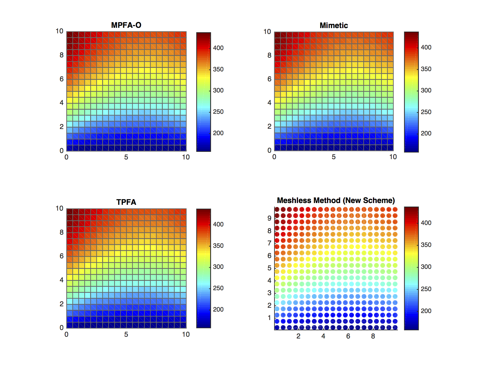
Refer to caption
Figure 9. Comparison of solutions of the inhomogeneous mixed boundary problems for the Laplace equations. The method used are MPFA-O, Mimetic, TPFA, and Meshless methods (New Method: (44)–(46)).

5.3. SPE10

In addition, we investigate the accuracy of the numerical schemes using a well-known SPE10 benchmark [53] with the Laplace equation:

𝐋(𝐮)=(𝐌(𝒓)𝐮(𝒓))=0,𝒓Ωn,𝐌αβ(𝒓)=Kαβ(𝒓),Kαβ(𝒓)=0αβ;α,β=1,,n;formulae-sequence𝐋𝐮𝐌𝒓𝐮𝒓0for-all𝒓Ωsuperscript𝑛missing-subexpressionmissing-subexpressionformulae-sequenceformulae-sequencesuperscript𝐌𝛼𝛽𝒓superscript𝐾𝛼𝛽𝒓superscript𝐾𝛼𝛽𝒓0for-all𝛼𝛽𝛼𝛽1𝑛missing-subexpressionmissing-subexpression\begin{array}[]{lcl}\displaystyle\vspace{0.2cm}\mathbf{L}\left(\mathbf{u}\right)=-\nabla\left(\mathbf{M}\left(\boldsymbol{r}\right)\nabla\mathbf{u}\left(\boldsymbol{r}\right)\right)=0,\ \forall\boldsymbol{r}\in\Omega\subset\mathbb{R}^{n},\\ \mathbf{M}^{\alpha\beta}\left(\boldsymbol{r}\right)=K^{\alpha\beta}\left(\boldsymbol{r}\right),\ K^{\alpha\beta}\left(\boldsymbol{r}\right)=0\ \forall\alpha\neq\beta;\ \alpha,\beta=1,\ldots,n;\end{array} (62)

where 𝐮(𝒓)𝐮𝒓\mathbf{u}\left(\boldsymbol{r}\right) is the unknown pressure field, Kαβ(𝒓)superscript𝐾𝛼𝛽𝒓K^{\alpha\beta}\left(\boldsymbol{r}\right) is the diagonal permeability field. The original model contains 85 layers, where layers from 1 to 35 have smooth permeability with lognormal distribution and layers 36 to 85 have channelized formations that are considered to be significantly more challenging for numerical simulations. The subset of this model is defined by the global Cartesian indices I𝐼I, J𝐽J, K𝐾K. The 85 layer was used as a permeability field for 2D simulation with Cartesian indices I=1:60:𝐼160I=1:60 and J=1:60:𝐽160J=1:60. In 3D, the subsection Cartesian indices I=1:60:𝐼160I=1:60, J=1:60:𝐽160J=1:60, and K=1:60:𝐾160K=1:60. The permeability fields K11superscript𝐾11K^{11} for both cases are shown in Figure 10.
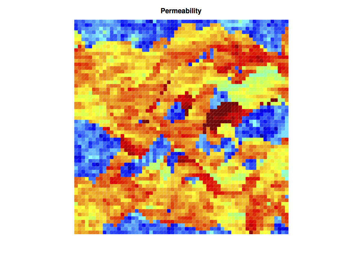
Refer to caption Case (a)          Refer to caption Case (b)

Figure 10. The lognormal permeability field in the SPE10 benchmark test. Case (a) 60×60606060\times 60cells of 85 layer. Case (b) subsection of the SPE10 model defined by 60×60×6060606060\times 60\times 60 cells.

The boundary conditions correspond to the unit pressure drop over the entire domain in J𝐽J-direction (i.e., ymin=0subscript𝑦𝑚𝑖𝑛0y_{min}=0 and ymax=1subscript𝑦𝑚𝑎𝑥1y_{max}=1). The numerical results using new scheme for the SPE10 cases are presented in Figure 11. The relative error distribution is also shown for 2D and 3D cases, where the error is computed using (57) and numerical solution based on TPFA.
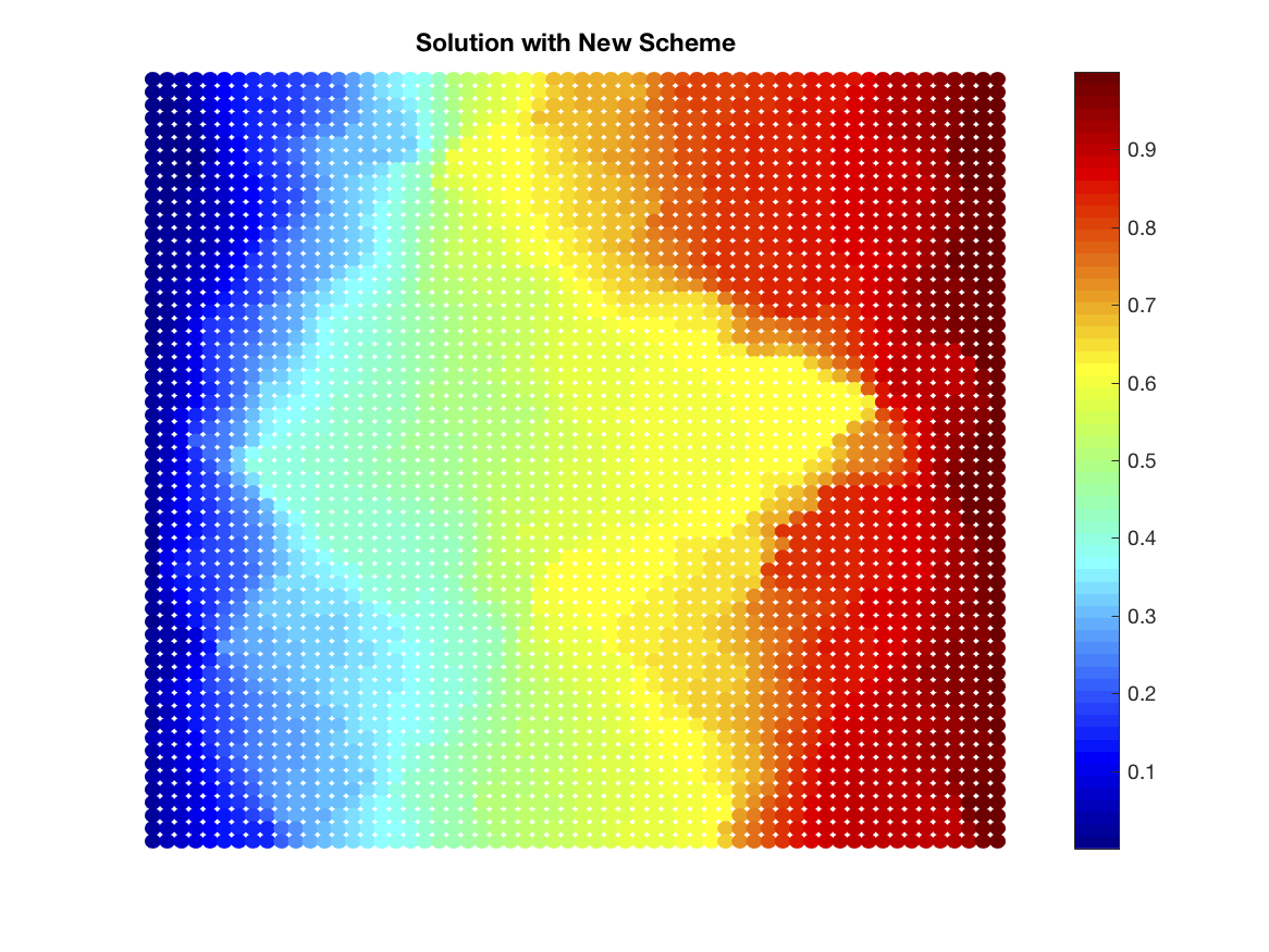
Refer to caption Numerical Solution (2D Case) Refer to caption Relative Error % (2D Case)
Refer to caption Numerical Solution (3D Case) Refer to caption Relative Error % (3D Case)

Figure 11. Numerical solution obtained with the new scheme for the SPE10 cases. The relative error distribution is also shown for 2D and 3D cases, where error is computed using (57) and numerical solution based on TPFA.

Figures 12 and 13 compare the convergence rates of the various discretizations subject to different preconditioners.
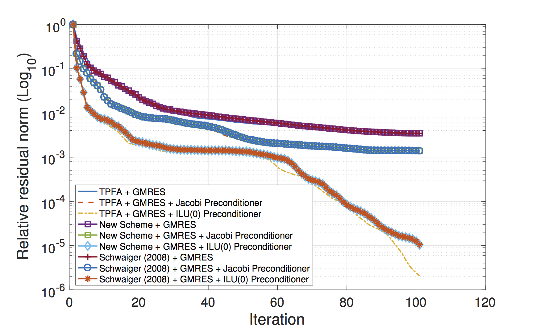
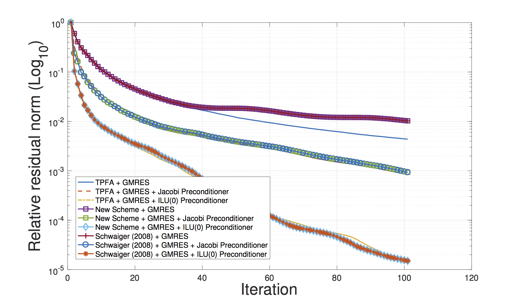
Refer to caption
Figure 12. Comparison of the convergence rate of the GMRES iterative method with and without preconditioner for different numerical discretization methods (TPFA, New Scheme (44)–(46), Schwaiger (31)–(34)). The linear system of equations is built using 2D case.
Refer to caption
Figure 13. Comparison of the convergence rate of the GMRES iterative method with and without preconditioner for different numerical discretization methods (TPFA, New Scheme (44)–(46), Schwaiger (31)–(34)). The linear system of equations is built using 3D case.

Furthermore, if we notice the convergence comparison for this test in Figures 12 and 13, the proposed new method offers similar convergence as compared to the Schwaiger’s scheme (31)–(34)). The reason for such convergence is the similarity between condition numbers of the linear system of equations resulting from these methods.

Another interesting observation in this numerical test is the small values of the relative error between the TPFA solution and proposed new method for both 2D and 3D cases. This observation exhibits the efficiency of the proposed meshless discretization scheme, which explains the higher accuracy of linear reproduction.

6. Conclusion

In this paper, the new stable SPH discretization of the elliptic operator for heterogeneous media is proposed. The scheme has the two-point flux approximation nature and can be written in the form of (2). Using this structure, it was possible to make some theoretical monotonicity analysis (see, Remarks 2 and 3), which is difficult to perform for other schemes (e.g., Schwaiger’s method). Furthermore, it follows from the Taylor’s series analysis that proposed scheme is the optimum one in this class (2) for a diagonal matrix of the operator coefficients. In addition, the proposed scheme allows to apply upwinding strategy during the solution of nonlinear PDEs.

The new scheme is based on a gradient approximation commonly used in thermal, viscous, and pressure projection problems and can be extended to include higher-order terms in the appropriate Taylor series. The proposed new scheme is combined with mixed corrections which ensure linear completeness. The mixed correction utilizes Shepard Functions in combination with a correction to derivative approximations. Incompleteness of the kernel support combined with the lack of consistency of the kernel interpolation in conventional meshless method results in fuzzy boundaries. In the presented meshless method, the domain boundary conditions and internal field variables are approximated with the default accuracy of the method. The resulting new scheme not only ensures first order accuracy 𝒪(hα), 1α2𝒪superscript𝛼1𝛼2\mathcal{O}(h^{\alpha}),\ 1\leq\alpha\leq 2, where hh denotes the maximum particle spacing, but also minimize the impact of the particle deficiency (kernel support incompleteness) problem.

Furthermore, different Kernel gradients and their impact on the property of the scheme and accuracy are discussed. The model was tested by solving an inhomogeneous Dirichlet and mixed boundary value problems for the Laplacian equation with good accuracy confirming our theoretical results. The accuracy of Schwaiger’s scheme and new scheme is the same for homogeneous particle distribution and different for the distorted particles. The new scheme takes into account all terms related to Hessian of the unknown function (see, relation (43)).

The stability analysis shows that von Neumann growth factor has both real and imaginary parts forming complex shape for general particle distribution but satisfying the stability requirement almost everywhere. The paper also discusses the monotonicity and convergence properties of the new proposed scheme and demonstrates that there is a parameter hh such that the proposed new scheme is unconditionally monotone with the scalar heterogeneous media.

As was previously mentioned in the introduction, several methods have been proposed to address the difficulties involved in calculating second-order derivatives with SPH. In contrast to the present formulation, many of these methods achieve a high accuracy through fully calculating the Hessian or requiring that the discrete equations exactly reproduce quadratic functions. The primary attraction of the present method is that it provides a weak formulation for Darcy’s law which can be of use in further development of meshless methods. The SPH model was previously used to model three-dimensional miscible flow and transport in porous media with complex geometry, and we are planning to use this model in future work for large (field) scale simulation of transport in porous media with general permeability distributions.

References

  • [1] L. Brookshaw. A method of calculating radiative heat diffusion in particle simulations. Proceedings of the Astronomical Society of Australia, 6(2):207–210, 1985.
  • [2] H.F. Schwaiger. An implicit corrected sph formulation for thermal diffusion with linear free surface boundary conditions. International Journal for Numerical Methods in Engineering, 75(6):647–671, 2008.
  • [3] L. Lucy. A numerical approach to testing the fission hypothesis. The Astronomical Journal, 82(12):1013–1024, 1977.
  • [4] R.A. Gingold and J.J. Monaghan. Smoothed particle hydrodynamics: theory and applications to non-spherical stars. Mon. Not. R. Astr. Soc., 181:375–389, 1977.
  • [5] R.A. Gingold and J.J. Monaghan. Kernel estimates as a basis for general particle methods in hydrodynamics. J. Comput. Phys., 46(3):429–453, 1982.
  • [6] J.J. Monaghan. Smoothed particle hydrodynamics. Annual Reviews in Astronomy and Astrophysics, 30:543–574, 1992.
  • [7] T. Belytschko, Y. Krongauz, J. Dolbow, and C. Gerlach. On the completeness of meshfree particle methods. Int. J. for Numerical Methods in Engineering, 43(5):785–819, 1998.
  • [8] J.W. Swegle, D.L. Hicks, and S.W. Attaway. Smoothed Particle Hydrodynamics stability analysis. J. Computational Physics, 116(1):123–134, 1995.
  • [9] T. Belytschko, Y. Guo, W.K. Liu, and S.P. Xiao. A unified stability analysis of meshless particle methods. Int. J. Numer. Meth. in Engng, 48(9):1359–1400, 2000.
  • [10] Ch. Zhang, X.Y. Hu, and N.A. Adams. A generalized transport-velocity formulation for smoothed particle hydrodynamics. Journal of Computational Physics, 337:216–232, 2017.
  • [11] A. Khayyer, H. Gotoh, and Y. Shimizu. Comparative study on accuracy and conservation properties of two particle regularization schemes and proposal of an optimized particle shifting scheme in isph context. Journal of Computational Physics, 332:236–256, 2017.
  • [12] M.B. Liu, G.R. Liu, and K.Y. Lam. Computer simulation of high explosive explosion using smoothed particle hydrodynamics methodology. Comput. Fluids, 32(3):305–322, 2003.
  • [13] A.A. Lukyanov. Numerical modelling of the material failure under shock loading using particle method. Izvetiya Tula State University. Estestvennonauchn. Ser., 1:54–65, 2007.
  • [14] A.A. Lukyanov and V.B. Penkov. Numerical simulation of solids deformation by a meshless method. Vestn. Samar. Gos. Univ. Estestvennonauchn. Ser., 6(56):62–70, 2007.
  • [15] J.J. Monaghan. Simulating free surface flows with SPH. Journal of Computational Physics, 110(2):399–406, 1994.
  • [16] G.R. Johnson, R.A. Stryk, and S.R. Beissel. SPH for high velocity impact computations. Computational Methods in Applied Mechanical Engineering, 139(1):347–373, 1996.
  • [17] J.K. Chen, J.E. Beraun, and C.J. Jih. Completeness of corrective smoothed particle method for linear elastodynamics. Computational Mechanics, 24(4):273–285, 1999.
  • [18] J.K. Chen, J.E. Beraun, and C.J. Jih. A corrective smoothed particle method for transient elastoplastic dynamics. Computational Mechanics, 27(3):177–187, 2001.
  • [19] J.P. Morris, P.J. Fox, and Y. Zhu. Modeling low Reynolds number incompressible flows using SPH. J. Comput. Phys., 136(1):214–226, 1997.
  • [20] D.W. Holmes, J.R. Williams, and P. Tilke. Smooth particle hydrodynamics simulations of low Reynolds number flows through porous media. International Journal for Numerical and Analytical Methods in Geomechanics, 35(4):419–437, 2010.
  • [21] Y. Zhu, P.J. Fox, and J.P. Morris. A pore-scale numerical model for flow through porous media. Int. J. Numer. Anal. Meth. Geomech., 23(9):881–904, 1999.
  • [22] Y. Zhu and P.J. Fox. Smoothed particle hydrodynamics model for diffusion through porous media. Transport Porous Media, 43(3):441–471, 2001.
  • [23] A.K. Chaniotis, D. Poulikakos, and P. Koumoutsakos. Remeshed smoothed particle hydrodynamics for the simulation of viscous and heat conduction flows. Journal of Computational Physics, 182(1):67–90, 2002.
  • [24] D.A. Fulk and D.W. Quinn. An analysis of 1-d Smoothed Particle Hydrodynamics kernels. J. of Computational Physics, 126(1):165–180, 1996.
  • [25] G.R. Liu and M.B. Liu. Smoothed Particle Hydrodynamics: A Meshfree Particle Method. World Scientific Publishing Co. Pte. Ltd., 2003.
  • [26] S. Li and W.K. Liu. Meshfree and particle methods and their applications. Applied Mechanics Review, 55(1):1–34, 2002.
  • [27] P. Breitkopf and A. Huerta. Meshless & Particle Based Approaches in Computational Mechanics. ISTE Publishing Company, 2004.
  • [28] P. Randles and L. Libersky. Smoothed Particle Hydrodynamics: Some recent improvements and applications. Computational Methods in Applied Mechanical Engineering, 139(1-4):375–408, 1996.
  • [29] S. Marrone, A. Colagrossi, D. Le Touzé, and G. Graziani. Fast free-surface detection and level-set function definition in SPH solvers. Journal of Computational Physics, 229(10):3652–3663, 2010.
  • [30] J.K. Chen, J.E. Beraun, and T.C. Carney. A corrective smoothed particle method for boundary value problems in heat conduction. Int. J. for Numerical Methods in Engineering, 46(2):231–252, 1999.
  • [31] J.K. Chen, J.E. Beraun, and C.J. Jih. An improvement for tensile instability in smoothed particle hydrodynamics. Computational Mechanics, 23(4):279–287, 1999.
  • [32] J. Bonet and S. Kulasegaram. Correction and stabilization of smooth particle hydrodynamics methods with applications in metal forming simulations. International Journal for Numerical Methods in Engineering, 47(6):1189–1214, 2000.
  • [33] F. Colin, R. Egli, and F.Y. Lin. Computing a null divergence velocity field using smoothed particle hydrodynamics. Journal of Computational Physics, 217(2):680–692, 2006.
  • [34] P.W. Cleary and J.J. Monaghan. Conduction modelling using smoothed particle hydrodynamics. J. Comput. Phys., 148(1):227—264, 1999.
  • [35] M. Jubelgas, V. Springel, and K. Dolag. Thermal conduction in cosmological SPH simulations. Monthly Notices of the Royal Astronomical Society, 351(2):423–435, 2004.
  • [36] S.J. Cummins and M. Rudman. An SPH projection method. Journal of Computational Physics, 152(2):584–607, 1999.
  • [37] E.S. Lee, C. Moulinec, R. Xu, D. Violeau, D. Laurence, and P. Stansby. Comparison of weakly compressible and truly incompressible algorithms for the SPH mesh free particle method. J. Comput. Phys., 227(18):8417–8436, 2008.
  • [38] X.Y. Hu and N.A. Adams. A multi-phase SPH method for macroscopic and mesoscopic flows. J. Comput. Phys., 213(2):844–861, 2006.
  • [39] S. Zhang, S. Kuwabara, T. Suzuki, Y. Kawano, K. Morita, and K. Fukuda. Simulation of solid-fluid mixture flow using moving particle methods. J. Comput. Phys., 228(7):2552–2565, 2009.
  • [40] W. Pan, K. Kim, M. Perego, A.M. Tartakovsky, and M.L. Parks. Modeling electrokinetic flows by consistent implicit incompressible smoothed particle hydrodynamics. Journal of Computational Physics, 334:125–144, 2017.
  • [41] J. Fang and A. Parriaux. A regularized lagrangian finite point method for the simulation of incompressible viscous flows. J. of Computational Physics, 227(20):8894–8908, 2008.
  • [42] J. Bonet and T.S.L. Lok. Variational and momentum preservation aspects of Smoothed Particle Hydrodynamic formulations. Comput. Methods Appl. Mech. Engrg., 180(1-2):97–115, 1999.
  • [43] W.K. Liu, S. Jun, and F. Zhang. Reproducing kernel particle methods. International Journal for Numerical Methods in Fluids, 20(8-9):1081–1106, 1995.
  • [44] W.K. Liu and S. Jun. Multiple-scale reproducing kernel particle method for large deformation problems. International Journal for Numerical Methods in Engineering, 41(7):1339–1362, 1998.
  • [45] A. A. Lukyanov and C. Vuik. Meshfree Methods for Partial Differential Equations, chapter Meshless Multi-Point Flux Approximation, pages 67–84. 2017.
  • [46] S.A. Silling. Reformulation of elasticity theory for discontinuities and long-range forces. J. Mech. Phys. Solids, 48(1):175–209, 2000.
  • [47] A. Katiyar, J.T. Foster, H. Ouchi, and M.M. Sharma. A peridynamic formulation of pressure driven convective fluid transport in porous media transport in porous media. Journal of Computational Physics, 261:209–229, 2014.
  • [48] F. Bouchon. Monotonicity of some perturbations of irreducibly diagonally dominant M-matrices. Numer. Math., 105(4):591–601, 2007.
  • [49] F. Bouchon and G.H. Peichl. A second order immersed interface technique for an elliptic Neumann problem. Numer. Methods PDE, 23(2):400–420, 2007.
  • [50] N. Matsunaga and T. Yamamoto. Superconvergence of the shortley–weller approximation for dirichlet problems. J. Comp. Appl. Math., 116(2):263–273, 2000.
  • [51] N. Matsunaga and T. Yamamoto. From finite differences to finite elements. A short history of numerical analysis of partial differential equations. J. Comp. Appl. Math., 128(1-2):1–54, 2001.
  • [52] K.-A. Lie. An introduction to reservoir simulation using matlab: user guide for the matlab reservoir simulation toolbox (MRST). SINTEF ICT, 2016.
  • [53] M. A. Christie and M. J. Blunt. Tenth spe comparative solution project: A comparison of upscaling techniques. SPE 66599, presented at the SPE Symposium on Reservoir Simulation, Houston, 2001.