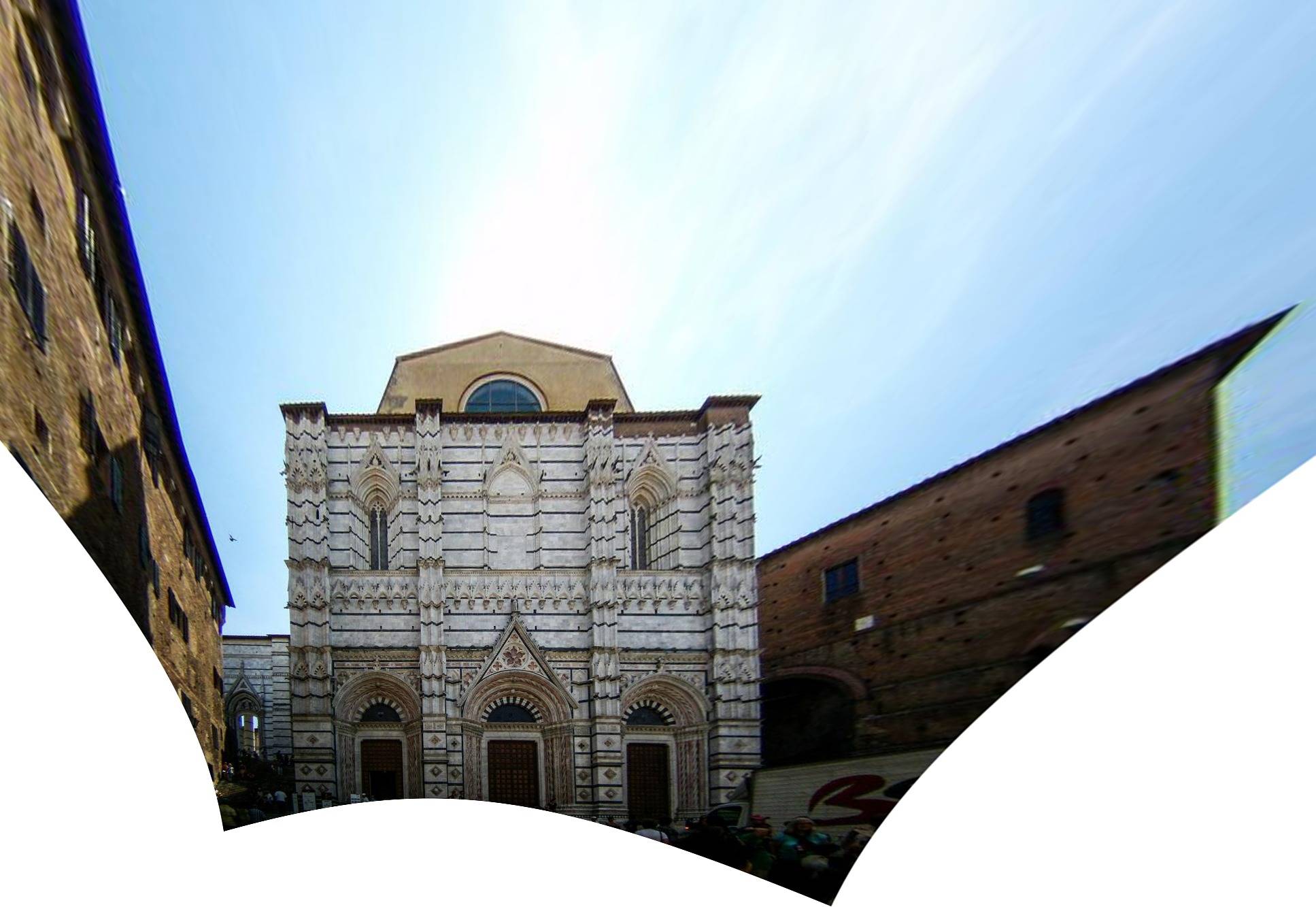
Radially-Distorted Conjugate Translations

Abstract

This paper introduces the first minimal solvers that jointly solve for affine-rectification and radial lens distortion from coplanar repeated patterns. Even with imagery from moderately distorted lenses, plane rectification using the pinhole camera model is inaccurate or invalid. The proposed solvers incorporate lens distortion into the camera model and extend accurate rectification to wide-angle imagery, which is now common from consumer cameras. The solvers are derived from constraints induced by the conjugate translations of an imaged scene plane, which are integrated with the division model for radial lens distortion. The hidden-variable trick with ideal saturation is used to reformulate the constraints so that the solvers generated by the Gröbner-basis method are stable, small and fast.

Rectification and lens distortion are recovered from either one conjugately translated affine-covariant feature or two independently translated similarity-covariant features. The proposed solvers are used in a ransac-based estimator, which gives accurate rectifications after few iterations. The proposed solvers are evaluated against the state-of-the-art and demonstrate significantly better rectifications on noisy measurements. Qualitative results on diverse imagery demonstrate high-accuracy undistortions and rectifications. The source code is publicly available.

1 Introduction

Scene-plane rectification is used in many classic computer-vision tasks, including single-view 3D reconstruction, camera calibration, grouping coplanar symmetries, and image editing [26, 21, 15]. In particular, the affine rectification of a scene plane transforms the camera’s principal plane so that it is parallel to the scene plane. This restores the affine invariants of the imaged scene plane, which include parallelism of lines and translational symmetries [9, 21]. There is only an affine transformation between the affine-rectified imaged scene plane and its real-world counterpart. The removal of the effects of perspective imaging is helpful to understanding the geometry of the scene plane.

Wide-angle imagery that has significant lens distortion is common since consumer photography is now dominated by mobile-phone and GoPro-type cameras. High-accuracy rectification from wide-angle imagery is not possible with only pinhole camera models [11, 25]. Lens distortion can be estimated by performing a camera calibration apriori, but a fully automated method is desirable.

Figure 1: Input (top left) is a distorted view of a scene plane, and the outputs (top right, bottom) are the the undistorted and rectified scene plane. The method is fully automatic.

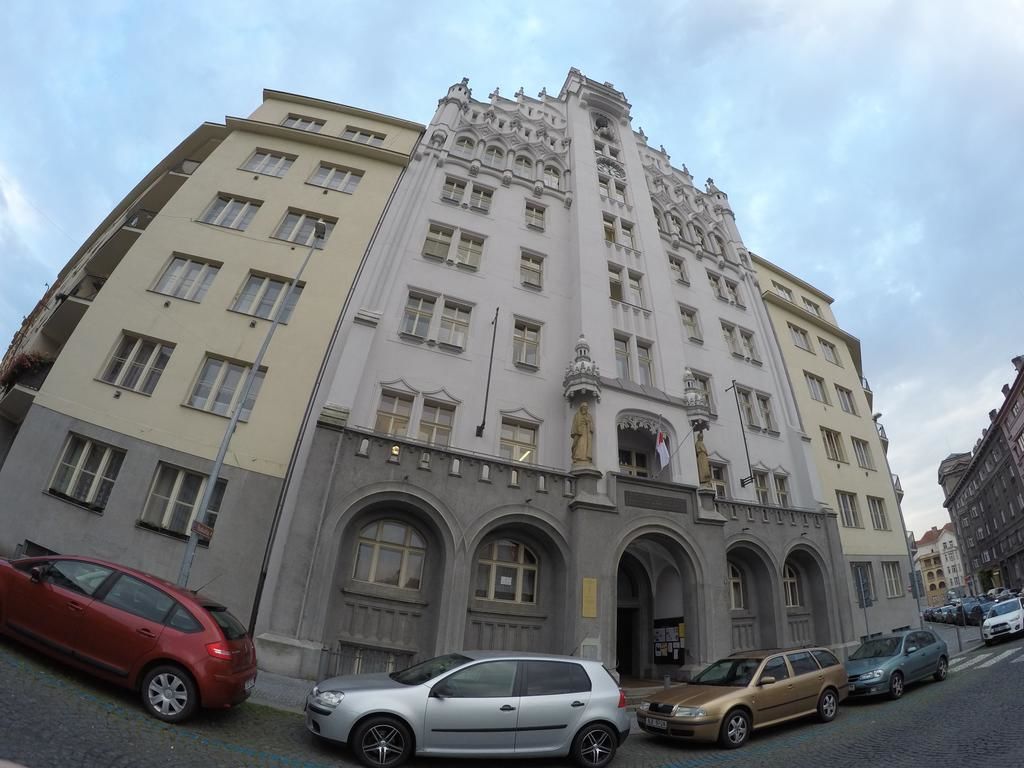
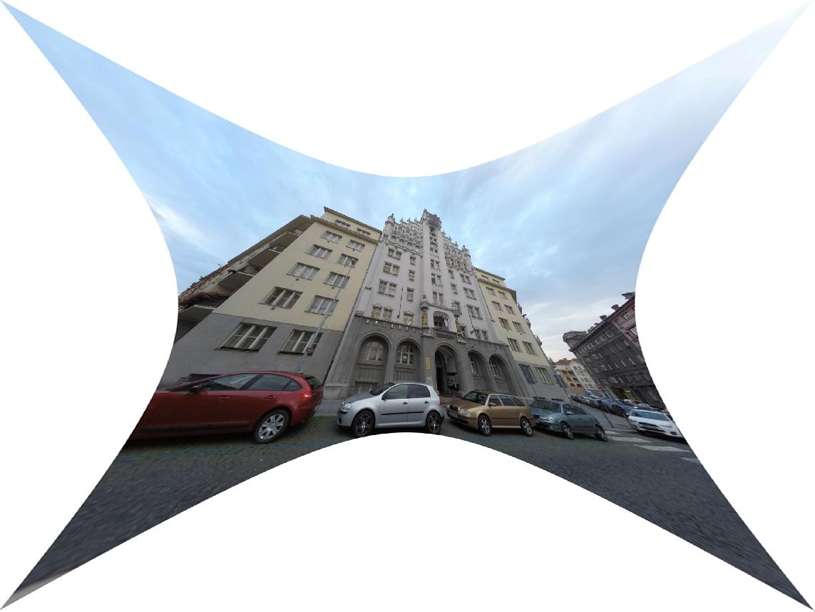
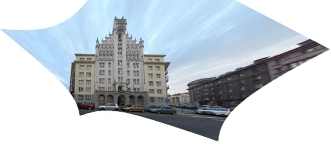
Several state-of-the-art planar-rectification methods assume a pinhole camera model, which ignores the effect of lens distortion [1, 4, 15, 27]. Pritts et al. [21] attempt to upgrade the pinhole camera model with radial lens distortion by giving an initial guess of the scene plane’s rectification that is consistent with a pinhole camera to a non-linear optimization that incorporates a lens-distortion model. However, even with relaxed thresholds, a robust estimator (i.e. ransac) will discard measurements that capture the most extreme effects of lens distortion, especially around the boundary of the image, since these measurements are not consistent with the pinhole-camera assumption. Thus, failing to account for lens distortion while labeling the measurements as outliers, as done during a ransac iteration, can give biased fits that underestimate the camera’s lens-distortion [11], which, in turn, reduces rectification accuracy.

narrow

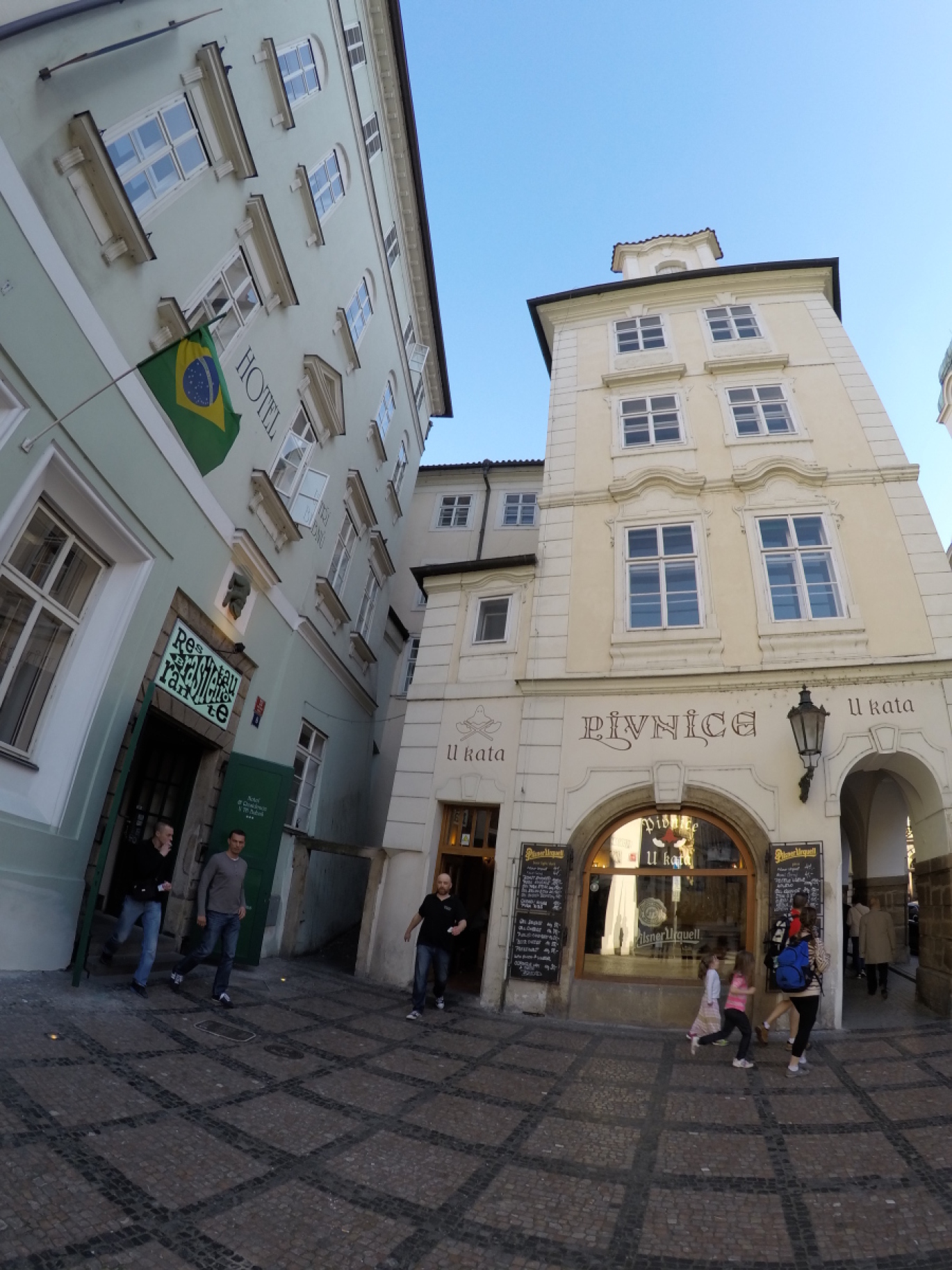
medium

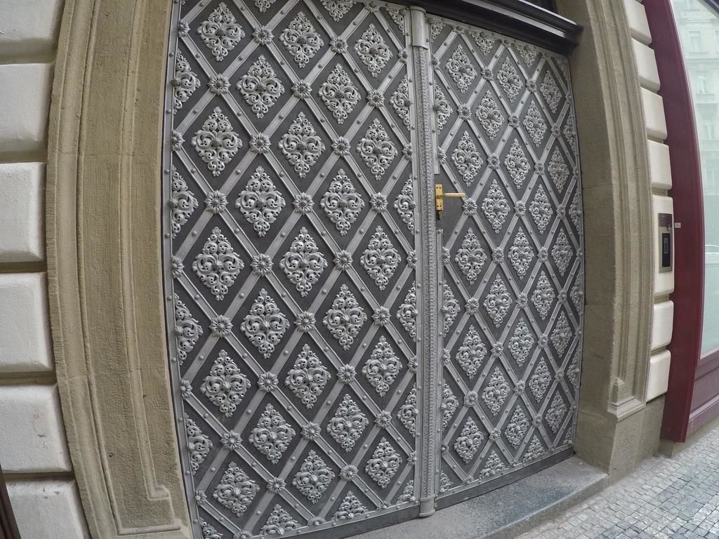
wide

Figure 2: GoPro Hero 4 imagery. (top row) Input images taken at different field-of-view settings. (bottom row) Rectified results.

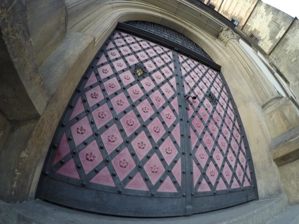
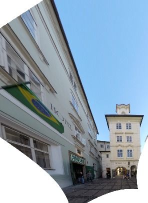
This paper introduces the first minimal solvers that jointly solve for the affine rectification of an imaged scene plane and a camera’s radial lens distortion. The solvers are derived from constraints induced by the conjugate translations of an imaged scene plane (see Sec. 2 for details), which are integrated with the division model of radial distortion [7]. Despite the simple formulation of the division model, it is accurate for even wide-angle lenses [7]. In addition, the solvers estimate the vanishing translation direction of the corresponded points used for input.

Two types of solvers are introduced: one-direction solvers, which require 3 coplanar point correspondences that translate in the same direction, and two-direction solvers, which require 4 coplanar point correspondences, 2 of which translate in one-direction and the remaining 2 in a different direction. Covariant feature detectors are used to extract the needed point correspondences [14, 16, 18, 19, 24]. The solvers are used in a ransac-based framework for robust rectification estimation. With one or two-correspondence sampling, an accurate undistortion and rectification is quickly recovered, even for difficult scenes.

Fitzgibbon used a one-parameter division model to develop a minimal solver for jointly estimating lens distortion with a fundamental matrix or homography [7]. Kukelova et al. [11] proposed an extension to [7] for homographies to model two-views from cameras with different radial lens distortions. These two-view solvers can jointly estimate lens distortion and conjugate translations, but are overparameterized for this task, which can result in inaccurate estimates as is shown by the synthetic experiments in Sec. 5. Wildenauer et al. [25] and Antunes et al. [2] are two methods that use constraints induced by imaged parallel lines to jointly solve for their vanishing point and the division model parameter, but but both require a multi-model estimation to recover scene-plane rectification (i.e. 2 consistent vanishing points).

The systems of polynomial equations induced from the constraints arising from joint estimation of conjugate translation with the division-model parameter are solved using an algebraic method based on Gröbner bases. Automated solver-generators using the Gröbner basis method [10, 12] were recently used to generate solvers for several problems in multi-view geometry [10, 13, 12, 11]. However, straightforward application of an automated solver-generator to the proposed problem resulted in unstable solvers (see Sec. 5). Therefore, we transformed the constraints to simplify the structure of the systems of polynomial equations, while explicitly accounting for the parasitic solutions that arose from the new formulation. The new formulation resulted in solvers with increased stability and speed.

The problem of rectification is closely coupled with the detection of coplanar repeats in a classic chicken-and-egg scenario: rectification is easy if the repeats are grouped, and repeats are more easily grouped if the affine invariants of the rectified plane are available [21]. Most methods tentatively group repeats from their local texture, which is verified later by a hypothesized rectification. Methods using this approach include Schaffalitzky et al. [23], which, similar to the solvers proposed in this paper, uses constraints induced by conjugate translations to recover the scene-plane’s vanishing line, and Chum et al. [4], which uses the constraint that coplanar repeats are equiareal in the scene-plane’s affine-rectified image. None of these methods account for lens distortion, and do not perform well on imagery with significant lens distortion (see Sec. 6).

2 Problem Formulation

Assume that the scene plane $\pi$ and a camera’s image plane $\pi^{\prime}$ are related point-wise by the homography $\mathtt{P}$, so that $\alpha_{i}\mathbf{x}^{\prime}_{i}=\mathtt{P}\mathbf{X}_{i}$, where $\alpha_{i}$ is a scalar, $\mathbf{X}_{i}\in\pi$ and $\mathbf{x}^{\prime}_{i}\in\pi^{\prime}$. Let $\mathbf{X}_{i}$ and $\mathbf{X}^{\prime}_{i}$ be two points on the scene plane $\pi$ such that $\mathbf{X}^{\prime}_{i}-\mathbf{X}_{i}=\mathbf{t}$. By encoding $\mathbf{t}$ in the homogeneous translation matrix $\mathtt{T}$, the points $\mathbf{X}_{i}$ and $\mathbf{X}^{\prime}_{i}$ as imaged by camera $\mathtt{P}$ can be expressed as

$$\alpha_{i}\mathbf{x}^{\prime}_{i}=\mathtt{P}\mathbf{X}^{\prime}_{i}=\mathtt{P}\mathtt{T}\mathbf{X}_{i}=\mathtt{P}\mathtt{T}\mathtt{P}^{{-1}}\mathbf{x}_{i}=\mathtt{H_{\mathbf{u}}}\mathbf{x}_{i},$$ (1)

where the homography $\mathtt{H}_{\mathbf{u}}=\mathtt{P}\mathtt{T}\mathtt{P}^{{-1}}$ is called a conjugate translation because of the form of its matrix decomposition and points $\mathbf{x}_{i}$ and $\mathbf{x}^{\prime}_{i}$ are in correspondence with respect to the conjugate translation $\mathtt{H}_{\mathbf{u}}$, which we denote $\mathbf{x}_{i}\leftrightarrow\mathbf{x}^{\prime}_{i}$ [9, 23]. Decomposing $\mathtt{H}_{\mathbf{u}}$ into its projective components gives

$$\alpha_{i}\mathbf{x}^{\prime}_{i} =\mathtt{H}_{\mathbf{u}}\mathbf{x}_{i}=\left[\mathtt{P}\mathtt{I}_{3}\mathtt{P}^{{-1}}+\mathtt{P}\begin{pmatrix}t_{x}\\ t_{y}\\ 1\end{pmatrix}\left[\mathtt{P}^{-{\!\top}}\begin{pmatrix}0\\ 0\\ 1\end{pmatrix}\right]^{{\!\top}}\right]\mathbf{x}_{i}$$

$$=[\mathtt{I}_{3}+s^{\mathbf{u}}_{i}\mathbf{u}\mathbf{l}^{{\!\top}}]\cdot\mathbf{x}_{i}$$ (2)

where $\mathtt{I}_{3}$ is the $3\times 3$ identity matrix, and

• line $\mathbf{l}$ is the imaged scene plane’s vanishing line,

• point $\mathbf{u}$ is the vanishing direction of translation, which must meet the vanishing line $\mathbf{l}$, i.e., $\mathbf{l}^{{\!\top}}\mathbf{u}=0$,

• and scalar $s^{\mathbf{u}}_{i}$ is the magnitude of translation in the direction $\mathbf{u}$ for the point correspondence $\mathbf{\tilde{x}}_{i}\leftrightarrow\mathbf{\tilde{x}}^{\prime}_{i}$ [23].

Note that (2) holds only for points projected by a pinhole camera viewing a scene plane, which is parameterized by the homography $\mathtt{P}$ as defined above. For every real camera, some amount of radial distortion is always present, so for (2) to hold, the measured image points $\mathbf{\tilde{x}}_{i}$ and $\mathbf{\tilde{x}}^{\prime}_{i}$ must first be undistorted. We use the one-parameter division model to parameterize the radial lens distortion [7], which has the form

$$f(\mathbf{\mathbf{\tilde{x}}_{i}},\lambda)=\begin{pmatrix}\tilde{x}_{i},&\tilde{y}_{i},&1+\lambda(\tilde{x}_{i}^{2}+\tilde{y}_{i}^{2})\end{pmatrix}^{{\!\top}},$$ (3)

where the distortion center is given; i.e., $\tilde{x}_{i},\tilde{y}_{i}$ are the center-subtracted measurements from a feature detector.

In this work we incorporate constraints induced by a conjugate translation as derived in (2) with the division model defined in (3) to accurately rectify imaged scene planes from lens-distorted cameras. Since the unknown division model parameter is exclusively encoded in the homogeneous coordinate, the relation for conjugate translations can be directly augmented to model lens distortion, namely,

$$\alpha_{i}f(\mathbf{\tilde{x}}^{\prime}_{i},\lambda)=\mathtt{H}_{\mathbf{u}}f(\mathbf{\tilde{x}}_{i},\lambda)=[\mathtt{I}_{3}+s^{\mathbf{u}}_{i}\mathbf{u}\mathbf{l}^{{\!\top}}]\cdot f(\mathbf{\tilde{x}}_{i},\lambda),$$ (4)

where $\alpha_{i}$ is some non-zero scalar, and $\mathbf{\tilde{x}}_{i}\leftrightarrow\mathbf{\tilde{x}}^{\prime}_{i}$ is a point correspondence.

3 Solvers

The model for radially-distorted conjugate translations in (4) defines the unknown geometric quantities: (i) division-model parameter $\lambda$, (ii) scene-plane vanishing line $\mathbf{l}=\begin{pmatrix}l_{1},&l_{2},&l_{3}\end{pmatrix}^{{\!\top}}$, (iii) vanishing translation direction $\mathbf{u}=\begin{pmatrix}u_{1},&u_{2},&u_{3}\end{pmatrix}^{{\!\top}}$ (see Sec. 3.2 for the two-direction extensions), (iv) scale of translation $s^{\mathbf{u}}_{i}$ for correspondence $\mathbf{\tilde{x}}_{i}\leftrightarrow\mathbf{\tilde{x}}^{\prime}_{i}$, (v) and the scalar parameter $\alpha_{i}$.

The solution for the vanishing line $\mathbf{l}$ is constrained to the affine subspace $l_{3}=1$ of the real-projective plane, which makes it unique. This inhomogeneous choice of $\mathbf{l}$ is unable to represent the pencil of lines that pass through the origin. If this degeneracy is encountered, then the scale of $\mathbf{l}$ is fixed by setting $l_{2}=1$ instead. Solver variants for both constraints are generated for all of the proposed solvers. In practice, this degeneracy is rarely encountered. If the $l_{3}=1$ solver variant suffers from bad numerical conditioning, then the $l_{2}=1$ variant can be activated and its solutions tested for consensus with the measurements (see Sec. 4). Without loss of generality the derivations below assume that $l_{3}=1$.

The vanishing direction $\mathbf{u}$ must meet the vanishing line $\mathbf{l}$, which defines a subspace of solutions for $\mathbf{u}$. The magnitude of $\mathbf{u}$ is set to the translation scale $s^{\mathbf{u}}_{1}$ of the first correspondence, which defines a unique solution

$$\mathbf{l}^{{\!\top}}\mathbf{u}=l_{1}u_{1}+l_{2}u_{2}+u_{3}=0\quad\wedge\quad\|\mathbf{u}\|=s^{\mathbf{u}}_{1}.$$ (5)

The relative scale of translation $\bar{s}^{\mathbf{u}}_{i}$ for each correspondence $\mathbf{\tilde{x}}_{i}\leftrightarrow\mathbf{\tilde{x}}^{\prime}_{i}$ with respect to the magnitude of $\|\mathbf{u}\|$ is defined so that $\bar{s}^{\mathbf{u}}_{i}={s^{\mathbf{u}}_{i}}/{\|\mathbf{u}\|}$. Note that $\bar{s}^{\mathbf{u}}_{1}=1$.

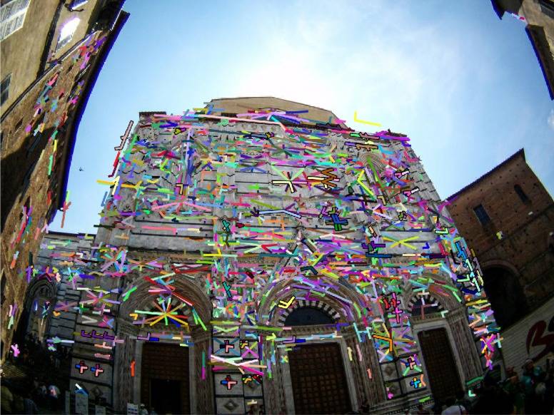
In this paper we propose four different minimal solvers for different variants of the problem of radially-distorted conjugate translations based on different translation directions and relative scales $\bar{s}^{\mathbf{u}}_{i}$. These variants are motivated by the types of covariant feature detectors used to extract point correspondences [14, 16, 18, 19, 24]. Each affine-covariant feature defines an affine frame, i.e. an ordered triplet of points. Thus, 1 affine-frame correspondence provides the 3 point correspondences that translate in the same direction with the same scale. This is sufficient input for the one-directional solvers. A visualization of the features is provided in Fig. C.4 of the supplemental material. In the case of similarity-covariant features, such as DoG [14], only a similarity frame can be constructed. A correspondence of similarity frames gives 2 point correspondences that translate jointly. Two correspondences of similarity-covariant features of different direction of the translation provide sufficient constraints for the two directional solvers.

Two one-direction solvers are proposed, which require 3 (2.5) coplanar point correspondences that translate in the same direction. The “3-point” solver $\mathtt{H}3\mathbf{l}\mathbf{u}s_{\mathbf{u}}\lambda$ assumes that two of the point correspondences have the same scale of translation (i.e. $\bar{s}^{\mathbf{u}}_{1}=\bar{s}^{\mathbf{u}}_{2}=1$), and the third point correspondence has an unknown relative scale of the translation $\bar{s}^{\mathbf{u}}_{3}$. The “2.5-point” solver $\mathtt{H}2.5\mathbf{l}\mathbf{u}\lambda$ assumes that all 3 point correspondences have the same relative scales of translation, i.e. $\bar{s}^{\mathbf{u}}_{1}=\bar{s}^{\mathbf{u}}_{2}=\bar{s}^{\mathbf{u}}_{3}=1$.

In addition, two two-direction solvers are proposed, which require 4 (3.5) coplanar point correspondences, 2 of which translate in one-direction $\mathbf{u}$ and the remaining 2 in a different direction $\mathbf{v}$. Here the “4-point” solver $\mathtt{H}4\mathbf{l}\mathbf{u}\mathbf{v}s_{\mathbf{v}}\lambda$ assumes that the first two point correspondences translate in the direction $\mathbf{u}$ with the same relative scale of translation, i.e., $\bar{s}^{\mathbf{u}}_{1}=\bar{s}^{\mathbf{u}}_{2}=1$. The remaining two point correspondence translate in the direction $\mathbf{v}$ with arbitrary translation magnitudes, i.e., the relative scales of translations of these two correspondences with respect to $\|\mathbf{v}\|=s^{\mathbf{v}}_{3}$ are $\bar{s}^{\mathbf{v}}_{3}=1$ and an unknown relative scale $\bar{s}^{\mathbf{u}}_{4}$.

The “3.5-point” $\mathtt{H}3.5\mathbf{l}\mathbf{u}\mathbf{v}\lambda$ solver assumes that the relative scales $\bar{s}^{\mathbf{u}}_{1}=\bar{s}^{\mathbf{u}}_{2}=1$ with respect to $\|\mathbf{u}\|=s^{\mathbf{u}}_{1}$ and $\bar{s}^{\mathbf{v}}_{3}=\bar{s}^{\mathbf{v}}_{4}=1$ with respect to $\|\mathbf{v}\|=s^{\mathbf{v}}_{3}$.

In all proposed solvers the scalar values $\alpha_{i}$ are eliminated from (4). This is done by multiplying (4) by the skew-symmetric matrix $[f(\mathbf{\tilde{x}}^{\prime}_{i},\lambda)]_{\times}$. The fact that the join of a point $\mathbf{x}_{i}$ with itself $[\mathbf{x}_{i}]_{\times}\mathbf{x}_{i}$ is $\mathbf{0}$ gives,

$$\begin{bmatrix}0&-\tilde{w}^{\prime}_{i}&\tilde{y}^{\prime}_{i}\\ \tilde{w}^{\prime}_{i}&0&-\tilde{x}^{\prime}_{i}\\ -\tilde{y}^{\prime}_{i}&\tilde{x}^{\prime}_{i}&0\end{bmatrix}$$

$$\times\begin{bmatrix}1+\bar{s}^{\mathbf{u}}_{i}u_{1}l_{1}&\bar{s}^{\mathbf{u}}_{i}u_{1}l_{2}&\bar{s}^{\mathbf{u}}_{i}u_{1}\\ \bar{s}^{\mathbf{u}}_{i}u_{2}l_{1}&1+\bar{s}^{\mathbf{u}}_{i}u_{2}l_{2}&\bar{s}^{\mathbf{u}}_{i}u_{2}\\ \bar{s}^{\mathbf{u}}_{i}u_{3}l_{1}&\bar{s}^{\mathbf{u}}_{i}u_{3}l_{2}&1+\bar{s}^{\mathbf{u}}_{i}u_{3}\end{bmatrix}\begin{pmatrix}\tilde{x}_{i}\\ \tilde{y}_{i}\\ \tilde{w}_{i}\end{pmatrix}=\mathbf{0},$$ (6)

where $\tilde{w}_{i}=1+\lambda(\tilde{x}^{2}_{i}+\tilde{y}^{2}_{i})$ and $\tilde{w}^{\prime}_{i}=1+\lambda(\tilde{x}^{\prime 2}_{i}+\tilde{y}^{\prime 2}_{i})$. The matrix equation in (6) contains three polynomial equations from which only two are linearly independent, since the skew-symmetric matrix $[f(\mathbf{\tilde{x}}^{\prime}_{i},\lambda)]_{\times}$ is rank two.

To solve the systems of polynomial equations resulting from the presented problems, we use the Gröbner basis method [6]. To generate efficient solvers we used the automatic generator of Gröbner basis solvers proposed in [10, 12]. However, for our problems the coefficients of the input equations are not fully independent. This means that using the default settings for the automatic generator [10, 12] that initialize the coefficients of equations by random values from $\mathbb{Z}_{p}$ does not lead to correct solvers. To obtain working Gröbner basis solvers, one has to create correct problems instances with values from $\mathbb{Z}_{p}$ for the automatic generator initialization.

The straightforward application of the automatic generator [10, 12] to the needed constraints with correct coefficients from $\mathbb{Z}_{p}$ resulted in large templates and unstable solvers, especially for the two-direction problems. The Gröbner basis solvers generated for the original constraints have template matrices with sizes $80\times 84$, $74\times 76$, $348\times 354$, and $730\times 734$ for the $\mathtt{H}2.5\mathbf{l}\mathbf{u}\lambda$, $\mathtt{H}3\mathbf{l}\mathbf{u}s_{\mathbf{u}}\lambda$, $\mathtt{H}3.5\mathbf{l}\mathbf{u}\mathbf{v}\lambda$ and $\mathtt{H}4\mathbf{l}\mathbf{u}\mathbf{v}s_{\mathbf{v}}\lambda$ problems, respectively. Therefore, we use the hidden-variable trick [6] to eliminate the vanishing translation directions together with ideal saturation [13] to eliminate parasitic solutions. The reformulated constraints are simpler systems in only 3 or 4 unknowns, and the solvers generated by the Gröbner basis method are smaller and more stable. The reduced eliminiation template sizes are also summarized in Sec. B of the supplemental material. Next, we describe the solvers based on the hidden-variable trick in more detail.

	$\mathtt{H}2\mathbf{l}\mathbf{u}$	$\mathtt{H}2.5\mathbf{l}\mathbf{u}\lambda$	$\mathtt{H}3\mathbf{l}\mathbf{u}s_{\mathbf{u}}\lambda$	$\mathtt{H}3.5\mathbf{l}\mathbf{u}\mathbf{v}\lambda$	$\mathtt{H}4\mathbf{l}\mathbf{u}\mathbf{v}s_{\mathbf{v}}\lambda$	$\mathtt{H}4\mathbf{l}\gamma$	$\mathtt{H}5\lambda$	$\mathtt{H}5\lambda_{1}\lambda_{2}$
Reference	[23]					[4]	[7]	[10]
Distortion		✓	✓	✓	✓		✓	✓
$\mathtt{H}_{\infty}$	✓	✓	✓	✓	✓	✓
# points	2	2.5	3	3.5	4	4	5	5
# solutions	1	4	2	6	4	1	18	5

Table 1: Proposed solvers (grey) vs. state-of-the-art.

3.1 One-Direction Solvers

For the “3-point” one-direction $\mathtt{H}3\mathbf{l}\mathbf{u}s_{\mathbf{u}}\lambda$ solver we have $\bar{s}^{\mathbf{u}}_{1}=\bar{s}^{\mathbf{u}}_{2}=1$. Therefore the constraints (6) result in two pairs of linearly independent equations without the scale parameter $\bar{s}^{\mathbf{u}}_{i}$ for $i=1,2$, and two linearly independent equations with an unknown relative scale $\bar{s}^{\mathbf{u}}_{3}$ for the third point correspondence, i.e.,  $i=3$. Additionally, we have the orthogonality constraint in (5). All together we have seven equations in seven unknowns ($l_{1},l_{2},u_{1},u_{2},u_{3},\bar{s}^{\mathbf{u}}_{3},\lambda$).

Note, that these equations are linear with respect to the vanishing translation direction $\mathbf{u}$. Therefore, we can rewrite the seven equations as

$$\mathtt{M}(l_{1},l_{2},\bar{s}^{\mathbf{u}}_{3},\lambda)\begin{pmatrix}u_{1}\\ u_{2}\\ u_{3}\\ 1\end{pmatrix}=\mathbf{0}$$ (7)

where $\mathtt{M}(l_{1},l_{2},\bar{s}^{\mathbf{u}}_{3},\lambda)$ is a $7\times 4$ matrix which elements are polynomials in $(l_{1},l_{2},\bar{s}^{\mathbf{u}}_{3},\lambda)$.

Since $\mathtt{M}(l_{1},l_{2},\bar{s}^{\mathbf{u}}_{3},\lambda)$ has a null vector, it must be rank deficient. Therefore, all the $4\times 4$ sub-determinants of $\mathtt{M}(l_{1},l_{2},\bar{s}^{\mathbf{u}}_{3},\lambda)$ must equal zero. This results in ${{7}\choose{4}}=35$ polynomial equations which only involve four unknowns.

Unfortunately, the formulation (7) introduces a one-dimensional family of false solutions. These are not present in the original system and corresponds to solutions where the first three columns of $\mathtt{M}$ become rank deficient. In this case there exist null vectors to $\mathtt{M}$ where the last element of the vector is zero, i.e. not on the same form as in (7).

These false solutions can be removed by saturating any of the $3\times 3$ sub-determinants from the first three columns of $\mathtt{M}$. The matrix $\mathtt{M}$ has the following form,

$$\small\mathtt{M}(l_{1},l_{2},\bar{s}^{\mathbf{u}}_{3},\lambda)=\begin{bmatrix}m_{11}&m_{12}&0&m_{14}\\ m_{21}&m_{22}&0&m_{24}\\ m_{31}&0&m_{33}&m_{34}\\ m_{41}&0&m_{43}&m_{44}\\ m_{51}&m_{52}&0&m_{54}\\ m_{61}&0&m_{63}&m_{64}\\ l_{1}&l_{2}&1&0\end{bmatrix}$$ (8)

where $m_{ij}$ are polynomials in $l_{1},l_{2},\bar{s}^{\mathbf{u}}_{3}$ and $\lambda$. We choose to saturate the $3\times 3$ sub-determinant corresponding to the first, second and last row since it reduces to only the top-left $2\times 2$ sub-determinant, i.e. $m_{11}m_{22}-m_{12}m_{21}$, which is only a quadratic polynomial in the unknowns. The other $3\times 3$ determinants are more complicated and leads to larger polynomial solvers. Using the saturation technique from Larsson et al. [13] we were able to create a polynomial solver for this saturated ideal. The size of the elimination template is $24\times 26$. Note that without using the hidden-variable trick the elimination template was $74\times 76$.

For the $\mathtt{H}2.5\mathbf{l}\mathbf{u}\lambda$ solver we can use the same hidden-variable trick. In this case $\bar{s}^{\mathbf{u}}_{1}=\bar{s}^{\mathbf{u}}_{2}=\bar{s}^{\mathbf{u}}_{3}=1$ and therefore the matrix $\mathtt{M}$ in (7) contains only three unknowns $l_{1},l_{2}$ and $\lambda$. The minimal number of point correspondences necessary to solve this problem is $2.5$. Therefore, for this problem we can drop one of the equations from (6), e.g., for $i=3$, and the matrix $\mathtt{M}$ in (7) has size $6\times 4$. In this case all $4\times 4$ sub-determinants of $\mathtt{M}$ result in 15 equations in 3 unknowns.

Similar to the 3 point case, this introduces a one-dimensional family of false solutions. The matrix $\mathtt{M}$ has a similar structure as in (8) and again it is sufficient to saturate top-left $2\times 2$ sub-determinant. For this formulation we were able to create a solver with template size $14\times 18$ (compared with $80\times 84$ without using hidden-variable trick)

3.2 Two-Direction Solvers

In the case of the two-direction $\mathtt{H}4\mathbf{l}\mathbf{u}\mathbf{v}s_{\mathbf{v}}\lambda$ solvers, the input equations for two vanishing translation directions $\mathbf{u}=\begin{pmatrix}u_{1},&u_{2},&u_{3}\end{pmatrix}^{{\!\top}}$ and $\mathbf{v}=\begin{pmatrix}v_{1},&v_{2},&v_{3}\end{pmatrix}^{{\!\top}}$ can be separated into two sets of equations, i.e., the equations containing $\mathbf{u}$ and the equations containing $\mathbf{v}$. Note that in this case we have two equations of the form (5), i.e., the equation for the direction $\mathbf{u}$ and the equation for the direction $\mathbf{v}$ and we have an unknown relative scale $\bar{s}^{\mathbf{v}}_{4}$. Therefore, the final system of 10 equations in 10 unknowns can be rewritten using two matrix equations as

$$\mathtt{M}_{1}(l_{1},l_{2},\lambda)\begin{pmatrix}u_{1}\\ u_{2}\\ u_{3}\\ 1\end{pmatrix}=\mathbf{0},\;\;\mathtt{M}_{2}(l_{1},l_{2},\bar{s}^{\mathbf{v}}_{4},\lambda)\begin{pmatrix}v_{1}\\ v_{2}\\ v_{3}\\ 1\end{pmatrix}=\mathbf{0}$$ (9)

where $\mathtt{M}_{1}$ and $\mathtt{M}_{2}$ are $5\times 4$ matrices where the elements are polynomials in $(l_{1},l_{2},\lambda)$ and $(l_{1},l_{2},\bar{s}^{\mathbf{v}}_{4},\lambda)$ respectively.

Again all $4\times 4$ sub-determinants of $\mathtt{M}_{1}$ and $\mathtt{M}_{2}$ must concurrently equal zero. This results in $5+5=10$ polynomial equations in four unknowns $(l_{1},l_{2},\bar{s}^{\mathbf{v}}_{4},\lambda)$. In this case, only 39 additional false solutions arise from the hidden-variable trick. The matrices $\mathtt{M}_{1}$ and $\mathtt{M}_{2}$ have a similar structure as in (8) and again it is sufficient to saturate the top-left $2\times 2$ sub-determinants to remove the extra solutions. By saturating these determinants we were able to create a solver with template size $76\times 80$ (previously $730\times 734$).

Finally, for the “3.5-point” two-direction $\mathtt{H}3.5\mathbf{l}\mathbf{u}\mathbf{v}\lambda$ solver $\bar{s}^{\mathbf{u}}_{1}=\bar{s}^{\mathbf{u}}_{2}=1$ and $\bar{s}^{\mathbf{v}}_{3}=\bar{s}^{\mathbf{v}}_{4}=1$ so we can drop one of the equations from the constraint (6), e.g., for $i=4$. Therefore, the matrix $\mathtt{M}_{2}$ from (9) has size $4\times 4$ and it contains only 3 unknowns $(l_{1},l_{2},\lambda)$. In this case all $4\times 4$ sub-determinants of $\mathtt{M}_{1}$ and $\mathtt{M}_{2}$ result in $5+1=6$ polynomial equations in three unknowns $(l_{1},l_{2},\lambda)$.

For this case we get 18 additional false solutions. Investigations in Macaulay2 [8] revealed that for this particular formulation it was sufficient to only saturate the top-left $2\times 2$ sub-determinant of $\mathtt{M}_{1}$ and the top-left element of $\mathtt{M}_{2}$. Saturating these we were able to create a polynomial solver with a template size of $54\times 60$ (previously $348\times 354$).

4 Robust Estimation

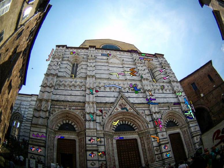
The solvers are used in a lo-ransac-based robust-estimation framework  [5]. Affine-covariant features are extracted from the image for input to the solvers. Affine-covariant features are highly repeatable on the same imaged scene texture with respect to significant changes of viewpoint and illumination [17]. Their proven robustness in the multi-view correspondence problem makes them good candidates for representing the local geometry of repeated textures. In particular, for the real-image experiments in Sec. 6, we use the Maximally-Stable Extremal Region and Hesssian-Affine detectors [16, 18]. The detections are parameterized as 3 distinct points, which define an affine coordinate frame in the image space [20]. These detections are visualized in Fig. C.4 of the supplemental material.

Affine frames are labeled as repeated texture based on the similarity of their appearance, which is given by the RootSIFT embedding of the image patch local to the affine frame [3, 14]. The RootSIFT descriptors are agglomeratively clustered, which establishes pair-wise tentative correspondences among the connected components linked by the clustering. Each appearance cluster has some proportion of its members that correspond to affine frames that give the geometry of imaged repeated scene content, which are the inliers of that appearance cluster. The remaining affine frames are the outliers.

lo-ransac samples pairs of affine frames from the appearance cluster, which are inputted to the proposed minimal solvers. Each pair of affine frames across all appearance clusters has an equi-probable chance of being drawn. The consensus with the minimal sample is measured by the number of pairs of affine frames within appearance groups that are consistent with the hypothesized model, normalized by the size of each respective group. A non-linear optimizer following [21] is used as the local optimization step of the lo-ransac estimator.

Figure 3: Stability study. Hidden-variable trick solvers are solid; standard solvers are dashed. The $\log_{10}$ transfer error is reported. The hidden-variable trick increases stability.

5 Synthetic Experiments

The proposed solvers are evaluated across several benchmarks on synthetic data against state-of-the-art solvers. Included in the benchmarks are two single-view solvers: $\mathtt{H}2\mathbf{l}\mathbf{u}$ [23], which also incorporates constraints from conjugate translations, and $\mathtt{H}4\mathbf{l}\gamma$ [4], which solves for rectification and change-of-scale, and also two full-homography and radial distortion solvers, $\mathtt{H}5\lambda$ [7] and $\mathtt{H}5\lambda_{1}\lambda_{2}$ [11], which we use for conjugate translation and lens-istortion estimation. The bench of state-of-the-art solvers is summarized in Table 1).

The benchmarks are evaluated for 1000 synthetic images of 3D scenes with known ground-truth parameters. A camera with a random but realistic focal length is randomly oriented and positioned with respect to a 10x10 square meter scene plane such that the plane is mostly in the camera’s field-of-view. Image resolution is set to 1000x1000 pixels. Conjugately translated affine frames are generated on the scene plane such that their scale with respect to the scene plane is realistic. This modeling choice reflects the use of affine-covariant feature detectors for real images. The conjugately translated features are distorted according to the division model, and, for the sensitivity experiments, isotropic white noise is added to the distorted affine frames at increasing levels. Performance is characterized by the relative error of the estimated distortion parameter and by the transfer and warp errors, which measure the accuracies of the estimated conjugate translation and rectification (see Sec. 5.1 - 5.4). The proposed solvers have an average solve time from 0.3 to 2 milliseconds over the 1000 synthetic scenes (see also Sec. B of the supplemental material).

5.1 Transfer Error

The geometric transfer error jointly measures the accuracy of an the estimated conjugate translation and lens distortion. The scene plane is tesselated by a 10x10 square grid of points $\{\,\mathbf{X}_{i}\}$. Let the translation on the scene plane induced by the noiseless pre-images of the point correspondences used to estimate $\hat{\mathtt{H}}_{\mathbf{u}}$ and $\hat{\lambda}$ be $\mathbf{t}$. Then the grid points are translated by $\mathbf{t}{}/\|\mathbf{t}\|$ to $\{\,\mathbf{X}_{i}^{\prime}\}$. The grid and its translation are imaged by the ground-truth lens-distorted camera parameterized by matrix $\mathtt{P}$ and division-model parameter $\lambda$. The imaged grid is given by $\mathbf{\tilde{x}}_{i}=f^{d}(\mathtt{P}\mathbf{X}_{i},\lambda)$ and the translated grid by $\mathbf{\tilde{x}}^{\prime}_{i}=f^{d}(\mathtt{P}\mathbf{X}_{i}^{\prime},\lambda)$, where $f^{d}$ is the the function that transforms from pinhole points to radially-distorted points. Then the geometric transfer error is defined as

$$\Delta_{i}^{\mathrm{xfer}}=d(f^{d}([\mathtt{I}_{3}+\frac{1}{\|\mathbf{t}\|}(\hat{\mathtt{H}}_{\mathbf{u}}-\mathtt{I}_{3})]f(\mathbf{\tilde{x}}_{i},\hat{\lambda}_{1}),\hat{\lambda}_{2}),\mathbf{\tilde{x}}^{\prime}_{i}),$$ (10)

where $d(\cdot,\cdot)$ is the Euclidean distance. All solvers except $\mathtt{H}5\lambda_{1}\lambda_{2}$ have the constraint that $\hat{\lambda}_{1}=\hat{\lambda}_{2}$ [11]. The root-mean-square of transfer errors $\Delta_{\mathrm{RMS}}^{\mathrm{xfer}}$ for correspondences $\{\,(\mathbf{\tilde{x}}_{i},\mathbf{\tilde{x}}^{\prime}_{i})\,\}$ is reported. For two-direction solvers, the transfer error in the second direction is included in $\Delta_{\mathrm{RMS}}^{\mathrm{xfer}}$. The transfer error is used in the stability study, where the solvers are tested over varying division model parameters and in the sensitivity study, where the solvers are tested over varying noise levels with fixed division model parameter. The solver $\mathtt{H}4l\gamma$ of [4] does not estimate conjugate translations, so it is not reported. For a derivation of (10) see Sec. A in the supplementary material.

5.2 Numerical Stability

The stability study measures the RMS transfer error of solvers (see Sec. 5.1) for noiseless affine-frame correspondences across realistic scene and camera configurations generated as described in the introduction to this section. The ground-truth parameter of the division model $\lambda$ is drawn uniformly at random from the interval $[-6,0]$. For a reference, the division parameter of $\lambda=-4$ is typical for wide field-of-view cameras like the GoPro where the image is normalized by ${1}\over{width+height}$. Fig. 3 reports the histogram of $\log_{10}$ RMS transfer errors. For all new solvers we evaluate a solver generated from constraints derived with (solid histogram) and without (dashed histogram) the hidden-variable trick. The hidden-variable trick significantly improves the stability of the proposed solvers. The increased stabilities of the hidden-variable solvers most likely result from the reduced size of the G-J elimination problems needed by these solvers. The hidden-variable solvers are used for the remainder of the experiments.

Figure 4: Comparison of the transfer error (left, see Sec. 5.1) and the relative radial distortion error (right) after 25 iterations of a simple ransac for different solvers over increasingly noisy measurements for 1000 scenes.

5.3 Noise Sensitivity

The proposed and state-of-the-art solvers solvers are tested with increasing levels of white noise added to the affine correspondences induced by the ground-truth conjugate translation and lens distortion parameter. The white noise is parameterized by the standard-deviation of a zero-mean isotropic Gaussian distribution, and the solvers are tested at noise levels of $\sigma\in\{0.1,0.5,1,2\}$. The ground truth division model parameter is set to $\lambda=-4$, which is typical for GoPro-type imagery. The solvers are wrapped in

Figure 5: Warp-error comparison (see Sec. 5.4) after 25 iterations of a simple ransac for different solvers over increasingly noisy measurements for 1000 scenes.

a simple RANSAC-loop, which minimizes the RMS transfer error $\Delta_{\mathrm{RMS}}^{\mathrm{xfer}}$ over 25 sampled affine-frame correspondences. Results are calculated from the estimate given by ransac and summarized for the 1000 generated scenes as boxplots. The interquartile range is contained within the extents of a box, and the median is the horizontal line dividing the box.

As shown in Fig. 4 the proposed solvers give the most accurate joint estimation of conjugate translation and division model parameter as measured by the RMS transfer error $\Delta_{\mathrm{RMS}}^{\mathrm{xfer}}$ and relative error of estimated divsion model parameter. As expected, the minimal parameterization of the radially-distorted conjugate translation solvers—$\mathtt{H}2.5\mathbf{l}\mathbf{u}\lambda,\mathtt{H}3\mathbf{l}\mathbf{u}s_{\mathbf{u}}\lambda,\mathtt{H}3.5\mathbf{l}\mathbf{u}\mathbf{v}\lambda,\mathtt{H}4\mathbf{l}\mathbf{u}\mathbf{v}s_{\mathbf{v}}\lambda$—show significantly less sensitivity to noise than the overparmeterized radially-distorted homography solvers $\mathtt{H}5\lambda$ and $\mathtt{H}5\lambda_{1}\lambda_{2}$ for both measures. The solver $\mathtt{H}2\mathbf{l}\mathbf{u}$ shows significant bias (see the transfer error boxplots in Fig. 4) since it does not model lens distortion.

5.4 Warp Error

Since the accuracy of scene-plane rectification is a primary concern, we also report the warp error for rectifying homographies proposed by Pritts et al. [22], which we augment with the division model for radial lens distortion. A rectifying homography $\mathtt{H}_{\infty}$ of an imaged scene plane is constructed from its vanishing line $\mathbf{l}$ (see [9]). A round trip between the image space and rectified space is made by undistorting and rectifying imaged coplanar points by the estimated lens distortion $\hat{\lambda}$ and rectifying homography $\mathtt{\hat{H}_{\infty}}$ and then re-warping and distorting the rectified points into the image by a synthetic camera constructed from the ground-truth lens distortion $\lambda$ and rectifying homography $\mathtt{H}_{\infty}$. Ideally, the synthetic camera constructed from the truth would project the undistorted and rectified points onto the original points.

Note that there is an affine ambiguity, denoted $\mathtt{A}$, between $\mathtt{\hat{H}_{\infty}}$ and $\mathtt{H}_{\infty}$, which is folded into the expression for the synthetic camera, namely $\mathtt{P}(\mathtt{A})=(\mathtt{A}\mathtt{H}_{\infty})^{{-1}}$, and estimated during computation of the warp error,

$$\Delta^{\mathrm{warp}}=\min_{\hat{\mathtt{A}}}\sum_{i}d^{2}(\mathbf{\tilde{x}}_{i},f^{d}(\mathtt{P}(\hat{\mathtt{A}})\mathtt{\hat{H}_{\infty}}f(\mathbf{\tilde{x}}_{i},\hat{\lambda})),\hat{\lambda}),$$ (11)

where $d(\cdot,\cdot)$ is the Euclidean distance, and $\{\mathbf{\tilde{x}}_{i}\}$ are the imaged grid points of the scene-plane tesselation as defined in Sec. 5.1. The root mean square warp error for $\{\,\mathbf{\tilde{x}}_{i}\,\}$ is reported and denoted as $\Delta^{\mathrm{warp}}_{\mathrm{RMS}}$. The vanishing line is not directly estimated by solvers $\mathtt{H}5\lambda$ of [7] and $\mathtt{H}5\lambda_{1}\lambda_{2}$ of [11], so they are not reported.

Original image

$\mathtt{H}2\mathbf{l}\mathbf{u}$ + LO; $11.2\%$ inliers

$\mathtt{H}2.5\mathbf{l}\mathbf{u}\lambda$+LO; $20.4\%$ inliers

$\mathtt{H}3.5\mathbf{l}\mathbf{u}\mathbf{v}\lambda$+LO; $20.2\%$ inliers

Figure 6: GoPro Hero 4 at the wide setting for different solvers. Results from lo-ransac (see Sec. 4) for $\mathtt{H}2\mathbf{l}\mathbf{u}$, which omits distortion, and the proposed solvers $\mathtt{H}2.5\mathbf{l}\mathbf{u}\lambda$ and $\mathtt{H}3.5\mathbf{l}\mathbf{u}\mathbf{v}\lambda$. The top row has rectifications after local optimization (LO); The bottom row has undistortions estimated from the best minimal sample. lo-ransac cannot recover from the poor initializations by $\mathtt{H}2\mathbf{l}\mathbf{u}$ (column 2). The proposed solvers in columns 3 and 4 give a correct rectification. The bottom left has a chessboard undistorted using the division parameter estimated from the building facade by $\mathtt{H}2.5\mathbf{l}\mathbf{u}\lambda$+LO.

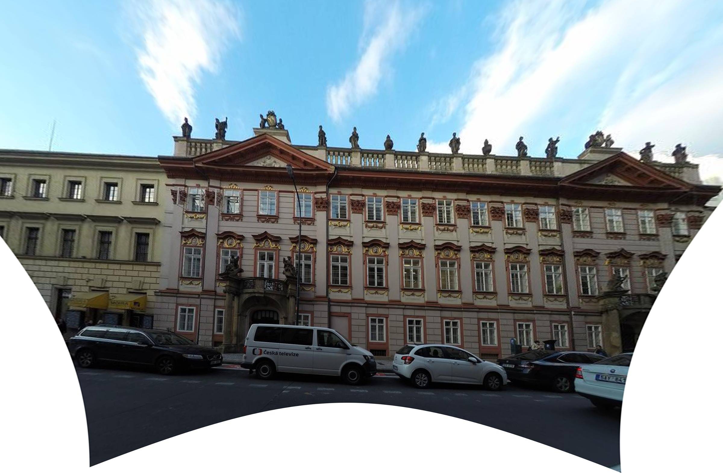
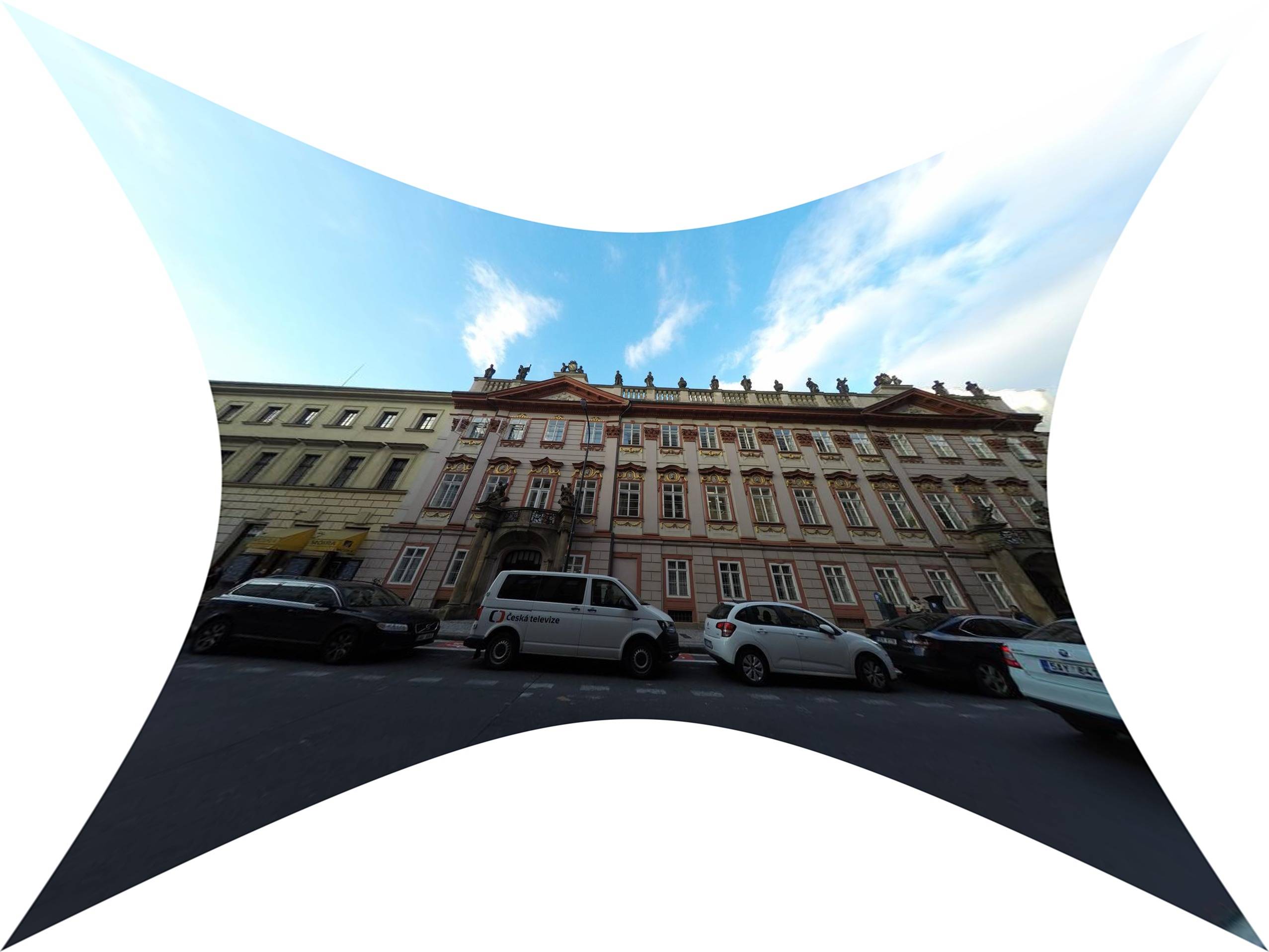
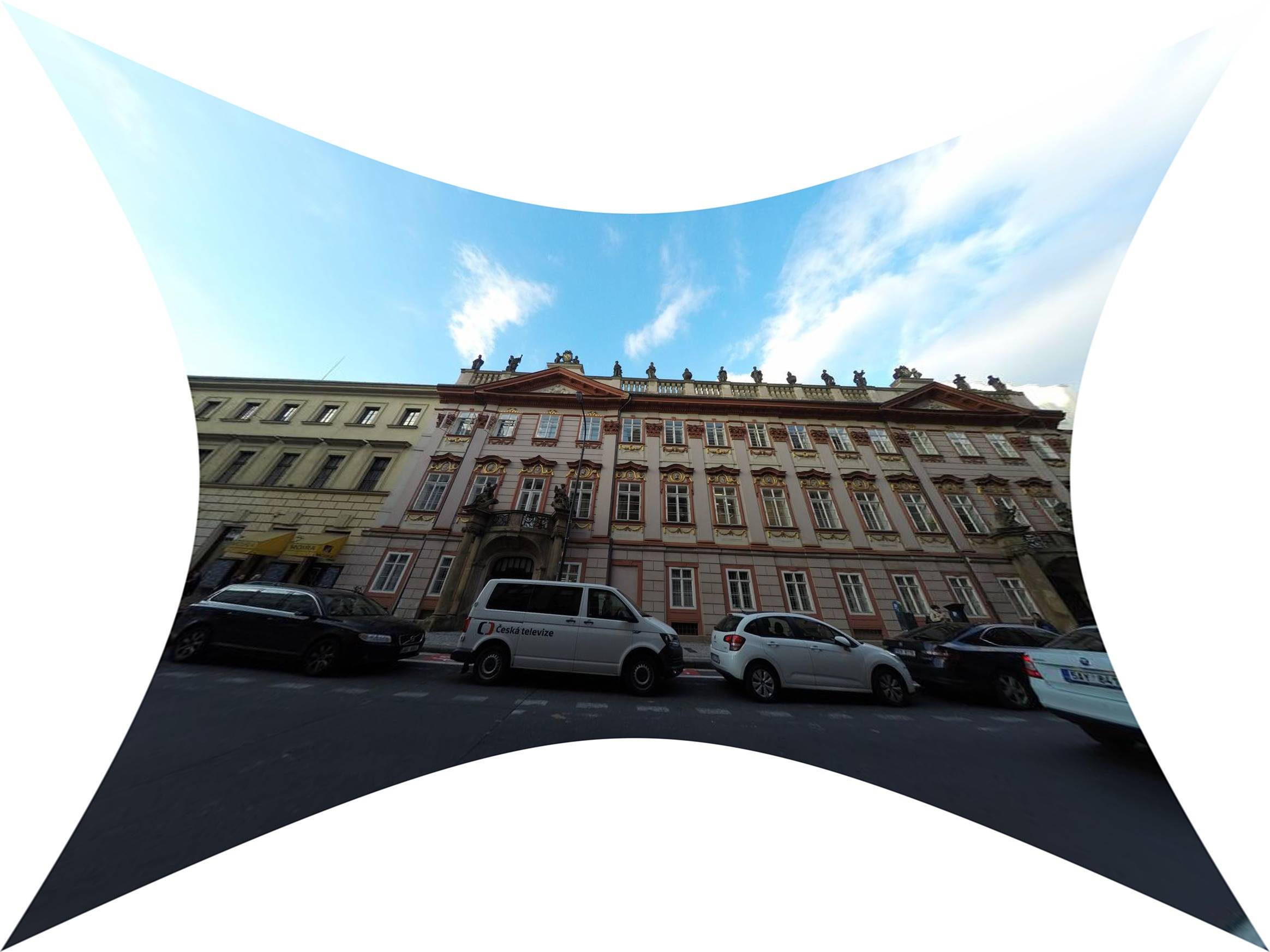
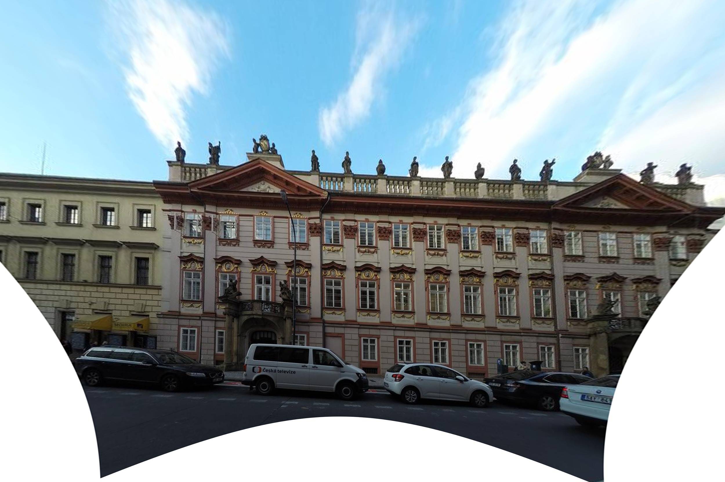
The proposed solvers—$\mathtt{H}2.5\mathbf{l}\mathbf{u}\lambda,\mathtt{H}3\mathbf{l}\mathbf{u}s_{\mathbf{u}}\lambda,\mathtt{H}3.5\mathbf{l}\mathbf{u}\mathbf{v}\lambda,$ $\mathtt{H}4\mathbf{l}\mathbf{u}\mathbf{v}s_{\mathbf{v}}\lambda$—estimate rectifications with less than 5 pixel RMS warp error $\Delta^{\mathrm{warp}}_{\mathrm{RMS}}$, even at the 2 pixel noise level, see Fig. 5. The need to model radial lens distortion is shown by the biased fits for the solvers $\mathtt{H}2\mathbf{l}\mathbf{u},\mathtt{H}4\gamma$.

6 Real Images

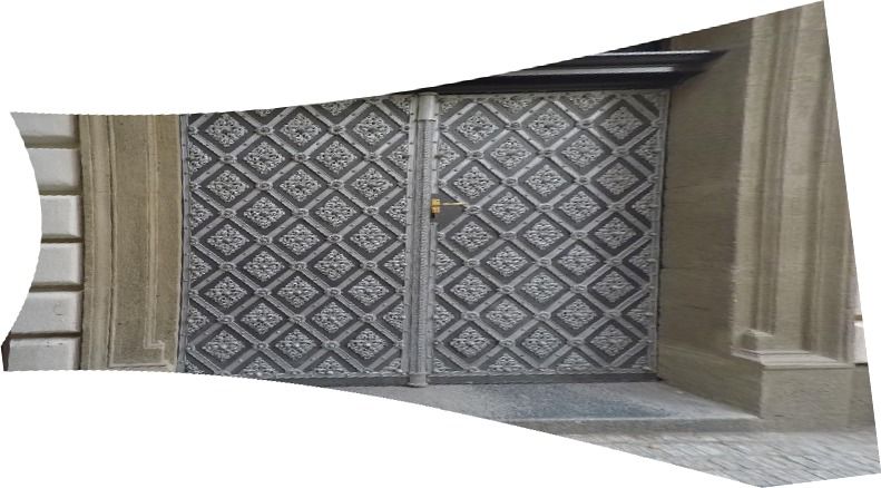
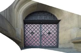
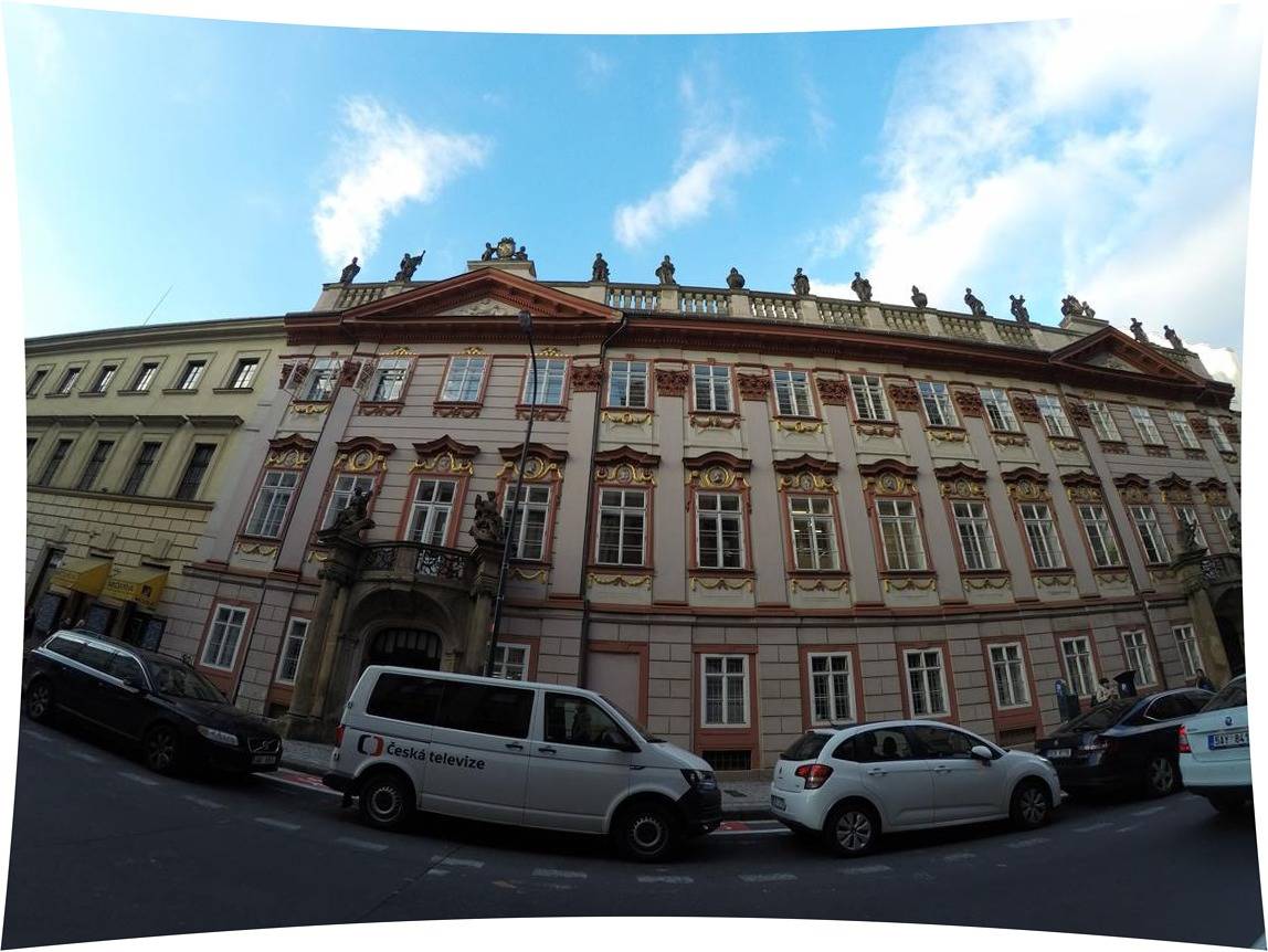
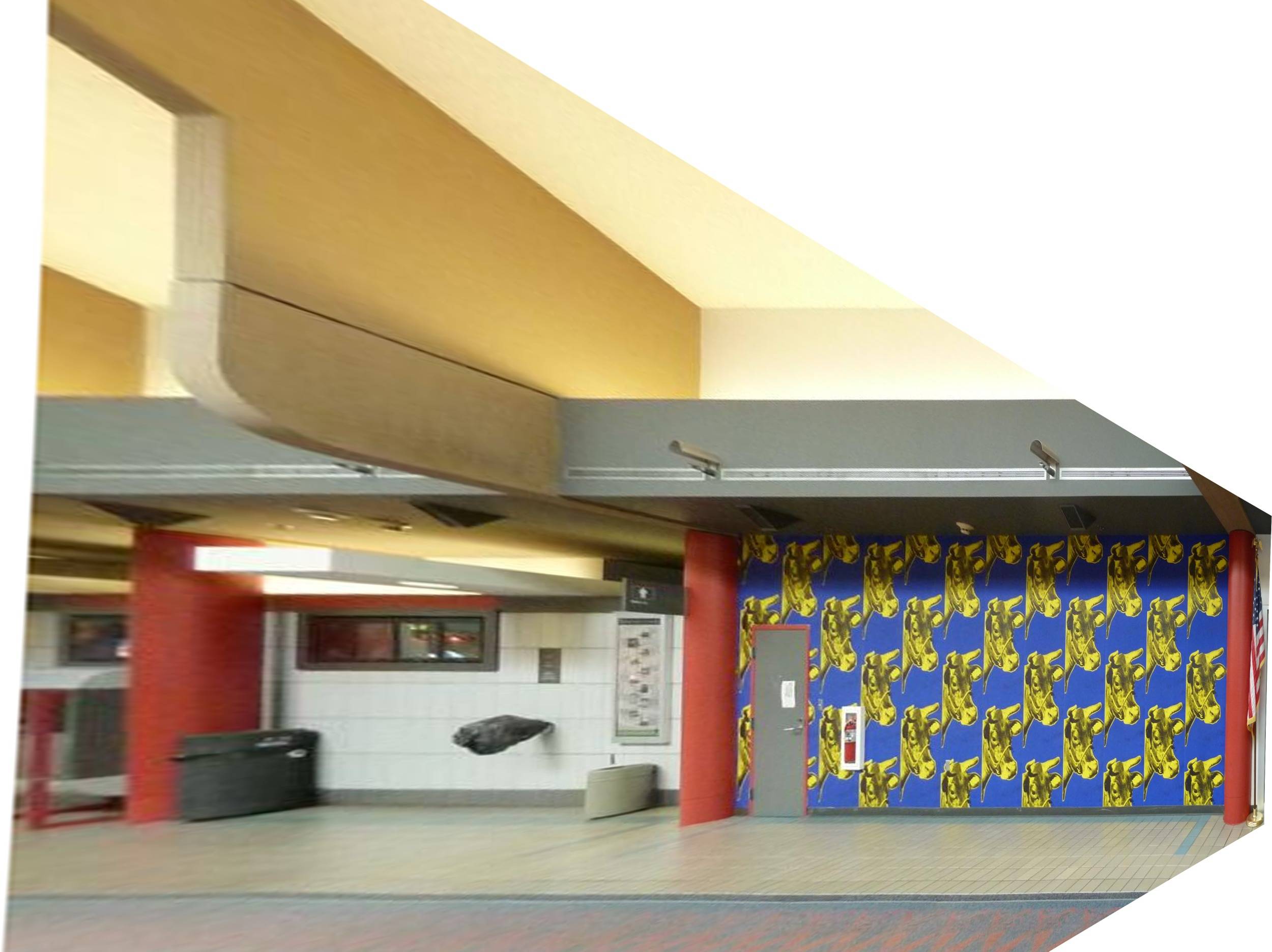
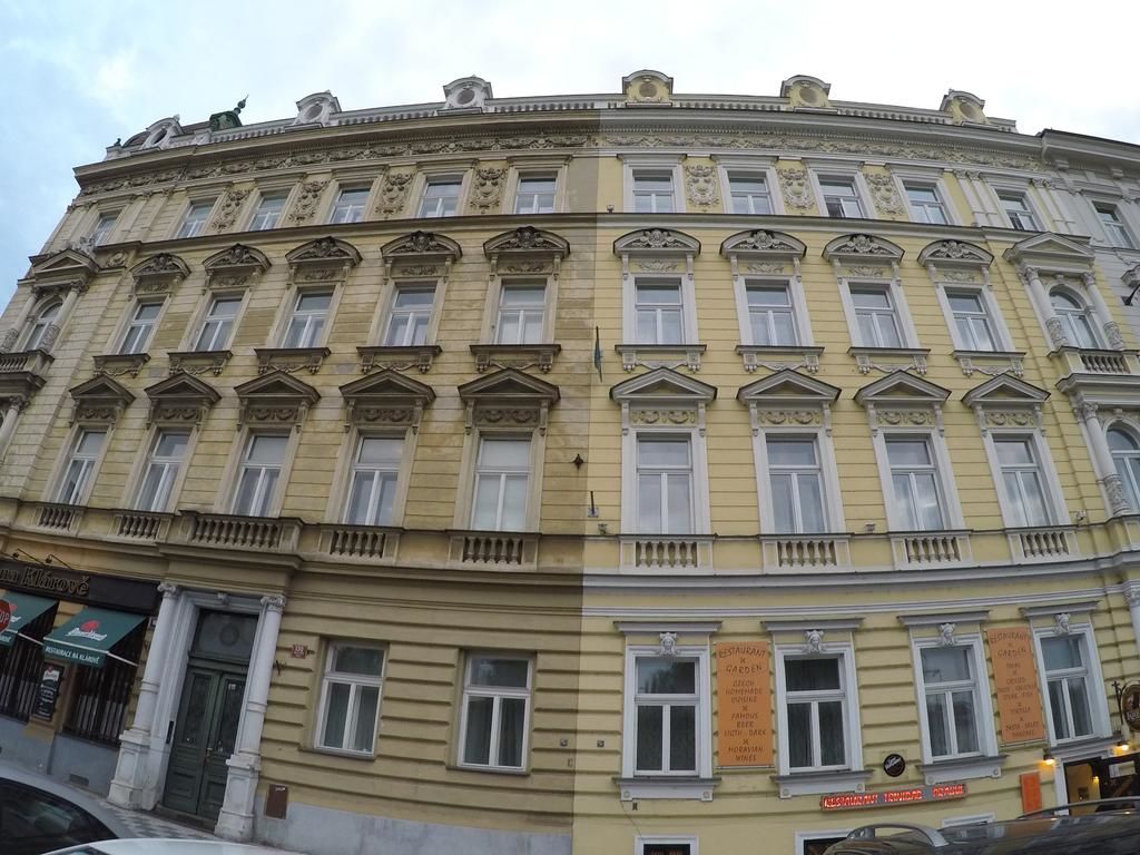
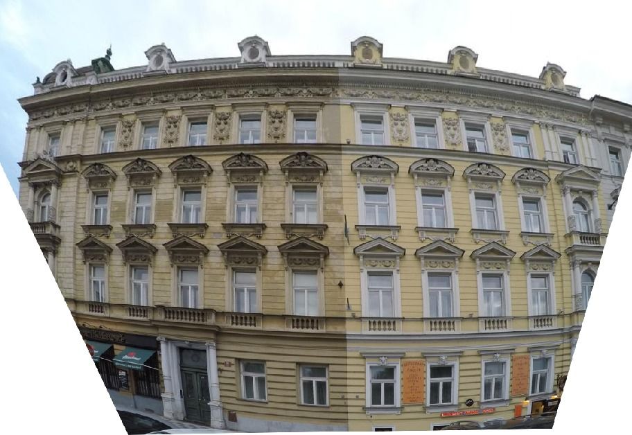
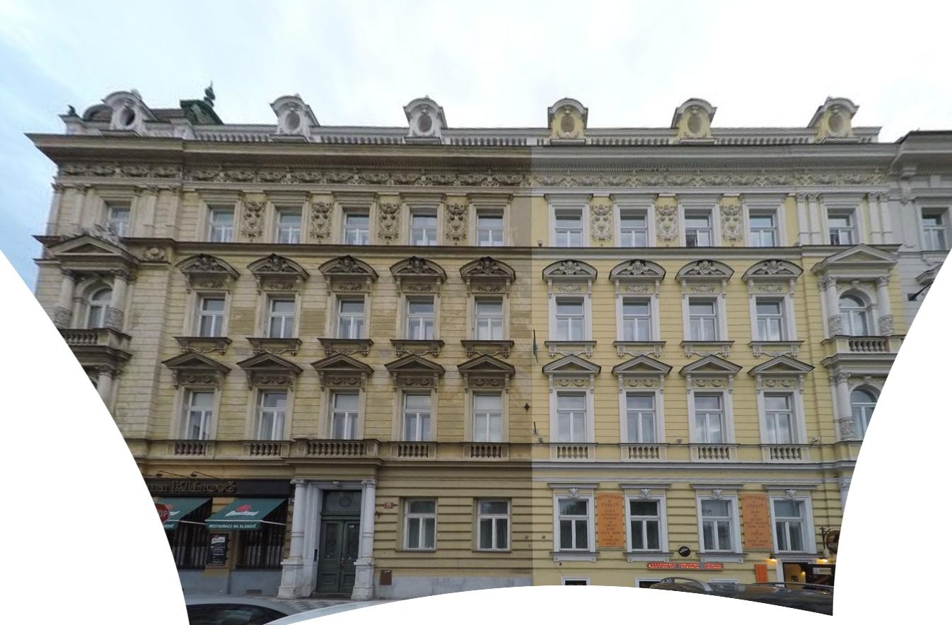
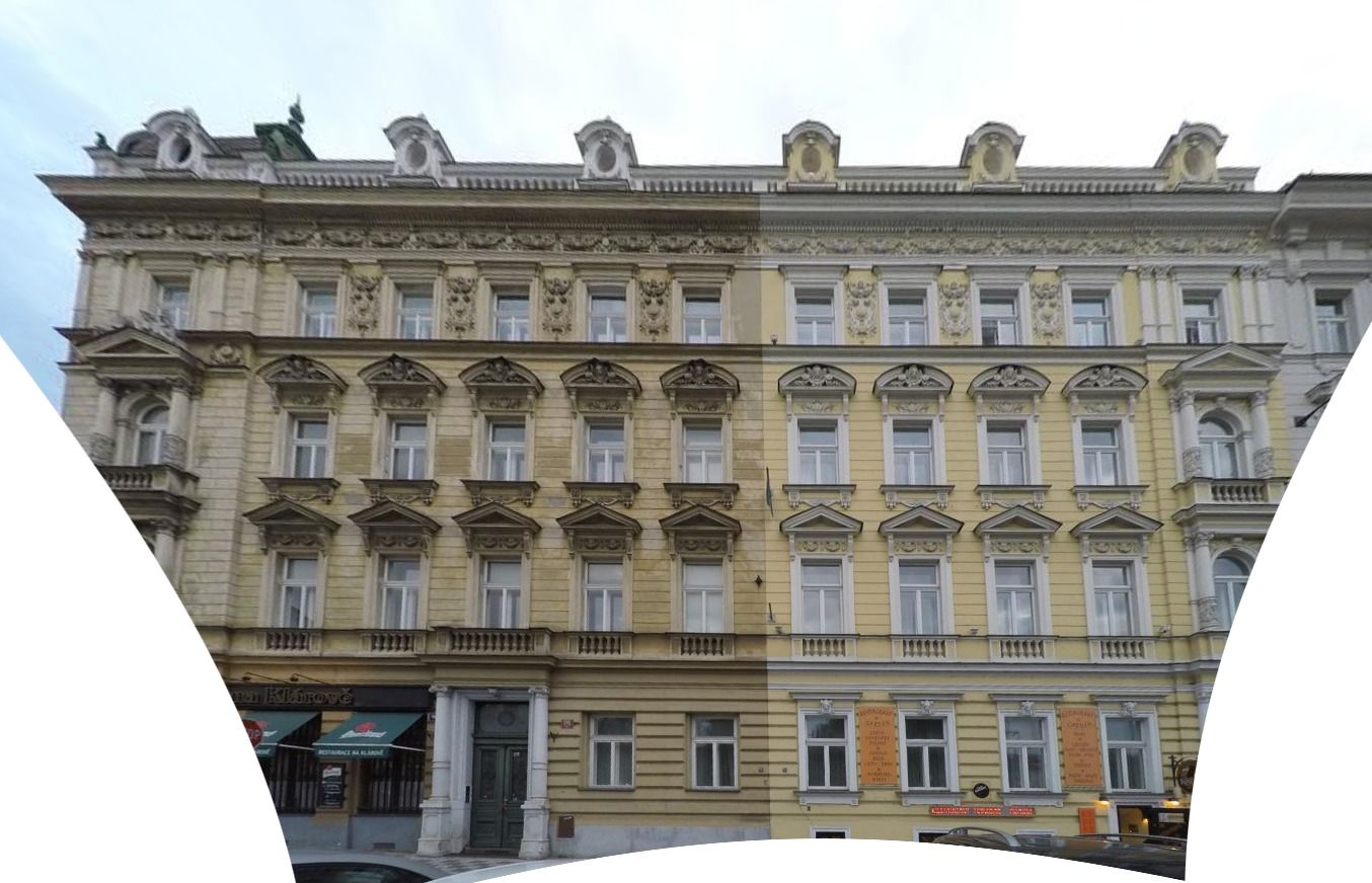
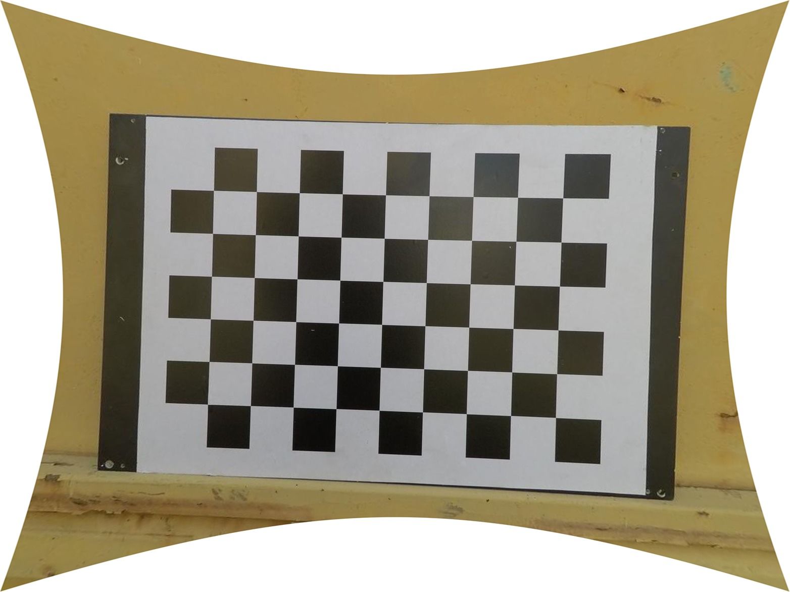
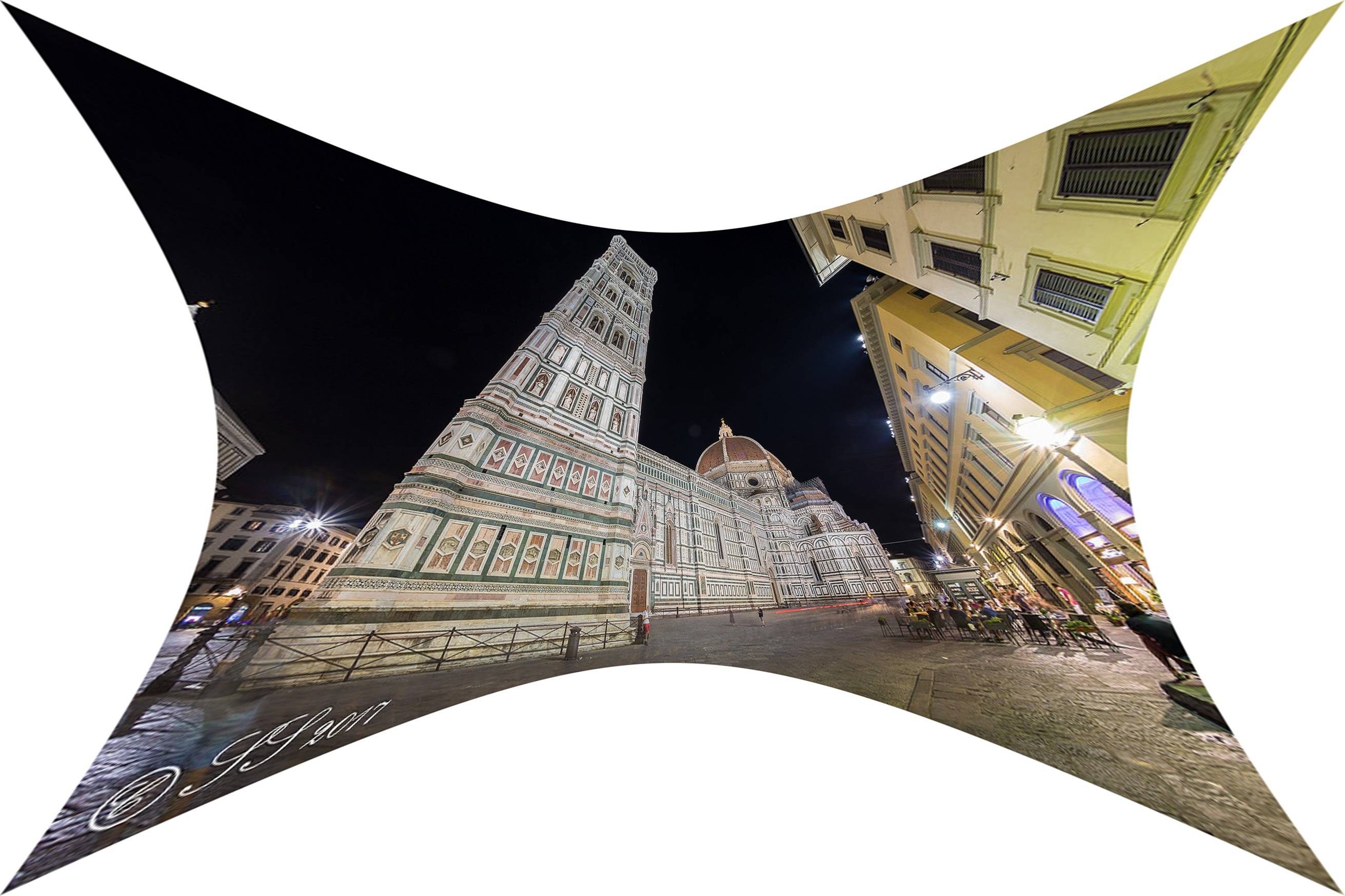
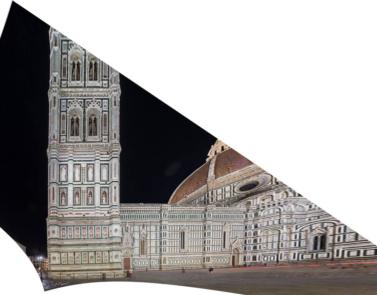
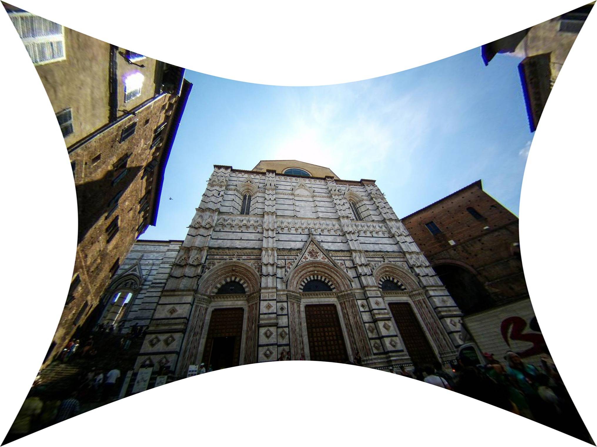
In the qualitative experiments on real images shown in Figs. 1 and  2, we tested the proposed solvers on GoPro4 Hero 4 images with increasing field-of-view settings, namely narrow, medium and wide, where a wider field-of-view setting generates more extreme radial distortion since the boundary of the lens is used. The proposed method generates high-quality rectifications at all the field-of-view settings. More real-image experiments, including results for cameras with radial distortions that are typical for mobile phone cameras and fisheye lenses (e.g., 8mm lens) can be found in Sec. C in the supplementary material.

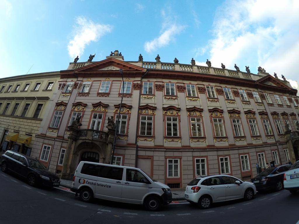
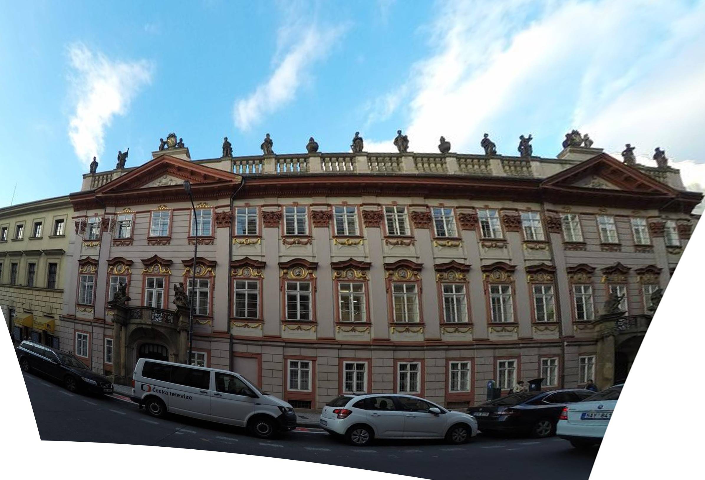
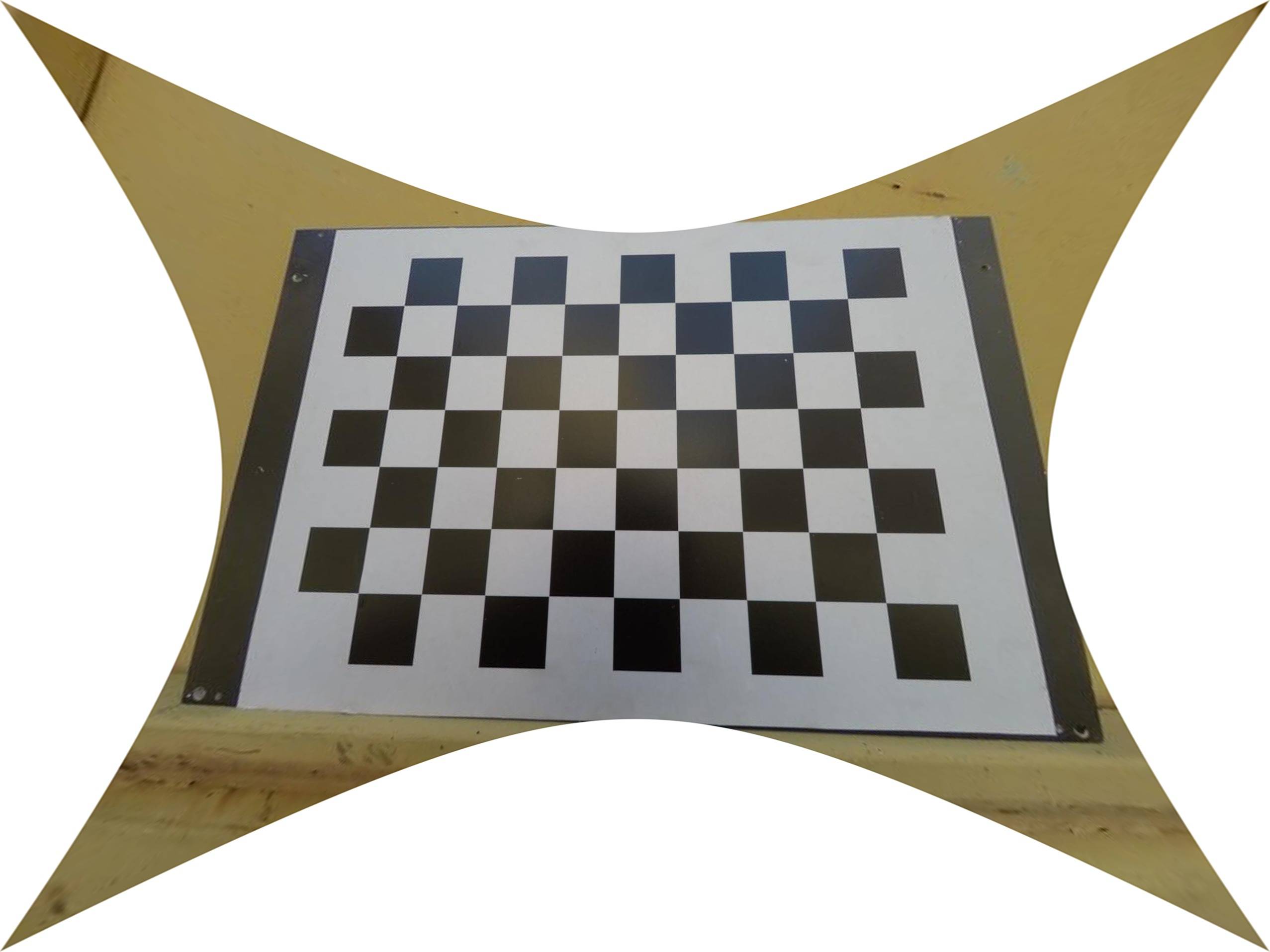
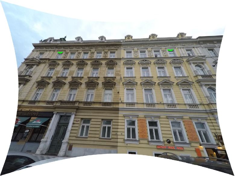
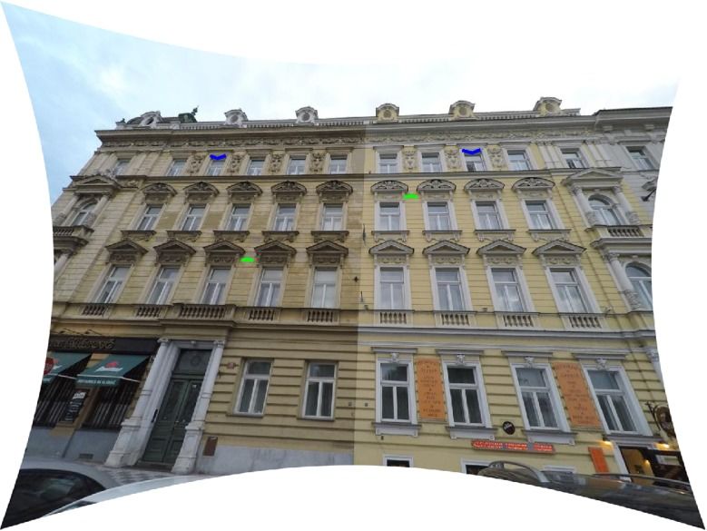
The experiment shown in Fig. 6 compares the performance of two of the proposed solvers, $\mathtt{H}2.5\mathbf{l}\mathbf{u}\lambda$ and $\mathtt{H}3.5\mathbf{l}\mathbf{u}\mathbf{v}\lambda$, to $\mathtt{H}2\mathbf{l}\mathbf{u}$ in a state-of-the-art local-optimization (LO) framework (see Sec. 4) on an GoPro Hero 4 image at the wide field-of-view setting. The two proposed solvers accurately estimate the division-model parameter (see the undistorted reference chessboard in Fig. 6) and the rectification, while the LO-variant using the $\mathtt{H}2\mathbf{l}\mathbf{u}$ solver is unable to recover the lens distortion parameter. See Fig. C.2 in the supplemental material for results on an image at the medium field-of-view setting.

7 Conclusions

This paper proposes the first minimal solvers that jointly solve for the affine rectification of an imaged scene plane and a camera’s radial lens distortion from coplanar repeated patterns. Rectification and radial lens distortion are recovered from only one conjugately translated affine-covariant feature or two independently translated similarity-covariant features. Synthetic experiments demonstrate the good stability and superior robustness to noise with respect to measures of rectification accuracy and lens-distortion estimation of the proposed solvers as compared to the state-of-the-art. However, the polynomial constraint equations that arise from conjugate translations distorted by the division model need to be transformed with the hidden-variable trick to generate stable solvers, though. Qualitative real-image experiments demonstrate high-quality rectifications for highly-distorted wide-angle lenses, which was not possible using the state-of-the-art. Future work could include conditionally sampling the measurements during robust estimation to take into account their size, relative distance from each other, or distance from the distortion center. We expect these factors have a big impact on rectification quality, but this study was beyond scope for this paper.

8 Acknowledgements

James Pritts was supported by the grants MSMT LL1303 ERC-CZ and SGS17/185/OHK3/3T/13, Zuzana Kukelova by the Czech Science Foundation Project GACR P103/12/G084, Viktor Larsson by the strategic research projects ELLIIT and eSSENCE, Swedish Foundation for Strategic Research project ”Semantic Mapping and Visual Navigation for Smart Robots” (grant no. RIT15-0038) and Wallenberg Autonomous Systems and Software Program (WASP), and Ondrej Chum by the grant MSMT LL1303 ERC-CZ.

Appendix A Transfer Error

The scene plane is tessellated by a 10x10 square grid of points, denoted $\{\,\mathbf{X}_{i}\,\}$, with a 1 meter spacing between adjacent points. Suppose that $\mathbf{y}\leftrightarrow\mathbf{y}^{\prime}$ is an undistorted point correspondence induced by the conjugate translation $\mathtt{H}_{\mathbf{u}}=[\mathtt{I}_{3}+\mathbf{u}\mathbf{l}^{{\!\top}}]$ in the imaged scene plane (here we assume that $s^{\mathbf{u}}_{i}=1$ since we speak about an individual point correspondence).

Points $\{\,\mathbf{X}_{i}\,\}$ are translated by 1 meter on the scene plane in the direction of translation induced by the preimage of the point correspondence $\mathbf{y}\leftrightarrow\mathbf{y}^{\prime}$ giving the translated grid $\{\,\mathbf{X}^{\prime}_{i}\,\}$. The purpose of constructing the grid and it’s translation is to uniformly cover the scene plane that the camera images in its field of view. In this way, the accuracy of the conjugate translation and lens-distortion parameter estimation can be measured across most of the image. The conjugate translation $\mathtt{H}_{\mathbf{u}}$ is not used directly because the magnitude of translation may span the extent of the scene plane, so applying it to the tessellation would transform the grid out of the field of view.

Let the camera be parameterized by the camera matrix $\mathtt{P}=(\mathtt{A}\mathtt{H})^{{-1}}$ (see Sec. 5.4 for the definition of the camera matrix) that pointwise maps the scene plane $\Pi$ to the imaged scene plane $\pi$ and division model parameter $\lambda$. The preimages of the undistorted point correspondence $\mathbf{y}\leftrightarrow\mathbf{y}^{\prime}$ in the scene-plane coordinate system is, respectively, $\beta\mathbf{Y}=\mathtt{P}^{{-1}}\mathbf{y}$ and $\beta^{\prime}\mathbf{Y}^{\prime}=\mathtt{P}^{{-1}}\mathbf{y}^{\prime}$. The translation $\mathbf{t}$ of the preimages in the scene plane coordinate system is $\mathbf{t}=\mathbf{Y}-\mathbf{Y}^{\prime}=\begin{pmatrix}t_{x},&t_{y},&0\end{pmatrix}^{{\!\top}}$.

Then $\|\mathbf{t}\|$ is the magnitude of translation between the repeated scene elements in the scene-plane coordinate system. Denote the homogeneous translation matrix $\mathtt{T}(\mathbf{t})$ to be the matrix constructed from $\mathbf{t}$ as

$$\mathtt{T}(\mathbf{t})=\begin{bmatrix}1&0&t_{x}\\ 0&1&t_{y}\\ 0&0&1\end{bmatrix}.$$ (12)

The translation of the grid points by unit distance is given by $\mathbf{X}_{i}^{\prime}=\mathtt{T}(\mathbf{t}/\|\mathbf{t}\|)\mathbf{X}_{i}$. Recall from (1) that a conjugate translation has the form $\mathtt{P}\mathtt{T(\cdot)}\mathtt{P}^{{-1}}$. Using (2), the conjugate translation of unit distance in the direction of point correspondences $\mathbf{y}\leftrightarrow\mathbf{y}^{\prime}$ is

$$\mathtt{H}_{\mathbf{u}/\|\mathbf{t}\|} =\mathtt{P}\mathtt{I}_{3}\mathtt{P}^{{-1}}+\mathtt{P}\begin{pmatrix}t_{x}/\|\mathbf{t}\|\\ t_{y}/\|\mathbf{t}\|\\ 1\end{pmatrix}\left[\mathtt{P}^{-{\!\top}}\begin{pmatrix}0\\ 0\\ 1\end{pmatrix}\right]^{{\!\top}}$$

$$=[\mathtt{I}_{3}+\frac{\mathbf{u}}{\|\mathbf{t}\|}\mathbf{l}^{{\!\top}}].$$ (13)

The unit conjugate translation $\mathtt{H}_{\mathbf{u}/\|\mathbf{t}\|}$ can be written in terms of the conjugate translation $\mathtt{H}_{\mathbf{u}}$ induced by the undistorted point correspondence $\mathbf{y}\leftrightarrow\mathbf{y}^{\prime}$ as

$$\mathtt{I}_{3}+\frac{\mathbf{u}}{\|\mathbf{t}\|}\mathbf{l}^{{\!\top}} =\mathtt{I}_{3}+\frac{1}{\|\mathbf{t}\|}[\mathtt{I}_{3}+\mathbf{u}\mathbf{l}^{{\!\top}}-\mathtt{I}_{3}]$$

$$=\mathtt{I}_{3}+\frac{1}{\|\mathbf{t}\|}[\mathtt{H}_{\mathbf{u}}-\mathtt{I}_{3}].$$ (14)

The derivation of (14) gives the form of transformation used in the transfer error $\Delta_{\mathrm{RMS}}^{\mathrm{xfer}}$ defined in Sec. 5.1, which maps from the undistorted points of the grid $\{\mathbf{x}_{i}\}$ to their translated correspondences $\{\mathbf{x}_{i}^{\prime}\}$.

Appendix B Computational Complexity

Table B.1 lists the elimiation template sizes for the proposed solvers. The average time to compute the solutions for a given input for a solver is directly proportional to the elimination template size. The solvers are implemented in MATLAB and C++. Significantly faster implementations are possible with a pure C++ port. Still the solvers are sufficiently fast for use in ransac. The proposed solvers have an average solve time from 0.3 to 2 milliseconds.

1 $\mathtt{H}2.5\mathbf{l}\mathbf{u}\lambda$ $\mathtt{H}3\mathbf{l}\mathbf{u}s_{\mathbf{u}}\lambda$ $\mathtt{H}3.5\mathbf{l}\mathbf{u}\mathbf{v}\lambda$ $\mathtt{H}4\mathbf{l}\mathbf{u}\mathbf{v}s_{\mathbf{v}}\lambda$ 14x18 24x26 54x60 76x80

Table B.1: Template sizes for the proposed solvers.

Appendix C Extended Experiments

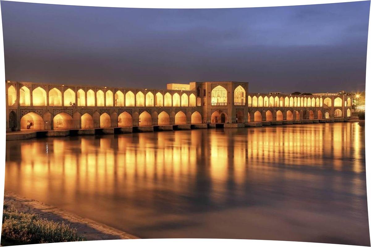
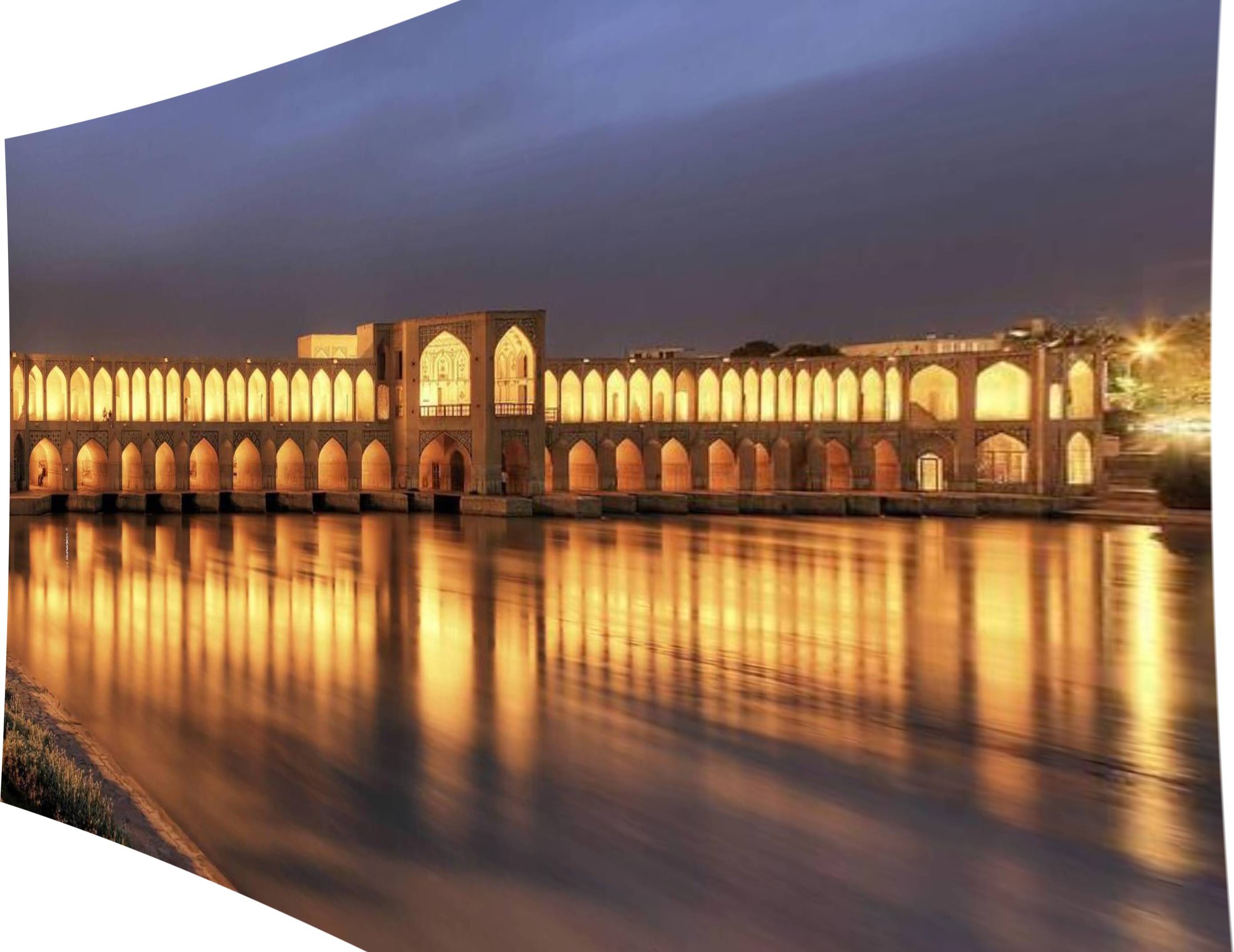
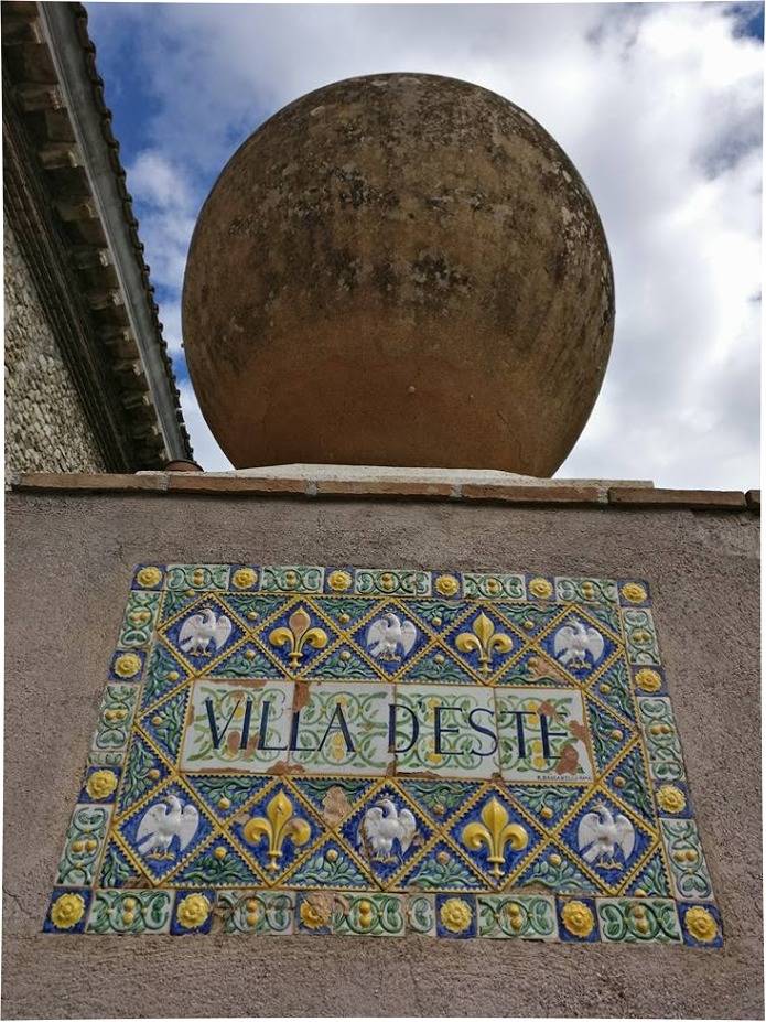
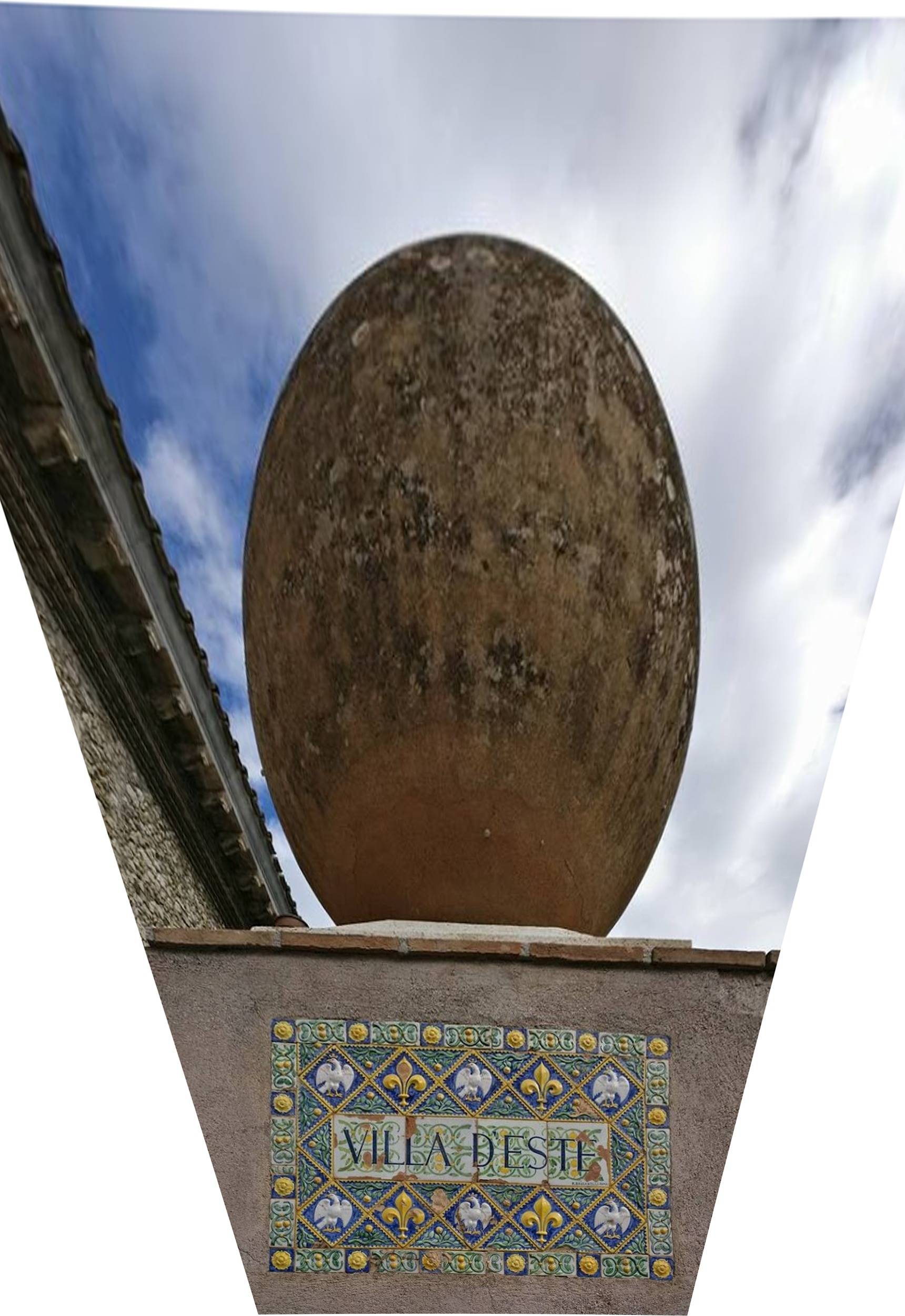
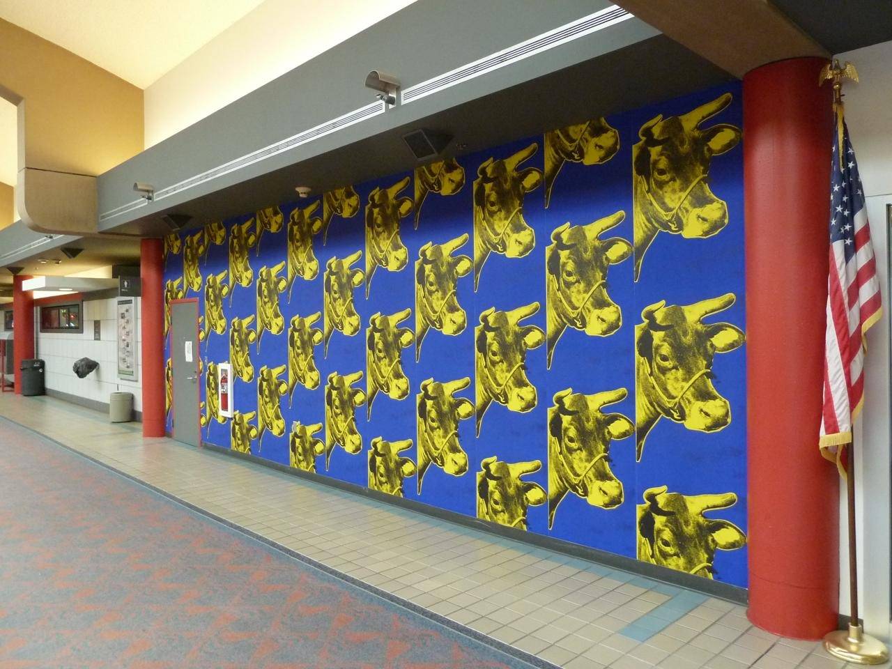
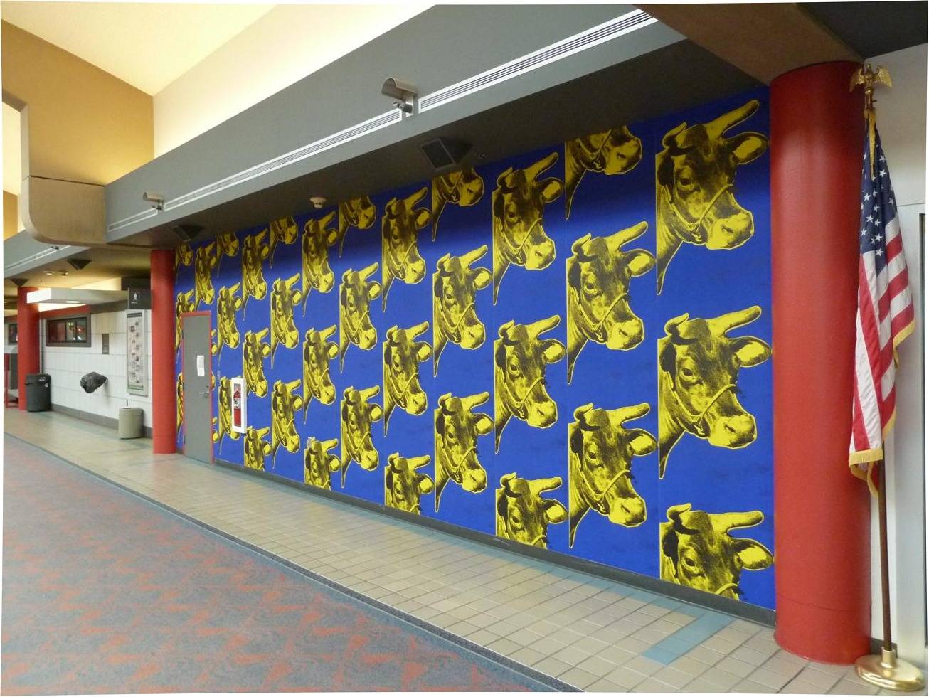
The extended real-data experiments in the following pages include (i) images with lesser radial distortion from consumer cameras and mobile phones; the images also demonstrate the proposed method’s effectiveness on diverse scene content, (ii) images for very wide field-of-view lenses (8mm and 12mm), (iii) and an additional local-optimization experiment similar to the one in Fig. 6 on a GoPro Hero 4 image taken with its medium field-of-view setting, which further demonstrates the need for a minimal solver that jointly estimates lens distortion with affine-rectification to achieve an accurate undistortions and rectifications.

Figure C.1: Narrow field-of-view and diverse scene-content experiments for $\mathtt{H}2.5\mathbf{l}\mathbf{u}\lambda$+LO. The proposed method works well if the input image has little or no radial lens distortion. This imagery is typical of consumer cameras and mobile phone cameras. The images are diverse and contain unconventional scene content. Input images are on the top row; undistorted images are on the middles row, and the rectified images are on the bottom row.

Original image

$\mathtt{H}2\mathbf{l}\mathbf{u}$+LO; $20.3\%$ inliers

$\mathtt{H}2.5\mathbf{l}\mathbf{u}\lambda$+LO; $31.2\%$ inliers

$\mathtt{H}3.5\mathbf{l}\mathbf{u}\mathbf{v}\lambda$+LO; $30.7\%$ inliers

Figure C.2: GoPro Hero 4 at the medium setting for different solvers. Results from lo-ransac (see Sec. 4) for $\mathtt{H}2\mathbf{l}\mathbf{u}$, which omits distortion, and the proposed solvers $\mathtt{H}2.5\mathbf{l}\mathbf{u}\lambda$ and $\mathtt{H}3.5\mathbf{l}\mathbf{u}\mathbf{v}\lambda$. The top row has rectifications after local optimization (LO); The bottom row has undistortions estimated from the best minimal sample. lo-ransac fails from the poor initializations by $\mathtt{H}2\mathbf{l}\mathbf{u}$ (column 2). The proposed solvers in columns 3 and 4 give a correct rectification. The bottom left has a chessboard undistorted using the division parameter estimated from the building facade by $\mathtt{H}2.5\mathbf{l}\mathbf{u}\lambda$+LO.

Figure C.3: Very wide-angle images undistorted and rectified with $\mathtt{H}2.5\mathbf{l}\mathbf{u}\lambda$+LO. The left column is an image from an 8mm lens, and the right column is from a 12mm lens. The top row contains the input images; the middle row contains the undistorted images, and the bottom row contains the rectified images. The division model [7] used for radial lens distortion has only 1 parameter, which may impose limits for modeling extreme lens distortion.

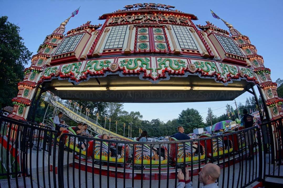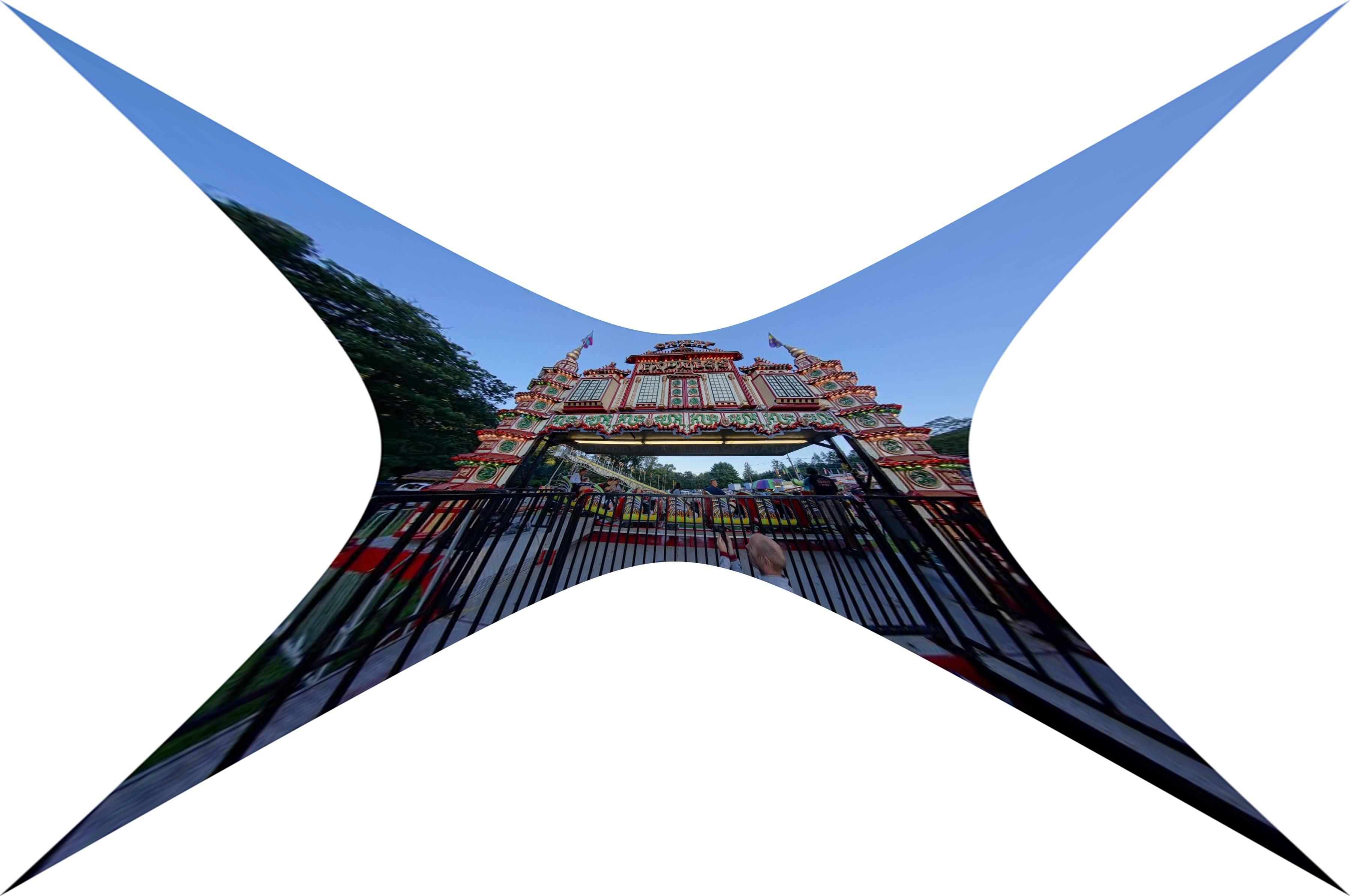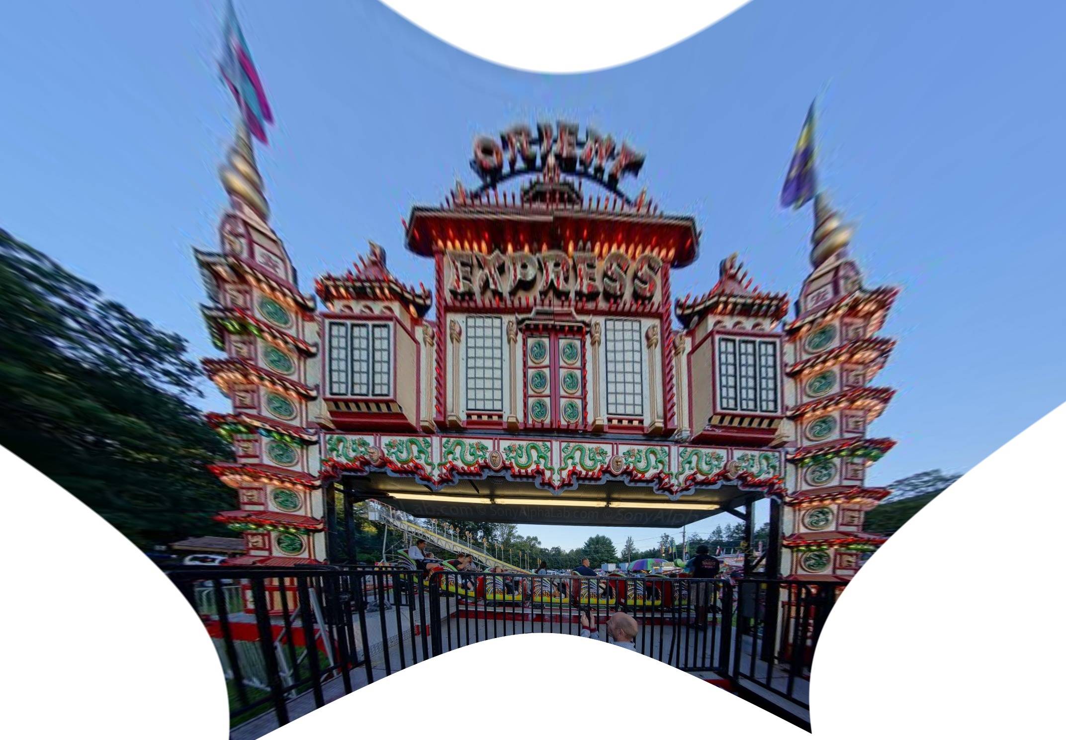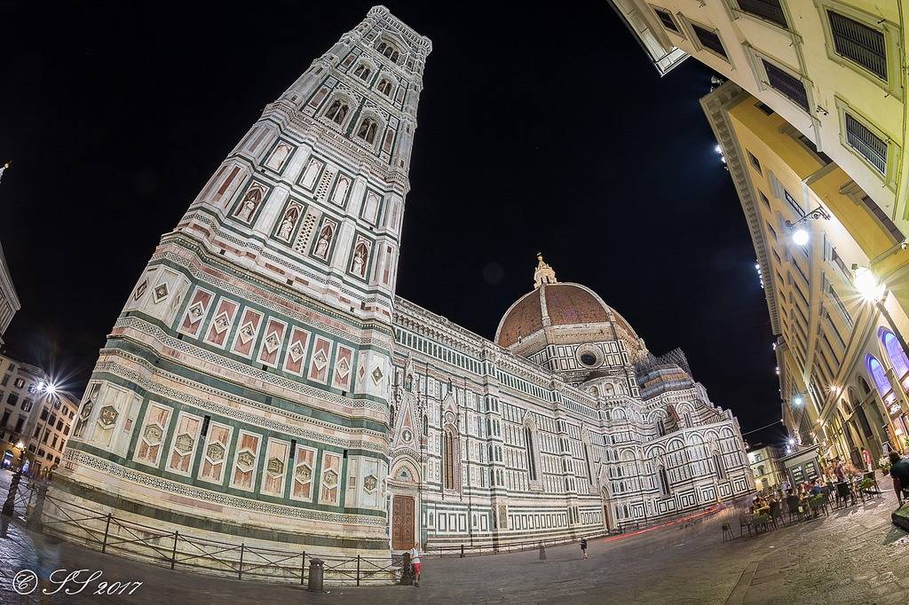Affine-covariant feature detections

Inlying affine-covariant features

Undistorted

Undistorted and rectified

Figure C.4: Problem difficulty and method robustness The input to the method is ungrouped affine-covriant features (top left). Common problems include missed detections of repeated texture, duplicate detections, and detections due to compression artifacts, all of which are visible in this example. The inliers with respect to the total number of detected features can be a very small proportion (top right). Still the method can estimate accurate undistortion (bottom left) and affine rectification (bottom right) even from a very sparse sampling of the inlying affine-covariant features on the scene plane (top right).

References

- [1] D. Aiger, D. Cohen-Or, and N. Mitra. Repetition maximization based texture rectification. Computer Graphics Forum, 31(2):439–448, 2012.
- [2] M. Antunes, J. P. Barreto, D. Aouada, and B. Ottersten. Unsupervised vanishing point detection and camera calibration from a single manhattan image with radial distortion. In CVPR, July 2017.
- [3] R. Arandjelović and A. Zisserman. Three things everyone should know to improve object retrieval. In CVPR, 2012.
- [4] O. Chum and J. Matas. Planar affine rectification from change of scale. In ACCV, 2010.
- [5] O. Chum, J. Matas, and v. Obdržálek. Enhancing RANSAC by generalized model optimization. In ACCV, 2004.
- [6] D. Cox, J. Little, and O. D. Using algebraic geometry. Springer, 2004.
- [7] A. W. Fitzgibbon. Simultaneous linear estimation of multiple view geometry and lens distortion. In CVPR, 2001.
- [8] D. R. Grayson and M. E. Stillman. Macaulay 2, a software system for research in algebraic geometry, 2002.
- [9] R. I. Hartley and A. W. Zisserman. Multiple View Geometry in Computer Vision. Cambridge University Press, ISBN: 0521540518, second edition, 2004.
- [10] Z. Kukelova, M. Bujnak, and T. Pajdla. Automatic generator of minimal problem solvers. In ECCV, 2008.
- [11] Z. Kukelova, J. Heller, B. M., and T. Pajdla. Radial distortion homography. In CVPR, 2015.
- [12] V. Larsson, K. Åström, and M. Oskarsson. Efficient solvers for minimal problems by syzygy-based reduction. In CVPR, 2017.
- [13] V. Larsson, K. Åström, and M. Oskarsson. Polynomial solvers for saturated ideals. In ICCV, 2017.
- [14] D. Lowe. Distinctive image features from scale-invariant keypoints. IJCV, 60(2):91–110, 2004.
- [15] M. Lukáč, D. Sýkora, K. Sunkavalli, E. Shechtman, O. Jamriška, N. Carr, and T. Pajdla. Nautilus: Recovering regional symmetry transformations for image editing. ACM Trans. Graph., 36(4):108:1–108:11, July 2017.
- [16] J. Matas, O. Chum, M. Urban, and T. Pajdla. Robust wide baseline stereo from maximally stable extremal regions. In BMVC, 2002.
- [17] K. Mikolajczyk and C. Schmid. A performance evaluation of local descriptors. PAMI, 2004.
- [18] K. Mikolajczyk and C. Schmid. Scale and affine invariant interest point detectors. volume 60, 2004.
- [19] D. Mishkin, F. Radenovic, and J. Matas. Learning discriminative affine regions via discriminability. CoRR, abs/1711.06704, 2017.
- [20] Š. Obdržálek and J. Matas. Object recognition using local affine frames on distinguished regions. In BMVC, 2002.
- [21] J. Pritts, O. Chum, and J. Matas. Detection, rectification and segmentation of coplanar repeated patterns. In 2014 IEEE Conference on Computer Vision and Pattern Recognition, 2014.
- [22] J. Pritts, D. Rozumnyi, M. P. Kumar, and O. Chum. Coplanar repeats by energy minimization. In BMVC, 2016.
- [23] F. Schaffalitzky and A. Zisserman. Geometric grouping of repeated elements within images. In BMVC, 1998.
- [24] A. Vedaldi and B. Fulkerson. VLFeat: An open and portable library of computer vision algorithms. http://www.vlfeat.org/, 2008.
- [25] H. Wildenauer and B. Micusík. Closed form solution for radial distortion estimation from a single vanishing point. In BMVC, 2013.
- [26] C. Wu, J. M. Frahm, and M. Pollefeys. Repetition-based dense single-view reconstruction. In CVPR, 2011.
- [27] Z. Zhang, A. Ganesh, X. Liang, and Y. Ma. TILT: transform invariant low-rank textures. IJCV, 99(1):1–24, 2012.