A recurrent neural network for classification of unevenly sampled variable stars

Abstract

Astronomical surveys of celestial sources produce streams of noisy time series measuring flux versus time (“light curves”). Unlike in many other physical domains, however, large (and source-specific) temporal gaps in data arise naturally due to intranight cadence choices as well as diurnal and seasonal constraints [1, 2, 3, 4, 5]. With nightly observations of millions of variable stars and transients from upcoming surveys [4, 6], efficient and accurate discovery and classification techniques on noisy, irregularly sampled data must be employed with minimal human-in-the-loop involvement. Machine learning for inference tasks on such data traditionally requires the laborious hand-coding of domain-specific numerical summaries of raw data (“features”) [7]. Here we present a novel unsupervised autoencoding recurrent neural network [8] (RNN) that makes explicit use of sampling times and known heteroskedastic noise properties. When trained on optical variable star catalogs, this network produces supervised classification models that rival other best-in-class approaches. We find that autoencoded features learned on one time-domain survey perform nearly as well when applied to another survey. These networks can continue to learn from new unlabeled observations and may be used in other unsupervised tasks such as forecasting and anomaly detection.

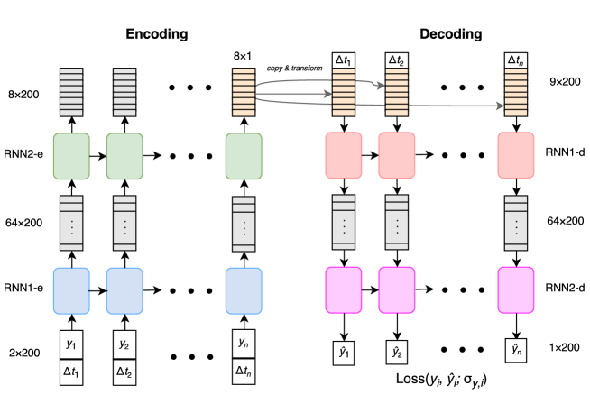
The RNN feature extraction architecture proposed (Fig. 1) consists of two components: an encoder, which takes a time series as input and produces a fixed-length feature vector as output, and a decoder, which translates the feature vector representation back into an output time series. The principal advantages of our architecture over a standard RNN autoencoder [8] are the eative handling of the sampling times and the explicit use of measurement uncertainty in the loss function.

Specifically, the autoencoder network is trained with times and measurements as inputs and those same measurement values as outputs. The mean squared reconstruction error of the output sequence is minimized, using backpropagation and gradient descent. In the case where individual measurement errors are available, the reconstruction error at each time step can be weighted (in analogy with standard weighted least squares regression) to reduce the penalty for reconstruction errors when the measurement error is large (see Methods).

The feature vector is then taken to be the last element of the output sequence of the last encoder layer, so its dimension is equal to the number of hidden units in that layer. The fixed-length embedding vector produced by the encoder contains sufficient information to approximately reconstruct the input signal, so it may be thought of as a low-dimensional feature representation of the input data. Although we focus here on an autoencoder model for feature extraction, the decoder portion of the network can also be trained directly to solve classification or regression problems, as described in detail in the Supplementary Information (SI).

To investigate the utility of the automatically extracted features, we train an autoencoder model to reconstruct a set of (unlabeled) light curves and then use the resulting features to train a classifier to predict the variable star class. Here we use the 50,124 light curves from the All Sky Automated Survey (ASAS) Catalog of Variable stars [2]. The autoencoder is trained using the full set of both labeled and unlabeled light curves, and the resulting features are then used to build a model to solve the supervised classification task. We compare the resulting classifier to a model which uses expert-chosen features and demonstrate that the autoencoding features perform at least as well, and in some cases better, than the hand-selected features.

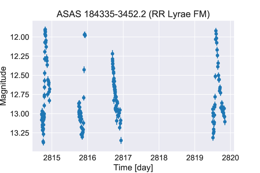
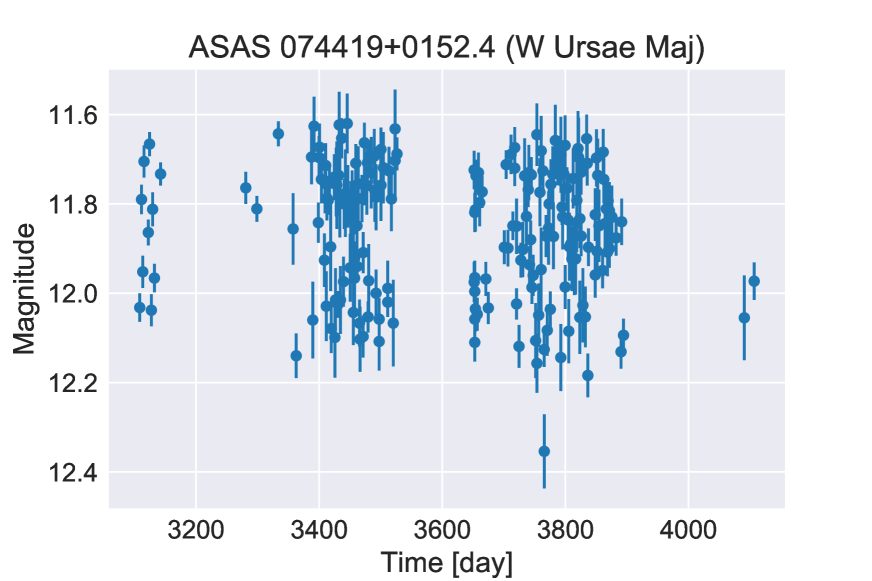
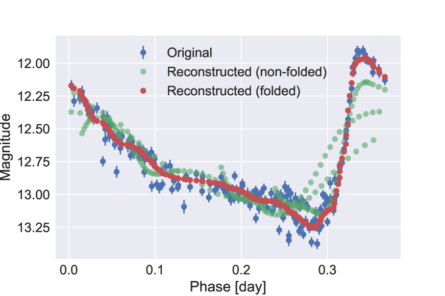
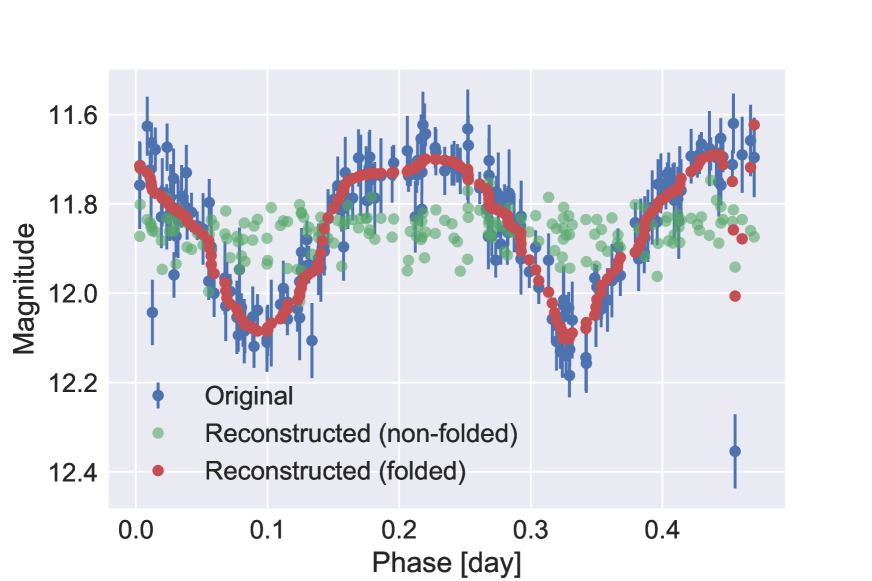
Figure 2 depicts some examples of reconstructed light curves for an embedding of length 64 (the other parameters of the autoencoder are described in Methods); the examples are chosen to represent the 25th and 75th percentile of reconstruction error in order to show the range of different qualities of reconstruction. The model is able to effectively represent light curves which exhibit relatively smooth behavior, even in the presence of large gaps between samples; however, curves that vary more rapidly (i.e., those with small periods) are less likely to be reconstructed accurately. As such we also trained an autoencoder model on the period-folded values (replacing time with phase) using the measured periods [9]. Figure 2 shows that the resulting reconstructions are improved, especially in the case of the low-period signal. The effect of period on the accuracy of autoencoder reconstructions is explored further using simulated data (see SI). In what follows, we use autoencoders trained on period-folded light curve data.

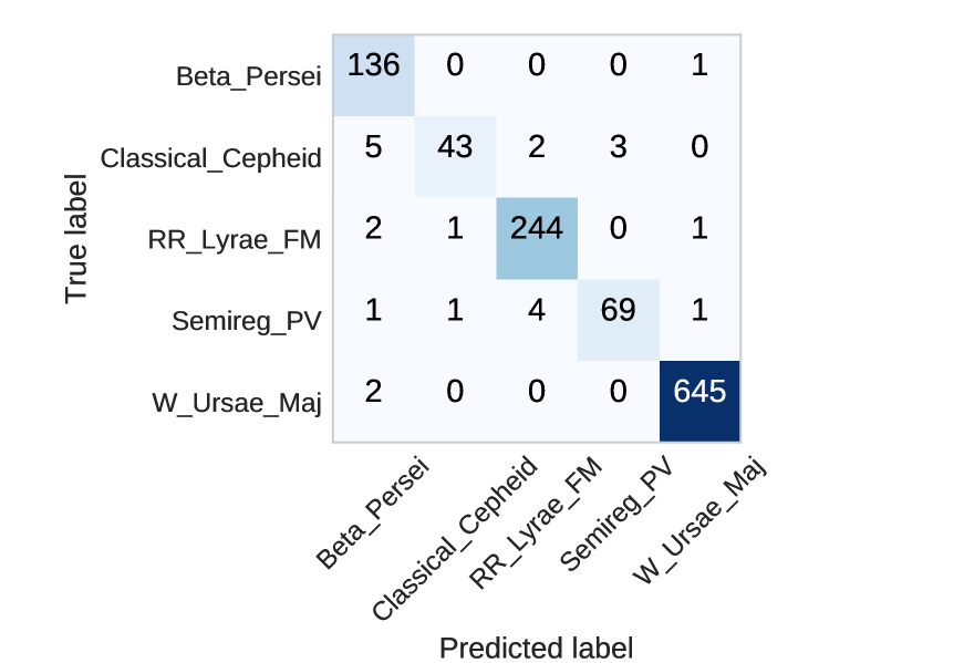
To evaluate the usefulness of our features for classification, we identify a subset of ASAS light curves from five classes of variable stars (see Methods for details). We then train a random forest classifier [17] using the autoencoder-generated features for 80% of the samples from each class, along with the means and standard deviations of each light curve which are removed in preprocessing (see Methods). The resulting estimator achieves 98.8% average accuracy on the validation sets across five 80/20 train/validation splits.

As a baseline, we also constructed random forest classifiers using two sets of standard features for variable star classification. The first are the features used in Richards et al. [11] (henceforth abbreviated “Richards et al. features”); the features are implemented in the Cesium ML project [12] and also as part of the FATS package [13]. These features have been used by numerous studies (e.g., refs [14, 15, 16]) including state-of-the-art classification performance on the ASAS survey and remain competitive against other classification methods [17]. The second set of features consists of those used by Kim & Bailer-Jones [18] (henceforth referred to “Kim/Bailer-Jones features”) and implemented in the Upsilon package. Some features are shared between the two, and each set of features is an aggregation of features from many different works. In both cases we use the same hyperparameter selection technique described in Figure 3.

The Richards et al. features achieve the best average validation accuracy at 99.4% across the same five splits, as shown in Table 1. However, it is worth noting that the same features were also used in the labeling of the training set [9], so it is not surprising that they achieve almost perfect classification accuracy for this problem. The Kim/Bailer-Jones features, which may provide a more natural baseline, achieve 98.8% validation accuracy, comparable to that of the autoencoder model.

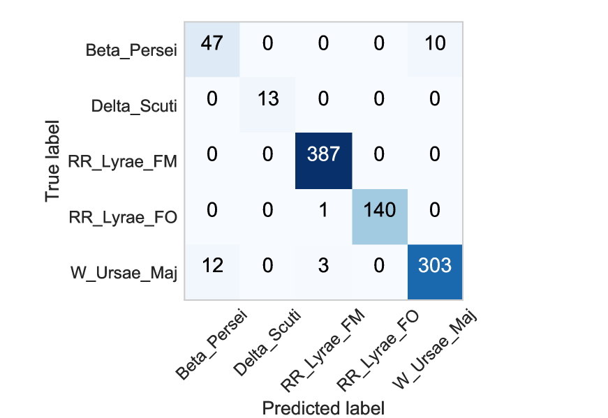
Our second example applies the same feature extraction methodology to variable star light curves from the Lincoln Near-Earth Asteroid Research (LINEAR) survey [19, 20]. The LINEAR dataset consists of 5,204 labeled light curves from five classes of variable star (see Methods for details). Unlike in the ASAS example above, here all the available light curves are labeled, so there is no additional unlabeled data to leverage in order to improve the quality of the extracted features. We find that the autoencoder features outperform the Richards et al. features by 0.38% and the Kim/Bailer-Jones features by 1.61% (see Table 1). In particular, the autoencoder-based model correctly classifies all but 1 RR Lyrae, suggesting that perhaps some autoencoder features could help improve the performance of the Richards et al. or Kim/Bailer-Jones features for that specific discrimination task.

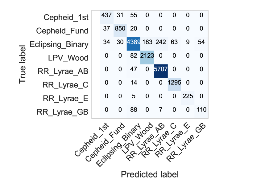
Finally, we followed the same procedure to train an autoencoder and subsequently a random forest classifier to predict the classes of 21,474 variable stars from the MACHO catalog [21]. Once again, our autoencoder approach achieves the best validation accuracy of the three methods considered, averaging 93.6% compared to 90.5% and 89.0% for the Richards et al. and Kim/Bailer-Jones feature sets, respectively.

As shown, training a autoencoder RNN to represent time series sequences can produce informative high-level feature representations in an unsupervised setting. Rather than require fixed-length time series, our approach naturally accommodates variable length inputs. Other unsupervised techniques for feature extraction on irregular time-series data have also been developed (e.g., clustering methods [22]), but those scale quadradically in the number of training examples, whereas our approach scales linearly. Moreover, our approach explicitly accounts for measurement noise. The resulting features are shown to be comparable or better for supervised classification tasks than traditional hand-coded features. As new sources accumulate without known labels, the unsupervised and on-line nature of such networks should ensure continued model improvements in a way not possible with a fixed number of features. When metadata is also available (e.g., color and sky position for astronomical variables), features derived from such non-temporal data can be easily used in conjunction with the auto-encoded features of the time series.

While the autoencoder approach we have described is well-suited to tasks involving a relatively large amount of (labeled or unlabeled) data, future research should study the efficacy of cross-domain transfer learning, where feature representations learned from a very large dataset are applied to another problem where fewer examples are available. Another promising application is unsupervised data exploration, such as clustering; autoencoding features could be used as a generic lower-dimensional representation like t-SNE [23] to identify outliers/anomalies in new data. Autoencoders could also act as non-parametric interpolators tuned to the domain on which the models are trained. Finally, while we have focused on single-channel time series, the proposed network is easily extensible to multi-channel time series data as well as multi-dimensional time series, such as unevenly sampled sequential imaging.

Author information

Contributions

B.N. implemented and trained the networks, assembled the machine learning results, and generated the first drafts of the paper and figures. J.S.B. conceived of the project, assembled the astronomical light curves, and oversaw the supervised training portions. F.P. provided theoretical input. S.vdW. discussed the results and commented on the manuscript.

Affiliations

Department of Astronomy, University of California, Berkeley, CA 94720, USA.
B. Naul, J. S. Bloom

Department of Statistics, Berkeley, CA 94720, USA.
F. Pérez

Berkeley Institute for Data Science, University of California, Berkeley, CA 94720, USA.
S. van der Walt

Corresponding author

Correspondence to B. Naul.

Figure 1: Diagram of an RNN encoder/decoder architecture for irregularly sampled time series data. This network uses two RNN layers (specifically, bidirectional gated recurrent units (GRU) [6, 25]) of size 64 for encoding and two for decoding, with a feature embedding size of 8. The encoder takes as inputs the measurement values as well the sampling times (more specifically, the differences between sampling times); the sequence is processed by a hidden recurrent layer to produce a new sequence, which can then be used as the input to another hidden recurrent layer, etc. The fixed-length embedding is constructed by passing the output of the last recurrent layer into a single fully-connected layer with linear activation function and the desired output size. The decoder first repeats the fixed-length embedding $n_{T}$ times, where $n_{T}$ is the length of the desired output sequence, and then appends the sampling time differences to the corresponding elements of the resulting vector sequence. The sampling times are passed to both the encoder and decoder; the feature vector characterizes the functional form of the signal, but the sampling times are needed to determine the points at which that function should be evaluated. The remainder of the decoder network is another series of recurrent layers, with a final linear layer to generate the output sequence. We also apply 25% dropout [14] between recurrent layers, which we omit from the figure for simplicity. In our model we take the number and size of recurrent layers in the encoder and decoder modules to be equal, but in general the two components are entirely distinct and need not share any architectural similarities.

(a) 25th percentile

(b) 75th percentile

(c) 25th percentile (folded)

(d) 75th percentile (folded)

Figure 2: Example autoencoder reconstructions of ASAS light curves from 64-dimensional feature representation. Twenty-fifth and seventy-fifth percentile error reconstructions are shown for raw, unfolded light curves in a) and b), and for period-folded light curves in c) and d). The $\sim$V-band magnitudes are in the Vega system.

(a) ASAS

(b) LINEAR

(c) MACHO

Figure 3: Confusion matrices for autoencoder-feature random forest classifiers for labeled variable star light curves from a) ASAS, b) LINEAR, and c) MACHO surveys. Values along the diagonals are counts of correctly-classified light curves, and off-diagonal values correspond to incorrect classifications (darker squares correspond to higher counts).

	ASAS	LINEAR	MACHO
Autoencoder	$98.77\%\pm 0.39\%$	$97.10\%\pm 0.60\%$	$93.59\%\pm 0.15\%$
Richards et al.	$99.42\%\pm 0.27\%$	$96.72\%\pm 0.67\%$	$90.50\%\pm 0.22\%$
	($+0.66\pm 0.49$)%	($-0.37\pm 0.45$)%	($-2.74\pm 0.16$)%
Kim/Bailer-Jones	$98.83\%\pm 0.33\%$	$95.49\%\pm 0.83\%$	$88.98\%\pm 0.19\%$
	($+0.06\pm 0.32$)%	($-1.60\pm 0.59$)%	($-4.60\pm 0.16$)%

Table 1: Validation accuracies (mean $\pm$ standard deviation across five stratified cross-validation splits) for the autoencoder, Richards et al., and Kim/Bailer-Jones feature random forests. Note that the training labels for the ASAS data were identified in part using the Richards et al. features. In parentheses are the mean and standard deviation of the differences in accuracy (Other Method - Autoencoder; a negative value means the autoencoder performed better) over the cross-validation folds.

Methods

We describe here the implementation specifics of the proposed neural network classifier, and the detailed properties of the datasets which were used in the above experiments.

Comparison with other neural network approaches

Many of the most commonly used approaches for time series analysis, including standard recurrent neural networks, rely on an implicit assumption that the data is uniformly sampled in time. This assumption is not unique to neural network approaches: the Fast Fourier Transform (FFT), commonly used in featurization, is only well-defined for the evenly sampled, homoskedastic case. Existing neural networks that do allow for uneven sampling operate on interpolations of the data (see, e.g., [2, 3, 4]), thereby replacing the problem with one that can be solved by standard approaches. Any form of interpolation makes implicit assumptions about the spectral structure of the data, which may be unjustified and can end up introducing biases and artifacts. These artifacts increase with sampling unevenness and are ultimately properties of the algorithm, not the data.

Loss function for known measurement errors

Typically an autoencoder is trained to minimize the difference between the input and the reconstructed values, usually in terms of mean squared error. In the case of astronomical surveys, individual measurement errors are generally available for each time step. We therefore constructed a new loss function which weighs the reconstruction error at each time step more or less heavily when the measurement errors are small or large, respectively (in analogy with standard weighted least squares regression). In particular, our models are trained to minimize the weighted mean squared error

$$\textrm{WMSE}=\frac{1}{n_{T}}\sum_{i=1}^{N}\sum_{j=1}^{n_{T}}\left(y_{i}^{(j)}-\hat{y}_{i}^{(j)}\right)^{2}/\left(\sigma_{i}^{(j)}\right)^{2},$$ (1)

where $n_{T}$ is the length of the sequences, $N$ the number of light curves, and $y_{i}^{(j)},$ $\hat{y}_{i}^{(j)},$ and $\sigma_{i}^{j}$ are (respectively) the $j$th measurement, reconstruction value, and measurement error of the $i$th light curve.

Neural network parameters

The autoencoders used for the ASAS and LINEAR survey classification tasks were constructed using a network architecture like that of Fig. 1, consisting of two encoding and two decoding GRU layers of size 96, and an embedding size of 64. The network is trained using the Adam optimizer with learning rate $\lambda=5\times 10^{-4}$ to minimize the weighted mean squared reconstruction error defined in Eq. (1).

Random forest classifier parameters

In the classification experiments, a random forest classifier is trained to predict the class of each labeled light curve from either the unsupervised autoencoder features from our method, or the baseline features from [11]. The hyperparameters of the random forest were chosen by performing a five-fold cross validation grid search over the following grid: $n_{\textrm{trees}}\in\{50,100,250\},\textrm{criterion}\in\{\textrm{gini,entropy}\},\textrm{max features}\in\{3,6,12,18\},\textrm{min leaf samples}\in\{1,2,3\}$. In each case, 80% of the available samples are used as training data, and 20% are withheld as test data (the hyperparameter selection is performed only using the training data); the same splits are used for the autoencoder and Richards et al. features, and in each case we present the results across five different choices of train/test splits.

All Sky Automated Survey (ASAS) data

The ASAS Catalog of Variable stars [2] consists of 50,124 (mostly unlabeled) variable star light curves. For the ASAS dataset, we select 349 Beta Persei, 130 Classical Cepheids, 798 RR Lyrae (FM), 184 Semiregular PV, and 181 W Ursae Major class stars. The class label of each star is either either manually identified or predicted with high probability ($>$99%) by the Machine-learned ASAS Classification Catalog, and periods used in period-folding were identified programmatically as described in [9].

Lincoln Near-Earth Asteroid Research (LINEAR) data

The LINEAR dataset consists of 5,204 light curves from five classes of star: 2,234 RR Lyrae FM, 1,860 W Ursae Major, 749 RR Lyrae FO, 291 Beta Persei, and 70 Delta Scuti. All of the light curves in the LINEAR dataset were manually classified, and periods used for period-folding were validated manually as described in [20].

Massive Compact Halo Object (MACHO) Project data

The MACHO dataset consists of 21,474 light curves from eight classes of star: 7,405 RR Lyrae AB, 6,835 Eclipsing Binary, 3,049 Long-Period Variable Wood (subclasses A-D were combined into a single superclass), 1,765 RR Lyrae C, 1,185 Cepheid Fundemantal, 683 Cepheid First Overtone, 315 RR Lyrae E, and 237 RR Lyrae/GB Blend. All models were trained on brightness and error values from the red band, though the same approaches could be used on the blue band or both bands simultaneously. Periods and labels were determined using a semi-automated procedure as described in [21]. The full MACHO dataset also contains light curves from many more non-variable sources, which were not used in training either the autoencoder or the random forests in our experiments.

Data preprocessing

We first processed the raw data from each survey as described in [9], removing low-quality measurements (those with grade C or below), so that each source consists of a series of observations of time, brightness (V-band magnitude), and measurement error values, denoted $(\bm{t}_{i},\bm{y}_{i},\bm{\sigma}_{i})$. Before training, we further preprocessed the data by centering and scaling each light curve to have mean zero and standard deviation one. We also manually removed light curves from our autoencoder training set which did not exhibit any notable periodic behavior by computing a “super smoother” [5] fit for each light curve with period equal to the estimated period from [9] and omitting light curves with residual greater than 0.7 (we observed that including aperiodic sources tended to degrade the quality of the reconstructions). Finally, we partitioned the light curves into subsequences of length 200; this is not strictly necessary since our recurrent architecture allows for input and output sequences of arbitrary length, but the use of sequences of equal length is computationally advantageous and reduces training time (see SI for details). The resulting dataset consists of 33,103 total sequences of length $n_{T}=200$.

Data availability statement

All data and code for reproducing the above experiments is available online at https://github.com/bnaul/IrregularTimeSeriesAutoencoderPaper, including Python code implementing the simulations, Jupyter notebooks for reproducing the figures, and trained autoencoder models and weights.

Supplementary information (SI)

1 Background on neural networks for time series data

Machine learning techniques for time series data typically map each sequence to a set of scalar-valued features that attempt to capture various distinguishing properties; these may range from simple summary statistics like median or maximum to parameters of complicated model fits. Features are then used as inputs to train models which map fixed-length feature vectors to the relevant labels. The process of building and selecting features can be difficult, requiring extensive expert knowledge and iterative fine-tuning, and feature generation itself may be computationally expensive. One distinct advantage of neural networks is the elimination of the need to manually create, compute, and select effective features [lecun2015deep]. Nearly all applications of neural networks to time series data rely on the assumption that samples are evenly spaced in time.

Artificial neural networks have previously been applied to many time series tasks, including classification and forecasting. The simplest approaches make use of fully connected networks (see, e.g., [1]), which treats each sequence as consisting of independent observations and thereby ignores the local temporal structure. Convolutional neural networks have also been applied to time series data with considerable success [2], in particular for the problem of speech recognition [3]. The enormous popularity of convolutional networks for image analysis has led to efficient optimization techniques and highly optimized software implementations, so convolutional networks tend to be faster and easier to train than other approaches, including recurrent networks (which our technique employs). As opposed to fully connected networks which ignore the local structure of sequences, convolutional networks are well-suited for recognizing local, short-term patterns in time series data. However, convolutional networks are less ideally suited for handling irregular sequences of unequal length. For this reason we focus on recurrent networks, which are designed to handle sequences of arbitrary length.

Recurrent networks have been found to be more difficult to train than convolutional networks due to their repeating structure, which makes them more susceptible to problems of exploding or vanishing gradients during training [4]. Another drawback of the recursive structure of recurrent networks is that recomputing the internal state for each input can lead to rapid loss of information over time and difficulty in tracking long-term dependencies; these difficulties led to the development of the popular long short-term memory (LSTM) [5] and gated recurrent unit (GRU) [6] architectures, which help information be retained over longer periods of time. Some sequence processing tasks for which recurrent neural networks have been successfully applied include recognition [7], machine translation [8], and natural language processing [9].

2 Frequency-domain characteristics of unevenly sampled time series

One important class of features that is often used in time series inference problems is frequency-domain properties, including estimates of period(s) or power spectra over some range of frequencies. By far the most common approach for transforming time series data between the time and frequency domains is the (discrete) Fourier transform (DFT). The default formulation of the DFT assumes that the data are uniformly sampled. If this assumption isn’t met, more complex approaches are required that interpolate the data onto a uniform grid [10] or project it onto spaces with fixed, predefined bandwidth. A frequently used version of the latter approach is the Lomb-Scargle periodogram [11, 12], which estimates the frequency properties of a signal using a least squares fit of sinusoids. Once the power spectrum of a signal has been estimated using one of the above methods, features such as the dominant frequencies/periods can be extracted and used in machine learning tasks such as classification.

In the next section, we demonstrate a neural network architecture which is able to infer periodic behavior directly from an irregularly sampled time series without constructing an explicit estimate of the full power spectrum.

3 Simulation study: sinusoidal data

In order to evaluate the effect of depth, hidden layer size, and other architecture choices, we first carry out a number of experiments using simulated time series data generated from a know distribution. In particular, we construct periodic functions of the form

$$f_{i}(t):=A_{i}\sin(2\pi\omega_{i}t+\phi_{i})+b_{i}$$ (2)

for randomly selected parameter values $\omega_{i}$ (frequency; we will also write $T_{i}=\omega_{i}^{-1}$ to denote period), $A_{i}$ (amplitude), $\phi_{i}$ (phase), and $b_{i}$ (offset). The parameter values are chosen as independent identically-distributed (i.i.d.) samples from the probability distributions

$$A_{i} \sim\mathcal{U}(0.5,2),$$ (3)

$$\omega_{i}^{-1}=T_{i} \sim\mathcal{U}(1,10),$$ (4)

$$\phi_{i} \sim\mathcal{U}(-\pi,\pi),$$ (5)

$$b_{i} \sim\mathcal{N}(0,1),$$ (6)

where $\mathcal{U}(a,b)$ is the uniform distribution on $[a,b]$, and $\mathcal{N}(\mu,\sigma^{2})$ is the normal distribution with mean $\mu$ and variance $\sigma^{2}$. For each periodic function, we generate a set of $n_{T}=200$ sampling times $(t_{i}^{(1)},\dots,t_{i}^{(n_{T})})$ by sampling the differences from a heavy-tailed power law distribution $t_{i}^{(j+i)}-t_{i}^{(j)}\sim\operatorname{Lomax}(0.05,2)$, where the $\operatorname{Lomax}(\lambda,\alpha)$ distribution has probability density function

$$f(x;\lambda,\alpha)=\frac{\alpha}{\lambda}\left(1+\frac{x}{\lambda}\right)^{-\left(\alpha+1\right)}.$$

The resulting distribution of times is such that the mean total time is $E[t_{n_{T}}]=10$ but the sequence $(t_{i}^{(1)},\dots,t_{i}^{(n_{T})})$ is highly unevenly sampled and may contain many large gaps between consecutive samples.

Our training dataset consists of $N_{\textrm{train}}=50,000$ periodic functions and sampling time sequences generated using the above procedures; we also add white Gaussian random noise $\bm{\epsilon}_{i}^{(j)}\sim\mathcal{N}(0,\sigma^{2})$ with $\sigma=0.5$ to each measurement, so the final input data has the form

$$\bm{t}_{i}=(t_{i}^{(1)},\dots,t_{i}^{(n_{T})}),\ \bm{y}_{i}=(f_{i}(t_{i}^{(1)})+\epsilon_{i}^{(1)},\dots,f_{i}(t_{i}^{(n_{T})})+\epsilon_{i}^{(1)}).$$ (7)

Supplementary Figure 4 shows examples of randomly generated periodic functions and randomly selected points with added noise.

(a)

(b)

(c)

Supplementary Figure 4: Examples of randomly generated periodic functions. Panels a), b) and c) each contain values of a sinusoidal function with random parameters evaluated at random times. The distributions of the parameters are given in (3)–(7).

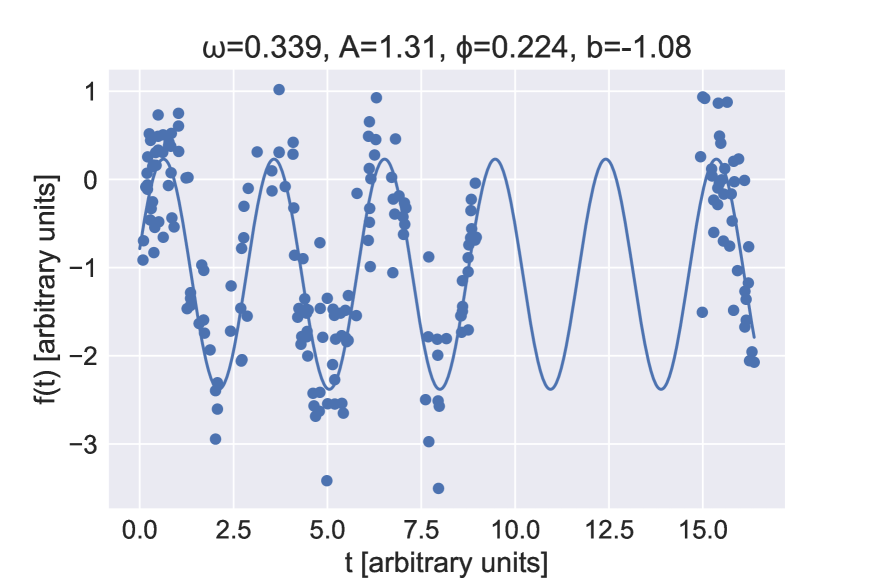
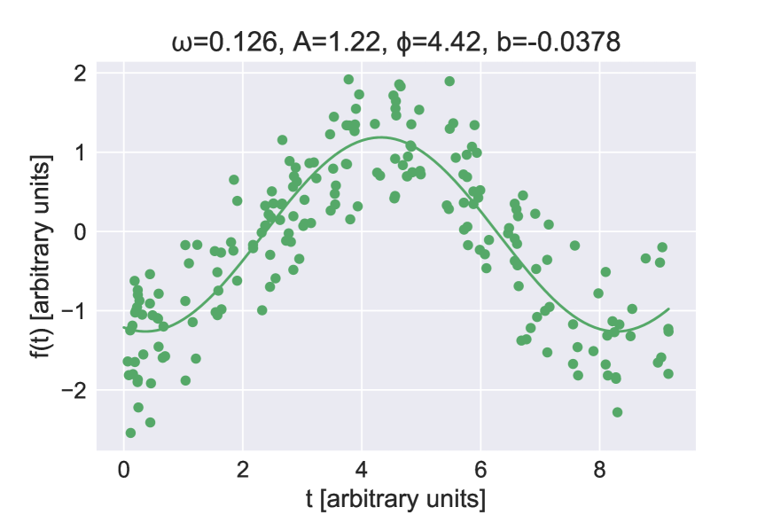
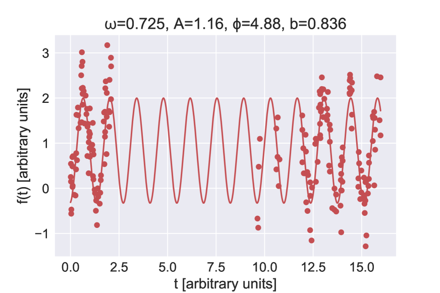
The accuracies and losses for each model are evaluated using a separate dataset of $N_{\textrm{valid}}=10,000$ sequences generated using the same methodology.

3.1 Estimating period, phase, amplitude, offset

As our initial experiment, we implement a network which solves a supervised regression problem of estimating the parameters $\bm{\theta}_{i}=(\omega_{i},A_{i},\phi_{i},b_{i})$ [as defined in (2)] from the generated times and measurement values. The corresponding network consists of the encoder portion of the network shown in Supplementary Figure 1 of the main text with an output size of four. The network is trained to minimize the mean squared error

$$\textrm{MSE}=\frac{1}{N_{\textrm{train}}}\sum_{i=1}^{N_{\textrm{train}}}\|\theta_{i}-\hat{\theta}_{i}\|_{2}^{2}$$ (8)

for the given training data; the target values are first preprocessed by re-parametrizing $\bm{\theta}_{i}$ as $(T_{i},A_{i}\cos\phi_{i},A_{i}\sin\phi_{i},b_{i})$ (which leads to faster convergence) and then centering and scaling each target variable to have mean 0 and standard deviation 1. Our network is trained via the Adam optimization method [13] with standard parameter values $\beta_{1}=0.9,\beta_{2}=0.999$ using a learning rate of $\eta=5\times 10^{-4}$ and a batch size of 500. We also impose 25% dropout [14] between recurrent layers for regularization, which does not seem to be necessary for this simple task but is beneficial for the astronomical classification tasks discussed in the main text. All models were implemented in Python using the Keras library [15] and trained using an NVIDIA Tesla K80 GPU.

(a) By epoch

(b) By time

Supplementary Figure 5: Comparison of validation losses during training for various numbers and types of layers on the periodic parameters $\bm{\theta}_{i}$. The loss plotted is the mean squared error over the validation set of the parameters being estimated as a function of a) training epoch and b) training wall time. Each colored line corresponds to a specific network architecture (layer type, layer size, and network depth) as shown in the legend: for example, “GRU(64) $\times$ 2” denotes two decoder GRU layers each composed of 64 hidden units.

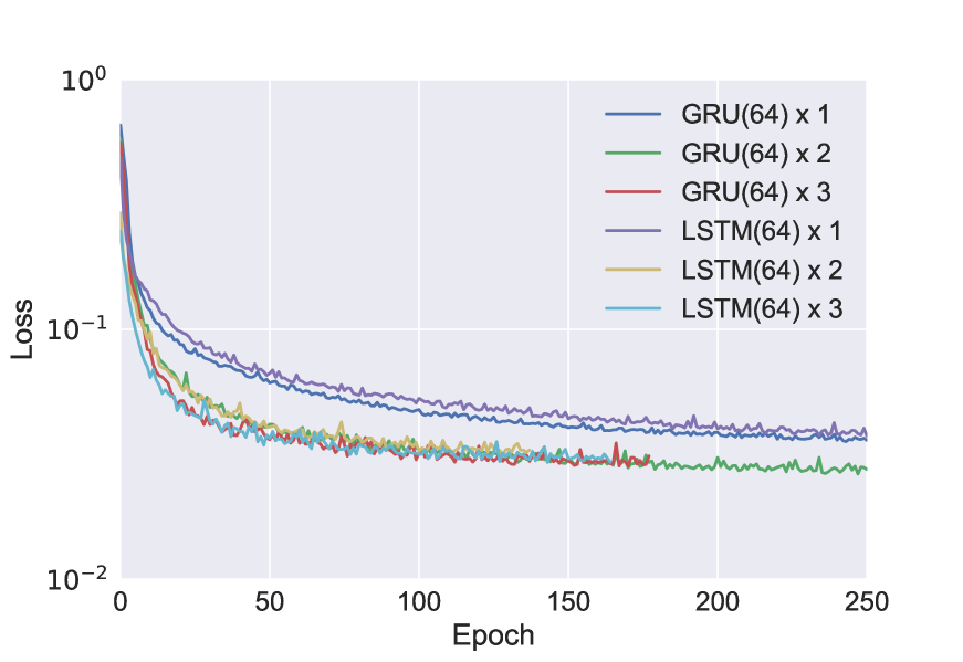
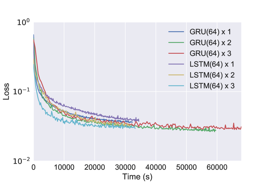
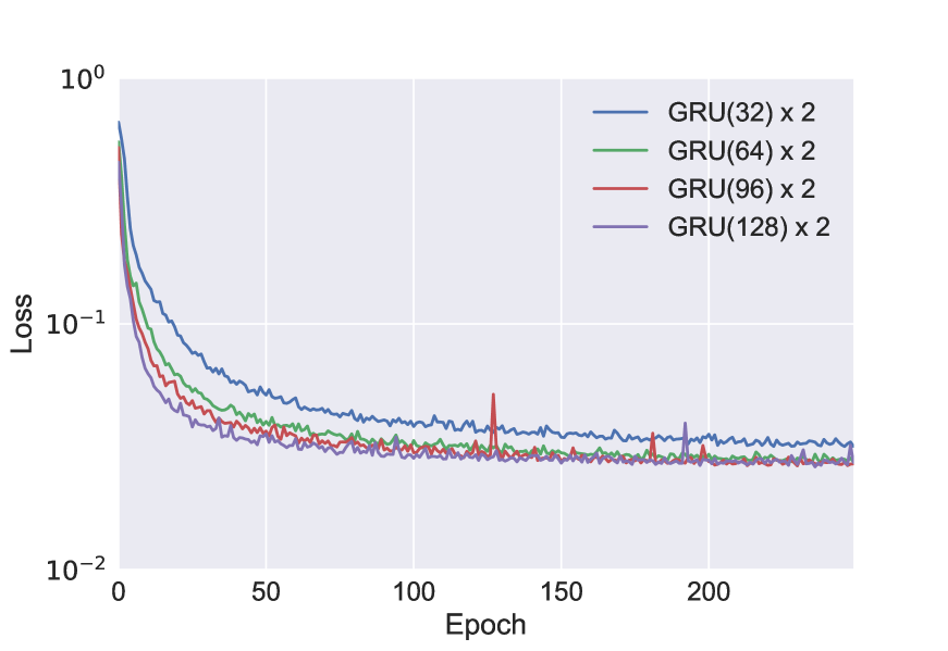
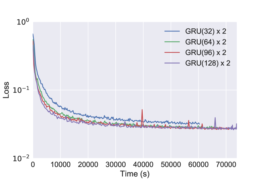
As seen in Supplementary Figures 5 and 6, the maximum accuracy achieved by the one layer networks is somewhat inferior to that of the multi-layer networks; nevertheless, it is clear that all of the architectures considered are able to accurately recover information about the periodic characteristics of the unknown functions, even in the presence of noise and sampling irregularity.

(a) By time

(b) By epoch

Supplementary Figure 6: Comparison of validation losses during training for various sizes of layers on the periodic parameters $\bm{\theta}_{i}$. The loss plotted is the mean squared error over the validation set of the parameters being estimated as a function of a) training epoch and b) training wall time. Each colored line corresponds to a specific network architecture (layer type, layer size, and network depth) as shown in the legend: for example, “GRU(64) $\times$ 2” denotes two decoder GRU layers each composed of 64 hidden units.

Supplementary Figure 14 depicts three realizations of the light curve resampling process described above.

Supplementary Figure 7: Comparison of period estimate residuals $T_{i}-\hat{T}_{i}$ for GRU and Lomb-Scargle models. Each point on the scatter plot represents the error of the predicted period from each model; the histograms on the top and right show the overall distributions of errors across all samples for the GRU and Lomb-Scargle models, respectively.

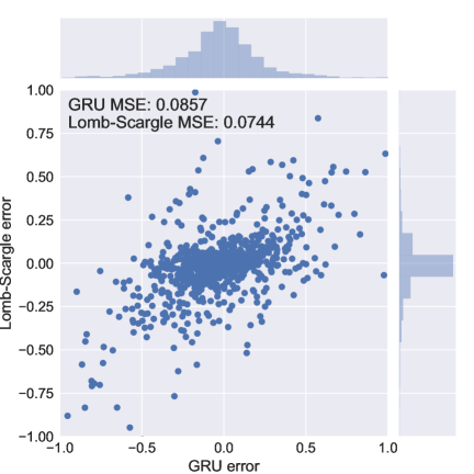
Supplementary Figure 7 compares the accuracy of an RNN estimator with two 96-unit GRU layers (ignoring the other estimated parameters besides the period) with that of a Lomb-Scargle estimate of the period, which has well-understood statistical convergence properties [16]. The accuracy of the two models is comparable, with the Lomb-Scargle estimate performing slightly better for this particular case. In the next we estimate the same periodic parameters using a semi-supervised approach based on autoencoder features.

3.2 Inferring periodic parameters from autoencoding features

For the same simulated $N_{\textrm{train}}$ periodic sequences generated above, we now train a full encoder-decoder network as depicted in Supplementary Figure 1 of the main text and attempt to recover the parameters $\omega_{i},A_{i},\phi_{i}$, and $b_{i}$ from the encoding $\bm{v}_{i}$. Instead of minimizing a loss function for the parameters themselves, we now train the network to minimize the mean squared reconstruction error

$$\textrm{MSE}=\frac{1}{N_{\textrm{train}}n_{T}}\sum_{i=1}^{N_{\textrm{train}}}\sum_{j=1}^{n_{T}}\left(f_{i}(t_{i}^{(j)})-\hat{y}_{i}^{(j)}\right)^{2}.$$ (9)

Note that reconstruction target is the original (de-noised) periodic function, not to the raw measurement values.

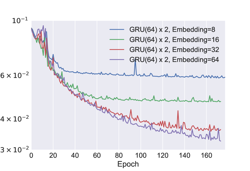
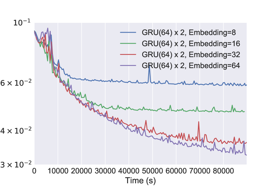
The autoencoder model has an additional hyperparameter (compared to the encoder for directly estimating the periodic parameters) of the size of embedding to use for the encoding layer. Supplementary Figure 8 shows the reconstruction accuracy for a fixed encoder and decoder architecture, with each consisting of two bidirectional GRU layers of size 64, for a range of embedding sizes.

(a) By epoch

(b) By time

Supplementary Figure 8: Comparison of GRU autoencoder validation losses during training for various embedding sizes. The loss plotted is the mean squared error over the validation set of the reconstructed sequences as a function of a) training epoch and b) training wall time. Each colored line corresponds to a different dimensionality of embedding: for example, “GRU(64) $\times$ 2, Embedding=8” denotes two encoder and two decoder GRU layers each composed of 64 hidden units, with an embedding layer of dimension 8 inbetween.

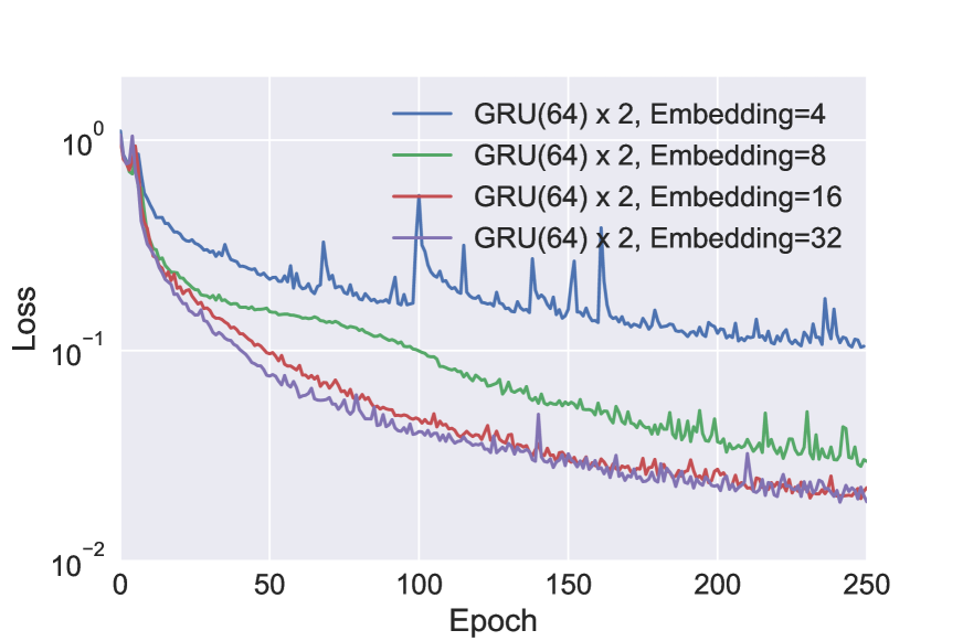
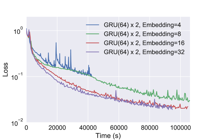
Although each target function can be fully characterized in terms of four parameters, it is clear that increasing the embedding size does improve the accuracy of the reconstruction up to a point. However, given a longer training time or different choice of learning rate, it is conceivable that a model with only four embedding values could achieve the same level of accuracy as those with higher-dimensional representations.

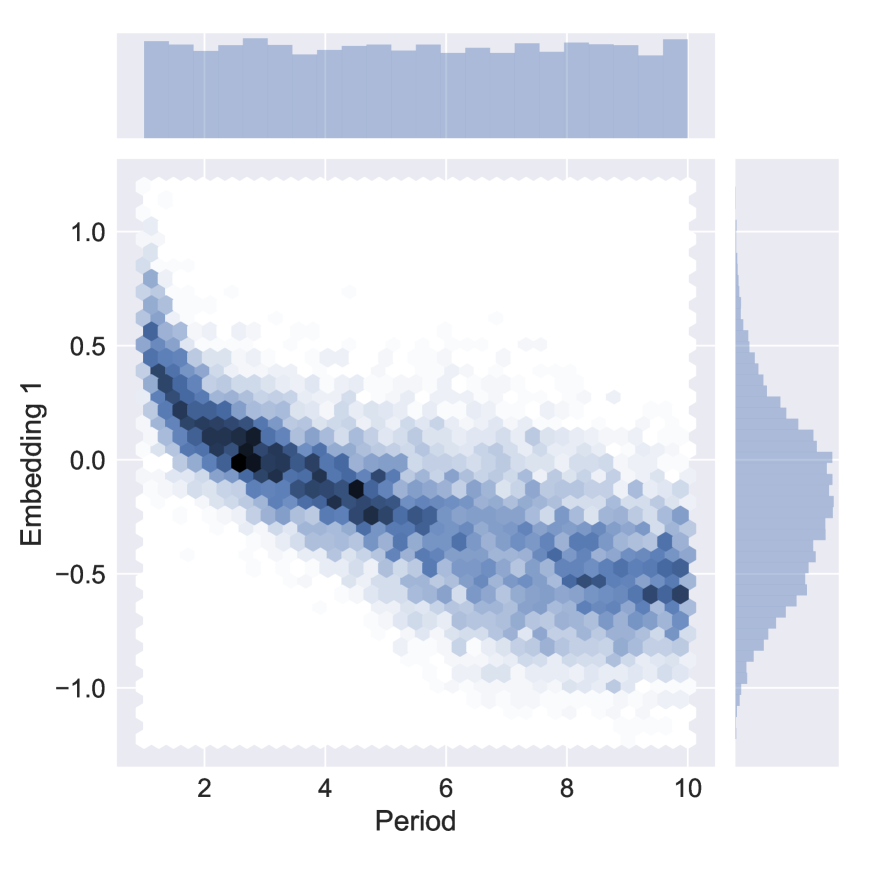
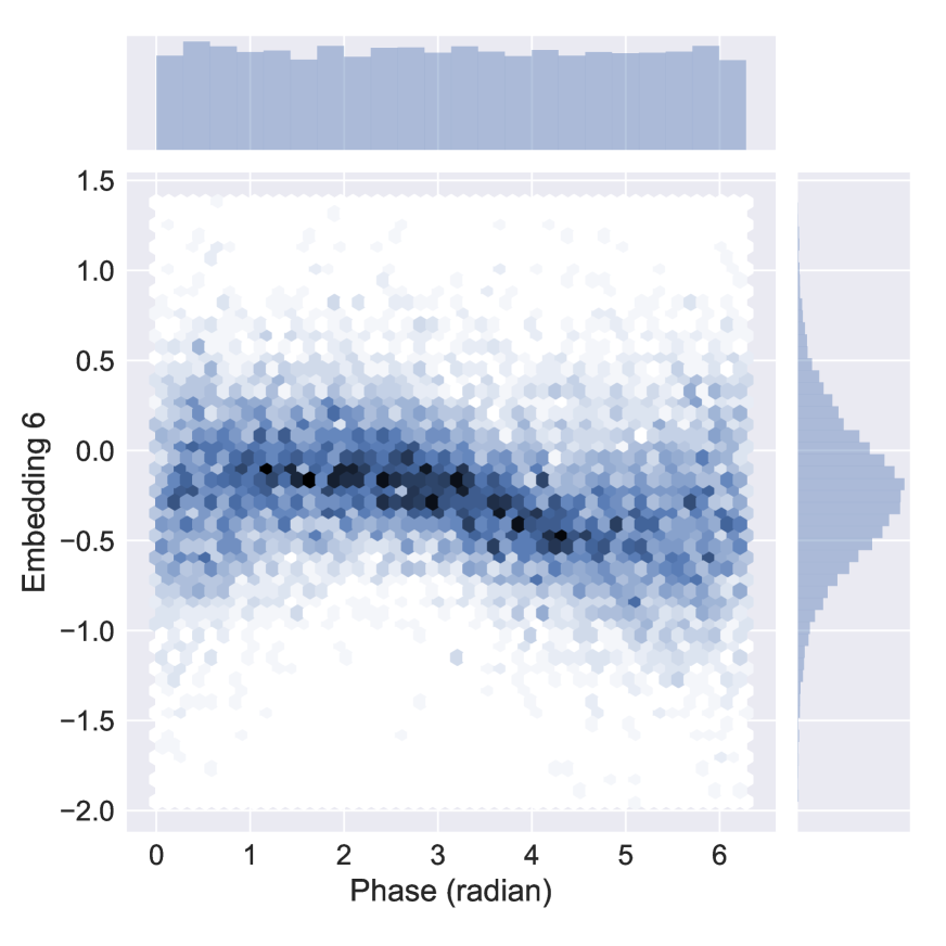
Although the inputs to the autoencoder are only the raw time series measurements and not the periodic parameters, the encoding layer does represents some alternative fixed-dimensional representation of the entire sequence, so it is reasonable to inquire if these values can be used to recover the original parameters $\bm{\theta}_{i}$. Supplementary Figure 9 demonstrates that strong (non-linear) relationships exist between some of the encoding values and the period and phase of the input sequences.

(a) Autoencoder feature vs. period

(b) Autoencoder feature vs. phase

Supplementary Figure 9: Visual depiction of the relationships between 8-dimensional autoencoding time series features and period. We observe clear non-linear relationships between some of the learned autoencoder features and the a) period and b) phase of the input signals. The darkness of each point represents the relative frequency of that region of pairs of values, and the histograms on the top and right show the overall distributions of the estimated parameters and relevant autoencoder features, respectively.

While there is not any obvious closed-form relationship that should exist between a single autoencoding feature and any of the elements of $\bm{\theta}_{i}$, we can attempt to train a separate model mapping the encoding vectors to the parameters of interest. Since the relationships between the autoencoding features appear to be somewhat non-linear, we train a random forest regressor [17] with 1000 trees using cikit-learn ~\cite{pedregoa2011scikit to estimate the period, phase, amplitude, and offset of each sequence using the autoencoding features. 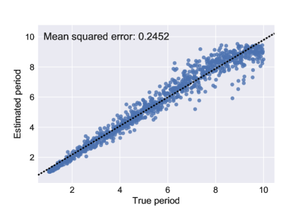Supplementary Figure 10 shows the accuracy of our model for estimating period from the encoding values for various representation lengths; the random forest model is trained on the $N_{\textrm{train}}=50,000$ training sequences and evaluated on the $N_{\textrm{valid}}=10,000$ validation sequences. The accuracy of the model depends on the size of the embedding used, as well as indirectly on many other factors: the size, number, and type of recurrent layers used, the choice of optimization method and stopping criterion, and on the particular distribution chosen for the simulated data. Nevertheless, it is clear from this exercise that useful aggregate properties of time series can be inferred from features automatically generated by an autoencoder. In the next section we explore how these features can be used within the context of a real-world supervised classification problem.

Figure 10: True period vs. estimated period for random forest regressor model. The dotted black line represents an exact math $T_{i}=\hat{T}_{i}$.

4 Application to astronomical light curves of variable stars

4.1 Validation accuracy

The distinction between training, test, and validation data is a subtle one in our problem. In order to avoid overly optimistic results, it is crucial to avoid making use of the test data in any way during the training process. Our experiment, however, is intended to simulate the case where some labeled and some unlabeled light curves are available: in this case, the practitioner is free to train the autoencoder using only the labeled light curves, or using the full dataset. We initially withheld some validation light curves in order to better understand the difference between reconstruction accuracy for light curves that are seen during training versus new light curves; the validation losses reported in Supplementary Figures 11 and 12 are computed using 20% of the available light curves which were withheld during training. After confirming that the reconstruction performance for training and validation light curves was comparable, we re-trained our autoencoder using all the available data before training our random forest classifiers. Supplementary Figure 11 shows the validation loss over time for various embedding sizes. As expected, the embedding size required for an accurate reconstruction is larger than in the case of simulated purely sinusoidal data, and the average reconstruction error at convergence is somewhat higher. Nevertheless, we find that our autoencoder is able to accurately model light curves using a relatively parsimonious feature representation.

(a) By epoch

(b) By time

Figure 11: Comparison of period-folded light curve autoencoder validation losses during training for various embedding sizes. The loss plotted is the mean squared error over the validation set of the reconstructed sequences as a function of a) training epoch and b) training wall time. Each colored line corresponds to a different dimensionality of embedding: for example, “GRU(64) $\times$ 2, Embedding=8” denotes two encoder and two decoder GRU layers each composed of 64 hidden units, with an embedding layer of dimension 8 inbetween.

The above experiments using simulated data show that autoencoders can be used to model periodic sequence that has been irregularly sampled, and that the resulting encodings contain information about the frequency domain properties and other global characteristics of the input time series.

(a) By epoch

(b) By time

Figure 12: Comparison of period-folded light curve autoencoder validation losses during training for various levels of dropout. The loss plotted is the mean squared error over the validation set of the reconstructed sequences as a function of a) training epoch and b) training wall time. Each colored line corresponds to a different dimensionality of embedding: for example, “GRU(64) $\times$ 2, Embedding=8” denotes two encoder and two decoder GRU layers each composed of 64 hidden units, with an embedding layer of dimension 8 inbetween.

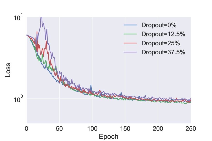
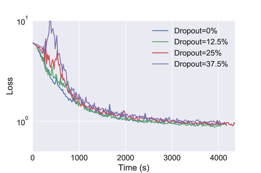
As described in Supplementary Figure 1 of the main text, in our experiments we imposed 25% dropout [14] between recurrent layers in order to avoid overfitting. We tested the effect of dropout using the LINEAR dataset since its smaller size makes overfitting a bigger concern. Supplementary Figure 12 shows how varying the dropout parameter affects the resulting reconstruction validation error; we find that the effect is minimal for this problem.

4.2 Sequence length

As described in the main text, before training our autoencoder we split the available light curves into subsequences of length $n_{T}=200$. This step is purely optional, since our RNN architecture can accommodate input and output sequences of arbitrary length. However, the use of constant-length sequences is advantageous in training: it eliminates the need to pad input sequences and/or mask output sequences when computing the loss function, and empirically it seems to improve training speed (as measured in both iterations and minutes).

(a) By epoch

(b) By time

Figure 13: Comparison of period-folded light curve autoencoder validation losses during training for various sequence lengths. The loss plotted is the mean squared error over the validation set of the reconstructed sequences as a function of a) training epoch and b) training wall time. Each colored line corresponds to a different dimensionality of embedding: for example, “GRU(64) $\times$ 2, Embedding=8” denotes two encoder and two decoder GRU layers each composed of 64 hidden units, with an embedding layer of dimension 8 inbetween.

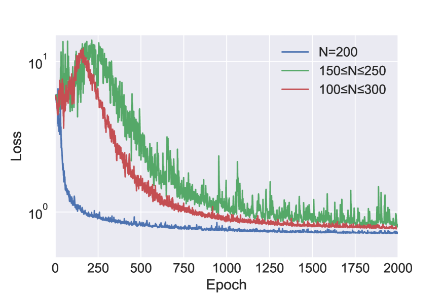
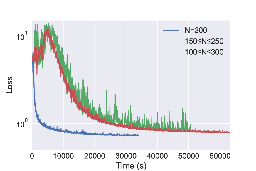
Supplementary Figure 13 depicts the autoencoder training process for different lengths of sequence: first, for constant-size sequences of length $n_{T}=200$; second, for variable-length sequences between $150\leq n_{T}\leq 250$; and finally for $100\leq n_{t}\leq 300$. In each case light curves from the LINEAR dataset were used for training, but for the variable-length sequences the length $n_{T}$ was chosen at random for each light curve subsequence. Although the required training time is significantly longer for the variable-length problem, roughly the same quality of reconstruction is ultimately achieved. However, it is clear that at some point the difference in sequence length would become problematic, and another training approach might need to be explored (for example, grouping different lengths of light curves together and training in batches, or training different models for different sizes of data).

4.3 Data augmentation using noise properties

Data augmentation is commonly applied in the context of image processing tasks in order to increase the effective volumes of available training data (see, e.g., [19]). Unlike in the case of image data, for astronomical surveys the noise properties of the measurements are often known, which provides a natural way to generate synthetic training examples that mimic additional samples from the same survey for a given source. In particular, we attempted to augment our light curve datasets by generating new training samples from existing light curves by adding Gaussian noise corresponding to the estimated measurement error at each time step:

$$\bm{\tilde{}}{y}_{i}=\left(y_{i}^{(1)}+\epsilon_{i}^{(1)},\dots,y_{i}^{(n_{T})}+\epsilon_{i}^{(n_{T})}\right),\ \epsilon_{i}^{(j)}\sim\mathcal{N}(0,\sigma_{i}^{(j)}).$$ (10)

Figure 14: Examples of generated LINEAR light curves using noise properties

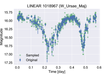
Supplementary Figure 14 depicts three realizations of the light curve resampling process described above. Training our autoencoder on the LINEAR dataset for the same number of epochs but using the additional training samples leads to an increase in validation accuracy from 72.6% to 78.1% for the non-period folded model. However, for the period-folded model, the use of additional training examples did not improve performance, and in fact slightly diminished the validation accuracy (from 97.1% to 96.7%); this is likely because the autoencoder model is already able to accurately reconstruct the period-folded light curves, whereas the raw light curves are not well-modeled and therefore the additional training data is useful. We also attempted applying the same type of noise resampling for the previous example using the ASAS dataset, but the change in accuracy for the resulting classifier was negligible.

4.4 Direct supervised classification

The architecture we have described can easily be modified for other tasks, including direct supervised classification of unevenly sampled time series: in this case, the decoder module in Figure 1 would be replaced by one or more fully-connected layers, and the network would be trained to minimize the multi-class cross entropy classification loss. Such an approach trained on the period-folded data and sampling times also leads to high classification accuracy, achieving 98.6% average validation accuracy for the ASAS dataset and 96.7% for the LINEAR dataset. However, the fully supervised approach requires a large amount of labeled training data, whereas the autoencoder method can make use of either labeled or unlabeled data; the use of unsupervised methods is common in such cases where limited labeled data is available [20].

4.5 Transfer learning

In the experiments in the main text, data from a single survey is used to train an autoencoder, which is then used to produce features used for classification of labeled training examples from the same survey. Because the autoencoder and random forest models are decoupled, it is straightforward to incorporate additional or completely different training data for the unsupervised portion of the model. In the ASAS example, we make use of both labeled and unlabeled examples when training the autoencoder; however, we could just as easily train the autoencoder using only unlabeled data, or data from an entirely different source. As a simple example, we found that features from the autoencoder trained on ASAS or LINEAR data yielded nearly the same level of classification accuracy for light curves from the other survey (less than a 1% reduction in each case).

References

- [1] Levine, A. M. et al. First Results from the All-Sky Monitor on the Rossi X-Ray Timing Explorer. Ap. J. Letters 469, L33 (1996). astro-ph/9608109.
- [2] Pojmanski, G. The all sky automated survey. catalog of variable stars. i. 0 h-6 hquarter of the southern hemisphere. Acta Astronomica 52, 397–427 (2002).
- [3] Murphy, T. et al. VAST: An ASKAP Survey for Variables and Slow Transients. Publications of the Astronomical Society of Australia 30, e006 (2013). 1207.1528.
- [4] Ridgway, S. T., Matheson, T., Mighell, K. J., Olsen, K. A. & Howell, S. B. The Variable Sky of Deep Synoptic Surveys. Astrophysical Journal 796, 53 (2014). 1409.3265.
- [5] Djorgovski, S. et al. Real-time data mining of massive data streams from synoptic sky surveys. Future Gener. Comput. Syst. 59, 95–104 (2016). URL http://dx.doi.org/10.1016/j.future.2015.10.013.
- [6] Kantor, J. Transient Alerts in LSST. In Wozniak, P. R., Graham, M. J., Mahabal, A. A. & Seaman, R. (eds.) The Third Hot-wiring the Transient Universe Workshop, 19–26 (2014).
- [7] Bloom, J. S., Richards, J. W. Data Mining and Machine Learning in Time-Domain Discovery and Classification. In Way, M. J., Scargle, J. D., Ali, K. M. & Srivastava, A. N. (eds.) Advances in Machine Learning and Data Mining for Astronomy, 89–112 (2012).
- [8] Hinton, G. E. & Salakhutdinov, R. R. Reducing the dimensionality of data with neural networks. Science 313, 504–507 (2006).
- [9] Richards, J. W. et al. Construction of a calibrated probabilistic classification catalog: Application to 50k variable sources in the all-sky automated survey. The Astrophysical Journal Supplement Series 203, 32 (2012).
- [10] Breiman, L. Random forests. Machine learning 45, 5–32 (2001).
- [11] Richards, J. W. et al. On machine-learned classification of variable stars with sparse and noisy time-series data. The Astrophysical Journal 733, 10 (2011).
- [12] Naul, B., Van der Walt, S., Crellin-Quick, A., Bloom, J. S. & Pérez, F. cesium: Open-source platform for time-series inference. arXiv preprint arXiv:1609.04504 (2016).
- [13] Nun, I. et al. FATS: Feature Analysis for Time Series. ArXiv e-prints (2015). 1506.00010.
- [14] Dubath, P. et al. Random forest automated supervised classification of Hipparcos periodic variable stars. Monthly Notices of the Royal Astronomical Society 414, 2602–2617 (2011). 1101.2406.
- [15] Nun, I., Pichara, K., Protopapas, P. & Kim, D.-W. Supervised Detection of Anomalous Light Curves in Massive Astronomical Catalogs. Astrophysical Journal 793, 23 (2014). 1404.4888.
- [16] Miller, A. A. et al. A Machine-learning Method to Infer Fundamental Stellar Parameters from Photometric Light Curves. Astrophysical Journal 798, 122 (2015). 1411.1073.
- [17] Kügler, S. D., Gianniotis, N. & Polsterer, K. L. Featureless classification of light curves. Monthly Notices of the Royal Astronomical Society 451, 3385–3392 (2015). 1504.04455.
- [18] Kim, D.-W. & Bailer-Jones, C. A. A package for the automated classification of periodic variable stars. Astronomy & Astrophysics 587, A18 (2016).
- [19] Sesar, B. et al. Exploring the variable sky with linear. ii. halo structure and substructure traced by rr lyrae stars to 30 kpc. The Astronomical Journal 146, 21 (2013).
- [20] Palaversa, L. et al. Exploring the variable sky with linear. iii. classification of periodic light curves. The Astronomical Journal 146, 101 (2013).
- [21] Alcock, C. et al. The macho project lmc variable star inventory. ii. lmc rr lyrae stars-pulsational characteristics and indications of a global youth of the lmc. The Astronomical Journal 111, 1146 (1996).
- [22] Mackenzie, C., Pichara, K. & Protopapas, P. Clustering-based feature learning on variable stars. The Astrophysical Journal 820, 138 (2016).
- [23] Maaten, L. v. d. & Hinton, G. Visualizing data using t-sne. Journal of Machine Learning Research 9, 2579–2605 (2008).
- [24] Cho, K. et al. Learning phrase representations using rnn encoder-decoder for statistical machine translation. arXiv preprint arXiv:1406.1078 (2014).
- [25] Schuster, M. & Paliwal, K. K. Bidirectional recurrent neural networks. IEEE Transactions on Signal Processing 45, 2673–2681 (1997).
- [26] Srivastava, N., Hinton, G. E., Krizhevsky, A., Sutskever, I. & Salakhutdinov, R. Dropout: a simple way to prevent neural networks from overfitting. Journal of Machine Learning Research 15, 1929–1958 (2014).
Acknowledgements
We would thank Yann LeCun and Farid El Gabaly for helpful discussions, and Aaron Culich for computational assistance. This work is supported by the Gordon and Betty Moore Foundation Data-Driven Discovery and NSF BIGDATA Grant #1251274. Computation was provided by the Pacific Research Platform program through NSF ACI #1541349, OCI #1246396, UCOP, Calit2, and BRC at UC Berkeley.
- [1]
- [2] Charnock, T. & Moss, A. Deep recurrent neural networks for supernovae classification. arXiv preprint arXiv:1606.07442 (2016).
- [3] Che, Z., Purushotham, S., Cho, K., Sontag, D. & Liu, Y. Recurrent neural networks for multivariate time series with missing values. arXiv preprint arXiv:1606.01865 (2016).
- [4] Lipton, Z. C., Kale, D. C., Elkan, C. & Wetzell, R. Learning to diagnose with lstm recurrent neural networks. arXiv preprint arXiv:1511.03677 (2015).
- [5] Friedman, J. H. & Silverman, B. W. Flexible parsimonious smoothing and additive modeling. Technometrics 31, 3–21 (1989).
- [1] Lapedes, A. & Farber, R. Nonlinear signal processing using neural networks: prediction and system modeling. Los Alamos National Laboratory Technical Report LA-UR-87-2662 (1987).
- [2] LeCun, Y., Bengio, Y. et al. Convolutional networks for images, speech, and time series. The handbook of brain theory and neural networks 3361, 1995 (1995).
- [3] Hinton, G. et al. Deep neural networks for acoustic modeling in speech recognition: The shared views of four research groups. IEEE Signal Processing Magazine 29, 82–97 (2012).
- [4] Pascanu, R., Mikolov, T. & Bengio, Y. On the difficulty of training recurrent neural networks. ICML (3) 28, 1310–1318 (2013).
- [5] Hochreiter, S. & Schmidhuber, J. Long short-term memory. Neural computation 9, 1735–1780 (1997).
- [6] Cho, K. et al. Learning phrase representations using rnn encoder-decoder for statistical machine translation. arXiv preprint arXiv:1406.1078 (2014).
- [7] Graves, A., Mohamed, A.-r. & Hinton, G. Speech recognition with deep recurrent neural networks. In Acoustics, speech and signal processing (icassp), 2013 ieee international conference on, 6645–6649 (IEEE, 2013).
- [8] Bahdanau, D., Cho, K. & Bengio, Y. Neural machine translation by jointly learning to align and translate. arXiv preprint arXiv:1409.0473 (2014).
- [9] Mikolov, T., Karafiát, M., Burget, L., Cernockỳ, J. & Khudanpur, S. Recurrent neural network based language model. In Interspeech, vol. 2, 3 (2010).
- [10] Beylkin, G. On the fast fourier transform of functions with singularities. Applied and Computational Harmonic Analysis 2, 363–381 (1995).
- [11] Lomb, N. R. Least-squares frequency analysis of unequally spaced data. Astrophysics and space science 39, 447–462 (1976).
- [12] Scargle, J. D. Studies in astronomical time series analysis. ii-statistical aspects of spectral analysis of unevenly spaced data. The Astrophysical Journal 263, 835–853 (1982).
- [13] Kingma, D. & Adam, J. B. A method for stochastic optimization. arXiv preprint arXiv:1412.6980 (2014).
- [14] Srivastava, N., Hinton, G. E., Krizhevsky, A., Sutskever, I. & Salakhutdinov, R. Dropout: a simple way to prevent neural networks from overfitting. Journal of Machine Learning Research 15, 1929–1958 (2014).
- [15] Chollet, F. Keras. https://github.com/fchollet/keras (2015).
- [16] Schwarzenberg-Czerny, A. Accuracy of period determination. Monthly Notices of the Royal Astronomical Society 253, 198–206 (1991).
- [17] Breiman, L. Random forests. Machine learning 45, 5–32 (2001).
- [18] Pedregosa, F. et al. Scikit-learn: Machine learning in python. Journal of Machine Learning Research 12, 2825–2830 (2011).
- [19] Simard, P. Y., Steinkraus, D., Platt, J. C. et al. Best practices for convolutional neural networks applied to visual document analysis. In ICDAR, vol. 3, 958–962 (2003).
- [20] Glorot, X., Bordes, A. & Bengio, Y. Domain adaptation for large-scale sentiment classification: A deep learning approach. In Proceedings of the 28th international conference on machine learning (ICML-11), 513–520 (2011).