Tensor Modes in Pure Natural Inflation

Abstract

We study tensor modes in pure natural inflation Nomura:2017ehb , a recently-proposed inflationary model in which an axionic inflaton couples to pure Yang-Mills gauge fields. We find that the tensor-to-scalar ratio $r$ is naturally bounded from below. This bound originates from the finiteness of the number of metastable branches of vacua in pure Yang-Mills theories. Details of the model can be probed by future cosmic microwave background experiments and improved lattice gauge theory calculations of the $\theta$-angle dependence of the vacuum energy.

Cosmic inflation is a successful framework in explaining many distinguished features of our Universe, including its flatness and the origin of primordial density perturbations. There are, however, a plethora of inflationary models proposed in the literature, and we ultimately need to turn to observations for guidance, to convincingly answer the question of exactly which inflationary model describes our Universe.

Future detection of primordial tensor modes in comic microwave background (CMB) radiation would be ideal for this purpose. The size of primordial tensor modes is quantified by the tensor-to-scalar ratio $r$, and when combined with the observed value of the scalar spectral index $n_{s}$, these two parameters severely constrain models of inflation. This therefore provides an exciting opportunity for narrowing down possible models, especially because values of $r\sim 10^{-3}$ are expected to be within reach in next-generation CMB measurements (see e.g. Ref. Creminelli:2015oda ).

The goal of this paper is to study the prediction for tensor modes of the recently-proposed inflationary model of pure natural inflation Nomura:2017ehb . This is arguably the simplest model of inflation consistent with the current observational data. It is defined within conventional low-energy effective field theory and is technically natural, i.e. stable under quantum corrections.

The model is given by an axionic inflaton $\phi$ coupling to four-dimensional pure Yang-Mills gauge fields:

$$\mathcal{L}_{\phi FF}=\frac{1}{32\pi^{2}}\frac{\phi}{f}\epsilon^{\mu\nu\rho\sigma}\textrm{Tr}F_{\mu\nu}F_{\rho\sigma},$$ (1)

where $f$ is the decay constant and the dimensionless combination $\theta:=\phi/f$ plays the role of the $\theta$-angle of the Yang-Mills theory. Below we choose the Yang-Mills gauge group to be $SU(N)$ for simplicity.

The inflaton potential $V(\phi)$ is determined by the dynamics of the pure Yang-Mills theory. For our purposes, it is useful to parameterize the potential in the form

$$V(\phi)=M^{4}\left[1-\frac{1}{\left(1+(\phi/F)^{2}\right)^{p}}\right].$$ (2)

Here, $M$ and $F$ are two parameters which have dimensions of mass, and the exponent $p>0$ is a dimensionless parameter. The parameter $F$ plays the role of the effective decay constant.

This potential is motivated by the holographic computation of Ref. Dubovsky:2011tu , which gives the parameters $M$ and $F$ to be

$$M\approx\sqrt{N}\Lambda,\qquad F\approx Nf,$$ (3)

where $\Lambda$ is the dynamical scale of the Yang-Mills theory. We define the parameter $\gamma$ by

$$F=\pi\gamma Nf.$$ (4)

As we will see later, $\gamma\approx O(1)$. For our purposes, we use $\gamma$ and the power $p$ to parameterize the strong-coupling dynamics of the Yang-Mills theory.

The potential of Eq. (2) takes approximately the quadratic form $V(\phi)\sim\phi^{2}$ for $\phi\ll F$, but it begins to deviate from this form as $\phi/F$ becomes larger. Note that this potential is rather different from the cosine potential used in the original model of natural inflation Freese:1990rb ; Adams:1992bn , which is motivated by the instanton approximation—as explained in Ref. Nomura:2017ehb , the cosine potential is not theoretically valid for pure Yang-Mills theory, and is also disfavored by the recent observations by Planck Ade:2015lrj and BICEP2/Keck Array Array:2015xqh .

The parameter $M$ in Eq. (2) is determined by the overall size of the scalar perturbation once the other parameters, $F$ and $p$, are given. While the power spectrum depends on all these parameters, in the range of $F$ and $p$ considered in this paper, we find

$$M\sim 10^{16}~{}{\rm GeV}.$$ (5)

This implies that to discuss the tensor-to-scalar ratio $r$ and spectral index $n_{s}$, only the effective decay constant $F$ and the power $p$ are relevant. When we vary these parameters, we obtain a range of $r$ and $n_{s}$ which are in impressive agreement with the current observational constraints; see Fig. 1.

Figure 1: The values of $n_{s}$ and $r$ predicted by the model for the number of e-folds $N_{e}=50,60$ and for $p=1,2,3,4,6$. The light (dark) blue region represents the 95% (68 %) CL allowed region by Planck Ade:2015lrj and BICEP2/Keck Array Array:2015xqh . $F/M_{\rm Pl}=10,5,1$ are indicated by dots (from top to bottom). This plot is the same as that in Fig. 3 of Ref. Nomura:2017ehb , except for the choice of the values of $p$.

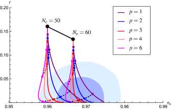
We see that the value of the spectral index $n_{s}$ is mostly consistent with observation regardless of the values of $F$ and $p$. On the other hand, the size of the tensor-to-scalar ratio $r$ strongly depends on the value of $F$. Our main interest in this paper is to figure out the expected size of the tensor-to-scalar ratio $r$, or equivalently the value of $F$, in the present model.

If $F$ is large, $F\gtrsim M_{\rm Pl}$, we expect to have a large value of $r$, and hence tensor modes can be observationally found in the near future. Here, $M_{\rm Pl}\simeq 1.22\times 10^{19}~{}{\rm GeV}$ is the Planck scale. In the limit that $F$ is very large, $F\gg M_{\rm Pl}$, the prediction of the model approaches that of chaotic inflation Linde:1983gd with the quadratic potential $V(\phi)=m^{2}\phi^{2}/2$, which is now excluded at about a $3\sigma$ level Ade:2015lrj ; Array:2015xqh . However, as discussed in our previous paper Nomura:2017ehb , this extreme limit is not available in our framework, since the validity of low-energy effective field theory puts a constraint $F\lesssim O(M_{\rm Pl})$.

In the opposite limit of small $F$, the tensor-to-scalar ratio $r$ is small; in fact, it can be tiny if $F$ is much smaller than $M_{\rm Pl}$. At first sight, there seems to be no issue in going to this extreme parameter region. The predicted value of $n_{s}$ is consistent with current experimental bounds, as can be seen in Fig. 1. The necessary amount of inflation, $N_{e}\approx 50\mbox{--}60$, can be obtained if the initial value of the inflaton field is large, $\phi\gg F$. However, there is a reason to think that such a parameter region may not be available in the model. This has to do with the fact that the potential in Eq. (2) is motivated by the holographic computation in the large $N$ limit, and it should not be taken at face value once we taken into account the finite $N$ effects.

To explain this point (in the language of quantum field theory), let us first recall the salient features of the large $N$ analysis Witten:1979vv ; Witten:1980sp .

In addition to the axion coupling in Eq. (1), we have the kinetic term for the gauge fields, so that the total Lagrangian density is given by

$$\mathcal{L}=N\left[-\frac{1}{4\lambda}\textrm{Tr}(F^{\mu\nu}F_{\mu\nu})+\frac{1}{32\pi^{2}}\frac{\phi}{Nf}\epsilon^{\mu\nu\rho\sigma}\textrm{Tr}F_{\mu\nu}F_{\rho\sigma}\right].$$ (6)

Here, we have factored out the overall coefficient $N$, and $\lambda=g^{2}N$ is the ’t Hooft coupling with $g$ being the gauge coupling. In the large $N$ limit tHooft:1973alw , the parameter $1/N$ plays the role of an expansion parameter. Physical observables are expected to be smooth functions of $\lambda$ and $\phi/(Nf)$, which are kept finite in taking the limit.

From this large $N$ scaling argument, we expect that the potential of $\phi$, i.e. the $\theta$-angle dependence of the vacuum energy, takes the form

$$V(\phi)=N^{2}\Lambda^{4}\mathsf{V}\left(\frac{\phi}{Nf}\right)+O(N^{0}),$$ (7)

where $\mathsf{V}(x)$ is a smooth function of $O(N^{0})$ when written in terms of $x$. This potential, however, does not respect the expected symmetry under $\phi\to\phi+2\pi f$. In the large $N$ limit, this transformation induces an infinitesimal shift in the argument of function $\mathsf{V}$, which can be an invariance of the potential $V(\phi)$ only if $\mathsf{V}$ is constant. However, this is inconsistent with perturbative large $N$ calculation, which shows otherwise.

The way around this problem is to realize that the potential is multi-valued Witten:1980sp . In particular, we have many different (in general metastable) branches corresponding to the shift $\phi\to 2\pi fn$ with $n$ integer. The correct vacuum energy, for example, is then given by the minimal values among these branches

$$V_{\rm min}(\phi)=N^{2}\Lambda^{4}\textrm{min}_{n}\mathsf{V}\left(\frac{\phi+2\pi fn}{Nf}\right),$$ (8)

so that the invariance of physics under $\phi\to\phi+2\pi f$ is recovered.

Let us now come to finite values of $N$. In the large $N$ analysis the value of $N$ is taken to be infinity, so that we have an infinitely many branches, i.e. $n$ runs over all integers in Eq. (8). However, the situation can be different for a finite value of $N$—if $n$ is taken to be of order $N$ then the shift $\phi\to\phi+2\pi fn$ changes the argument of $\mathsf{V}(\phi/(Nf))$ by an $O(1)$ amount, which can preserve the value of the function $\mathsf{V}(\phi/(Nf))$. If this happens, there will be only a finite number of metastable branches, with each branch being periodic with the period of $O(2\pi Nf)$.

That a finite number (order $O(N)$) of branches exists is discussed in the analysis of the chiral Lagrangian for QCD (with flavors) in Ref. Witten:1980sp . The analysis there is justified for small quark masses, whereas here we are interested in the opposite limit of pure Yang-Mills theory, in which the quark masses are taken to be infinitely large.

In the case of pure Yang-Mills theory, we expect that the number of metastable branches is $N$ (so that the periodicity of the $\theta$-dependent potential in a single branch is $2\pi N$, not $2\pi$). This is suggested for example by the analysis of softly-broken $\mathcal{N}=1$ supersymmetric Yang-Mills theories (see Refs. Dine:2014hwa ; Yonekura:2014oja ). More recently, this $2\pi N$ periodicity of the $\theta$ angle has been made manifest when we turn on the background gauge fields for the center of the gauge group Gaiotto:2017yup .

Yet another support comes from the recent work of Ref. Yamazaki:2017ulc (see also Yamazaki:2017dra ), which has given a concrete argument that the number of branches is $N$ (so that we have $\mathsf{V}(x+2\pi)=\mathsf{V}(x)$). This paper studied a compactification of pure $SU(N)$ Yang-Mills theory on $\mathbb{R}\times\mathbb{T}^{3}$, twisted by the $\mathbb{Z}_{N}$ center symmetry. There the $\theta$ angle of the Yang-Mills theory is identified with the $\theta$ angle of the $\mathbb{CP}^{N-1}$ model, where $\mathbb{CP}^{N-1}$ arises as the moduli space of flat connections on $\mathbb{T}^{2}$. The classical vacua of the theory are given by the $N$ fixed points of the twisted boundary condition of the $\mathbb{CP}^{N-1}$ model, thereby identifying the $N$ vacua explicitly in a weakly coupled region.

Given all the evidence, we assume below that the number of different branches is $N$:

$$V(\phi+2\pi Nf)=V(\phi).$$ (9)

In addition, we have parity symmetry $V(\phi)=V(-\phi)$ and know the form of the potential near the origin, $\mathsf{V}(x)\sim x^{2}$ from perturbative large $N$ calculation. These imply that the potential should have a plateau region of finite size around $\phi\sim\pi Nf$; see Fig. 2. Here and below, we focus on the branch that has a minimum at $\phi=0$ without loss of generality.

Figure 2: A sketch of the inflaton potential $V(\phi)$ for a finite value of the gauge group rank $N$. We show the branch structure corresponding to the shift of $\phi$ by $2\pi nf$ ($n=1,2,\ldots$) with different colors. Each metastable branch has a period of $2\pi Nf$ to account for the $N$-fold degeneracy of metastable vacua. We have a plateau near the value $\phi\sim\pi NF$ (for a branch that has a minimum at $\phi=0$), which however has only a finite width for consistency with the $2\pi Nf$ periodicity.

An important point is that the plateau portion of the potential, which is useful for inflation, cannot continue indefinitely, since the potential decreases as $\phi$ deviates far from a minimum, e.g. in the region $N\pi f<|\phi|<2N\pi f$ when viewed from $\phi=0$. This implies that the value of the inflaton corresponding to the current horizon scale, which we denote by $\phi_{*}$, can be restricted to the region $\phi_{*}\in[0,N\pi f]$ without loss of generality. (If the initial value of the inflaton $\phi_{i}$ is larger than $N\pi f$, then the inflaton will roll into another minimal $2N\pi f$, resulting in the identical physics as the inflaton starting from $2\pi f-\phi_{i}$.) Note that we do not know the precise form of the potential around the turning point $\phi\sim N\pi f$. However, the potential of Eq. (2) is already quite flat around these points, and we expect that it smoothly connects to the $2N\pi$ shifted potential, as depicted in Fig. 2.

Let us define the variable

$$y\equiv\frac{\phi_{*}}{F}.$$ (10)

Since $y\approx\phi_{*}/N\pi f$ (see Eq. (4)), the parameter space for this quantity is bounded

$$y\leq\frac{1}{\gamma}\equiv y_{\rm max}\approx O(1),$$ (11)

where $y=y_{\rm max}$ corresponds to $\phi_{*}=N\pi f$; see Fig. 2. In this paper, we do not consider the case in which $y$ is extremely close to $y_{\rm max}$, i.e. the case in which observable inflation starts near $\phi=N\pi f$.

There are several reasons for this. First, for $\phi$ very close to $N\pi f$, we cannot trust the form of the potential in Eq. (2). In this region, the potential becomes flat, with $dV(\phi)/d\phi=0$ at $\phi=N\pi f$. Since the potentials of many branches are almost degenerate there, we suspect that tunnelings between different branches may not be negligible. Furthermore, one might argue that natural values for $y$ are not close to $y_{\rm max}$. Since the axion is a pseudo Nambu-Goldstone boson, the inflaton potential is regarded as a flat direction at energy scales much larger than $M$. One may then expect that the initial value of the inflaton $\phi_{i}$ is distributed uniformly in the interval $[0,N\pi f]$. If this is the case, then we expect

$$y\lesssim 0.5y_{\rm max},$$ (12)

“on average.” Below, we consider that

$$y\lesssim 0.9y_{\rm max}.$$ (13)

We assume that in this parameter region, the potential of Eq. (2) can be used to predict $n_{s}$ and $r$.

The prediction for $r$ depends somewhat sensitively on $y_{\rm max}$, i.e. the value of $\gamma$ in Eq. (4). This parameter, however, can be determined from first-principle computations in lattice gauge theory.

To see this, let us expand the potential in power series in $\theta=\phi/f$:

$$V(\theta)=\frac{1}{2}\chi\theta^{2}\left(1+\sum_{n=1}^{\infty}b_{2n}\theta^{2n}\right),$$ (14)

where the leading coefficient $\chi$ is known as the topological susceptibility, and the sub-leading coefficients have the large $N$ expansion Witten:1980sp

$$b_{2n}=\frac{\bar{b}_{2n}}{N^{2n}}\left(1+O\left(\frac{1}{N^{2}}\right)\right).$$ (15)

The potential of Eq. (2) gives values

$$\bar{b}_{2}=-\frac{p+1}{2}\left(\frac{1}{\pi\gamma}\right)^{2},\quad\bar{b}_{4}=\frac{(p+1)(p+2)}{6}\left(\frac{1}{\pi\gamma}\right)^{4}.$$ (16)

This should be compared with the recent results from lattice gauge theory Bonati:2016tvi

$$\bar{b}_{2}=-0.23(3),\quad\bar{b}_{4}\lesssim 0.1.$$ (17)

From this, $\gamma$ is determined in terms of $p$ as

$$\gamma\simeq 0.47\sqrt{p+1},$$ (18)

giving rise to the constraint

$$y\lesssim 0.9\frac{2.1}{\sqrt{p+1}}\simeq\frac{1.9}{\sqrt{p+1}}.$$ (19)

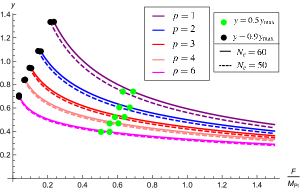
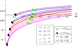
This constraint can be translated into a lower bound on the effective decay constant $F$, and then into a lower bound on the tensor-to-scalar ratio $r$. In Fig. 3, we plot the value of $y$ as a function of $F/M_{\rm Pl}$ for $p=1,2,3,4,6$, assuming that the number of e-folds for observation inflation (inflation occurring in $\phi\leq\phi_{*}$) is $N_{e}=50,60$. The black and green dots correspond to $y=0.9y_{\rm max}$ and $0.5y_{\rm max}$, respectively. We find that with $y<0.9y_{\rm max}$, $F$ is bounded from below. In Fig. 4, we give a similar plot, but now the vertical axis is $r$. We find that the value of $r$ is bounded from below.

Figure 3: The value of $y=\phi_{*}/F$ as a function of $F/M_{\rm Pl}$ for $N_{e}=60$ (solid) and $50$ (dashed) for $p=1,2,3,4,6$ (from top to bottom). Here, $\phi_{*}$ is the value of the inflaton at which observable inflation starts (i.e. inflation occurring in the region $\phi\leq\phi_{*}$ has $N_{e}$ e-folds). Black dots represent $y=0.9y_{\rm max}$ with $y_{\rm max}=2.1$; see Eq. (19). Green dots represent $y=0.5y_{\rm max}$.

Figure 4: The tensor-to-scalar ratio $r$ as a function of $F/M_{\rm Pl}$ for $N_{e}=60,50$ for $p=1,2,3,4,6$. Lines and dots are the same as in Fig. 3.

Figure 5: Predictions of the model on the $n_{s}$-$r$ plane. Lines and dots are the same as in Fig. 3; in particular, black (green) dots represent the bound $y<0.9y_{\rm max}$ ($0.5y_{\rm max}$). The light (dark) blue region represents the allowed parameter region under the 95% (68%) CL from Planck Ade:2015lrj and BICEP2/Keck Array Array:2015xqh .

Figure 6: The same as in Fig. 5 but zoomed into the region of small $r$, which is now plotted in a logarithmic scale.

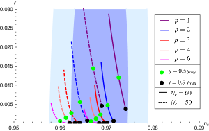
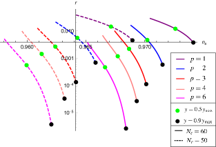
In Figs. 5 and 6, we plot the points $y=0.9y_{\rm max}$ and $0.5y_{\rm max}$ on the standard $n_{s}$-$r$ plane. We find that predictions for $n_{s}$ are consistent with the current data, although its detailed values depend on $N_{e}$ and $p$. On the other hand, the prediction for $r$ depends rather sensitively on $y$, i.e. $F$, and $p$. For $N_{e}=60$, for example, we obtain

$$r\gtrsim\left\{\begin{array}[]{ll}3.8\times 10^{-3}&(p=1),\\ 1.1\times 10^{-4}&(p=3),\\ 2.7\times 10^{-6}&(p=6),\end{array}\right.$$ (20)

for $y<0.9y_{\rm max}$, with

$$r\simeq\left\{\begin{array}[]{ll}1.2\times 10^{-2}&(p=1),\\ 2.2\times 10^{-3}&(p=3),\\ 4.7\times 10^{-4}&(p=6),\end{array}\right.$$ (21)

for $y=0.5y_{\rm max}$. These values of $r$ are interesting because a significant portion of the parameter space can be probed by next-generation CMB measurements, which are expected to reach $r\sim 10^{-3}$. With an improved measurement of $n_{s}$, this would allow us to probe the model further, especially if the value of $p$ is small.

At this point, the power $p$ is unknown. However, it may be determined/constrained if the lattice gauge theory computation of $b_{4}$ is improved by one order of magnitude or more. The power $p$ is given by the ratio between $\bar{b}_{4}$ and $\bar{b}_{2}^{2}$ as

$$\bar{b}_{4}=\frac{2(p+2)}{3(p+1)}\bar{b}_{2}^{2}\simeq\frac{p+2}{p+1}\times 3.5\times 10^{-2}.$$ (22)

For relatively small $p$, this relation may be used to determine its value. It may indeed be possible to test the model through an interplay between future cosmological observations and lattice gauge theory computations.

In conclusion, we have studied predictions for tensor modes in pure natural inflation. We have found that the tensor-to-scalar ratio $r$ is bounded from below under natural assumptions. This originates from the fact that the number of metastable branches for $SU(N)$ gauge theory is $N$ (a finite value), and hence the field space for inflaton is limited. The actual bound depends on features of the inflaton potential that cannot be computed analytically. The parameter region of the model, however, will be constrained by future improvements of lattice gauge theory calculations and future observations of CMB radiation. It is interesting that physics of strongly coupled gauge theories has direct implications for both theory and observations of early universe cosmology.