Minimisation strategies for the determination of parton density functions

Abstract

We discuss the current minimisation strategies adopted by research projects involving the determination of parton distribution functions (PDFs) and fragmentation functions (FFs) through the training of neural networks. We present a short overview of a proton PDF determination obtained using the covariance matrix adaptation evolution strategy (CMA-ES) optimisation algorithm. We perform comparisons between the CMA-ES and the standard nodal genetic algorithm (NGA) adopted by the NNPDF collaboration.

1 Introduction

In perturbative QCD, parton distribution functions are used to describe the nonperturbative structure of hadrons. These functions are typically determined by means of a fit to a wide set of experimental data [1]. Such a fit is complicated by the non-trivial relationship between parton distributions and physical observables. Data on hadron-hadron collider processes is related to parton distributions by means of a double convolution with a kernel computed in perturbation theory. Given some representation of PDFs: $f$ in terms of a set of model parameters: $\{a\}$ a typical hadron-hadron collider observable $T$ may be be calculated as

$$T[f\{a\}]=\int{\widetilde{T}_{ij}(x_{1},x_{2})f_{i/1}(x_{1},\{a\})f_{j/2}(x_{2},\{a\}),}$$ (1)

where $f_{i/1}$ and $f_{j/2}$ represent the parton distributions for PDF flavours $i/j$ of the first and second beams respectively, and $\widetilde{T}$ is the relevant integration kernel for the observable $T$. The model parameters may then be determined by a fit to data by minimising some figure of merit, for example the correlated $\chi^{2}$ between theory and data

$$\chi^{2}(\{a\})=\sum_{i,j}^{N_{\rm dat}}(T_{i}[f]-D_{i})(C_{ij})^{-1}(T_{j}[f]-D_{j})\,\mbox{,}$$ (2)

where $D_{i}$ represents the $i^{\mathrm{th}}$ data point in a set with covariance $C$. For the most part, in PDF determinations this minimisation procedure is performed with the use of standard gradient descent methods. However the computation of the fitness gradient with respect to model parameters, i.e.

$$\frac{\partial\chi^{2}}{\partial a},$$ (3)

is challenging due to the relationship between theory predictions and PDFs expressed in Equation 1. For fits of PDF models with relatively few parameters, such gradients may be either directly computed or reasonably approximated by the equivalent finite-differences. However when using models with a relatively large parameter space, such as those used in determinations in the NNPDF approach, the computation or approximation of these gradients can be a considerable computational burden. Consequently in NNPDF determinations of parton distributions, gradient-free minimisation methods have been employed. These typically take the form of a Nodal Genetic Algorithm (NGA) variant [2]. At each iteration of the minimisation, candidate parameter values are sampled around a search centre according to a Gaussian distribution, with the candidate minimising the $\chi^{2}$ being selected for the search centre in the next iteration. Such an algorithm is greedy in that it always makes the locally optimal selection for the next iteration. For details of the algorithm see Ref. [3].

Despite the simplicity of the algorithm, it has proven to be an efficient way of exploring the complicated PDF parameter space in a manner that is relatively robust in terms of avoiding features such as local minima. However there are clear directions for improvement in terms of a minimisation algorithm. Firstly, the algorithm does not make use of any information on the structure of the parameter space in order to guide the exploration in subsequent steps. Secondly the current algorithm is rather sensitive to noise in the objective function, as it is constrained to only select the locally best candidate at each iteration.

In the NNPDF approach, the inherent susceptibility of the minimisation algorithm to noise is ameliorated by two mechanisms. Each PDF determination is performed as an ensemble of fits to different sub-samples of the complete dataset. This ensemble determination reduces the sensitivity of the overall result to fluctuations affecting individual fits, however there is the potential for PDF uncertainties to be inflated due to overly noisy ensemble members. Furthermore a form of cross-validated early stopping is applied to avoid over-fitting. This does not however completely prevent contamination of the results by noise.

In a recent application of the NNPDF methodology to the determination of fragmentation functions [4] an alternative minimisation strategy was employed, the active $(\mu,\lambda)$-CMA-ES algorithm [5, 6]. The CMA-ES procedure includes mechanisms which overcome the two weaknesses in the standard NNPDF NGA minimisation described above. In the application to fragmentation functions, CMA-ES proved a reliable and efficient minimisation algorithm. Here we shall report results from a preliminary investigation into the application of the algorithm in the case of proton PDFs.

2 Comparison of minimisers

Two fits have been performed at NNLO in the NNPDF3.1 framework [7], one utilising the NGA minimiser, and the second with the CMA-ES algorithm with population $\mu=80$ and initial step-size $\sigma=0.1$. All other CMA-ES parameters are set as per the recommended defaults. The dataset and other fit parameters are identical to those used in the NNPDF3.1 NNLO determination.

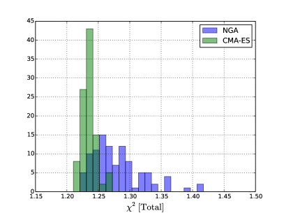
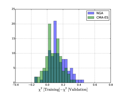
In the first panel of Figure 1 we show the distribution of $\chi^{2}$ fitness over the two PDF ensembles. The total $\chi^{2}$ distribution demonstrates a significant difference between the results from the two minimisers. Ensemble members of the CMA-ES fit are typically better fit to their datasets than the NGA equivalent. Furthermore the results from the CMA-ES fit are considerably more consistent between ensemble members. To verify that this improvement in total fitness is not due to over-learning the training dataset, in the second panel we histogram the differences between the $\chi^{2}$ to the datasets used for training and validation. While results here are more consistent between the two minimisers, it is clear that the CMA-ES results have a slightly better balance between the training and validation fitnesses than in the NGA equivalent.

Figure 1: Histogram of $\chi^{2}$ fitness to the total dataset (left) and the difference between training and validation $\chi^{2}$ (right). Shown are the fitnesses of the CMA-ES ensemble (blue) and the NNPDF ensemble (green).

To investigate the greater ensemble consistency demonstrated in the CMA-ES $\chi^{2}$ distribution, the arc-length defined as

$$L=\int{\sqrt{1+\left(\frac{df}{dx}\right)^{2}}dx,}$$ (4)

is a useful quantity in that it offers a measure of the structural ‘complexity’ of a function. For a fit determining an underlying function that is expected to be largely smooth, results from fits suffering from contamination by noise in the objective function would be expected to have a typically larger arc-length than those less susceptible to noise.

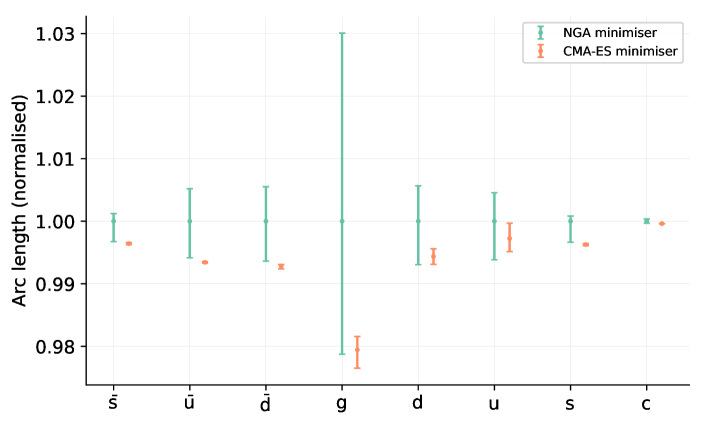
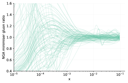
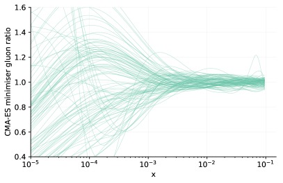
In Figure 2 we compare the arc-lengths of the PDFs determined by the NGA minimiser and the CMA-ES . The figure demonstrates a clear and significant difference in both the PDF arc-lengths and their spread over the fit ensemble. The CMA-ES results demonstrate consistently lower and more regular arc-lengths, confirming the expectation that the results from the CMA-ES should be more resistant to noise in the objective function. Particularly striking is the difference in arc-length for the gluon PDF . A direct comparison of the gluon determination in the CMA-ES and NGA minimisers is shown in Figure 3, where even though the results are consistent between the two minimisers, the reduced structural complexity of the CMA-ES result can be clearly seen.

Figure 2: Arc-lengths $L$ for PDFs determined via the NGA and CMA-ES minimisers . Results are normalised to the NGA value, and uncertainties are given as asymmetric 68% confidence intervals.

Figure 3: Gluon PDF ensemble distributions for the NGA (left) and the CMA-ES (right) minimisers. Each distribution is normalised to its central-value.

3 Conclusion

The CMA-ES minimiser has been successfully applied to the determination of parton distribution functions in the NNPDF approach. Results determined through the CMA-ES procedure exhibit greater consistency, improved agreement with data, and reduced complexity in comparison to results determined through the NGA minimiser. While these improvements are clear from performing fits to real data, the statistical consistency of the results are yet to be established. In terms of arc-lengths, while lower structural complexity may indicate a reduced sensitivity to noise in the objective function, it may also indicate an overly restrictive minimisation procedure whereby uncertainties may be underestimated. In order to ensure the statistical consistency of the results, further tests are needed. In Ref. [3] the consistency of the PDF uncertainties were determined by means of statistical closure tests. For the minimiser investigated here to provide reliable fits of PDFs, it must be able to demonstrate closure on a pseudo-dataset. These tests we leave for a future work.

References

- [1] J. Gao, L. Harland-Lang and J. Rojo, “The Structure of the Proton in the LHC Precision Era,” arXiv:1709.04922 [hep-ph].
- [2] D. J. Montana and L. Davis, Training Feedforward Neural Networks Using Genetic Algorithms, in Proceedings of the 11th International Joint Conference on Artificial Intelligence - Volume 1, IJCAI’89, (San Francisco, CA, USA), pp. 762–767, Morgan Kaufmann Publishers Inc., 1989.
- [3] R. D. Ball et al. [NNPDF Collaboration], JHEP 1504 (2015) 040 doi:10.1007/JHEP04(2015)040 [arXiv:1410.8849 [hep-ph]].
- [4] V. Bertone et al. [NNPDF Collaboration], Eur. Phys. J. C 77 (2017) no.8, 516 doi:10.1140/epjc/s10052-017-5088-y [arXiv:1706.07049 [hep-ph]].
- [5] N. Hansen, A. Ostermeier, “Completely derandomized self-adaptation in evolution strategies,” Evolutionary Computation (2001), no.2, 159-195 doi:10.1162/106365601750190398
- [6] N. Hansen, “The CMA Evolution Strategy: A Tutorial,” CoRR, 2016, [arXiv:1604.00772 [cs]].
- [7] R. D. Ball et al. [NNPDF Collaboration], Eur. Phys. J. C 77 (2017) no.10, 663 doi:10.1140/epjc/s10052-017-5199-5 [arXiv:1706.00428 [hep-ph]].