University of Durham, Durham, DH1 3LE, UKccinstitutetext: Department of Physics, University at Buffalo
The State University of New York, Buffalo, NY 14260, USA
The NNLO QCD soft function for -jettiness
Abstract
We calculate the soft function for the global event variable -jettiness at next-to-next-to-leading order (NNLO) in QCD. We focus specifically on the non-Abelian contribution, which, unlike the Abelian part, is not determined by the next-to-leading order result. The calculation uses the known general forms for the emission of one and two soft partons and is performed using a sector-decomposition method that is spelled out in detail. Results are presented in the form of numerical fits to the 1-jettiness soft function for LHC kinematics (as a function of the angle between the incoming beams and the final-state jet) and for generic kinematics (as a function of three independent angles). These fits represent one of the needed ingredients for NNLO calculations that use the -jettiness event variable to handle infrared singularities.
FERMILAB-PUB-17-493-T
1 Introduction
The continued successful operation of the Large Hadron Collider (LHC) has led to the accumulation of a very large data set with which to study the Standard Model (SM) in unprecedented detail. The ever-increasing precision of the experimental analyses has mandated a similar increase in the precision of the corresponding theoretical predictions. Over the last few years a concerted effort has been made in the theoretical community to provide predictions accurate to next-to-next-to-leading order (NNLO) in QCD. Calculations that include colored final-state radiation are particularly challenging. Significant progress in this direction has been made recently, including the NNLO calculation of the production of dijets Currie:2014upa ; Currie:2016bfm , Ridder:2016rzm ; Ridder:2015dxa ; Ridder:2016nkl ; Boughezal:2015ded ; Boughezal:2016dtm ; Campbell:2016lzl ; Campbell:2017dqk , Boughezal:2015dra ; Boughezal:2015aha ; Chen:2016zka , in the vector boson fusion process Cacciari:2015jma , single top Brucherseifer:2014ama ; Berger:2016oht ; Berger:2017zof and Czakon:2016ckf .
A critical element in the completion of a NNLO calculation is a manageable way to handle the copious infrared (IR) singularities present in component pieces of the calculation. These singularities occur in phase spaces of differing dimensionality, and cancel only when combined in a suitably-inclusive, IR-safe observable. At NLO the most widespread solutions use local subtraction terms Ellis:1980wv ; Kunszt:1989km ; Catani:1996vz . In these approaches one subtracts a user-defined set of counter-terms from a given real-emission matrix element such that the corresponding combination of matrix element plus counter-terms is finite in all singly-unresolved IR limits. The counter-terms are constructed in such a way as to be integrable analytically over a single unresolved parton; the integrated counter-terms can then be combined with the virtual one-loop matrix elements, resulting in an analytic cancellation of IR poles. The two phase spaces are then both manifestly finite and can be integrated separately using Monte Carlo integration techniques.
The construction of a similar subtraction scheme at NNLO accuracy is a considerably more daunting task. This is primarily due to the presence of one extra unresolved parton with respect to NLO, yielding multiple overlapping singularities. Despite its difficulty, a number of subtraction schemes have been developed and successfully applied to several LHC processes GehrmannDeRidder:2005cm ; Somogyi:2006da ; Czakon:2010td ; GehrmannDeRidder:2012ja ; Caola:2017dug .
Alternatives to local subtraction schemes are possible. One such method, based on a more global approach, is phase-space slicing Giele:1993dj . These methods are simple to implement at NNLO, particularly if the corresponding NLO process with one extra parton in the final state is already known. In slicing methods a global parameter is used to divide the phase space into (at least) two regions. At NNLO the two regions correspond to the region which includes all of the doubly-unresolved emissions, and a region which has at most one singly-unresolved parton. The IR structure in the latter region is clearly akin to that obtained in a standard NLO calculation, and hence this region is amenable to calculation using existing NLO technology. The success of the method therefore relies on the ability to calculate the region which contains doubly-unresolved partons. To this end, factorization theorems are used to calculate the cross section systematically in this region. The first slicing method applied at NNLO Catani:2007vq used the transverse momentum of the final state, , as a slicing parameter, and the Collins-Soper-Sterman factorization theorem Collins:1984kg to compute the cross section in the region of small . As such, this method is applicable to final states in which there is no associated with colored radiation, i.e. the production of color-singlet final states. A recently-developed method Boughezal:2015dva ; Gaunt:2015pea uses the -jettiness event-shape variable Stewart:2010tn rather than , and a factorization theorem from Soft-Collinear Effective Field theory (SCET) Bauer:2000ew ; Bauer:2000yr ; Bauer:2001ct ; Bauer:2001yt ; Bauer:2002nz . The theorem states that the cross section in the region of small can be obtained from the following convolution
| (1) |
Here represents the beam function, which describes initial-state collinear radiation, and the jet function, which describes final-state collinear radiation. For both, expansions accurate to can be found in Refs. Gaunt:2014cfa ; Gaunt:2014xga . The term denotes the hard function, which is process-specific and finite. Finally, represents the soft function, which is the main focus of this paper. The soft function is defined as the process-independent soft limit of QCD amplitudes. Of the process-independent pieces of the factorization theorem, it is by far the most complicated. For color-singlet production processes (which for the LHC correspond to zero jets in the final state), the soft function is reasonably simple and analytic expressions are known. When three colored partons are present (1-jet final states for LHC kinematics), the soft function is considerably more intricate. The calculation of the soft function at NLO was presented in Ref. Jouttenus:2011wh .
A method to compute the 1-jettiness soft function numerically to NNLO accuracy was presented in Ref. Boughezal:2015eha and the results of this calculation have since been used to compute several processes at NNLO Boughezal:2015ded ; Boughezal:2016dtm . However, at present, there is no publicly-available computation of the 1-jettiness soft function presented in a form that can be implemented in an independent Monte Carlo code. The main focus of Ref. Boughezal:2015eha is to provide a methodology of computing the soft function numerically. Specific results are only presented for the configuration, and only in graphical form. Since the and configurations are absent, and due to the nature of the result presented, it is currently impossible to implement the 1-jettiness soft function at NNLO directly from the literature. The primary aim of our paper is to provide this information via an independent calculation of the 1-jettiness soft function.
Our paper proceeds as follows. In Section 2 we provide a general overview of the calculation. We introduce the -jettiness variable and present our parametrization of the phase space. In Section 3 we present the formulae for soft parton emission at NLO and NNLO taken from the literature, paying particular attention to their color structures. In Section 4 we validate the method by computing the NLO soft function for the 1-jettiness case and compare the results against known analytic formulae. In Section 5 we discuss our calculation for the NNLO 0- and 1-jettiness soft functions in detail. In Section 6 we present the obtained results and compare them against the known results in the literature. We draw our conclusions in Section 7.
2 Setup of the calculation
2.1 -jettiness variable
For a parton scattering event the -jettiness variable Stewart:2010tn is defined as
| (2) |
where the subscript refers to the number of final-state jets in the scattering event for Born-level kinematics. The momenta are the momenta of the initial-state colored partons and final-state jets at Born level. For color-singlet production at the LHC, and , while for LHC processes with one jet in the final state and . The quantities are dimensionful normalization factors that represent the hardness of the momenta . The denote the momenta of final-state radiation. For single-emission processes (NLO real corrections or NNLO real-virtual corrections) , while for double-emission processes (NNLO double-real corrections) the sum runs over two terms, . For the calculation of the soft function the eikonal directions are given. By defining dimensionless versions of the massless momenta through and choosing , where is the energy of the parton, we can rewrite as
| (3) |
In units where , therefore has the units of mass.
2.2 Sudakov decomposition
A convenient way of parametrizing the momenta appearing in the phase-space integrals that enter the calculation of the soft function is to use a Sudakov decomposition of the momenta in terms of two of the momenta that appear in Eq. (3). We first define a shorthand notation for the quantity that appears in Eq. (3), namely the projection of a vector along the direction of ,
| (4) |
The parton momentum can then be expanded as
| (5) |
where and is transverse to the plane spanned by and . The Sudakov expansion for , which is not one of the Sudakov base vectors, is
| (6) |
We can calculate , the projection of on a non-Sudakov base vector, and obtain
| (7) |
where is the angle in the transverse plane between and , and
| (8) |
The ratio of the projection along a non-Sudakov direction to the projection along a Sudakov direction or is given by,
| (9) | |||||
| (10) |
where . For the case of hadronic collisions where two of the directions, and , are those of the beams we have,
| (11) |
so that .
We note that this notation follows that of the calculation of the NLO soft function Jouttenus:2011wh . It differs from that of Ref. Boughezal:2015eha , in which relevant quantities are expressed in terms of pure directions, . Equivalent expressions can be obtained by making the replacement,
| (12) |
2.3 Measurement function
Written in terms of the projected momenta, the definition of the -jettiness is
| (13) |
The minimum over in this equation provides a natural division of the phase space for extra emission into regions where each projection is smallest. For the case of -jettiness we will label the three hard directions as , and . The single-emission phase space is then partitioned by inserting a measurement function where,
| (14) |
and corresponds to being closest to direction so that, for instance,
| (15) |
We note that in the original calculation of the NLO soft function Jouttenus:2011wh , a further hemisphere decomposition of the measurement function was used to separate the divergent and finite parts of the calculation. However, we will not pursue that method for our NNLO calculation. We can extend the decomposition of to the double-emission case by writing the measurement function as,
| (16) |
where the sum runs over the nine combinations of . The notation implies that is closest to direction and is closest to with, for example,
| (17) |
As it will be explicitly shown in Section 3, the integrals that we have to evaluate in order to calculate the soft function have an eikonal form in which there are two emitting directions and . We attach the labels of the emitters as superscripts to the measurement functions. In this notation we can write out the decomposition in Eq. (16) explicitly as
| (case 1) | |||||
| (case 2) | |||||
| (case 3) | |||||
| (case 4) | (18) |
Each term corresponds to one of four cases Boughezal:2015eha , as indicated:
-
1.
Both and closest to the same emitting direction;
-
2.
and closest to different emitting directions;
-
3.
One of and closest to an emitter, while the other is closest to the non-emitting direction ;
-
4.
Both and closest to the non-emitting direction .
In general, there is one more case where and are closest to different non-emitting directions , but this is absent in the -jettiness case.
2.4 Phase space – single emission
Let us start by considering the phase space for a single emission:
| (19) |
Using the Sudakov variables and defined in Section 2.2 above, we can rewrite the integration measure as
| (20) |
The phase space then becomes
| (21) |
where is the -dimensional angular measure. Setting and using the standard expression for the angular measure after integrating over unconstrained angles given in Eq. (139), we obtain
| (22) |
It is convenient to normalize the remaining angular integration so that it integrates to one using,
| (23) |
The final expression for the single-emission phase space is then,
| (24) |
2.5 Phase space – double emission
For the double-emission phase space we employ the same Sudakov decomposition as the single-emission case and, following the same steps as above, we have
| (25) | |||||
The integral over the transverse space for can be performed just as in the single-emission case, with the result given in Eq. (139). The integral over the transverse space for is more complicated since one of the angles cannot be integrated out; the form of the integral is given in Eq. (137). Combining these expressions we arrive at the final form for the phase space,
| (26) | |||||
where
| (27) |
3 Soft function and soft radiation
3.1 Soft function
We define the unrenormalized -jettiness soft function as a perturbative series in powers of the bare strong coupling :
| (28) |
We renormalize the coupling constant by performing the replacement
| (29) |
The renormalization factor is given by,
| (30) |
with , , , and at the renormalization scale . The coefficients of the perturbation series of the renormalized soft function in terms of the unrenormalized ones then read:
| (31) |
The leading-order contribution is simply , since at leading order there is no emitted radiation.
3.2 Soft radiation at NLO
We start by computing the soft function at NLO, which allows us to illustrate the main features of the method as well. The result for the NLO soft function is known analytically Jouttenus:2011wh and can be used to validate our numerical evaluation. The NLO corrections to the leading-order soft function are made up of two different contributions: Born-type processes with one-loop corrections (“virtual” corrections) and tree-level processes with the emission of one additional parton (“real” corrections). The former only contribute at . Since we are considering corrections on massless eikonal lines, there is no dimensionful quantity to carry the dimension of the one-loop integrals; their contribution therefore vanishes in dimensional regularization. The only contribution at NLO is therefore the one from real radiation.
The form of the squared amplitude representing the emission of a single soft gluon is well known. Using the same notation that will be employed at NNLO we can write the factorization at as,
| (32) |
c.f. Eq. (12) of Ref. Catani:2000pi . The eikonal function is given by
| (33) |
Note that here we have introduced the normal factor ,
| (34) |
where is the Euler-Mascheroni constant. The emission of a soft gluon produces color correlations that are indicated in Eq. (32) by the subscripts and in ,
| (35) |
Factoring out the leading-order amplitude squared we thus have a simple expression for the soft-gluon approximation,
| (36) | |||||
where we have limited the sum that appears in Eq. (32) to and added the consequent factor of two. Introducing the measurement function of Eq. (14), the total result for the soft function at NLO is then,
where, in the last line, we have explicitly indicated the choice of momenta in the Sudakov decomposition in the phase-space. The explicit expressions for the quantities in curly braces in Eq. (3.2) are given in Eqs. (15) and (24), respectively. When we evaluate the different contributions in Eq. (3.2) we will have two different cases, corresponding to and . The case can be obtained by relabelling since is symmetric under .
3.3 Color conservation
The eikonal expressions given above are written using color-space notation Catani:1996vz . Using color conservation we have,
| (38) |
Thus for the case of -jettiness () we find that , whereas for the case of -jettiness () we have and cyclic permutations. For the -jettiness case we can write,
| (39) |
All products can therefore be expressed in terms of sums of Casimirs (and vice versa) with
| (40) |
3.4 Soft radiation at NNLO: real-virtual
As earlier discussed, the virtual diagrams do not contribute because of scaling arguments, so that at NNLO we are left with the real-virtual contribution and the double-real contribution (to be considered in the following two sections). Since the real-virtual corrections involve only one real emission, the calculation follows closely the NLO case.
The one-loop contribution to the soft-gluon current has been given in Ref. Catani:2000pi . Combining Eqs. (23) and (26) of Ref. Catani:2000pi , the real-virtual contribution is,
| (41) |
where is given in Eq. (33). The notation represents a sum over values of the indices that are distinct (for instance for the second term this explicitly means ). The calculation of -jettiness does not permit such a contribution from the second term and therefore we do not consider it further.
The real-virtual contribution is thus,
| (42) | |||||
where we have used
| (43) |
and extracted an overall factor
| (44) |
We have also identified a factor (shown in square brackets in the third line of Eq. (42)) that will be naturally cancelled by a corresponding one in the phase space, c.f. Eq. (24).
Finally, we note that the method for calculating this contribution will be very similar to the one used for the NLO soft function, after the replacement of the integrand factor by . For the real-virtual contribution to the NNLO soft function we therefore have
| (45) |
3.5 Soft radiation at NNLO: emission
Turning now to the double-real emission, we first consider the radiation of a soft pair. The factorization of QCD amplitudes in the double-soft limit has been given in Refs. Campbell:1997hg ; Catani:1999ss . From Eq. (95) of Ref. Catani:1999ss we have,
| (46) |
Using the color identities of Eq. (39), we can rewrite the result for the matrix element as,
| (47) |
where the quark eikonal result always appears in the special combination Boughezal:2015eha
| (48) |
From Eq. (96) of Ref. Catani:1999ss the soft quark pair production result for is
| (49) |
Inserting this result into Eq. (48), the result for quark pair emission can be written in terms of two functions
| (50) |
where
| (51) | |||||
| (52) |
Using Eq. (47), we see that the contribution to the soft function due to the emission of flavors of light quarks is given by,
| (53) |
where is the measurement function, Eq. (2.3).
3.6 Soft radiation at NNLO: emission
The case of two-gluon emission gives rise to both Abelian and non-Abelian contributions. The Abelian two-gluon matrix element squared is given by the product of two single-gluon currents weighted by a factor of . The integrations over the two emitted momenta factorize, so that the Abelian two-gluon emission result is determined by the NLO result, and we will not consider it further.
The result for non-Abelian soft radiation has been given in Eq. (108) of Ref. Catani:1999ss and is proportional to
| (54) |
The two-gluon soft function is given in Eq. (109) of Ref. Catani:1999ss ,
| (55) | |||||
Using color conservation, Eq. (39), it is clear that we only require the combination,
| (56) |
This result can further be decomposed as Boughezal:2015eha ,
| (57) |
where are given in Eqs. (51) and (52) and
| (58) | |||||
| (59) |
Thus the final result for this contribution to the soft function is
| (60) |
where is the statistical factor for the two final-state gluons, and is the measurement function, Eq. (2.3).
4 Soft function at NLO
In this section we will make the contributions shown in Eq. (3.2) explicit and then assemble the complete NLO soft function.
4.1 Phase-space sector
To evaluate this contribution we first perform the change of variables,
| (61) |
The measurement function defined in Eq. (15) then becomes,
| (62) | |||||
Parameterizing the phase space given in Eq. (24) using the same set of variables, Eq. (61), and combining the two gives,
| (63) | |||||
The matrix element from Eq. (36) can be written as,
| (64) |
This contribution to the NLO soft function is then,
| (65) | |||||
4.2 Phase-space sector
For this contribution we use the change of variables,
| (66) |
and note that the projection that enters the matrix element () can be related to these through . The combination of measurement function and phase space is trivially related to the expression in Eq. (63) by cyclic permutation of the labels and . The matrix element is,
| (67) |
which yields the expression for this contribution,
| (68) | |||||
4.3 -jettiness
The NLO soft function for -jettiness is straightforward to compute analytically and we need not resort to the numerical methods that we will employ throughout the rest of this paper. A short description of this calculation is given in Appendix E for completeness.
4.4 -jettiness
In the -jettiness case, the calculation of the soft function at NLO is more involved since one of the -functions depends on an angle and therefore we have to resort to numerical integrations. In the -jettiness case we can have three different leading-order configurations, , , and , where the configuration determines the color factors that appear in Eq. (36) through the relations presented in Section 3.3. For the LHC kinematics we define and as the directions of the initial-state partons, as in Eq. (11), and as the direction of the final-state parton.
The soft function is given by Eq. (3.2), where each of the contributions is evaluated using either Eq. (65) or Eq. (68). The integrals are evaluated using the sector decomposition approach Anastasiou:2003gr ; Czakon:2010td ; Boughezal:2011jf . The term in Eq. (65) is expanded in terms of delta and plus distributions by means of the relation
| (69) |
where, given a sufficiently-smooth function , the plus distributions are defined as
| (70) |
After using the expansion and expanding the integrals as Laurent series in , the coefficients of the series are obtained by numerical integration. This integration is straightforward and has been performed with a Fortran code using double precision accuracy without, in this case, any additional cuts for numerical safety.111 As an additional check of the methodology and numerical integration, all of the results in this paper have been cross-checked with two independent codes. The final expression for the soft function is obtained by expanding the overall factor in terms of delta and plus distributions,
| (71) |
where . Since the expansion of the term using Eq. (71) starts at order , we note that it is necessary to compute all integrals up to . For our purposes, namely the factorized cross section defined in Eq. (1), we require only the part of the renormalized soft function. The result is then given as the coefficients of and with .
We now present the numerical results for the -jettiness NLO soft function. We specialize our calculation for LHC kinematics, where we have and momentum conservation gives so that the result is a function of alone. We compute the soft function for the three channels (, , and ) with 15 different values of :
| (72) |
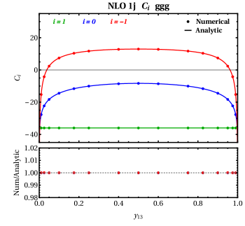
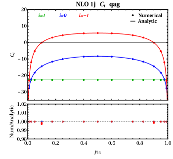
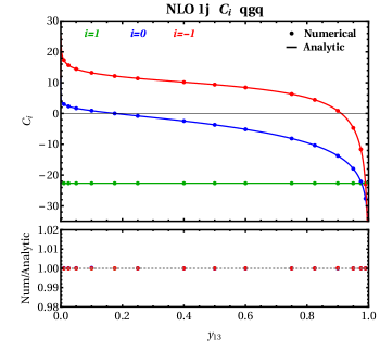
For each channel we compare the coefficients of , , and with the known analytic results in the literature Jouttenus:2011wh . We find excellent agreement with the known results for all channels and all coefficients, as demonstrated in Fig. 1. The agreement is at the level of or better.
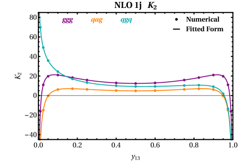
In Fig. 2 we plot the coefficient of the series expansion in of the soft function before the term has been written out using Eq. (71). The term does not contribute at NLO once is expanded, but instead enters the coefficient of in the renormalization contribution to the NNLO soft function, as shown in Eq. (3.1) and explained in detail in the next section. Since this contribution is not available in the literature, we perform a fit of our numerical results and present the fit here for completeness:
| (73) |
The coefficients are collected in Table 1. For the channels and we set (with ) since these channels are symmetrical in the initial state.
5 Soft function at NNLO
From Eq. (3.1) the renormalized -jettiness soft function at NNLO, , is
| (74) |
We have already discussed the calculation of the first term in Eq. (74) in the previous section, so we now study the second term in more detail. At NNLO three types of corrections arise: two-loop virtual corrections, one-loop corrections with one real gluon emission (“real-virtual”), and double-real corrections, consisting of the emission of and pairs. In the latter case, the emission of two gluons is made up of two diagrammatic contributions: an Abelian contribution, i.e. two single-gluon currents, and a non-Abelian contribution, i.e. emission of a pair through a three-gluon vertex. In light of this, and since the virtual two-loop corrections vanish in dimensional regularization, we can rewrite the term as the sum of four non-vanishing contributions:
| (75) |
with indicating the non-Abelian part of the double-real corrections. The Abelian term can be obtained directly from the NLO soft function thanks to well-known exponentiation theorems Frenkel:1984pz ; Gatheral:1983cz . The calculation of the real-virtual contribution is conceptually identical to the calculation of the NLO soft function and has been described in Section 3.4. We therefore spend the remainder of this section discussing the calculation of the double-real corrections represented by and . The decomposition of the relevant eikonal matrix elements into a set of basis integrals is given in Sections 3.5 and 3.6 for the and cases respectively. We will detail the transformations necessary to render the basis integrals, obtained by combining the double-emission phase space with the eikonal integrands, amenable to numerical evaluation. We will provide a number of illustrative examples of integrals, leaving a complete enumeration of all contributions to Appendix C.
5.1 Double-real corrections
We first identify a common overall factor that is associated with the total angular volume, in the phase-space parametrization of Eq. (26),
| (76) |
where
| (77) |
and is given in Eq. (34). We will always be able to trivially rescale one of the angular integrals so that the range of integration is between zero and one,
| (78) |
with , and the integral over can be recast in similar fashion,
| (79) |
by performing the change of variable . We thus rewrite Eq. (26) as,
| (80) | |||||
where we have written the remaining integral in a form that anticipates the Jacobian factor that will eventually emerge as in Eq. (78). Finally, in our eventual evaluation of the integral we will replace this form with a simpler one in which singularities can only appear at ,222An alternative procedure Anastasiou:2005qj is to split the integration range in half, into and , and then remap the second range so that all singularities are at . This method has been adopted in one of our codes.
| (81) | |||||
As before, we compute the integrals numerically using sector decomposition and the plus-distribution expansion given in Eq. (69).
As in the NLO case, the choice of the phase-space parametrization will depend upon which case is picked out by the measurement function. We will discuss each of the cases described in Section 2.3 in turn. The combination of the matrix elements, phase space, and measurement function for each case will expressed as,
| (82) |
where the coupling-associated factor is defined in Eq. (152). In this equation labels the division of the eikonal approximations, Eqs. (51), (52), and (58), and , the different cases. We have extracted an overall factor that will be universal across all contributions,
| (83) |
5.1.1 Case 1:
The appropriate change of variables for this case is,
| (84) |
We then have,
so that the combination of the phase space in Eq. (80) with the measurement function yields,
| (86) | |||||
where . In the simplest case we will be able to perform a rescaling of as in Eq. (78). However, in general this is not true.
The reason for the additional complication is the presence of the factor in the eikonal factors and . Although the Sudakov decomposition is very convenient for describing the other dot products, the expression for this one is considerably more complicated,
| (87) |
where and is the angle between and . A method for handling this denominator has been outlined in Refs. Boughezal:2015eha ; Boughezal:2013uia and we follow this strategy here. We map to a new variable through the relation,
| (88) |
or the inverse,
| (89) |
The Jacobian associated with the transformation from to is,
| (90) |
In terms of the new variable we have,
| (91) |
so that
| (92) |
Further, from Eq. (88) we have that,
| (93) |
We observe that by means of this change of variable the collinear singularity has been mapped to . In the presence of this denominator (and associated factor of ) we must be careful to ensure that the relevant angles are handled appropriately. It is convenient to perform the integration in a rotated frame, c.f. Appendix B. Following that logic, we replace the measure with and, from Eq. (150), relate the angle to , , and through,
| (94) |
The final integral in Eq. (86) then becomes,
| (95) | |||||
where . Thus the final form for the phase space is,
| (96) | |||||
where , , is defined through Eq. (93), and can be obtained from Eq. (94).
The matrix elements that must be evaluated to compute the double-real contributions for this case are given in Appendix C.1. They are expressed in terms of the new variables , , and and to aid in the evaluation of contribution they have been further subdivided into integrals that are simpler to compute.
To illustrate a further complication that arises for these integrals, consider the evaluation of contribution . Combining the phase space from Eq. (96) with the matrix element in Eq. (153) we obtain,
| (97) | |||||
where is given in Eq. (77) and we have removed an overall factor of in the definition of , c.f. Eq. (82). In order to be able to perform the integration, we have to handle the line singularity associated with the term. Following Ref. Boughezal:2015eha , we do so by partitioning the integral into two contributions by means of the identity,
| (98) |
In the sector we then perform the change of variables
| (99) |
while in the sector we have
| (100) |
such that, in general, all singularities are located at and . The only complication is that, for the integrand , this procedure also yields singularities at . However, these are simple to handle by using a simplification similar to the one in Eq. (81), but carried out for . These transformations are sufficient to treat all of the singularities in this case.
5.1.2 Case 2:
The change of variables for this case is,
| (101) |
In combination with the measurement function, this results in a phase-space parametrization that is very similar to the simplest one for case 1,
| (102) | |||||
where and . The remaining invariant that enters the matrix elements (given in Appendix C.2) becomes,
| (103) |
where and is obtained from, c.f. Eq. (146),
| (104) |
This does not require any further reparametrization of the phase space because factors of do not lead to singularities as .
5.1.3 Case 3:
This case uses the following change of variables, based on a Sudakov expansion with respect to and ,
| (105) |
The phase-space parametrization becomes,
| (106) | |||||
where and . Since one of the emitting lines is no longer one of the vectors in the Sudakov expansion, more invariants must be defined. The remaining quantities are,
| (107) |
where and is again defined through Eq. (146). There are no further singularities to disentangle in this case, for which all matrix elements are specified in Appendix C.3.
5.1.4 Case 4:
We perform the Sudakov expansion with respect to base vectors and and then the following change of variables,
| (108) |
After this transformation the phase space parametrization is,
| (109) | |||||
The other invariants that enter the matrix elements are,
| (110) |
Since this denominator takes the same form as the one considered in case 1, it must be handled in a similar manner. Explicitly we have,
| (111) | |||||
where the definitions of all the angles are taken over from case 1.
The matrix elements for this case are given in Appendix C.3. In the calculation of the contribution an additional subtlety arises. Consider the evaluation of the sector that appears after the partitioning of Eq. (98). Following the change of variables in Eq. (99) we have,
| (112) | |||||
The penultimate line of this equation appears to indicate that a plus-distribution expansion is required for and that the integration is too singular as (i.e. in the original variables). However, a careful analysis reveals that neither of these is true. Instead, these additional denominator factors are actually regulated by the numerator, . To see that this is the case we write out the expressions for explicitly and use the the relation between the angles in Eq. (94) to find,
| (113) | |||
This expression makes it clear that the denominator factor is harmless. Moreover, we observe that in the limit ,
| (114) |
so that,
| (115) | |||||
The use of this limit is essential in order to obtain the correct subtraction of the singularity at .
6 Results
We first make a few observations regarding our numerical integration procedure. Each contributing integral is computed using VEGAS in double precision. Since many of the integrals contain square-root singularities, we routinely perform remappings to remove such factors and improve the convergence of the numerical integration,
| (116) |
Moreover, in order to avoid numerical instability when evaluating the double-real integrands extremely close to singularities, we impose a tiny cut on every integration range:
| (117) |
We do not observe any sensitivity of our results to reasonable variations of , within Monte Carlo uncertainties, and choose for the final results presented below. We have additionally checked that running the code in quadruple precision with a cutoff reduced to does not alter the results. In order to provide the reader with an example of our raw results, and a point of comparison for an independent implementation, we present the numerical value of all double-real integrals at a single phase-space point in Appendix D. Each integral is typically evaluated with an uncertainty that is far smaller than one percent, but which can be at the percent level for a few contributions where the absolute value is very small. This accuracy is more than sufficient to obtain the NNLO soft function at the level necessary for phenomenology.
Having described all of the necessary ingredients to perform the calculations, we can now present our numerical results for the - and -jettiness soft functions at NNLO. In particular, we focus on the non-Abelian contribution to the soft functions. Following the notation of Sec. 5, we define the non-Abelian part of the NNLO soft function as the sum of four different contributions:
| (118) |
Each individual contribution is computed as explained in the previous sections. After performing the sum, the non-Abelian soft function corresponds to the contribution to the total. This is written as
| (119) |
where with are numerical coefficients, functions of the invariants .
6.1 -jettiness
Although the calculation of the -jettiness soft function is the focus of this paper, recomputing the -jettiness soft function provides a useful check of a subset of the integrals and of the assembly of the final result. In this case the result is known analytically Kelley:2011ng ; Monni:2011gb , which we can use to provide a robust check of our calculation.
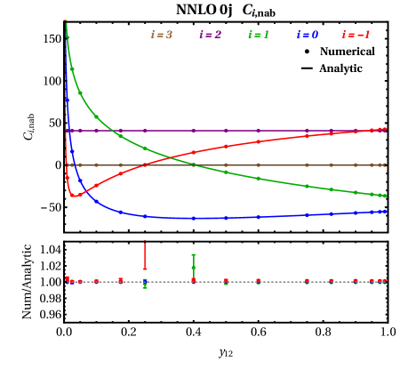
We choose to present our results using the color factor (i.e. the partons present at leading order are a quark and an anti-quark) and compute the coefficients for 15 different values of (the only invariant in the case of -jettiness):
| (120) |
The channel is obtained by simply rescaling by a factor . A comparison of our numerical evaluation of the NNLO soft function with the analytic results, for the values of above, is shown in Fig. 3. Apart from regions where the soft functions are very close to zero, the numerical and analytic results agree perfectly, at the level of a few per-mille or better.
6.2 -jettiness
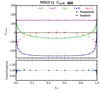
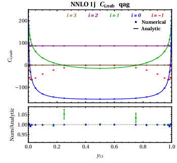
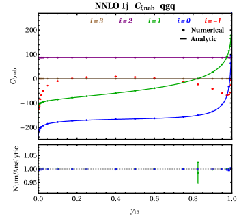
We present the non-Abelian contribution to the -jettiness soft function. As in the NLO case, we specialize our calculation for LHC kinematics. The coefficients are functions of only since and . We compute the coefficients for the three different partonic configurations (, , and ) and for 21 different values of :
| (121) |
The coefficients – are known analytically and can be derived, for instance, from renormalization group constraints Jouttenus:2011wh ; Boughezal:2015eha ; Gaunt:2015pea . They therefore provide a useful check of our calculation, particularly in the case of , which receives contributions from all the basis integrals and expansions that must be performed for . Our results are shown in Fig. 4 and indicate that, as at NLO, the numerical integration is accurate to the per-mille level when compared with the analytic results for –.
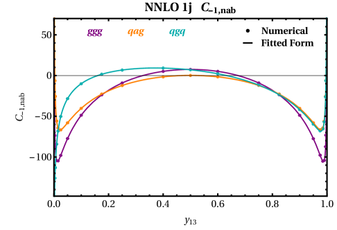
The calculation of the endpoint contribution is the central result of this paper. Our results for this contribution are shown separately in Fig. 5, for each of the three configurations. We have performed fits to our results using the functional form,
| (122) |
and these fits are also shown in the figure. Uncertainties on the fits are estimated at the 95% confidence level, and are plotted in the figure (they essentially correspond to the line thickness). The fits provide a very good description of the endpoint coefficient and are far more efficient for subsequent evaluation of the soft function. The values of the fit coefficients of Eq. (122) for the three cases are collected in Table 2. For the channels and we set (with ). We have tested the fits using randomly-generated phase-space points for comparison and within their respective MC uncertainties every event agrees with the prediction from the fits. When the MC uncertainties are small the agreement is within , while for points for which the coefficients are close to zero the MC uncertainties are significantly larger and the agreement is at the few percent level.
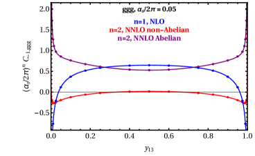
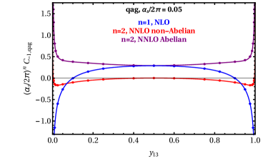
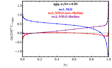
To assess the overall impact of the corrections to the soft function, in Fig. 6 we show the NLO contribution along with the Abelian and non-Abelian pieces of the NNLO contribution. It is clear that the Abelian pieces are significantly larger than the non-Abelian pieces over the entire phase space for each partonic configuration. This can be readily understood from the analytic structures of the two pieces. The coefficient of the Abelian part arises from the convolution of the NLO result with itself, and therefore it has two contributing parts. Firstly, there is the “pure” piece, which arises from the coefficient of the NLO soft function squared. This term is comparable to the non-Abelian part in size. Secondly, there are mixed contributions which arise from convolutions of the form
| (123) |
where the coefficients can be found, for instance, in Table 1 of Ref. Gaunt:2015pea , and are roughly . After both contributions are combined together the dominant part of the total coefficient is determined by the term. Such a term is not present in the non-Abelian calculation.
6.3 Generic kinematics
Finally, we compute the non-Abelian part of the 1-jettiness soft function at NNLO with generic kinematics, i.e. for the case where the scattering process has three colored partons at Born level, but where two of them do not represent the directions of incoming beams (as is the case for LHC kinematics). We parametrize the three directions , , and as
| (124) |
with and . For the invariants (with ) we therefore explicitly have
| (125) |
We observe that with this parametrization the LHC limit is recovered by setting and . We compute the coefficients of the non-Abelian part of the soft function for the three different partonic configurations (, , and ) by choosing 200 random values for , , and . We then perform numerical fits to our results for the coefficient of , . The functional form of the fits is taken to be
| (126) |
In order to obtain accurate fits, we retain all 64 coefficients in Eq. (126) for each partonic channel. The values of the coefficients for the three cases are collected in ancillary files that we include in the arXiv submission.
We can test the validity of the generic fits by ensuring that they correctly reproduce the dedicated LHC fits obtained in Section 6.2 when choosing and in Eq. (126). We therefore define the following ratio
| (127) |
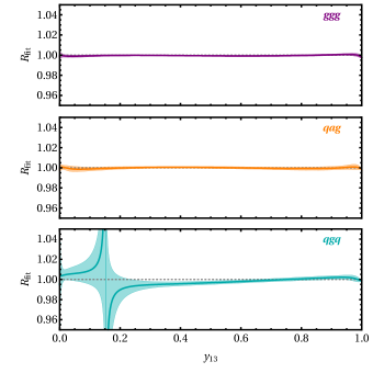
In the above equation represents the coefficient of the Abelian part of the soft function (evaluated for LHC kinematics). We have added it to the numerator and denominator such that compares the total NNLO coefficients using the two different fits. This combination is the only one that is relevant for phenomenological applications. In addition, since vanishes for certain values of , the sum of Abelian and non-Abelian pieces helps to ensure that the ratio is not dominated by the regions in which one of the fits is close to zero. The ratios of the two fits are shown in the left panel of Fig. 7. By inspecting Fig. 7 we see that for the and channels the generic fit reproduces the dedicated LHC fit to better than 1%. On the other hand, the channel is poorly behaved in the region . This is due to the vanishing of both the Abelian and the non-Abelian pieces in this region, which causes large sensitivity to fitting uncertainties. Away from this region the general fit does a good job (within 1%) at reproducing the dedicated LHC fit.
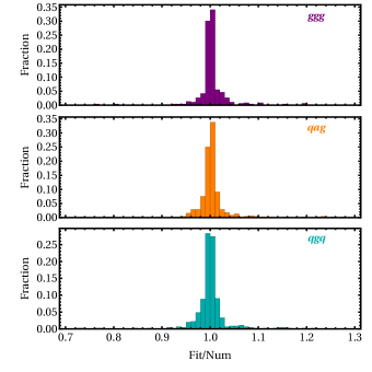
Additionally, as in the LHC case, we can test the fits by generating random phase-space points and comparing the numerical results of the non-Abelian piece with the predicted values from the corresponding fits. In this case we perform the comparison by generating 450 phase-space points and plotting the ratios between fit and numerical values as histograms. The results are shown in the right panel of Fig. 7. We observe that for all three channels the histograms are well-centered around the value of . In particular, the values obtained with the fit lie within of a dedicated calculation of a configuration for , , and of the total number of random phase-space points respectively (, , and ), and within for , , and of the phase-space points. Similarly to the LHC case, the agreement between fitted and numerical values is better for points with smaller MC uncertainties and coefficients that are not close to zero. We therefore believe that the fits of Eq. (126), which are valid for non-LHC kinematics, could be successfully used, for instance, in and applications.
7 Conclusions
In this paper we have presented a calculation of the next-to-next-to leading order (NNLO) 1-jettiness soft function. The soft function is a component part of NNLO calculations which employ slicing methods based on the -jettiness global event shape variable. In particular, this function is a required piece of the calculation of differential type processes at NNLO, in which represents a color singlet, for instance a single vector boson.
Our calculation bears the traditional hallmarks of NNLO calculations in regards to its complexity in unresolved limits. In order to deal with these issues we have employed a numerical approach which uses sector decomposition of the relevant phase-space integrals to disentangle overlapping singularities present at this order. In order to ensure the correctness of our results we have implemented two completely independent computational codes, and validated them against one another. We have further validated our results by recomputing the known 0-jettiness and 1-jettiness results at NNLO and NLO accuracy respectively. As a final validation of our results we have checked the known analytic pieces of the 1-jettiness soft function at NNLO that can be derived from renormalization group arguments. The primary result of our calculation is a numerical determination of the endpoint contribution, which cannot be deduced from the RGE’s alone. We have computed this contribution for LHC kinematics (scattering processes with two back-to-back partons and one final-state jet at Born level) and for generic kinematics (three colored partons at leading order). In order to disseminate our results we have produced polynomial fits to the results of our numerical integration for both configurations. We have additionally checked both fits using randomly-generated phase-space points, and find excellent agreement with our Monte Carlo output.
Our fits represent the first such results presented in the literature. A previous calculation of the -jettiness soft function at NNLO for LHC kinematics has been published Boughezal:2015eha . It does not contain the information required to implement the results in a standalone Monte Carlo program. We therefore believe our calculation, and the corresponding numerical fits, will be useful for those interested in applying jettiness-slicing and subtraction methods to NNLO calculations where three colored particles are present. Further applications of this method are certainly possible in future, for instance to analyze a variety of global event shape definitions or to increase the number of partonic scatters under consideration, such as in the calculation of the 2-jettiness soft function at NNLO. We leave such applications to a future study.
Acknowledgments
R.K.E would like to acknowledge the hospitality of the Fermilab theory group, where this work was initiated, and SUNY (Buffalo) where it was completed. C.W. and R.M. are supported by a National Science Foundation CAREER award PHY-1652066. Support provided by the Center for Computational Research at the University at Buffalo. This manuscript has been authored by Fermi Research Alliance, LLC under Contract No. DE-AC02-07CH11359 with the U.S. Department of Energy, Office of Science, Office of High Energy Physics. The U.S. Government retains and the publisher, by accepting the article for publication, acknowledges that the U.S. Government retains a non-exclusive, paid-up, irrevocable, world-wide license to publish or reproduce the published form of this manuscript, or allow others to do so, for U.S. Government purposes.
Appendix A Dimensional regularization
A -dimensional Euclidean integral may be written as,
| (128) | |||||
The range of the angular integrals is except for . Eq. (128) is best proved by induction. Assuming that it is true for a -dimensional integral, in dimensions we can write,
The -dimensional length, , can be written in terms of the -dimensional length, , as
| (131) |
Changing variables to and we recover the -dimensional version of Eq. (128).
For our particular case at hand we have :
| (132) | |||||
| (133) | |||||
A -dimensional vector can be written as,
| (134) |
where the components before the semi-colon are the extra-dimensional pieces and the vector is a unit vector in the first extra dimension. We arrive at this frame by setting for . Let us choose vectors in the transverse plane given by
| (135) |
so that for we have set , and for we set , . The integral over unconstrained angles is,
| (136) |
so that, after integrating over them, we get the following expression
| (137) | |||||
where
| (138) |
By performing the integration over we get
| (139) | |||||
Using the standard result,
| (140) |
the total volume of angular integration is
| (141) |
Appendix B Rotational invariance of the solid angle integral measure
Perform an angle-radius decomposition of the coordinates
| (142) |
where is a coordinate in the transverse plane beyond the usual two. Hence
| (143) |
Now perform a rotation about the -axis by an angle :
| (144) |
These coordinates can also be parametrized by introducing new angles,
| (145) | |||||
Comparing the two parametrizations, we note that
| (146) | |||||
| (147) |
Calculating the solid element, we see that
| (148) | |||||
| (149) |
as can be shown by explicitly calculating the Jacobian for the transformation. However, after the change of variables , we must be sure to express all dependence on in terms of and ,
| (150) |
Appendix C Double-real matrix elements
Here we list the expressions for the matrix elements , defined in Eqs. (51), (52), and (58), that must be integrated to evaluate the double-real contributions. The expressions depend on the case specified by the measurement function, which determines the choice of the Sudakov directions. For it is useful to perform a further decomposition to aid the numerical integration of these contributions, with the division of terms depending on the case at hand. We have,
| (151) |
for cases 1 and 4, while the sum only runs over the and terms for cases 2 and 3.
We note that in the eventual evaluation of these matrix elements we must restore an overall factor,
| (152) |
C.1 Case 1
Using the relations in Eq. (84) and the transformation of Eq. (91) we have,
| (153) | |||||
| (154) | |||||
| (155) | |||||
| (156) | |||||
| (158) |
We note that since does not depend on it may be treated using the phase-space measure in Eq. (86). All other contributions require the use of Eq. (96) and the further partitioning indicated in Eq. (98).
C.2 Case 2
C.3 Case 3
C.4 Case 4
Appendix D Results for double-real integrals
Results for the coefficient of each of the basic integrals entering the double-real emission calculation, at a sample phase-space point, are given in Table 3. These coefficients are the ones that enter the calculation of the endpoint contribution to the NNLO soft function and may be useful to the reader interested in reproducing the results of our calculation.
| Case | Integral | Result |
|---|---|---|
| C1I | ||
| C1II | ||
| C1IIIa | ||
| C1IIIb | ||
| C1IIIc | ||
| C1IIId | ||
| C1III | ||
| C1I | ||
| C1II | ||
| C1IIIa | ||
| C1IIIb | ||
| C1IIIc | ||
| C1IIId | ||
| C1III | ||
| C2I | ||
| C2II | ||
| C2IIIa | ||
| C2IIIb | ||
| C2III | ||
| C3I | ||
| C3II | ||
| C3IIIa | ||
| C3IIIb | ||
| C3III | ||
| C3I | ||
| C3II | ||
| C3IIIa | ||
| C3IIIb | ||
| C3III | ||
| C4I | ||
| C4II | ||
| C4IIIa | ||
| C4IIIb | ||
| C4IIIc | ||
| C4IIId | ||
| C4III |
Appendix E Analytic result for -jettiness at NLO
For LHC kinematics, the -jettiness case refers to processes with two initial-state colored partons and no final-state jets (plus any non-colored final-state particle). The only allowed leading-order configurations are therefore either a pair of gluons or a quark-antiquark pair. For the purposes of our calculation, this means that and that we need not consider the phase-space sector . Moreover, there is no -function involving an angle left in the problem. As discussed in Section 3.3, color conservation means that the overall color factor, , is given by either for a quark-antiquark pair or for a pair of gluons. The -jettiness soft function at NLO is thus given by Eq. (3.2) after setting . The phase-space integrals can then be performed analytically so that the soft function reads,
| (173) | ||||
where . The result in Eq. (173) agrees with Eq. (52) of Ref. Jouttenus:2011wh after taking into account the different notation and overall normalization. By performing the expansion of Eq. (71) on the result in Eq. (173), and keeping the physical term, we find:
| (174) |
For color-singlet production at the LHC the two initial-state partons are back-to-back so that () and the soft function simplifies to,
| (175) |
This result agrees with the literature (c.f. Eq. (173) of Ref. Fleming:2007xt and Eq. (2.23) of
Ref. Berger:2010xi ). The more general result of Eq. (174) can be used for or processes with
respectively one or two final-state jets.
References
- (1) J. Currie, A. Gehrmann-De Ridder, T. Gehrmann, N. Glover, J. Pires and S. Wells, Second order QCD corrections to gluonic jet production at hadron colliders, PoS LL2014 (2014) 001 [1407.5558].
- (2) J. Currie, E. W. N. Glover and J. Pires, NNLO QCD predictions for single jet inclusive production at the LHC, 1611.01460.
- (3) A. Gehrmann-De Ridder, T. Gehrmann, N. Glover, A. Huss and T. A. Morgan, NNLO QCD corrections for boson plus jet production, PoS RADCOR2015 (2016) 075 [1601.04569].
- (4) A. Gehrmann-De Ridder, T. Gehrmann, E. W. N. Glover, A. Huss and T. A. Morgan, Precise QCD predictions for the production of a Z boson in association with a hadronic jet, Phys. Rev. Lett. 117 (2016), no. 2 022001 [1507.02850].
- (5) A. Gehrmann-De Ridder, T. Gehrmann, E. W. N. Glover, A. Huss and T. A. Morgan, The NNLO QCD corrections to Z boson production at large transverse momentum, JHEP 07 (2016) 133 [1605.04295].
- (6) R. Boughezal, J. M. Campbell, R. K. Ellis, C. Focke, W. T. Giele, X. Liu and F. Petriello, Z-boson production in association with a jet at next-to-next-to-leading order in perturbative QCD, Phys. Rev. Lett. 116 (2016), no. 15 152001 [1512.01291].
- (7) R. Boughezal, X. Liu and F. Petriello, W-boson plus jet differential distributions at NNLO in QCD, Phys. Rev. D94 (2016), no. 11 113009 [1602.06965].
- (8) J. M. Campbell, R. K. Ellis and C. Williams, Direct Photon Production at Next-to-Next-to-Leading Order, Phys. Rev. Lett. 118 (2017), no. 22 222001 [1612.04333].
- (9) J. M. Campbell, R. K. Ellis and C. Williams, Driving missing data at the LHC: NNLO predictions for the ratio of and , Phys. Rev. D96 (2017), no. 1 014037 [1703.10109].
- (10) R. Boughezal, F. Caola, K. Melnikov, F. Petriello and M. Schulze, Higgs boson production in association with a jet at next-to-next-to-leading order, Phys. Rev. Lett. 115 (2015), no. 8 082003 [1504.07922].
- (11) R. Boughezal, C. Focke, W. Giele, X. Liu and F. Petriello, Higgs boson production in association with a jet at NNLO using jettiness subtraction, Phys. Lett. B748 (2015) 5–8 [1505.03893].
- (12) X. Chen, J. Cruz-Martinez, T. Gehrmann, E. W. N. Glover and M. Jaquier, NNLO QCD corrections to Higgs boson production at large transverse momentum, JHEP 10 (2016) 066 [1607.08817].
- (13) M. Cacciari, F. A. Dreyer, A. Karlberg, G. P. Salam and G. Zanderighi, Fully Differential Vector-Boson-Fusion Higgs Production at Next-to-Next-to-Leading Order, Phys. Rev. Lett. 115 (2015), no. 8 082002 [1506.02660].
- (14) M. Brucherseifer, F. Caola and K. Melnikov, On the NNLO QCD corrections to single-top production at the LHC, Phys. Lett. B736 (2014) 58–63 [1404.7116].
- (15) E. L. Berger, J. Gao, C. P. Yuan and H. X. Zhu, NNLO QCD Corrections to t-channel Single Top-Quark Production and Decay, Phys. Rev. D94 (2016), no. 7 071501 [1606.08463].
- (16) E. L. Berger, J. Gao and H. X. Zhu, Differential Distributions for t-channel Single Top-Quark Production and Decay at Next-to-Next-to-Leading Order in QCD, 1708.09405.
- (17) M. Czakon, P. Fiedler, D. Heymes and A. Mitov, NNLO QCD predictions for fully-differential top-quark pair production at the Tevatron, JHEP 05 (2016) 034 [1601.05375].
- (18) R. K. Ellis, D. A. Ross and A. E. Terrano, The Perturbative Calculation of Jet Structure in Annihilation, Nucl. Phys. B178 (1981) 421–456.
- (19) Z. Kunszt, P. Nason, G. Marchesini and B. R. Webber, QCD AT LEP, in LEP Physics Workshop Geneva, Switzerland, February 20, 1989, pp. 373–453, 1989.
- (20) S. Catani and M. H. Seymour, A General algorithm for calculating jet cross-sections in NLO QCD, Nucl. Phys. B485 (1997) 291–419 [hep-ph/9605323]. [Erratum: Nucl. Phys.B510,503(1998)].
- (21) A. Gehrmann-De Ridder, T. Gehrmann and E. W. N. Glover, Antenna subtraction at NNLO, JHEP 09 (2005) 056 [hep-ph/0505111].
- (22) G. Somogyi, Z. Trócsányi and V. Del Duca, A Subtraction scheme for computing QCD jet cross sections at NNLO: Regularization of doubly-real emissions, JHEP 0701 (2007) 070 [hep-ph/0609042].
- (23) M. Czakon, A novel subtraction scheme for double-real radiation at NNLO, Phys. Lett. B693 (2010) 259–268 [1005.0274].
- (24) A. Gehrmann-De Ridder, T. Gehrmann and M. Ritzmann, Antenna subtraction at NNLO with hadronic initial states: double real initial-initial configurations, JHEP 10 (2012) 047 [1207.5779].
- (25) F. Caola, K. Melnikov and R. R ntsch, Nested soft-collinear subtractions in NNLO QCD computations, Eur. Phys. J. C77 (2017), no. 4 248 [1702.01352].
- (26) W. T. Giele, E. W. N. Glover and D. A. Kosower, Higher order corrections to jet cross-sections in hadron colliders, Nucl. Phys. B403 (1993) 633–670 [hep-ph/9302225].
- (27) S. Catani and M. Grazzini, An NNLO subtraction formalism in hadron collisions and its application to Higgs boson production at the LHC, Phys. Rev. Lett. 98 (2007) 222002 [hep-ph/0703012].
- (28) J. C. Collins, D. E. Soper and G. F. Sterman, Transverse Momentum Distribution in Drell-Yan Pair and W and Z Boson Production, Nucl. Phys. B250 (1985) 199–224.
- (29) R. Boughezal, C. Focke, X. Liu and F. Petriello, -boson production in association with a jet at next-to-next-to-leading order in perturbative QCD, Phys. Rev. Lett. 115 (2015), no. 6 062002 [1504.02131].
- (30) J. Gaunt, M. Stahlhofen, F. J. Tackmann and J. R. Walsh, N-jettiness Subtractions for NNLO QCD Calculations, JHEP 09 (2015) 058 [1505.04794].
- (31) I. W. Stewart, F. J. Tackmann and W. J. Waalewijn, N-Jettiness: An Inclusive Event Shape to Veto Jets, Phys. Rev. Lett. 105 (2010) 092002 [1004.2489].
- (32) C. W. Bauer, S. Fleming and M. E. Luke, Summing Sudakov logarithms in in effective field theory, Phys. Rev. D63 (2000) 014006 [hep-ph/0005275].
- (33) C. W. Bauer, S. Fleming, D. Pirjol and I. W. Stewart, An Effective field theory for collinear and soft gluons: Heavy to light decays, Phys. Rev. D63 (2001) 114020 [hep-ph/0011336].
- (34) C. W. Bauer and I. W. Stewart, Invariant operators in collinear effective theory, Phys. Lett. B516 (2001) 134–142 [hep-ph/0107001].
- (35) C. W. Bauer, D. Pirjol and I. W. Stewart, Soft collinear factorization in effective field theory, Phys. Rev. D65 (2002) 054022 [hep-ph/0109045].
- (36) C. W. Bauer, S. Fleming, D. Pirjol, I. Z. Rothstein and I. W. Stewart, Hard scattering factorization from effective field theory, Phys. Rev. D66 (2002) 014017 [hep-ph/0202088].
- (37) J. Gaunt, M. Stahlhofen and F. J. Tackmann, The Gluon Beam Function at Two Loops, JHEP 08 (2014) 020 [1405.1044].
- (38) J. R. Gaunt, M. Stahlhofen and F. J. Tackmann, The Quark Beam Function at Two Loops, JHEP 04 (2014) 113 [1401.5478].
- (39) T. T. Jouttenus, I. W. Stewart, F. J. Tackmann and W. J. Waalewijn, The Soft Function for Exclusive N-Jet Production at Hadron Colliders, Phys. Rev. D83 (2011) 114030 [1102.4344].
- (40) R. Boughezal, X. Liu and F. Petriello, -jettiness soft function at next-to-next-to-leading order, Phys. Rev. D91 (2015), no. 9 094035 [1504.02540].
- (41) S. Catani and M. Grazzini, The soft gluon current at one loop order, Nucl. Phys. B591 (2000) 435–454 [hep-ph/0007142].
- (42) J. M. Campbell and E. W. N. Glover, Double unresolved approximations to multiparton scattering amplitudes, Nucl. Phys. B527 (1998) 264–288 [hep-ph/9710255].
- (43) S. Catani and M. Grazzini, Infrared factorization of tree level QCD amplitudes at the next-to-next-to-leading order and beyond, Nucl. Phys. B570 (2000) 287–325 [hep-ph/9908523].
- (44) C. Anastasiou, K. Melnikov and F. Petriello, A new method for real radiation at NNLO, Phys. Rev. D69 (2004) 076010 [hep-ph/0311311].
- (45) R. Boughezal, K. Melnikov and F. Petriello, A subtraction scheme for NNLO computations, Phys. Rev. D85 (2012) 034025 [1111.7041].
- (46) J. Frenkel and J. C. Taylor, Nonabelian Eikonal Exponentiation, Nucl. Phys. B246 (1984) 231–245.
- (47) J. G. M. Gatheral, Exponentiation of Eikonal Cross-sections in Nonabelian Gauge Theories, Phys. Lett. 133B (1983) 90–94.
- (48) C. Anastasiou, K. Melnikov and F. Petriello, Fully differential Higgs boson production and the di-photon signal through next-to-next-to-leading order, Nucl. Phys. B724 (2005) 197–246 [hep-ph/0501130].
- (49) R. Boughezal, F. Caola, K. Melnikov, F. Petriello and M. Schulze, Higgs boson production in association with a jet at next-to-next-to-leading order in perturbative QCD, JHEP 06 (2013) 072 [1302.6216].
- (50) R. Kelley, M. D. Schwartz, R. M. Schabinger and H. X. Zhu, The two-loop hemisphere soft function, Phys. Rev. D84 (2011) 045022 [1105.3676].
- (51) P. F. Monni, T. Gehrmann and G. Luisoni, Two-Loop Soft Corrections and Resummation of the Thrust Distribution in the Dijet Region, JHEP 08 (2011) 010 [1105.4560].
- (52) S. Fleming, A. H. Hoang, S. Mantry and I. W. Stewart, Top Jets in the Peak Region: Factorization Analysis with NLL Resummation, Phys. Rev. D77 (2008) 114003 [0711.2079].
- (53) C. F. Berger, C. Marcantonini, I. W. Stewart, F. J. Tackmann and W. J. Waalewijn, Higgs Production with a Central Jet Veto at NNLL+NNLO, JHEP 04 (2011) 092 [1012.4480].