Denoising Gravitational Waves using Deep Learning
with Recurrent Denoising Autoencoders

Abstract

Gravitational wave astronomy is a rapidly growing field of modern astrophysics, with observations being made frequently by the LIGO detectors. Gravitational wave signals are often extremely weak and the data from the detectors, such as LIGO, is contaminated with non-Gaussian and non-stationary noise, often containing transient disturbances which can obscure real signals. Traditional denoising methods, such as principal component analysis and dictionary learning, are not optimal for dealing with this non-Gaussian noise, especially for low signal-to-noise ratio gravitational wave signals. Furthermore, these methods are computationally expensive on large datasets. To overcome these issues, we apply state-of-the-art signal processing techniques, based on recent groundbreaking advancements in deep learning, to denoise gravitational wave signals embedded either in Gaussian noise or in real LIGO noise. We introduce SMTDAE, a Staired Multi-Timestep Denoising Autoencoder, based on sequence-to-sequence bi-directional Long-Short-Term-Memory recurrent neural networks. We demonstrate the advantages of using our unsupervised deep learning approach and show that, after training only using simulated Gaussian noise, SMTDAE achieves superior recovery performance for gravitational wave signals embedded in real non-Gaussian LIGO noise.

I Introduction

The application of machine learning and deep learning techniques have recently driven disruptive advances across many domains in engineering, science, and technology LeCun et al. (2015). The use of these novel methodologies is gaining interest in the gravitational wave (GW) community. Convolutional neural networks were recently applied for the detection and characterization of GW signals in real-time George and Huerta (2016, 2017a). The use of machine learning algorithms have also been explored to address long-term challenges in GW data analysis for classification of the imprints of instrumental and environmental noise from GW signals Powell et al. (2015, 2016); Zevin et al. (2016); George et al. (2017a, b), and also for waveform modeling Huerta et al. (2017). Torres et al. (2015, 2014, 2016a) introduced a variety of methods to recover GW signals embedded in additive Gaussian noise.

PCA is widely used for dimension reduction and denoising of large datasets Jolliffe (2002); Anderson (2003). This technique was originally designed for Gaussian data and its extension to non-Gaussian noise is a topic of ongoing research Jolliffe (2002). Dictionary learning Mairal et al. (2009a); Hawe et al. (2013); Mairal et al. (2009b) is an unsupervised technique to learn an overcomplete dictionary that contains single-atoms from the data, such that the signals can be described by sparse linear combinations of these atoms Aharon et al. (2006); Baraniuk et al. (2010). Exploiting the sparsity is useful for denoising, as discussed in Baraniuk et al. (2010); Gribonval and Nielsen (2006); Mairal et al. (2009a); Hawe et al. (2013); Mairal et al. (2009b). Given the dictionary atoms, the coefficients are estimated by minimizing an error term and a sparsity term, using a fast iterative shrinkage-thresholding algorithm Beck and Teboulle (2009).

Dictionary learning was recently applied to denoise GW signals embedded in Gaussian noise whose peak signal-to-noise ratio (SNR)$\sim 1$ Torres et al. (2016b). This involves learning a group of dictionary atoms from true GW signals, and then reconstructing signals in a similar fashion to PCA, i.e., by combining different atoms with their corresponding weights. However, the drawback is that coefficients are not simply retrieved from projections but learned using $L_{1}$ minimization. Therefore, denoising a single signal requires running $L_{1}$ minimization repeatedly, which is a bottleneck that inevitably leads to delays in the analysis. Furthermore, it is still challenging to estimate both the dictionary and the sparse coefficients of the underlying clean signal when the data is contaminated with non-Gaussian noise Chainais (2012); Giryes and Elad (2014).

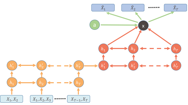
To address the aforementioned challenges, we introduce an unsupervised learning technique using a new model which we call Staired Multi-Timestep Denoising Autoencoder (SMTDAE), that is inspired by the recurrent neural networks (RNNs) used for noise reduction introduced in Maas et al. (2012). The structure of the SMTDAE model is shown in FIG 1(b). RNNs are the state-of-the-art generic models for continuous time-correlated machine learning problems, such as speech recognition/generation Graves et al. (2013); Arik et al. (2017); Zhang et al. (2017), natural language processing/translation Sutskever et al. (2014), handwriting recognition Graves and Schmidhuber (2009), etc. A Denoising Autoencoder (DAE) is an unsupervised learning model that takes noisy signals and return the clean signals Bengio et al. (2013); Vincent et al. (2008, 2010); Maas et al. (2012). By combining the advantages of the two models, we demonstrate excellent recovery of weak GW signals injected into real LIGO noise based on the two measurements, Mean Square Error (MSE) and Overlap  Dal Canton et al. (2014); Usman et al. (2016). Our results show that SMTDAE outperforms denoising methods based on PCA and dictionary learning using both metrics.

(a) MTDAE

(b) SMTDAE

(c) Reference

Figure 1: 1(a) shows the structure of MTDAE. This model passes multiple inputs of a noisy waveform into hidden layers constructed with LSTM cells and outputs a clean version. The timestep in the output is the middle timestep in each of the multiple inputs. 1(b) indicates our proposed SMTDAE structure that uses a sequence-to-sequence model. It differs from MTDAE in that the final state of encoder is passed to the beginning state of decoder in hidden layers. We also include a Signal Amplifier before the output layer in the network to enhance signal reconstruction. The nomenclature is described in 1(c).

II Methods

The noise present in GW detectors is highly non-Gaussian, with a time-varying (non-stationary) power spectral density. Our goal is to extract clean GW signals from the noisy data stream from a single LIGO detector. Since this is a time-dependent process, we need to ensure that SMTDAE can recover a signal given noisy signal input and return zeros given pure noise.

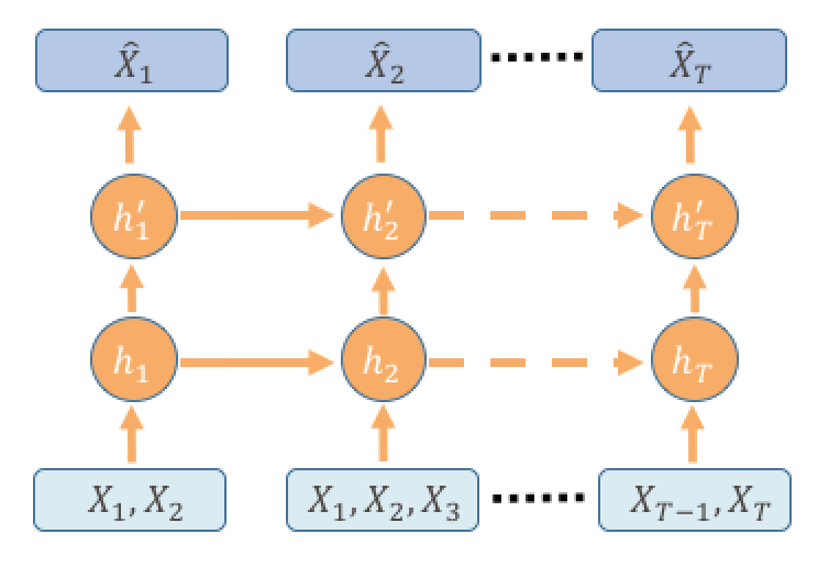
Denoising GWs is similar to removing noise in automatic speech recognition (ASR) through RNN, as illustrated in FIG 1(a). The state-of-the-art tool in ASR is the Multiple Timestep Denoising Autoencoder (MTDAE), introduced in Maas et al. (2012). The idea of this model is to take multiple time steps within a neighborhood to predict the value of a specific point. Compared to conventional RNNs, which takes only one time step input to predict the value of that corresponding output, MTDAE takes one time step and its neighbors to predict one output. It is shown in Maas et al. (2012) that this model returns better denoised outputs.

Realizing the striking similarities between ASR and denoising GWs, we have constructed a Staired Multiple Timestep Denoising Autoencoder (SMTDAE). As shown in FIG 1(b), our new model encodes the actual physics of the problem we want to address by including the following novel features:

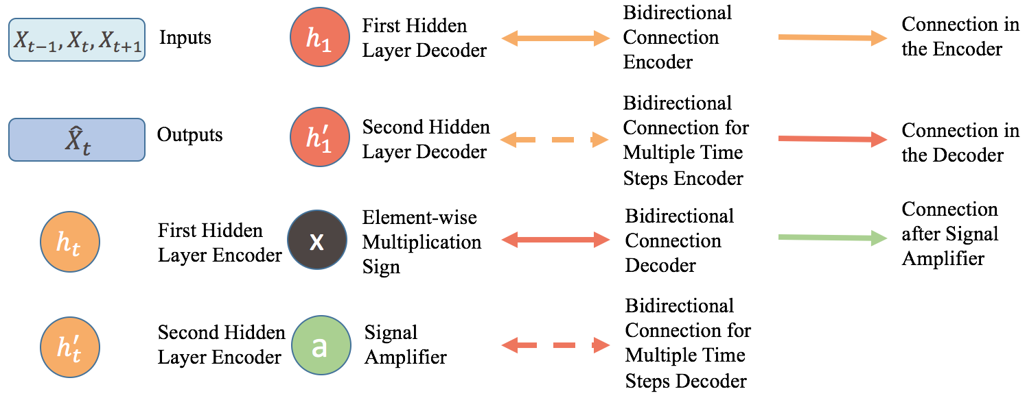
• Since GW detection is a time-dependent analysis, our encoder and decoder have time-correlations, as shown in FIG 1(b). The final state that records information of the encoder will be passed to the first state of the decoder. We use a sequence-to-sequence model Sutskever et al. (2014) with two layers for the encoder and decoder, where each layer uses a bidirectional LSTM cell Hochreiter and Schmidhuber (1997). This type of structure is widely used in Natural Language Processing (NLP) .

• We have included another scalar variable which we call Signal Amplifier—indicated by a green circle in FIG 1(b). This is extremely helpful in denoising GW signals when the amplitude of the signal is lower than that of the background noise. Specifically, we use 9 time steps to denoise inputs for one time step. For each hidden layer in the encoder and decoder, we have 64 neurons.

The key experiments which we conducted and the results of our analysis are presented in the following sections.

III Experiments

For this analysis, we use simulated gravitational waveforms that describe binary black hole (BBH) mergers, generated with the waveform model introduced in Bohé et al. (2017), which is available in LIGO’s Algorithm Library LSC . We consider BBH systems with mass-ratios $q\leq 10$ in steps of 0.1, and with total mass $M\in[5{\rm M}_{\odot},75{\rm M}_{\odot}]$, in steps of $1{\rm M}_{\odot}$ for training. Intermediate values of total mass were used for testing. The waveforms are generated with a sampling rate of 8192 Hz, and whitened with the design sensitivity of LIGO Shoemaker (2010). We consider the late inspiral, merger and ringdown evolution of BBHs, since it is representative of the BBH GW signals reported by ground-based GW detectors Abbott et al. (2016a, b, 2017a, 2017b). We normalize our inputs (signal+noise) by their standard deviation to ensure that the variance of the data is 1 and the mean is 0. In addition, we add random time shifts, between 0% to 15% of the total length, to the training data to make the model more resilient to variations in the location of the signal. Only simulated additive white Gaussian noise was added during the training process, while real non-Gaussian noise, 4096s taken from the LIGO Open Science Center (LOSC) around the LVT151012 event, was whitened and added for testing.

Decreasing SNR over the course of training can be seen as a continuous form of transfer learning Weiss et al. (2016), called Curriculum Learning (CL) Bengio et al. (2009), which has been introduced in George and Huerta (2016) for dealing with highly noisy GW signals. Signals with high peak SNR ¿ 1.00 (MF SNR ¿ 13) can be easily denoised, as shown in FIG 2. When the training directly starts with very low SNR from the beginning, it is difficult for a model to learn the original signal structure and remove the noise from raw data. To denoise signals with extremely low SNR, our training starts with a high peak SNR of 2.00 (MF SNR = 26) and then it gradually decreases every round during training until final peak SNR of 0.50 (MF SNR = 6.44).

IV Results

All our training session were performed on NVIDIA Tesla P100 GPUs using TensorFlow Abadi et al. (2016). We show the results of denoising with our model using signals from the test set injected into real LIGO noise in FIG 2, and compare them with PCA and dictionary learning methods (using the code based on Mairal et al. (2014)). MSE and Overlap are reported with each figure. MSE is a measure of $L_{2}$ distance in vector space of GWs, whereas Overlap indicates the level of agreement between the phase of the two signals. Since both MSE and Overlap provide complementary information about the denoised waveforms, we include both measurements in our analysis.

(a) SMTDAE

(b) Dictionary Learning

(c) PCA

(d) SMTDAE

(e) Dictionary Learning

(f) PCA

(g) SMTDAE

(h) Dictionary Learning

(i) PCA

Figure 2: Denoising results on test set signals injected into real non-Gaussian LIGO noise. 2(a), 2(d) and 2(g) show results of SMTDAE trained only on simulated Gaussian noise on signals injected into real LIGO noise with peak SNR 0.50 and 1.00—equivalent to MF SNR of 6.44 and 12.90, respectively—and on pure LIGO noise (SNR 0.00). 2(b), 2(e) and 2(h) show corresponding results for dictionary learning model described in Torres et al. (2016b). 2(c), 2(f) and 2(i) show results for PCA model with 10 principal components. The length of each principal component is same as the length of a signal. Peak SNR, optimal matched-filtering SNR (MF SNR), mean square error (MSE) and Overlap are indicated in each panel.

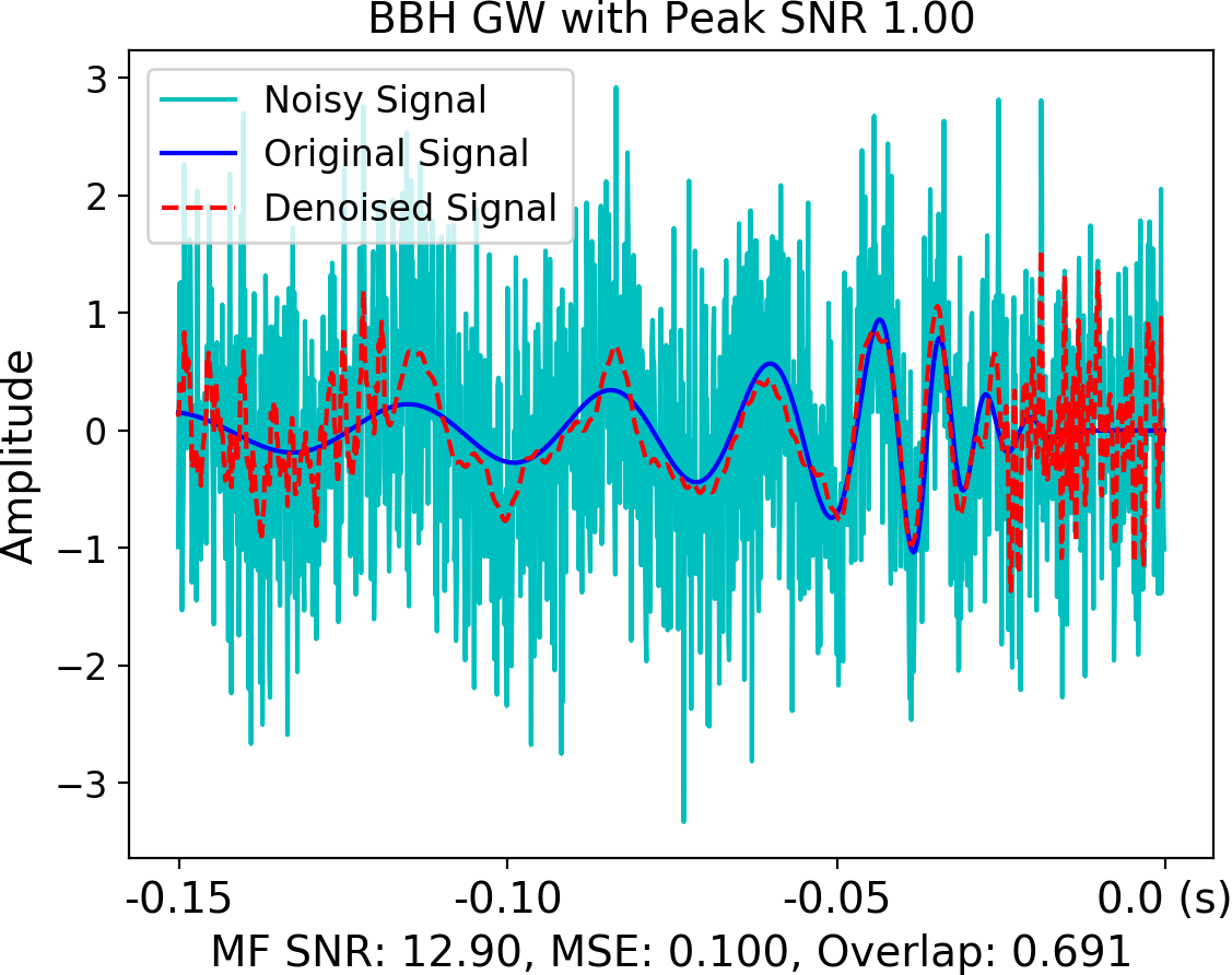
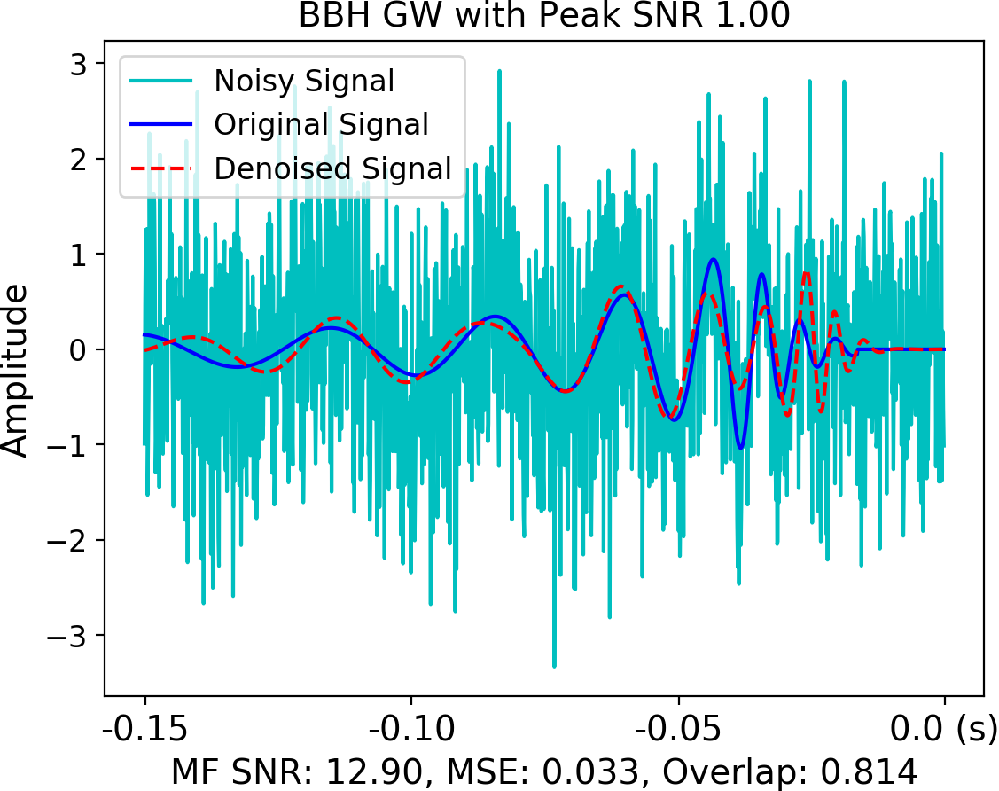
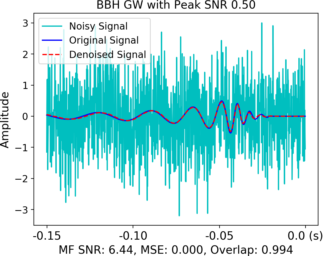
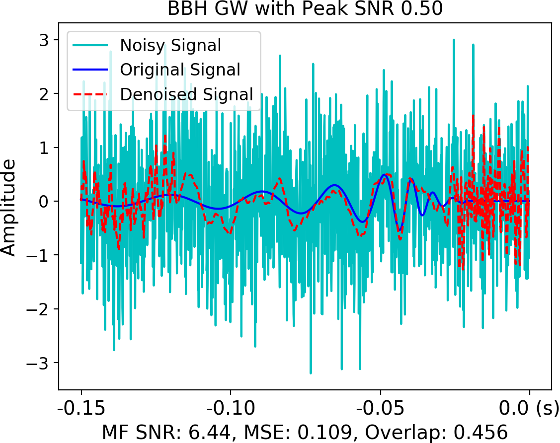
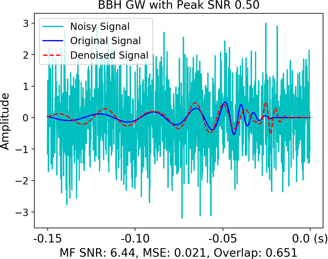
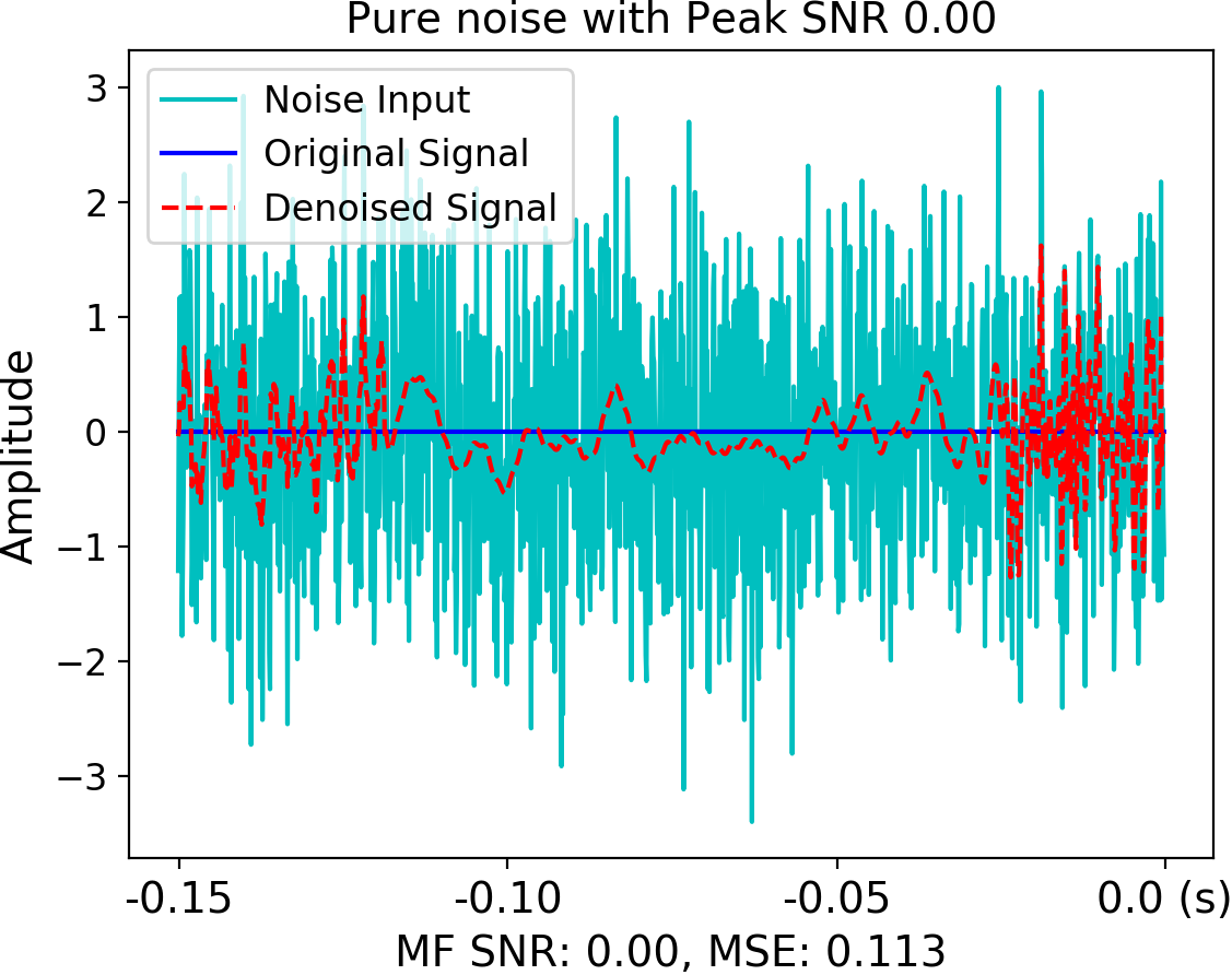
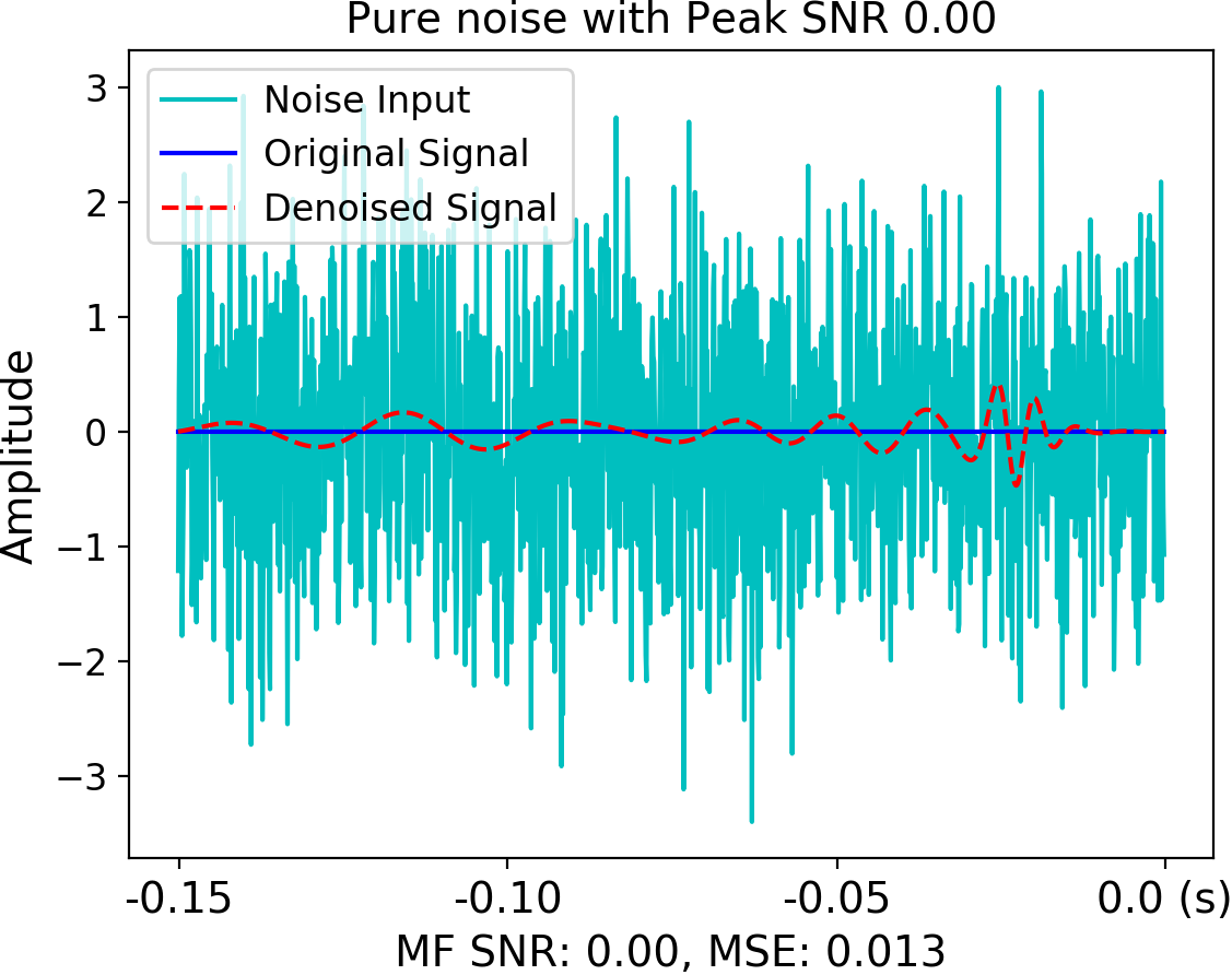
In FIG 2, we show results with PCA, dictionary learning, and SMTDAE, on the test set signals embedded in real LIGO noise. Note that our model was only trained with white Gaussian noise. We show that after training at different SNRs, our model outperforms PCA and dictionary learning in terms of the MSE and Overlap in the presence of real LIGO noise. In addition, our model is able to return a flat output of zeros when the inputs are either pure Gaussian noise or non-Gaussian, non stationary LIGO noise. In terms of computational performance, PCA takes on average two minutes to denoise 1s of input data. In stark contrast, applying our SMTDAE model with a GPU, takes on average less than 100 milliseconds to process 1s of input data.

V Conclusion

We have introduced SMTDAE, a new non-linear algorithm to denoise GW signals which combines a DAE with an RNN architecture using unsupervised learning. When the input data is pure noise, the output of the SMTDAE is close to zero. We have shown that the new approach is more accurate than PCA and dictionary learning methods at recovering GW signals in real LIGO noise, especially at low SNR, and is significantly more computationally efficient than the latter. More importantly, although our model was trained only with additive white Gaussian noise, SMTDAE achieves excellent performance even when the input signals are embedded in real LIGO noise, which is non-Gaussian and non-stationary. This indicates SMTDAE will be able to automatically deal with changes in noise distributions, without retraining, which will occur in the future as the GW detectors undergo modifications to attain design sensitivity.

We have also applied SMTDAE to denoise new classes of GW signals from eccentric binary black hole mergers, simulated with the Einstein Toolkit Löffler et al. (2012), injected into real LIGO noise, and found that we could recover them well even though we only used non-spinning, quasi-circular BBH waveforms for training. This indicates that our denoising method can generalize to new types of signals beyond the training data. We will provide detailed results on denoising different classes of eccentric and spin-precessing binaries as well as supernovae in a subsequent extended article. The encoder in SMTDAE may be used as a feature extractor for unsupervised clustering algorithms George et al. (2017b). Coherent GW searches may be carried out by comparing the output of SMTDAE across multiple detectors or by providing multi-detector inputs to the model. Denoising may also be combined with the Deep Filtering technique George and Huerta (2016, 2017b) for improving the performance of signal detection and parameter estimation of GW signals at low SNR, in the future. We will explore the application of this algorithm to help detect GW signals in real discovery campaigns with the ground-based detectors such as LIGO and Virgo.

References

- LeCun et al. (2015) Y. LeCun, Y. Bengio, and G. Hinton, Nature 521, 436 (2015).
- George and Huerta (2016) D. George and E. A. Huerta, ArXiv e-prints (2016), arXiv:1701.00008 [astro-ph.IM] .
- George and Huerta (2017a) D. George and E. A. Huerta, ArXiv e-prints (2017a), arXiv:1711.03121 [gr-qc] .
- Powell et al. (2015) J. Powell, D. Trifirò, E. Cuoco, I. S. Heng, and M. Cavaglià, Classical and Quantum Gravity 32, 215012 (2015), arXiv:1505.01299 [astro-ph.IM] .
- Powell et al. (2016) J. Powell, A. Torres-Forné, R. Lynch, D. Trifirò, E. Cuoco, M. Cavaglià, I. S. Heng, and J. A. Font, ArXiv e-prints (2016), arXiv:1609.06262 [astro-ph.IM] .
- Zevin et al. (2016) M. Zevin, S. Coughlin, S. Bahaadini, E. Besler, N. Rohani, S. Allen, M. Cabero, K. Crowston, A. Katsaggelos, S. Larson, T. K. Lee, C. Lintott, T. Littenberg, A. Lundgren, C. Oesterlund, J. Smith, L. Trouille, and V. Kalogera, ArXiv e-prints (2016), arXiv:1611.04596 [gr-qc] .
- George et al. (2017a) D. George, H. Shen, and E. A. Huerta, ArXiv e-prints (2017a), arXiv:1706.07446 [gr-qc] .
- George et al. (2017b) D. George, H. Shen, and E. A. Huerta, ArXiv e-prints (2017b), arXiv:1711.07468 [astro-ph.IM] .
- Huerta et al. (2017) E. A. Huerta, C. J. Moore, P. Kumar, D. George, A. J. K. Chua, R. Haas, E. Wessel, D. Johnson, D. Glennon, A. Rebei, A. M. Holgado, J. R. Gair, and H. P. Pfeiffer, ArXiv e-prints (2017), arXiv:1711.06276 [gr-qc] .
- Torres et al. (2015) A. Torres, A. Marquina, J. A. Font, and J. M. Ibáñez, in Gravitational Wave Astrophysics (Springer, 2015) pp. 289–294.
- Torres et al. (2014) A. Torres, A. Marquina, J. A. Font, and J. M. Ibáñez, Phys. Rev. D 90, 084029 (2014).
- Torres et al. (2016a) A. Torres, A. Marquina, J. A. Font, and J. M. Ibáñez, “Denoising of gravitational wave signal GW150914 via total variation methods,” (2016a), arXiv:1602.06833 .
- Jolliffe (2002) I. Jolliffe, Principal Component Analysis (Wiley Online Library, 2002).
- Anderson (2003) T. W. Anderson, An Introduction to Multivariate Statistical Analysis (Wiley New York, 2003).
- Mairal et al. (2009a) J. Mairal, F. Bach, J. Ponce, and G. Sapiro, in Proceedings of the 26th Annual International Conference on Machine Learning, ICML ’09 (ACM, New York, NY, USA, 2009) pp. 689–696.
- Hawe et al. (2013) S. Hawe, M. Seibert, and M. Kleinsteuber, in Proceedings of the 2013 IEEE Conference on Computer Vision and Pattern Recognition, CVPR ’13 (IEEE Computer Society, Washington, DC, USA, 2013) pp. 438–445.
- Mairal et al. (2009b) J. Mairal, J. Ponce, G. Sapiro, A. Zisserman, and F. Bach, in Advances in Neural Information Processing Systems 21, edited by D. Koller, D. Schuurmans, Y. Bengio, and L. Bottou (Curran Associates, Inc., 2009) pp. 1033–1040.
- Aharon et al. (2006) M. Aharon, M. Elad, and A. Bruckstein, IEEE TRANSACTIONS ON SIGNAL PROCESSING 54, 4311 (2006).
- Baraniuk et al. (2010) R. G. Baraniuk, E. Candes, M. Elad, and Y. Ma, Proc. IEEE 98 (2010).
- Gribonval and Nielsen (2006) R. Gribonval and M. Nielsen, Signal Processing 86 (2006).
- Beck and Teboulle (2009) A. Beck and M. Teboulle, SIAM journal on imaging sciences 2, 183 (2009).
- Owen and Sathyaprakash (1999) B. J. Owen and B. S. Sathyaprakash, Phys. Rev. D 60, 022002 (1999).
- Torres et al. (2016b) A. Torres, A. Marquina, J. A. Font, and J. M. Ibáñez, Phys. Rev. D 94, 124040 (2016b).
- Chainais (2012) P. Chainais, in Machine Learning for Signal Processing (MLSP), 2012 IEEE International Workshop on (IEEE, 2012) pp. 1–6.
- Giryes and Elad (2014) R. Giryes and M. Elad, IEEE Transactions on Image Processing 23, 5057 (2014).
- Maas et al. (2012) A. L. Maas, Q. V. Le, T. M. O’Neil, O. Vinyals, P. Nguyen, and A. Y. Ng, in INTERSPEECH 2012, 13th Annual Conference of the International Speech Communication Association, Portland, Oregon, USA, September 9-13, 2012 (2012) pp. 22–25.
- Graves et al. (2013) A. Graves, A. Mohamed, and G. Hinton, “Speech recognition with deep recurrent neural networks,” (2013), arXiv:1303.5778 .
- Arik et al. (2017) S. O. Arik, C. M., A. Coates, G. Diamos, A. Gibiansky, Y. Kang, X. Li, J. Miller, A. Ng, J. Raiman, S. Sengupta, and M. Shoeybi, “Deep voice: Real-time neural text-to-speech,” (2017), arXiv:1702.07825 .
- Zhang et al. (2017) Z. Zhang, J. Geiger, J. Pohjalainen, A. E. Mousa, W. Jin, and B. Schuller, “Deep learning for environmentally robust speech recognition: An overview of recent developments,” (2017), arXiv:1705.10874 .
- Sutskever et al. (2014) I. Sutskever, O. Vinyals, and Q. V. Le, in Advances in neural information processing systems (2014) pp. 3104–3112.
- Graves and Schmidhuber (2009) A. Graves and J. Schmidhuber, in Advances in neural information processing systems (2009) pp. 545–552.
- Bengio et al. (2013) Y. Bengio, L. Yao, G. Alain, and P. Vincent, “Generalized Denoising Auto Encoders as Generative Models,” (2013), arXiv:1305.6663 .
- Vincent et al. (2008) P. Vincent, H. Larochelle, Y. Bengio, and P. A. Manzagol, in Proceedings of the 25th International Conference on Machine Learning, ICML ’08 (ACM, New York, NY, USA, 2008) pp. 1096–1103.
- Vincent et al. (2010) P. Vincent, H. Larochelle, I. Lajoie, Y. Bengio, and P. A. Manzagol, J. Mach. Learn. Res. 11, 3371 (2010).
- Usman et al. (2016) S. A. Usman et al., Class. Quant. Grav. 33, 215004 (2016), arXiv:1508.02357 [gr-qc] .
- Dal Canton et al. (2014) T. Dal Canton et al., Phys. Rev. D90, 082004 (2014), arXiv:1405.6731 [gr-qc] .
- Hochreiter and Schmidhuber (1997) S. Hochreiter and J. Schmidhuber, Neural computation 9, 1735 (1997).
- Mukund et al. (2017) N. Mukund, S. Thakur, S. Abraham, A. K. Aniyan, S. Mitra, N. S. Philip, K. Vaghmare, and D. P. Acharjya, “Information Retrieval and Recommendation System for Astronomical Observatories,” (2017), arXiv:1710.05350 .
- Shen et al. (2017) H. Shen, D. George, E. A. Huerta, and Z. Zhao, ArXiv e-prints (2017).
- Bohé et al. (2017) A. Bohé, L. Shao, A. Taracchini, A. Buonanno, S. Babak, I. W. Harry, I. Hinder, S. Ossokine, M. Pürrer, V. Raymond, T. Chu, H. Fong, P. Kumar, H. P. Pfeiffer, M. Boyle, D. A. Hemberger, L. E. Kidder, G. Lovelace, M. A. Scheel, and B. Szilágyi, Phys. Rev. D 95, 044028 (2017), arXiv:1611.03703 [gr-qc] .
- (41) LSC, “LSC Algorithm Library software packages lal, lalwrapper, and lalapps,” http://www.lsc-group.phys.uwm.edu/lal.
- Shoemaker (2010) D. Shoemaker, “Advanced LIGO anticipated sensitivity curves,” (2010).
- Abbott et al. (2016a) B. P. Abbott, R. Abbott, T. D. Abbott, M. R. Abernathy, F. Acernese, K. Ackley, C. Adams, T. Adams, P. Addesso, R. X. Adhikari, and et al., Physical Review Letters 116, 061102 (2016a), arXiv:1602.03837 [gr-qc] .
- Abbott et al. (2016b) B. P. Abbott, R. Abbott, T. D. Abbott, M. R. Abernathy, F. Acernese, K. Ackley, C. Adams, T. Adams, P. Addesso, R. X. Adhikari, and et al., Physical Review Letters 116, 241103 (2016b), arXiv:1606.04855 [gr-qc] .
- Abbott et al. (2017a) B. P. Abbott, R. Abbott, T. D. Abbott, M. R. Abernathy, F. Acernese, K. Ackley, C. Adams, T. Adams, P. Addesso, R. X. Adhikari, et al., Physical Review Letters 118, 221101 (2017a).
- Abbott et al. (2017b) B. P. Abbott, R. Abbott, T. D. Abbott, F. Acernese, K. Ackley, C. Adams, T. Adams, P. Addesso, R. X. Adhikari, V. B. Adya, and et al., Physical Review Letters 119, 141101 (2017b), arXiv:1709.09660 [gr-qc] .
- Weiss et al. (2016) K. Weiss, T. M. Khoshgoftaar, and D. Wang, Journal of Big Data 3, 9 (2016).
- Bengio et al. (2009) Y. Bengio, J. Louradour, R. Collobert, and J. Weston, in Proceedings of the 26th annual international conference on machine learning (ACM, 2009) pp. 41–48.
- Abadi et al. (2016) M. Abadi, A. Agarwal, P. Barham, E. Brevdo, Z. Chen, C. Citro, G. S. Corrado, A. Davis, J. Dean, M. Devin, et al., “TensorFlow: Large-Scale Machine Learning on Heterogeneous Distributed Systems,” (2016), arXiv:1603.04467 .
- Mairal et al. (2014) J. Mairal, F. Bach, and J. Ponce, “Sparse modeling for image and vision processing,” (2014), arXiv:1411.3230 .
- Löffler et al. (2012) F. Löffler, J. Faber, E. Bentivegna, T. Bode, P. Diener, R. Haas, I. Hinder, B. C. Mundim, C. D. Ott, E. Schnetter, G. Allen, M. Campanelli, and P. Laguna, Classical and Quantum Gravity 29, 115001 (2012), arXiv:1111.3344 [gr-qc] .
- George and Huerta (2017b) D. George and E. A. Huerta, ArXiv e-prints (2017b), arXiv:1711.07966 [gr-qc] .