Laura⁺⁺ : a Dalitz plot fitter

John Back, Tim Gershon, Paul Harrison, Thomas Latham,

Daniel O’Hanlon, Wenbin Qian

Department of Physics, University of Warwick, Coventry, United Kingdom

Pablo del Amo Sanchez

LAPP, Université Savoie Mont-Blanc, CNRS/IN2P3, Annecy-Le-Vieux, France

Daniel Craik

Massachusetts Institute of Technology, Cambridge, United States of America

Jelena Ilic

STFC Rutherford Appleton Laboratory, Didcot, United Kingdom

Juan Martin Otalora Goicochea

Universidade Federal do Rio de Janeiro (UFRJ), Rio de Janeiro, Brazil

Eugenia Puccio

Stanford University, Stanford, United States of America

Rafael Silva Coutinho

Physik-Institut, Universität Zürich, Zürich, Switzerland

Mark Whitehead

European Organization for Nuclear Research (CERN), Geneva, Switzerland

The Dalitz plot analysis technique has become an increasingly important method in heavy flavour physics. The Laura⁺⁺ fitter has been developed as a flexible tool that can be used for Dalitz plot analyses in different experimental environments. Explicitly designed for three-body decays of heavy-flavoured mesons to spinless final state particles, it is optimised in order to describe all possible resonant or nonresonant contributions, and to accommodate possible $C\!P$ violation effects.

1 Introduction

Decays of unstable heavy particles to multibody final states can in general occur through several different intermediate resonances. Each decay channel can be represented quantum-mechanically by an amplitude, and the total density of decays across the phase space is represented by the square of the coherent sum of all contributing amplitudes. Interference effects can lead to excesses or deficits of decays in regions of phase space where different resonances overlap. Investigations of such dynamical effects in multibody decays are of great interest to test the Standard Model of particle physics and to investigate resonant structures.

The Dalitz plot (DP) [1, 2] was introduced originally to describe the phase space of ${{K}^{0}_{\rm\scriptscriptstyle L}}\rightarrow\pi\pi\pi$ decays, but is relevant for the decay of any spin-zero particle to three spin-zero particles, $P\rightarrow d_{1}d_{2}d_{3}$. In such a case, energy and momentum conservation give

$$m_{P}^{2}+m_{d_{1}}^{2}+m_{d_{2}}^{2}+m_{d_{3}}^{2}=m^{2}(d_{1}d_{2})+m^{2}(d_{2}d_{3})+m^{2}(d_{3}d_{1})\,,$$ (1)

where $m(d_{i}d_{j})$ is the invariant mass obtained from the two-body combination of the $d_{i}$ and $d_{j}$ four momenta. Consequently, assuming that the masses of $P$, $d_{1}$, $d_{2}$ and $d_{3}$ are all known, any two of the $m^{2}(d_{i}d_{j})$ values — subsequently referred to as Dalitz-plot variables — are sufficient to describe fully the kinematics of the decay in the $P$ rest frame. This can also be shown by considering that the 12 degrees of freedom corresponding to the four-momenta of the three final-state particles are accounted for by two DP variables, the three $d_{i}$ masses, four constraints due to energy–momentum conservation in the $P\rightarrow d_{1}d_{2}d_{3}$ decay, and three co-ordinates describing a direction in space which carries no physical information about the decay since all particles involved have zero spin.

A Dalitz plot is then the visualisation of the phase space of a particular three-body decay in terms of the two DP variables. Analysis of the distribution of decays across a DP can reveal information about the underlying dynamics of the particular three-body decay, since the differential rate is

$$d\Gamma=\frac{1}{(2\pi)^{3}}\frac{1}{32\,m_{P}^{3}}\left|{\cal A}\right|^{2}dm^{2}(d_{1}d_{3})\,dm^{2}(d_{2}d_{3})\,,$$ (2)

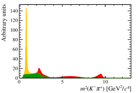
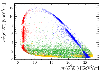
where ${\cal A}$ is the amplitude for the three-body decay. Thus, any deviation from a uniform distribution is due to the dynamical structure of the amplitude. Examples of the kinematic boundaries of a DP, and of resonant structures that may appear in this kind of decay, are shown in Fig. 1.

Figure 1: (Top left) kinematic boundaries of the three-body phase space for the decay ${{B}^{0}_{s}}\rightarrow{{\kern 1.99997pt\overline{\kern-1.99997ptD}{}}{}^{0}}{{K}^{-}}{{\pi}^{+}}$. The insets indicate the configuration of the final-state particle momenta in the parent rest frame at various different DP positions. (Top right) examples of the resonances which may appear in the Dalitz plot for this decay: (red) ${D}^{*}_{s2}(2573)^{-}$, (orange) ${K}^{*}(892)^{0}$, (green) ${K}{\pi}$ S-wave. (Bottom) projections of this DP onto the squares of the invariant masses (from left to right): $m^{2}_{{{\kern 1.39998pt\overline{\kern-1.39998ptD}{}}{}^{0}}{{\pi}^{+}}}$, $m^{2}_{{{\kern 1.39998pt\overline{\kern-1.39998ptD}{}}{}^{0}}{{K}^{-}}}$, $m^{2}_{{{K}^{-}}{{\pi}^{+}}}$.

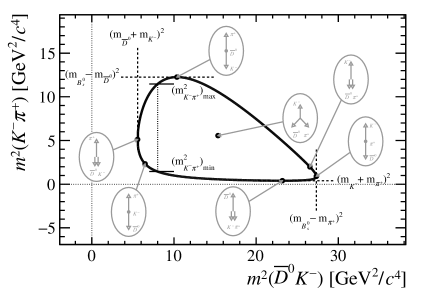
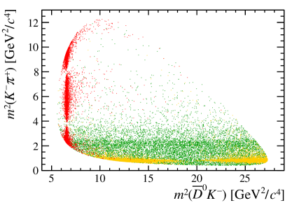
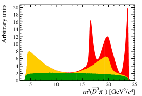
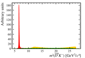
The Dalitz-plot analysis technique, usually implemented with model-dependent descriptions of the amplitudes involved, has been used to understand hadronic effects in, for example, the $\pi^{0}\pi^{0}\pi^{0}$ system produced in $p\bar{p}$ annihilation [3]. Recently, it has also been used to study three-body $\eta_{c}$ decays [4, 5]. However, DP analyses have become particularly popular to study multibody decays of the heavy-flavoured $D$ and $B$ mesons. Not only do the relatively large masses of these particles provide a broad kinematic range in which resonant structures can be studied but, since the decays are mediated by the weak interaction, there may be $C\!P$-violating differences between the DP distributions for particle and antiparticle. Studying these differences can test the Standard Model mechanism for $C\!P$ violation: if the asymmetries are not consistent with originating from the single complex phase in the Cabibbo-Kobayashi-Maskawa (CKM) quark mixing matrix [6, 7] then contributions beyond the Standard Model must be present.

Until around the year 2000, most DP analyses of charm decays were focussed on understanding hadronic structures at low $\pi\pi$ or $K\pi$ mass. In particular, pioneering analyses of $D\rightarrow K\pi\pi$ decays were carried out by experiments such as MARK-II, MARK-III, E687, ARGUS, E691 and CLEO [8, 9, 10, 11, 12, 13]. These analyses revealed the existence of a broad structure in the $K\pi$ S-wave that could not be well described with a Breit–Wigner lineshape. In later analyses, it was shown that this contribution could be modelled in a quasi-model-independent way, in which the partial wave is fitted using splines to describe the magnitude and phase as a function of $m(K\pi)$ [14]. Subsequent uses of this approach include further studies of the $K\pi$ S-wave [15, 16, 17, 5] as well as the ${{K}^{+}}{{K}^{-}}$ [18] and ${{\pi}^{+}}{{\pi}^{-}}$ [19] S-waves, in various processes. Similarly, DP analyses of decays such as ${{D}^{+}}\rightarrow{{\pi}^{+}}{{\pi}^{+}}{{\pi}^{-}}$ [20, 21, 22, 23] indicated the existence of a broad low-mass $\pi\pi$ S-wave known as the $\sigma$ pole [24].

With the advent of the $e^{+}e^{-}$ $B$-factory experiments, BaBar [25, 26] and Belle [27], DP analyses of $B$ meson decays became feasible. The method was used to obtain insights into charm resonances through analyses of ${{{B}^{+}}}\rightarrow{{D}^{-}}{{\pi}^{+}}{{\pi}^{+}}$ [28, 29] and ${{B}^{0}}\rightarrow{{\kern 1.99997pt\overline{\kern-1.99997ptD}{}}{}^{0}}{{\pi}^{+}}{{\pi}^{-}}$ [30, 31] decays. Studies of $B$ meson decays to final states without any charm or charmonium particles also became possible [32, 33, 34]. Once baseline DP models were established, it was then possible to search for $C\!P$ violation effects, with results including the first evidence for $C\!P$ violation in the ${{{B}^{+}}}\rightarrow\rho(770)^{0}{{K}^{+}}$ decay [35, 36]. Moreover, analyses that accounted for possible dependence of the $C\!P$ violation effect with decay time as well as with DP position were carried out for both $D$ [37, 38] and $B$ decays [39, 40, 41, 42, 43, 44, 45, 46].

With the availability of increasingly large data samples at these experiments and, more recently, at the Large Hadron Collider experiments (in particular, LHCb [47]), more detailed studies of these and similar decays become possible. In addition, many ideas for DP analyses have been proposed, since they provide interesting possibilities to provide insight into hadronic structures, to measure $C\!P$ violation effects and to test the Standard Model. These include methods to determine the angles $\alpha$, $\beta$ and $\gamma$ of the CKM Unitarity Triangle with low theoretical uncertainty from, respectively ${{B}^{0}}\rightarrow{{\pi}^{+}}{{\pi}^{-}}{{\pi}^{0}}$ [48], ${{B}^{0}}\rightarrow D{{\pi}^{+}}{{\pi}^{-}}$ [49, 50] and ${{B}^{0}}\rightarrow D{{K}^{+}}{{\pi}^{-}}$ decays [51, 52], among many other potential analyses.

Thus, it has become increasingly important to have a publicly available Dalitz-plot analysis package that is flexible enough both to be used in a range of experimental environments and to describe many possible different decays and types of analyses. Such a package should be well validated and have excellent performance characteristics, in particular in terms of speed since complicated amplitude fits can otherwise have unacceptable CPU requirements. This motivated the creation, and ongoing development, of the Laura⁺⁺ package, which is described in the remainder of the paper. Laura⁺⁺ is written in the C++ programming language and is intended to be as close as possible to being a standalone package, with a sole external dependency on the Root package [53]. In particular, Root is used to handle data file input/output, histogrammed quantities, and the minimisation of negative log-likelihood functions with Minuit [54]. Further documentation and code releases (distributed under the Apache License, Version 2.0 [55]) are available from

http://laura.hepforge.org/   .

The description of the software given in this paper corresponds to that released in Laura⁺⁺ version v3r4.

In Sec. 2, a brief summary of the Dalitz-plot analysis formalism is given, and the conventions used in Laura⁺⁺ are set out. Section 3 describes effects that must also be taken into account when performing an experimental analysis. Sections 4, 5 and 6 then contain discussions of, respectively, the implementation of the signal model, efficiency and resolution effects, and the background components in Laura⁺⁺, including explicit classes and methods with high-level details given in Appendices. These elements are then put together in Sec. 7, where the overall work flow in Laura⁺⁺ is described. The performance of the software is discussed in Sec. 8, ongoing and planned future developments are briefly mentioned in Sec. 9, and a summary is given in Sec. 10.

2 Dalitz-plot analysis formalism

Given two variables that describe the Dalitz plot of the $P\rightarrow d_{1}d_{2}d_{3}$ decay, all other kinematic quantities can be uniquely determined for fixed initial- and final-state (subsequently referred to as parent and daughter) particle masses. The convention adopted in Laura⁺⁺ is that the DP is described in terms of $m^{2}_{13}\equiv m^{2}(d_{1}d_{3})$ and $m^{2}_{23}\equiv m^{2}(d_{2}d_{3})$. Hence, these two variables are required to be present in any input data provided to Laura⁺⁺.

The description of the complex amplitude is based on the isobar model [56, 57, 58], which describes the total amplitude as a coherent sum of $N$ amplitudes from resonant or nonresonant intermediate processes. This means that the total amplitude is given by

$${\cal A}\left(m^{2}_{13},m^{2}_{23}\right)=\sum_{j=1}^{N}c_{j}F_{j}\left(m^{2}_{13},m^{2}_{23}\right)\,,$$ (3)

where $c_{j}$ are complex coefficients, discussed further in Sec. 4.5, giving the relative contribution of decay channel $j$. There are several different choices used in the literature to express the resonance dynamics contained within the $F_{j}\left(m^{2}_{13},m^{2}_{23}\right)$ terms. Here, one common approach, which is the default in Laura⁺⁺, is outlined; other possibilities are discussed in Appendices A and B. For a resonance in $m_{13}$, the dynamics can be written as

$$F\left(m^{2}_{13},m^{2}_{23}\right)={\cal N}\times R\left(m_{13}\right)\times T(\vec{p},\vec{q})\times X(|\vec{p}|\,r^{P}_{\rm BW})\times X(|\vec{q}|\,r^{R}_{\rm BW})\,,$$ (4)

where the functions $R$ and $T$ describe the invariant mass and angular dependence of the amplitude, the $X$ functions are form factors, and ${\cal N}$ is a normalisation constant. In Eq. (4) only the kinematic — i.e. DP — dependence has been specified; the functions may also depend on properties of the resonance such as mass, width and spin. The arguments $\vec{q}$ and $\vec{p}$ are the momentum of one of the resonance decay products ($d_{3}$ in this case, see Sec. 2.4 for further information) and that of the so-called “bachelor” particle (i.e. the particle not associated with the decay of the resonance; $d_{2}$ in this case), both evaluated in the rest frame of the resonance. The parameters $r^{P}_{\rm BW}$ and $r^{R}_{\rm BW}$ are characteristic meson radii described below. The resonance dynamics are normalised in Laura⁺⁺ such that the integral over the DP of the squared magnitude of each term is unity

$$\int\!\!\int_{\rm DP}\,\left|F_{j}\left(m^{2}_{13},m^{2}_{23}\right)\right|^{2}\,dm^{2}_{13}\,dm^{2}_{23}=1\,.$$ (5)

Although not strictly necessary, as only the total probability density function (PDF) needs to be normalised, this allows a meaningful comparison of the values of the $c_{j}$ coefficients.

2.1 Resonance lineshapes

In Eq. (4), the function $R\left(m_{13}\right)$ is the resonance mass term. The detailed forms for all available shapes in Laura⁺⁺ are given in App. A. Here the most commonly used relativistic Breit–Wigner (RBW) lineshape is given as an example

$$R(m)=\frac{1}{(m_{0}^{2}-m^{2})-i\,m_{0}\Gamma(m)}\,,$$ (6)

where $m_{0}$ is the nominal mass of the resonance and the dependence of the decay width of the resonance on $m$ is given by

$$\Gamma(m)=\Gamma_{0}\left(\frac{q}{q_{0}}\right)^{2L+1}\left(\frac{m_{0}}{m}\right)X^{2}(q\,r^{R}_{\rm BW})\,,$$ (7)

where $\Gamma_{0}$ is the nominal width of the resonance and $q_{0}$ denotes the value of $q$ when $m=m_{0}$. In Eq. (7), $L$ is the orbital angular momentum between the resonance daughters. Note that since all the initial- and final-state particles have zero spin, this quantity is the same as the spin of the resonance and is also the same as the orbital angular momentum between the resonance and the bachelor.

It is relevant to note that Eq. (6) can be written

$$m_{0}\Gamma(m)R(m)=\frac{m_{0}\Gamma(m)}{(m_{0}^{2}-m^{2})-i\,m_{0}\Gamma(m)}\equiv\sin\phi\exp{i\phi}\,,$$ (8)

where $\tan\phi=\frac{m_{0}\Gamma(m)}{m_{0}^{2}-m^{2}}$. This shows the characteristic phase rotation of a resonance as $m^{2}$ increases from far below to far above $m_{0}^{2}$.

2.2 Angular distributions and Blatt–Weisskopf form factors

Using the Zemach tensor formalism [59, 60], the angular probability distribution terms $T(\vec{p},\vec{q})$ are given by

$$L=0\ :\ T(\vec{p},\vec{q}) = \phantom{-}\,1\,,$$ (9)

$$L=1\ :\ T(\vec{p},\vec{q}) = -\,2\,\vec{p}\cdot\vec{q}\,,$$ (10)

$$L=2\ :\ T(\vec{p},\vec{q}) = \phantom{-}\,\frac{4}{3}\left[3(\vec{p}\cdot\vec{q}\,)^{2}-(p\,q)^{2}\right]\,,$$ (11)

$$L=3\ :\ T(\vec{p},\vec{q}) = -\,\frac{24}{15}\left[5(\vec{p}\cdot\vec{q}\,)^{3}-3(\vec{p}\cdot\vec{q}\,)(p\,q)^{2}\right]\,,$$ (12)

$$L=4\ :\ T(\vec{p},\vec{q}) = \phantom{-}\,\frac{16}{35}\left[35(\vec{p}\cdot\vec{q}\,)^{4}-30(\vec{p}\cdot\vec{q}\,)^{2}(p\,q)^{2}+3(p\,q)^{4}\right]\,,$$ (13)

$$L=5\ :\ T(\vec{p},\vec{q}) = -\,\frac{32}{63}\left[63(\vec{p}\cdot\vec{q}\,)^{5}-70(\vec{p}\cdot\vec{q}\,)^{3}(p\,q)^{2}+15(\vec{p}\cdot\vec{q}\,)(p\,q)^{4}\right]~{},$$ (14)

where $q\equiv|\vec{q}\,|$ and $p\equiv|\vec{p}\,|$. These have the form of the Legendre polynomials $P_{L}(\cos\theta)$, where $\theta$ is the “helicity” angle between $\vec{p}$ and $\vec{q}$, multiplied by the appropriate power of $-2\,p\,q$. These factors act to suppress the amplitude at low values of the break-up momentum in either the decay of the parent or the resonance — the so-called “angular momentum barrier”. However, these factors on their own would cause the amplitude to continue to grow with increasing break-up momentum even once the barrier was exceeded. The terms $X(z)$, where $z=p\,r^{P}_{\rm BW}$ or $q\,r^{R}_{\rm BW}$, are Blatt–Weisskopf form factors [61], which act to cancel this behaviour once above the barrier. They are given by

$$L=0\ :\ X(z) = 1\,,$$ (15)

$$L=1\ :\ X(z) = \sqrt{\frac{1+z_{0}^{2}}{1+z^{2}}}\,,$$ (16)

$$L=2\ :\ X(z) = \sqrt{\frac{z_{0}^{4}+3z_{0}^{2}+9}{z^{4}+3z^{2}+9}}\,,$$ (17)

$$L=3\ :\ X(z) = \sqrt{\frac{z_{0}^{6}+6z_{0}^{4}+45z_{0}^{2}+225}{z^{6}+6z^{4}+45z^{2}+225}}\,,$$ (18)

$$L=4\ :\ X(z) = \sqrt{\frac{z_{0}^{8}+10z_{0}^{6}+135z_{0}^{4}+1575z_{0}^{2}+11025}{z^{8}+10z^{6}+135z^{4}+1575z^{2}+11025}}\,,$$ (19)

$$L=5\ :\ X(z) = \sqrt{\frac{z_{0}^{10}+15z_{0}^{8}+315z_{0}^{6}+6300z_{0}^{4}+99225z_{0}^{2}+893025}{z^{10}+15z^{8}+315z^{6}+6300z^{4}+99225z^{2}+893025}}\,,$$ (20)

where $z_{0}$ represents the value of $z$ when $m=m_{0}$. The radius of the barrier, denoted $r^{P}_{\rm BW}$ or $r^{R}_{\rm BW}$ where the superscript indicates that the parameter is associated with either the parent or resonance in the decay chain, is usually taken to be $4.0\mathrm{\,Ge\kern-1.00006ptV}^{-1}\approx 0.8\rm\,fm$ [34]. Alternative descriptions of the angular distributions and Blatt–Weisskopf form factors are given in App. B.

2.3 Fit fractions

In the absence of any reconstruction effects, the DP PDF would be

$${\cal{P}}_{\rm phys}\left(m^{2}_{13},m^{2}_{23}\right)=\frac{\left|{\cal A}\left(m^{2}_{13},m^{2}_{23}\right)\right|^{2}}{\int\!\!\int_{\rm DP}~{}{\left|{\cal A}\left(m^{2}_{13},m^{2}_{23}\right)\right|^{2}}~{}dm^{2}_{13}\,dm^{2}_{23}}\,.$$ (21)

In a real experiment, the variation of the efficiency across the DP and the contamination from background processes must be taken into account; these details are discussed in Sections 3, 5 and 6.

Typically, the primary results — i.e. the values obtained directly in the fit to data — of a DP analysis include the complex amplitude coefficients, given by $c_{j}$ in Eq. (3), that describe the relative contributions of each intermediate process. These results are dependent on a number of factors, including the amplitude formalism, choice of normalisation and phase convention used in each DP analysis. This makes it difficult to make useful comparisons between complex coefficients obtained from different analyses using different software. Fit fractions provide a convention-independent method to make meaningful comparisons of results from different fits. The fit fraction is defined as the integral of a single decay amplitude squared divided by that of the coherent matrix element squared for the complete DP,

$${\it FF}_{j}=\frac{\int\!\!\int_{\rm DP}\left|c_{j}F_{j}\left(m^{2}_{13},m^{2}_{23}\right)\right|^{2}~{}dm^{2}_{13}\,dm^{2}_{23}}{\int\!\!\int_{\rm DP}\left|{\cal A}\left(m^{2}_{13},m^{2}_{23}\right)\right|^{2}~{}dm^{2}_{13}\,dm^{2}_{23}}\,.$$ (22)

The sum of these fit fractions is not necessarily unity due to the potential presence of net constructive or destructive interference. Such effects can be quantified by defining interference fit fractions (for $i<j$ only) as

$${\it FF}_{ij}=\frac{\int\!\!\int_{\rm DP}2\,{\rm Re}\left[c_{i}c_{j}^{*}F_{i}\left(m^{2}_{13},m^{2}_{23}\right)F_{j}^{*}\left(m^{2}_{13},m^{2}_{23}\right)\right]~{}dm^{2}_{13}\,dm^{2}_{23}}{\int\!\!\int_{\rm DP}\left|{\cal A}\left(m^{2}_{13},m^{2}_{23}\right)\right|^{2}~{}dm^{2}_{13}\,dm^{2}_{23}}\,.$$ (23)

The interference fit fractions describe the net interference between the amplitudes of two intermediate processes. Interference effects between different partial waves in a given two-body combination cancel when integrated over the helicity angle. Therefore, non-zero interference fit fractions should arise only between contributions in the same partial wave of one two-body combination, or between contributions in different two-body combinations. Large interference fit fractions, or equivalently a sum of fit fractions very different from unity, can often be an indication of inadequate modelling of the Dalitz plot.

2.4 Helicity angle convention

In the formalism just described, there is a choice as to which of the two resonance daughters the momentum $\vec{q}$ should be attributed (and hence to attribute the momentum $-\vec{q}$ to the other). This choice, although arbitrary, will affect the values of the measured phases and hence it is important that it is documented to allow comparisons between results. The convention used in Laura⁺⁺ is as follows:

• $\theta_{12}$ is defined as the angle between $d_{1}$ and $d_{3}$ in the rest frame of the $d_{1}$ and $d_{2}$ system, i.e. $\vec{q}$ is the momentum of $d_{1}$;

• $\theta_{23}$ is defined as the angle between $d_{3}$ and $d_{1}$ in the rest frame of the $d_{2}$ and $d_{3}$ system, i.e. $\vec{q}$ is the momentum of $d_{3}$;

• $\theta_{13}$ is defined as the angle between $d_{3}$ and $d_{2}$ in the rest frame of the $d_{1}$ and $d_{3}$ system, i.e. $\vec{q}$ is the momentum of $d_{3}$.

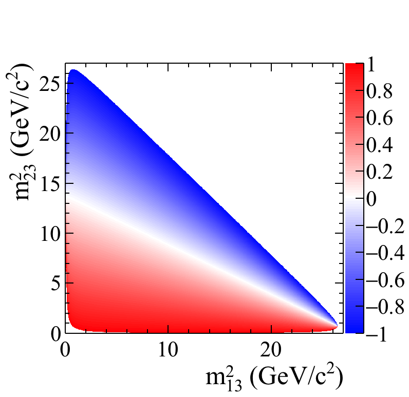
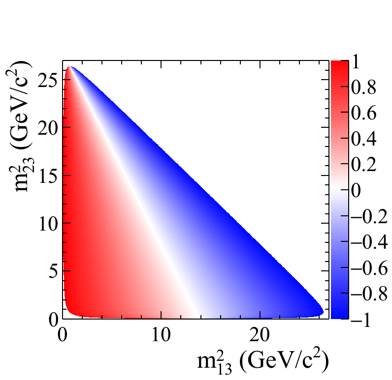
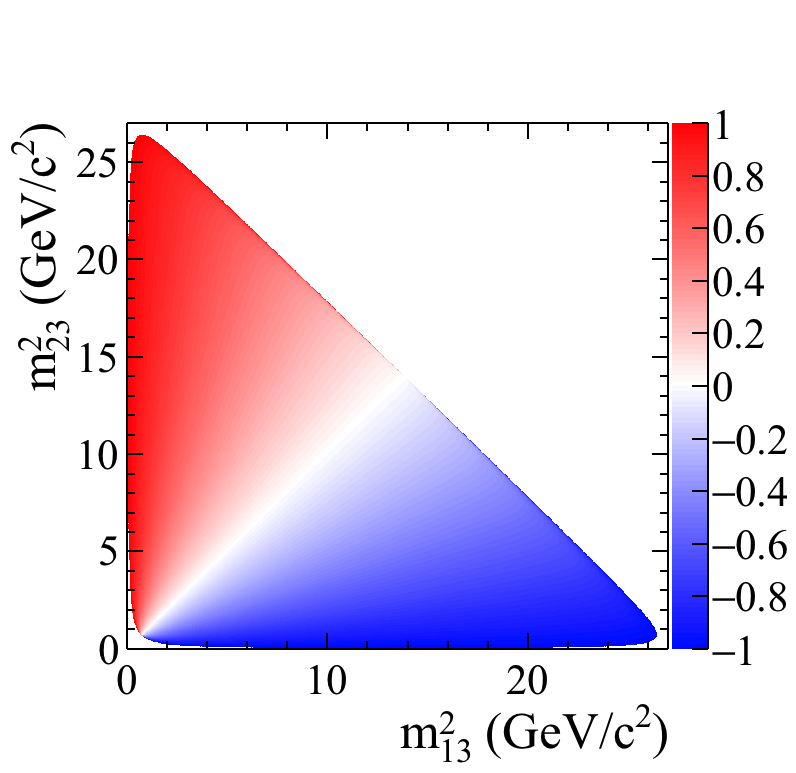
This convention is illustrated in Fig. 2. One important point to note is that it is not a cyclic permutation. Rather it is designed such that for decays where $d_{1}$ and $d_{2}$ are identical particles the formalism is already symmetric under their exchange, as required.

For decays of neutral particles to flavour-conjugate final states containing two charged daughters, e.g. $\kern 1.79993pt\shortstack{{(\rule[2.15277pt]{12.50002pt}{0.51212pt})} \\ [-.7ex] $\kern-1.79993ptB$}{}\rightarrow{{\pi}^{+}}{{\pi}^{-}}{{K}^{0}_{\rm\scriptscriptstyle S}}$, there is a further complication that must be considered. In the example given, if one chooses for the $B$ decay that $d_{1}$ would be ${\pi}^{+}$, $d_{2}$ would be ${\pi}^{-}$ and $d_{3}$ would be ${K}^{0}_{\rm\scriptscriptstyle S}$, one should then define the $\kern 1.79993pt\overline{\kern-1.79993ptB}{}$ decay using the conjugate particles, i.e. $d_{1}$ would be ${\pi}^{-}$, $d_{2}$ would be ${\pi}^{+}$ and $d_{3}$ would be ${K}^{0}_{\rm\scriptscriptstyle S}$. In practice, however, one often has an untagged data sample that contains both $B$ and $\kern 1.79993pt\overline{\kern-1.79993ptB}{}$ decays that are not distinguished and so a single definition of the DP must be used. (Flavour-tagged analyses are discussed in Sec. 9.) Consequently, the amplitude model must account for the incorrect particle assignments for one of the flavours. Due to the choice of convention in Laura⁺⁺ this can be handled in a straightforward manner as long as the self-conjugate particle (the ${K}^{0}_{\rm\scriptscriptstyle S}$ in the example given) is assigned to be $d_{3}$. Under these circumstances, the relation $F\left(m^{2}_{13},m^{2}_{23}\right)={\kern 1.99997pt\overline{\kern-1.99997ptF}{}}\left(m^{2}_{23},m^{2}_{13}\right)$ can be restored simply by multiplying by $-1$ the cosine of the helicity angle $\theta_{12}$ in the amplitude calculations for either the particle or antiparticle decay — we choose to do this for the particle decay (the $B$ decay in the example given). So, in the considered example, a contribution from ${{B}^{0}}\rightarrow\rho(770)^{0}{{K}^{0}_{\rm\scriptscriptstyle S}}$ would have its helicity angle definition inverted with respect to that of ${{\kern 1.79993pt\overline{\kern-1.79993ptB}{}}{}^{0}}\rightarrow\rho(770)^{0}{{K}^{0}_{\rm\scriptscriptstyle S}}$.

Figure 2: Values of the cosine of the helicity angles (left) $\theta_{13}$, (middle) $\theta_{23}$, and (right) $\theta_{12}$ as functions of DP position. The kinematic boundary of this DP corresponds to that for the ${{\kern 1.79993pt\overline{\kern-1.79993ptB}{}}{}^{0}}\rightarrow{{\pi}^{+}}{{\pi}^{-}}{{\pi}^{0}}$ decay.

3 Experimental effects

In order to extract physics results from reconstructed $P\rightarrow d_{1}d_{2}d_{3}$ candidates using real experimental data, several effects need to be taken into account. One major concern will be that any backgrounds that fake the signature of signal decays need to be removed, which is usually done by imposing various selection criteria that exploit differences in the kinematics and topologies between signal and background events.

The effect of applying selection criteria invariably means that the probability of reconstructing signal decays will not be 100% and furthermore could vary as a function of DP position. Along the boundaries, at least one of the daughter particles has low momentum, which typically reduces the reconstruction efficiency compared to decays at or near the DP centre. To account for this effect properly, the signal PDF, originally defined in Eq. (21), needs to be modified to

$${\cal{P}}_{\rm sig}\left(m^{2}_{13},m^{2}_{23}\right)=\frac{\left|{\cal A}\left(m^{2}_{13},m^{2}_{23}\right)\right|^{2}\,\epsilon\left(m^{2}_{13},m^{2}_{23}\right)}{\int\!\!\int_{\rm DP}~{}{\left|{\cal A}\left(m^{2}_{13},m^{2}_{23}\right)\right|^{2}\,\epsilon\left(m^{2}_{13},m^{2}_{23}\right)}~{}dm^{2}_{13}\,dm^{2}_{23}}\,,$$ (24)

where the signal efficiency $\epsilon\left(m^{2}_{13},m^{2}_{23}\right)$ is defined as the fraction of signal decays at the given DP position that are retained after all selection criteria have been applied.

For certain modes, there can be decay channels that can mimic the properties of the signal mode under study. For example, there may be significant backgrounds to the charmless decay ${{{B}^{-}}}\rightarrow{{K}^{-}}{{\pi}^{+}}{{\pi}^{-}}$ from the decay modes ${{{B}^{-}}}\rightarrow{{D}^{0}}{{\pi}^{-}},{{D}^{0}}\rightarrow{{K}^{-}}{{\pi}^{+}}$ or ${{{B}^{-}}}\rightarrow\chi_{c0}{{K}^{-}},\chi_{c0}\rightarrow{{\pi}^{+}}{{\pi}^{-}}$. Such backgrounds can be removed, or at least suppressed, by applying a “veto”, which means excluding candidates that lie within, typically, three to five widths on either side of the mass peak. Alternatively, they can be accounted for within the signal model.

Another issue that needs to be considered is the effect of finite experimental resolution in the determination of the momentum of the parent $P$ and its daughter particles. This leads to imperfect measurements of the invariant mass-squared combinations of the daughters, and also causes uncertainty on the invariant mass of the reconstructed $P$ candidate. To avoid creating a DP with a fuzzy boundary, the mass of $P$ can be fixed to its expected value, with adjustments made to the four-momenta of its daughter particles to ensure momentum–energy conservation. This will in general improve the resolution of the measurement of the DP co-ordinates, however there may still be significant effects related to events migrating from one region of the DP to another, especially near the corners of the kinematic boundary. This effect is usually ignored if the size of the migration/resolution is smaller than the width of the narrowest resonance under consideration, or if the largest migration probability is below 10% or so (although in the latter case, it is likely that systematic uncertainties on the physics results would need to be evaluated). If particularly narrow resonances contribute to the decay or if the final state particles under study suffer from significant misreconstruction effects (as is often the case for decays involving neutral pions), these effects can be taken into account rather generically by adding a “self cross-feed” component to the signal PDF. In this component, the true PDF is smeared by the resolution function $w_{\rm scf}(s_{\rm reco},s_{\rm true})$, given in terms of the reconstructed and true DP positions $s_{\rm reco}\equiv(m^{2}_{13},m^{2}_{23})$ and $s_{\rm true}$. The total signal PDF is then

$${\cal P}_{\rm sig-scf}(s_{\rm reco})=[1-f_{\rm scf}(s_{\rm reco})]\,{\cal P}_{\rm sig}(s_{\rm reco})+\int f_{\rm scf}(s_{\rm true})\,w_{\rm scf}(s_{\rm reco},s_{\rm true})\,{\cal P}_{\rm sig}(s_{\rm true})\,ds_{\rm true}\,,$$ (25)

where for the first component the resolution is negligible (equivalent to $w_{\rm scf}$ being a delta function), and the level of the second is determined by the self cross-feed fraction $f_{\rm scf}(s_{\rm true})$, i.e. the fraction of reconstructed events with true DP position $s_{\rm true}$ that are misreconstructed. The integral is over all true DP positions, although in practice only those with non-zero values of $w_{\rm scf}$ for the given $s_{\rm reco}$ need to be included. The fraction $f_{\rm scf}$ can vary between 0 and 1, which correspond to the cases that resolution is negligible or that it must be considered for all signal events. The map $w_{\rm scf}$ is sufficiently flexible to account for the fact that resolution may be more important to consider in some regions of the DP than others.

Despite imposing selection requirements in order to select signal candidates, there can remain significant fractions of various backgrounds in the DP analysis sample. This means that an extended likelihood function $\cal{L}$ needs to be employed in order to include these additional contributions:

$${\cal L}=e^{-N}\prod_{j}^{N_{c}}\left[\sum_{k}{N_{k}{\cal P}_{k}^{j}}\right]\,,$$ (26)

where $N$ is equal to $\sum_{k}{N_{k}}$, $N_{k}$ is the yield for the event category $k$ (signal or background), $N_{c}$ is the total number of candidates in the data sample, and ${\cal P}^{j}_{k}$ is the PDF for the category $k$ for event $j$, which consists of the product of the DP PDF and any other (uncorrelated) PDFs that are used to discriminate between signal and background. The function $-2\,{\rm ln}\,{\cal L}$ is minimised in an unbinned fit to the data in order to extract all of the parameters.

Amplitude analyses often feature multiple solutions, which are local minima of the negative log-likelihood function. For example, in the case that two broad overlapping resonances appear in the same partial wave, it may be possible to have solutions with either constructive or destructive interference with similar log-likelihood values. In order to find the true global minimum, the fit should be repeated many times with randomised initial values of the free parameters. The best solution can then be found by taking that with the minimum negative log-likelihood. In addition to providing confidence that the result obtained corresponds to the global minimum, this procedure is helpful to understand the sensitivity of the data to rejecting the secondary solutions.

4 Implementation of the signal component

In this section we begin to describe the code structure of the Laura⁺⁺ package by first outlining the classes and methods used to build up the total DP amplitude of the signal, given in Eq. (3). Furthermore, we describe how this is normalised in order to form the signal PDF defined in Eq. (21).

4.1 Particle definitions and kinematics

The most fundamental parts of the code define the properties of the parent particle $P$ and its three daughters $d_{1}$, $d_{2}$ and $d_{3}$ and their associated kinematics. Allowed types for $P$ are ${{B}^{+}}$, ${{B}^{-}}$, ${B}^{0}$, ${\kern 1.79993pt\overline{\kern-1.79993ptB}{}}{}^{0}$, ${B}^{0}_{s}$, ${\kern 1.79993pt\overline{\kern-1.79993ptB}{}}{}^{0}_{s}$, ${D}^{+}$, ${D}^{-}$, ${D}^{0}$, ${\kern 1.99997pt\overline{\kern-1.99997ptD}{}}{}^{0}$, ${D}^{+}_{s}$ and ${D}^{-}_{s}$, while the possible daughters types are ${\pi}^{+}$, ${\pi}^{-}$, ${\pi}^{0}$, ${K}^{+}$, ${K}^{-}$, ${K}^{0}_{\rm\scriptscriptstyle S}$, $\eta$, $\eta^{\prime}$, ${D}^{+}$, ${D}^{-}$, ${D}^{0}$, ${\kern 1.99997pt\overline{\kern-1.99997ptD}{}}{}^{0}$, ${D}^{+}_{s}$ and ${D}^{-}_{s}$. The information on the decay that is to be modelled is encapsulated within the LauDaughters class, which is constructed by providing the names or PDG codes [62] of the parent and daughters. The particle properties are retrieved using the LauDatabasePDG singleton class, which extracts and supplements information from the Root TDatabasePDG particle property class.

The LauDaughters object then instantiates a LauKinematics instance, supplying to it the masses of the parent and its daughters. Instances of LauKinematics are used throughout the Laura⁺⁺ code to calculate and store all of the required kinematic variables for a given position in the DP (usually supplied as $m^{2}_{13}$ and $m^{2}_{23}$). These kinematic variables include the two-body invariant masses and helicity angles, the momenta of the daughters in the parent rest frame and in each of the two-body rest frames. In addition, there is the option to calculate the co-ordinates of the so-called “square Dalitz plot”.

4.1.1 Square Dalitz plot

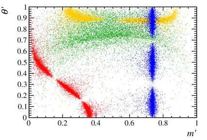
Since, particularly in $B$ decays, signal events tend to populate regions close to the kinematic boundaries of the DP, it can be convenient to use a co-ordinate transformation into the so-called square Dalitz plot (SDP) [33]. The SDP is defined by variables $m^{\prime}$ and $\theta^{\prime}$ that have validity ranges between 0 and 1 and are given by

$$m^{\prime}\equiv\frac{1}{\pi}\cos^{-1}\left(2\frac{m_{12}-m^{\rm min}_{12}}{m^{\rm max}_{12}-m^{\rm min}_{12}}-1\right)\hskip 28.45274pt{\rm and}\hskip 28.45274pt\theta^{\prime}\equiv\frac{1}{\pi}\theta_{12}\,,$$ (27)

where $m^{\rm max}_{12}=m_{P}-m_{d_{3}}$ and $m^{\rm min}_{12}=m_{d_{1}}+m_{d_{2}}$ are the kinematic limits of $m_{12}$ allowed in the $P\rightarrow d_{1}d_{2}d_{3}$ decay, while $\theta_{12}$ is the helicity angle between $d_{1}$ and $d_{3}$ in the $d_{1}d_{2}$ rest frame, as explained in Sec. 2.4. Similar to how a choice of DP variables must be made, the SDP can be defined in several different ways. The expressions of Eq. (27) correspond to the choice used in Laura⁺⁺, which must be employed consistently whenever a SDP is used.

To transform between DP and SDP representations, it is necessary to ensure correct normalisation. This is achieved by including the determinant of the Jacobian of the transformation, which is given by

$$\left|J\right|=4\,p\,q\,m_{12}\frac{\partial m_{12}}{\partial m^{\prime}}\frac{\partial\cos\theta_{12}}{\partial\theta^{\prime}}\,,$$ (28)

where $p$ and $q$ are evaluated in the $d_{1}d_{2}$ rest frame and the partial derivatives evaluate to

$$\frac{\partial m_{12}}{\partial m^{\prime}} = -\frac{\pi}{2}\sin(\pi m^{\prime})\left(m^{\rm max}_{12}-m^{\rm min}_{12}\right)\,,$$

$$\frac{\partial\cos\theta_{12}}{\partial\theta^{\prime}} = -\pi\sin(\pi\theta^{\prime})\,.$$ (29)

The SDP coordinate system has several advantages that apply whenever there is a need to bin the phase space, which are illustrated in Fig. 3. Firstly, the regions near the kinematic boundary are spread out, which means that these regions where the signal is often concentrated and where also there can be rapid variation in efficiency and background distributions can be treated with a much finer resolution, even while maintaining a uniform binning. Secondly, the kinematic boundary is perfectly aligned with the bin edges.

Figure 3: Illustration of the transformation between conventional and square Dalitz plot representations, for resonances in the ${{B}^{0}_{s}}\rightarrow{{\kern 1.99997pt\overline{\kern-1.99997ptD}{}}{}^{0}}{{\pi}^{+}}{{K}^{-}}$ decay (here the final-state particles are ordered following the $d_{1}d_{2}d_{3}$ convention of Laura⁺⁺). Compared to the same DP shown in Fig. 1, a fake ${{\kern 1.99997pt\overline{\kern-1.99997ptD}{}}{}^{0}}{{\pi}^{+}}$ resonance, with parameters corresponding to those of the ${D}^{*}_{2}(2460)^{+}$ state (blue points) has been added in order to better visualise the transformation in relevant DP regions.

4.2 Isobar dynamics and resonances

Once the kinematics of a particular decay mode have been established, the structure of the signal DP model can be by defined by creating a LauIsobarDynamics object. Components of the model are specified using the addResonance member function, which requires:

• the name of the resonance,

• an integer that specifies which of the daughters is the bachelor particle, and hence in which invariant mass spectrum this resonance will appear (1 for $m_{23}$, 2 for $m_{13}$, 3 for $m_{12}$ or 0 for some nonresonant models),

• an enumeration to select the form of the dynamical amplitude.

Appendix C contains lists of the names of the allowed resonances along with their nominal mass, width, spin, charge and Blatt–Weisskopf barrier radius. This information is all automatically retrieved from LauResonanceInfo records that are stored in the LauResonanceMaker class. Appendix C also provides information on how to account for a state that is not already included in Laura⁺⁺, and how to change the nominal values of the properties of any resonance. Appendix A gives details of all the dynamical amplitude forms that are currently implemented in the package and in Table A1 supplies the corresponding enumeration types. Examples of usage are given in Sec. 7.1.

The signal model may also include contributions that do not interfere with the other resonances in the DP. These may arise due to decays that proceed via intermediate long-lived, i.e. negligible natural width, states; an example is the contribution from ${{{B}^{-}}}\rightarrow{{D}^{0}}{{\pi}^{-}}$, ${{D}^{0}}\rightarrow{{K}^{-}}{{\pi}^{+}}$ in ${{{B}^{-}}}\rightarrow{{K}^{-}}{{\pi}^{+}}{{\pi}^{-}}$ decays. Experimentally, such components can be considered either as signal or background, and selection requirements (e.g., based on the consistency of the three daughter tracks originating from the same vertex position) may be used to suppress them, but in certain cases some contribution will remain. Within Laura⁺⁺, the user can choose how to treat such contributions. When considered as part of the signal model, non-interfering components can be added with the addIncoherentResonance member function, which has the same number and type of arguments as the addResonance function. In this case the form of the dynamical amplitude should be specified as GaussIncoh, and the width should be changed to correspond to the experimental resolution. Note that the resolution for incoherent contributions is handled in a different way to the approach described in Sec. 3 and Sec. 5.2. As part of the signal model, a non-interfering component will contribute to the denominator of the fit fractions, but it is simple for the user to subtract it from the results since there is no interference with other components.

When building the model, Laura⁺⁺ performs a simple check of charge conservation, while angular momentum is conserved by construction. However, the onus is on the user to make sure that the strong decays of resonances included in the model respect conservation of parity and flavour quantum numbers, since these are not checked by the code. In order to help with this, a summary of all resonances used in the model is printed out during the initialisation.

The complex dynamical amplitudes $R(m)$ of the various resonance forms are defined using classes that inherit from the abstract base class LauAbsResonance. For example, the relativistic Breit–Wigner lineshape is defined within the LauRelBreitWignerRes class. All such classes implement the resAmp member function that returns a LauComplex class that represents the amplitude at the given value of the relevant two-body invariant mass. The LauAbsResonance base class implements the calculation of the angular distribution factor. Those amplitude forms that require the calculation of the Blatt–Weisskopf factors make use of the LauBlattWeisskopfFactor helper class.

4.3 Symmetry

If the decay of $P$ contains two identical daughters, such as in ${{{B}^{+}}}\rightarrow{{\pi}^{+}}{{\pi}^{+}}{{\pi}^{-}}$, then the DP will be symmetric. As mentioned in Sec. 2.4, the identical particles should be positioned as $d_{1}$ and $d_{2}$. This situation is automatically detected by LauDaughters and the information propagated to the amplitude model. In this case, it is required only to define the resonances for the pair $d_{1}d_{3}$; the amplitude is automatically symmetrised by LauIsobarDynamics by flipping the invariant-mass squared variables $m^{2}_{13}\leftrightarrow m^{2}_{23}$, recalculating the amplitude and summing.

When all of the daughters are identical, for example in ${{B}^{0}}\rightarrow{{K}^{0}_{\rm\scriptscriptstyle S}}{{K}^{0}_{\rm\scriptscriptstyle S}}{{K}^{0}_{\rm\scriptscriptstyle S}}$, it is again only needed to define the resonances for one of the pairs (usually $d_{1}d_{3}$). For this fully symmetric case, LauIsobarDynamics automatically performs the necessary symmetrisation of the amplitude by cyclically rotating the invariant-mass squared variables ($m^{2}_{12}\rightarrow m^{2}_{23}$, $m^{2}_{23}\rightarrow m^{2}_{13}$, $m^{2}_{13}\rightarrow m^{2}_{12}$) and flipping them ($m^{2}_{13}\leftrightarrow m^{2}_{23}$).

4.4 Normalisation of signal model

Various integrals of the dynamical amplitude across the DP need to be calculated in order to normalise the signal PDF given by Eq. (21), as well as for calculating the fit fractions for individual resonances defined in Eqs. (22) and (23). Since the $c_{j}$ coefficients are constant across the DP, only the amplitude terms $F_{j}$ need to be integrated. In general, these integrals cannot be found analytically, so Gauss–Legendre quadrature is used to evaluate them numerically. This is achieved by dividing the DP into an unequally spaced grid whose points correspond to the abscissa co-ordinates from the quadrature procedure. The granularity of the grid is chosen to ensure sufficiently precise integration, as discussed in more detail below. The $F_{j}$ terms are then multiplied by the quadrature weights and summed over all grid points that lie within the DP boundary. To remove the quadratic variable dependence, and to improve numerical precision, the DP area element $dm^{2}_{13}\,dm^{2}_{23}$ is replaced by $dm_{13}\,dm_{23}$ multiplied with the Jacobian factor $4\,m_{13}\,m_{23}$. This means that the normalisation of the total amplitude $\cal{A}$ is given by

$${\int\!\!\int_{\rm DP}~{}{|{\cal A}|^{2}}~{}dm^{2}_{13}\,dm^{2}_{23}}\approx\sum_{a=1}^{N_{a}}\sum_{b=1}^{N_{b}}{4h_{a}h_{b}w_{a}w_{b}|{\cal{A}}|^{2}}\,,$$ (30)

where $w_{a}$ ($w_{b}$) are the weights for the Gauss–Legendre quadrature abscissa values $h_{a}$ ($h_{b}$), which correspond to the grid points along the $m_{13}$ ($m_{23}$) axis, and the amplitude $\cal{A}$ is evaluated for all abscissas inside the DP kinematic boundary. An equivalent expression is used for normalisation of the experimental signal PDF of Eq. (24). The number of points $N_{a}$ ($N_{b}$) is set by dividing the $m_{13}$ ($m_{23}$) mass range by a default “bin width” $\delta m$ of 5${\mathrm{\,Me\kern-1.00006ptV\!/}c^{2}}$, which can be changed using the setIntegralBinWidths function in LauIsobarDynamics, giving $\sim 1000$ integration bins along each mass axis for $B$ decays. It is important to realise that $\delta m$ is not, in general, equal to the separation between neighbouring abscissa points. The LauIntegrals class handles the calculation of the general weights and abscissas for the integration range $(-1,1)$, while the LauDPPartialIntegralInfo class scales these using the half-ranges and mean values of $m_{13}$ and $m_{23}$, following the numerical recipe given in Ref. [63]. This information is then used within the LauIsobarDynamics class to find the normalisation integral for the total amplitude, as well as the integrals for the fit fractions.

If the DP contains narrow resonances with widths below a threshold value, which defaults to 20${\mathrm{\,Me\kern-1.00006ptV\!/}c^{2}}$ but can be changed using the setNarrowResonanceThreshold function in LauIsobarDynamics, then the quadrature grid is split up into smaller regions to ensure that the narrow lineshapes are integrated correctly. The range, in the invariant mass of the resonance daughters, for these sub-regions is taken to be $m_{0}\pm 5\Gamma_{0}$, where $m_{0}$ and $\Gamma_{0}$ are the nominal mass and width of the resonance. The number of quadrature points ($\sim 1000$) along each sub-grid axis is set by dividing the resonance mass range (ensuring the limits stay within the DP boundary) by a $\delta m$ value which defaults to 1% of $\Gamma_{0}$ and is configurable using the setIntegralBinningFactor function in LauIsobarDynamics. Grid regions that are outside the narrow resonance bands use the default bin width. When there are narrow resonances along the diagonal axis $m_{12}$, the integration scheme switches to use the SDP defined in Section 4.1.1. The number of points on the integration grid defaults to 1000 for each of the $m^{\prime}$ and $\theta^{\prime}$ axes. This can be tuned using the setIntegralBinWidths function.

The fact that resonance parameters can float in the fit means that the integrals will need to be recalculated if and when those values change. In order to minimise the amount of information that needs to be recalculated at each fit iteration, a caching and bookkeeping system is employed that stores the amplitudes of each component of the signal model as well as the Gauss–Legendre weights and the efficiency for every point on the integration grid. At each fit iteration it then checks which, if any, resonance parameter values have changed and with which amplitudes those parameters are associated. Only those affected amplitudes are recalculated (for each integration grid point and for each event in the data sample). While greatly improving the speed of fits, this comes at some cost in terms of memory usage, in particular if the integration grid is very fine. If the number of grid points is extremely large a warning message is printed, which recommends that the integration scheme be tuned using the setNarrowResonanceThreshold and setIntegralBinningFactor functions of LauIsobarDynamics to reduce the number of points.

4.5 Signal model and amplitude coefficients

Having defined the signal PDF for $P\rightarrow d_{1}d_{2}d_{3}$, as in Eq. (24), it is necessary to define the parameterisation of the complex coefficients $c_{j}$ defined in Eq. (3). Several different parametrisations have been used in the literature and are available in Laura⁺⁺— a complete list is given in Table 1. These can be separated into two categories: cases in which it is assumed that there is no difference between the decay of $P$ and its $C\!P$-conjugate ${\kern 1.79993pt\overline{\kern-1.79993ptP}{}}$ and cases in which such $C\!P$-violating differences are accommodated.

In the former case, the signal model is constructed by passing the corresponding LauIsobarDynamics instance to a LauSimpleFitModel object, which inherits from the abstract base class LauAbsFitModel. The fit model classes implement the functions needed to generate events according to the DP model as well as to perform fits to data. In the latter case, the decays of each of $P$ and ${\kern 1.79993pt\overline{\kern-1.79993ptP}{}}$ should be represented by their own LauDaughters instance. These are used to construct two instances of LauIsobarDynamics, which in turn are used to construct an instance of the LauCPFitModel class that, like LauSimpleFitModel, also inherits from LauAbsFitModel.

The $F_{j}$ terms in Eq. (21) are calculated using the amplitudes that make up the LauIsobarDynamics model. The complex coefficients $c_{j}$ are each represented by an object inheriting from the LauAbsCoeffSet base class, which provides an abstract interface for combining a set of real parameters to form the complex $c_{j}$. Each coefficient is constructed by providing the name of the resonance $j$ and a series of parameter values that will be used to form the complex number $c_{j}$. They are then applied to the model using the setAmpCoeffSet function of the LauSimpleFitModel or LauCPFitModel class. Checks are made to ensure that the coefficient name matches that of one of the components of the isobar model. The coefficient is then assigned to that component. As such the various coefficients are reordered to match the ordering in the LauIsobarDynamics model(s).

Table 1: List of coefficient sets to represent $c_{j}$ in Eq. (3), separated into cases where $C\!P$ conservation is assumed and those where $C\!P$ violation is accommodated in the model. Where parameters are preceded by $\pm$ signs in the expressions for $c_{j}$, the $+$ ($-$) sign corresponds to the usage for $P$ (${\kern 1.79993pt\overline{\kern-1.79993ptP}{}}$) decays. The corresponding class for each set is LauLabelCoeffSet, where Label is the set label given below.

Set label	Parameters	$c_{j}$
MagPhase	$r$, $\phi$	$re^{i\phi}$
RealImag	$x$, $y$	$x+iy$
BelleCP	$a$, $b$, $\delta$, $\phi$	$ae^{i\delta}(1\pm be^{i\phi})$
CartesianCP	$x$, $y$, $\delta_{x}$, $\delta_{y}$	$x\pm\delta_{x}+i(y\pm\delta_{y})$
CartesianGammaCP	$x$, $y$, $x_{{C\!P}}$, $y_{{C\!P}}$, $\Delta x_{{C\!P}}$, $\Delta y_{{C\!P}}$	$(x+iy)[1+x_{{C\!P}}\pm\Delta x_{{C\!P}}+$
		$i(y_{{C\!P}}\pm\Delta y_{{C\!P}})]$
CleoCP	$a$, $b$, $\delta$, $\phi$	$(a\pm b)e^{i(\delta\pm\phi)}$
MagPhaseCP	$r$, $\phi$, $\bar{r}$, $\bar{\phi}$	$re^{i\phi}$ for $P$
		$\bar{r}e^{i\bar{\phi}}$ for ${\kern 1.79993pt\overline{\kern-1.79993ptP}{}}$
PolarGammaCP	$x$, $y$, $r$, $\delta$, $\gamma$	$(x+iy)(1+re^{i(\delta\pm\gamma)})$
RealImagCP	$x$, $y$, $\bar{x}$, $\bar{y}$	$x+iy$ for $P$
		$\bar{x}+i\bar{y}$ for ${\kern 1.79993pt\overline{\kern-1.79993ptP}{}}$
RealImagGammaCP	$x$, $y$, $x_{{C\!P}}$, $y_{{C\!P}}$, $\bar{x}_{{C\!P}}$, $\bar{y}_{{C\!P}}$	$(x+iy)(1+x_{{C\!P}}+iy_{{C\!P}})$ for $P$
		$(x+iy)(1+\bar{x}_{{C\!P}}+i\bar{y}_{{C\!P}})$ for ${\kern 1.79993pt\overline{\kern-1.79993ptP}{}}$

5 Implementation of efficiency and resolution effects

As discussed in Sec. 3, in an experimental analysis it is usually necessary to modify the signal PDF in order to account for effects such as the variation of the reconstruction and selection efficiency over the DP and detector resolution or misreconstruction. In this section we describe the classes and methods in the Laura⁺⁺ package that are used to implement these modifications to the pure physics PDF described previously.

All experimental effects are handled within Laura⁺⁺ through histograms. Optional spline interpolation is available to smooth effects due to the finite size of samples used to obtain the histograms. In some analyses it may be possible to obtain reliable parametric descriptions of, for example, the efficiency variation over the DP. Where this is a possible and desirable approach the user can simply generate a histogram from the parametric shape and use that as input. The granularity of the histogram can be as fine as necessary to describe local variations; often the limiting factor on the binning will be the size of the sample used to obtain the shape.

5.1 Efficiency

The variation of the signal efficiency over the DP, $\epsilon(m^{2}_{13},m^{2}_{23})$, is implemented by the LauEffModel class. Its constructor requires a LauDaughters object, which defines the kinematic boundary, as well as a LauVetoes object, which is used to specify any region in the DP that has been excluded from the analysis (perhaps to remove particular sources of background or to exclude a region of phase space where the efficiency variation is poorly understood). The signal efficiency is set to zero inside a vetoed region; the resulting discontinuity at the boundary motivates different treatment of vetoes to other sources of inefficiency that vary smoothly across the DP. Vetoes can be added using the addMassVeto or addMassSqVeto functions of the LauVetoes class, which require the bachelor daughter index as well as the lower and upper invariant mass (or mass-squared) values for each exclusion region. Since version v3r2 of Laura⁺⁺, vetoes are automatically symmetrised as appropriate for DPs containing two or three identical particles in the final state.

All other information on the efficiency variation over the DP needs to be supplied in the form of a uniformly binned two-dimensional Root histogram. Alternatively, a set of histograms can be provided; in this case the total efficiency is obtained by multiplying the efficiencies at the appropriate position in phase space from each of the components. This provides a convenient way to assess the impact of systematic uncertainties from different contributions to the total efficiency. Each of these component efficiency histograms can have different binning.

Efficiency histograms will usually be constructed by applying all selection requirements to a simulated sample of signal decays that has been passed through a full detector simulation. A ratio is then formed of all decays that survive the reconstruction and selection to all those that were originally generated. Since the effect of explicit vetoes in the phase space is separately accounted for, it is advised that these are not applied when constructing the numerator of the efficiency histogram.

As previously mentioned in Sec. 4.1.1, signal events often occupy regions close to the kinematic boundaries. The SDP transformation defined in Eq. (27) can be used to spread out these regions so that the efficiency variation can be modelled more accurately. As such, the LauEffModel class will accept histograms that have been created in either $m^{2}_{13}$–$m^{2}_{23}$ or $m^{\prime}$–$\theta^{\prime}$ space.

The histogram can then be supplied to the LauEffModel class via the setEffHisto or setEffSpline function as appropriate. Where the total efficiency is to be obtained from the product of several components, further histograms can be included with the addEffHisto and addEffSpline functions. In each case, a boolean argument squareDP is used to indicate the space in which the histogram has been defined. For symmetric DPs, there is also the option to specify that the histogram provided has already been folded and hence only occupies the upper half of the full DP (or the corresponding lower half of the SDP). Internally, each histogram is stored as a Lau2DHistDP or Lau2DSplineDP object, which implement (optional) bilinear or cubic spline interpolation methods, respectively.

Functionality is also available to help estimate systematic uncertainties due to imperfect knowledge of the efficiency variation by creating Gaussian fluctuations in the bin entries. The fluctuations are based on the uncertainties provided by the user, which, depending on the function used to provide the histogram, can be asymmetric. It is up to the user as to whether the provided uncertainties are simply due to the limited size of the simulated sample or whether they also account for effects such as possible disagreements between data and simulation. The fluctuations are activated by providing optional boolean arguments to the function where the histogram is provided.

5.2 Resolution

The self cross-feed component of the signal likelihood, modelled as described in Eq. (25), is implemented using information from the LauScfMap class, which stores all possible values of $w_{\rm scf}$ via its setHistos function. As for the description of the efficiency, the histograms used to describe $w_{\rm scf}$ and $f_{\rm scf}$ can be constructed in either $m^{2}_{13}$–$m^{2}_{23}$ or $m^{\prime}$–$\theta^{\prime}$ space. However, to simplify the implementation in Laura⁺⁺ it is currently required that all histograms related to the description of resolution have the same binning.

The implementation proceeds as follows. Consider a SDP describing the true position, $s_{\rm true}$, divided into a uniformly binned two-dimensional histogram. Each bin will have associated with it another two-dimensional histogram, with identical binning, whose entries give the migration probability $w_{\rm scf}(s_{\rm reco},s_{\rm true})$ of the true position (given by the original bin centre) being reconstructed in the bin that contains $s_{\rm reco}$. These can be constructed as follows:

• Each histogram contains only the events that were generated in a given true bin.

• The events are plotted at their reconstructed co-ordinates.

• The histogram is then normalised.

Some histograms may be empty if there were no events generated in that bin, although this is of course dependent on the size of the samples used and the size of the bins. The order of the histograms in the vector supplied to the setHistos function should be in terms of the Root “global bin number”.

The splitSignalComponent method of LauSimpleFitModel and LauCPFitModel takes a LauScfMap object as an argument, as well as a two-dimensional Root histogram whose entries give $f_{\rm{scf}}(s_{\rm{true}})$. The fit models then use this information to evaluate the self cross-feed contribution to the likelihood. In the ideal case of Eq. (25) this is described by an integral; in practice this becomes a summation,

$$\begin{array}[]{c}\int f_{\rm scf}(s_{\rm true})\,w_{\rm scf}(s_{\rm reco},s_{\rm true})\,{\cal P}_{\rm sig}(s_{\rm true})\,ds_{\rm true}\\ \hookrightarrow\\ \sum_{i}\left[\left<\hat{f}_{\rm scf}(\hat{s}_{\rm true\,i})\right>\,\left<\hat{w}_{\rm scf}(\hat{s}_{\rm reco},\hat{s}_{\rm true\,i})\right>\,{\cal P}_{\rm sig}(\hat{s}_{\rm true\,i})\,\frac{\Delta\Omega(\hat{s}_{\rm true\,i})}{\Delta\Omega(\hat{s}_{\rm reco})}\right]\,,\end{array}$$ (31)

where the hat ($\,\hat{}\,$) notation is used to indicate quantities evaluated in the SDP (as is the case in this example), and the bracket ($\,\left<\,\right>\,$) notes quantities obtained from histograms. The pure signal PDF ${\cal P}_{\rm sig}$ is as in Eq. (24), evaluated at the position corresponding to the SDP point at the centre of the $\hat{s}_{\rm true\,i}$ bin. The phase space factors $\Delta\Omega$ are equal to $\Delta m^{\prime}\Delta\theta^{\prime}\left|J\right|$ where the SDP bin size is given by $\Delta m^{\prime}\Delta\theta^{\prime}$ and the Jacobian of the SDP transformation is that of Eq. (28); since equal binning is required, the ratio of phase space factors reduces to a ratio of Jacobians.

6 Implementation of background components

6.1 Dalitz-plot distributions

Backgrounds in the data sample can be taken into account by including them in the total likelihood defined in Eq. (26). This means that the DP distributions of all background categories need to be provided. In an analogous way to the implementation of the signal efficiency described in the previous section, the DP distribution of each background category is represented with a uniformly binned two-dimensional Root histogram.

Background contributions are handled in Laura⁺⁺ as follows. Firstly, the names of all background categories need to be provided to the fit model via the setBkgndClassNames function of the appropriate LauAbsFitModel class. Then, each named category needs to have its DP distribution defined and added to the fit model. This is achieved by supplying one (or more if the model subdivides the data to account for effects such as $C\!P$ violation) LauBkgndDPModel object. The constructor of the LauBkgndDPModel class requires pointers to the usual LauDaughters and LauVetoes objects. The histogram is supplied to the LauBkgndDPModel object via its setBkgndHisto (setBkgndSpline) function, and is then internally stored as a Lau2DHistDPPdf (Lau2DSplineDPPdf) object that implements bilinear (cubic spline) interpolation. The PDF value is then calculated as the interpolated number of background events $B(m^{2}_{13},m^{2}_{23})$ divided by the total integrated area of the histogram:

$${\cal P}_{\rm{bkgnd}}=\frac{B(m^{2}_{13},m^{2}_{23})}{\int\!\!\int_{\rm DP}~{}B(m^{2}_{13},m^{2}_{23})~{}dm^{2}_{13}\,dm^{2}_{23}}\,.$$ (32)

Like signal events, backgrounds also tend to populate regions close to the kinematic boundaries of the DP. Therefore, the use of histograms in the SDP space can improve the modelling of backgrounds. This is achieved by providing a histogram in $m^{\prime}$–$\theta^{\prime}$ space and setting the squareDP boolean flag to true in the setBkgndHisto or setBkgndSpline functions of LauBkgndDPModel. The normalisation of these PDFs then automatically includes the Jacobian for transforming from normal to square Dalitz-plot space.

Some special treatment is necessary for backgrounds modelled from sources that contain contributions that are vetoed in the DP fit. Following the example of Sec. 3, the combinatorial background to ${{{B}^{-}}}\rightarrow{{K}^{-}}{{\pi}^{+}}{{\pi}^{-}}$ decays may be modelled from a sideband in the $B$ candidate mass distribution that also contains some genuine ${{D}^{0}}\rightarrow{{K}^{-}}{{\pi}^{+}}$ decays. The histogram binning will introduce some smearing of such contributions, so that once the veto is applied later some residual background may remain. In principle this can be avoided with sufficiently fine histogram bins, but this will often be impractical due to finite sample sizes. Instead, and in contrast to the procedure for efficiency histograms described in Sec. 5.1, the veto should be applied when the background histogram is made. This will, however, lead to an underestimation of the background that is being modelled (in the example above, of the random combinations of three tracks) within bins that lie partially inside the vetoed regions. To correct for this effect, each background histogram needs to be divided by another histogram (with the same binning) whose entries contain the fraction of events, generated from a high statistics sample that is uniform in phase space, that lie outside any veto region; bins that are completely outside (inside) a veto have a weight of unity (zero), and division by zero is interpreted as zero weight. The histogram supplied to LauBkgndDPModel should already have had this correction applied to it.

6.2 Other discriminating variables

When fitting a data sample that contains (significant) backgrounds, additional discriminating variables can be included in the total likelihood function defined in Eq. (26), in order to provide improved separation between signal and background categories. Examples of such discriminating variables include the mass of the parent particle $P$ candidate and the output of a multivariate discriminant to separate signal from background. Assuming that all of the variables $\vec{x}=(x_{1},x_{2},...,x_{n})$ are uncorrelated, the PDF ${\cal P}^{j}_{k}$ of the signal or background category $k$, for event $j$, is given by the product of the individual variable PDFs (including that of the DP distribution): ${\cal P}^{j}_{k}(\vec{x})={\cal P}^{j}_{k}(x_{1})\times{\cal P}^{j}_{k}(x_{2})\times...\times{\cal P}^{j}_{k}(x_{n})$.

Additional PDFs are represented by classes that inherit from LauAbsPdf, whose constructor requires the variable name, a vector of the PDF parameters, as well as minimum and maximum abscissas that specify the variable range. Each class implements the member function for evaluating the PDF function at a given abscissa value and that for evaluating the maximum value of the PDF in the fitted range. A list of classes that can be used for additional PDFs is given in App. D. Each PDF needs to be added to the fit model; for LauSimpleFitModel (LauCPFitModel), signal PDFs are added using the setSignalPdf (setSignalPdfs) function, self cross-feed PDFs are included via setSCFPdf (setSCFPdfs) function, and background PDFs are added with the setBkgndPdf (setBkgndPdfs) function.

An alternative approach is to perform first a fit to some or all of the other discriminating variables to determine the yields of signal and background. These values can then be fixed in the fit to the DP to extract the amplitude parameters. Requirements can also be imposed on those variables, before or after such a fit, in order to enhance the signal purity among the events entering the DP fit. This approach will have slightly reduced sensitivity but avoids the need to model correlations between the DP and the other variables (although classes are provided that allow the modelling of such correlations, see App. D.13). It is possible to fit only other discriminating variables, i.e. excluding the DP variables, in Laura⁺⁺ through the useDP function of LauAbsFitModel, which takes a boolean argument.

7 Work flows

The Laura⁺⁺ package is designed to perform three main work flows:

• Monte Carlo generation of toy datasets from a defined PDF,

• fitting a defined PDF to an input data set,

• calculating per-event weights for an input data sample (usually full detector simulation) from a defined DP model.

In this section we describe the setup stages that are common to all tasks, then each of the three work flows in turn, and finally some variations that are available. Code taken from the various examples included with the package is used to illustrate many of these points. These code snippets are in C++ but it is also possible to use the python bindings that are generated by rootcling when the Laura⁺⁺ library is compiled and to write the application code in python. An example that demonstrates how to do this, GenFit3pi.py, is included in the package since version v3r3.

7.1 Common setup

The first setup task is to define the DP with which we are working. As mentioned in Section 4.1 this is achieved through the declaration of a LauDaughters object:

⬇

bool squareDP = true;

LauDaughters* daughters = new LauDaughters("B+", "pi+", "pi+", "pi-", squareDP);

specifying the types of the parent particle and the three daughters. The final argument specifies whether or not we will be using the variables of the SDP (defined in Section 5) and as such whether these should be calculated — if they are not required then it is more efficient to switch off this calculation.

Next to be defined is the efficiency model, including any explicit vetoes in the Dalitz plane:

⬇

LauVetoes* vetoes = new LauVetoes();

LauEffModel* effModel = new LauEffModel(daughters, vetoes);

Without further specification, this will give a uniform efficiency (of unity) over the DP. This can be modified by specifying vetoes and/or supplying the efficiency variation in the form of a histogram, e.g.

⬇

vetoes->addMassVeto(2, 1.7, 1.9); // D0 veto, covering 1.7 < m13 < 1.9 GeV/c^2

TH2* effHist = ...;

effModel->setEffHisto(effHist);

The next step is to define the signal amplitude model. Before defining any resonances the first thing to be done is to specify the Blatt–Weisskopf barrier radii to be used for the different resonances. This is done by accessing the singleton LauResonanceMaker factory object:

⬇

LauResonanceMaker& resMaker = LauResonanceMaker::get();

resMaker.setDefaultBWRadius( LauBlattWeisskopfFactor::Parent, 5.0 );

resMaker.setDefaultBWRadius( LauBlattWeisskopfFactor::Light, 4.0 );

It is possible also to specify whether any of these values should be floated in the fit. By default they are fixed to the specified value. The isobar model can now be created and the various resonances added to it:

⬇

LauIsobarDynamics* sigModel = new LauIsobarDynamics(daughters, effModel);

LauAbsResonance* reson(0);

reson = sigModel->addResonance("rho0(770)", 1, LauAbsResonance::GS);

reson = sigModel->addResonance("f_0(980)", 1, LauAbsResonance::Flatte);

reson->setResonanceParameter("g1",0.2);

reson->setResonanceParameter("g2",1.0);

reson = sigModel->addResonance("f_2(1270)", 1, LauAbsResonance::RelBW);

reson = sigModel->addResonance("rho0(1450)", 1, LauAbsResonance::RelBW);

reson = sigModel->addResonance("NonReson", 0, LauAbsResonance::FlatNR);

Note how the returned pointer to the added resonance can be used to modify parameters of the resonance. It is also possible to specify that resonance parameters should be floated in the fit using the LauAbsResonance::floatResonanceParameter member function.

The fit model can now be created based on the isobar model that has just been defined.

⬇

LauSimpleFitModel* fitModel = new LauSimpleFitModel(sigModel);

And the complex coefficients for each resonance defined using one of the various parametrisations defined in Table 1, in this case using a simple magnitude and phase form:

⬇

std::vector<LauAbsCoeffSet*> coeffset;

coeffset.push_back( new LauMagPhaseCoeffSet("rho0(770)", 1.00, 0.00, true, true) );

coeffset.push_back( new LauMagPhaseCoeffSet("f_0(980)", 0.27, -1.59, false, false) );

coeffset.push_back( new LauMagPhaseCoeffSet("f_2(1270)", 0.53, 1.39, false, false) );

coeffset.push_back( new LauMagPhaseCoeffSet("rho0(1450)", 0.37, 1.99, false, false) );

coeffset.push_back( new LauMagPhaseCoeffSet("NonReson", 0.54, -0.84, false, false) );

for (std::vector<LauAbsCoeffSet*>::iterator iter=coeffset.begin(); iter!=coeffset.end(); ++iter) {

fitModel->setAmpCoeffSet(*iter);

}

The boolean arguments to the constructor indicate whether the value should be fixed in the fit. Since Laura⁺⁺ version v3r1, the ordering of the components is defined by the isobar model (first all coherent resonances in order of addition to the isobar model, then all incoherent resonances in order of addition), and the coefficients are automatically rearranged to match that order. Thus, the user does not need to worry about the order of the components given here.

To either generate toy datasets or to fit data, it is necessary to specify the number of events in each of the signal and (if appropriate) background categories. The Laura⁺⁺ work flow requires that these values are specified also in the case of weighting data, although they are not used. In the case of fitting data the given values may be floated, as is often appropriate when additional discriminating variables are included in the fit (see Sec. 6.2), or fixed, as is usually necessary when only the DP is being fitted. In the former case, if the doEMLFit option is specified the fitted values of the yields can be expected to have the correct Poisson uncertainties. The user should ensure that the specified number of events in the signal and background categories correspond to the number of events in the data file that will be read in to that fit. The number of signal events is set as follows:

⬇

LauParameter * nSigEvents = new LauParameter("nSigEvents",500.0,-1000.0,1000.0,false);

fitModel->setNSigEvents(nSigEvents);

The number of experiments, as well as which experiment to start with, must also be specified:

⬇

const int nExpt(1);

const int firstExpt(0);

fitModel->setNExpts( nExpt, firstExpt );

The above example values are appropriate when fitting a single data sample. If generating and/or fitting toy pseudoexperiments then a larger number of experiments can be specified. Optionally, models for one or more background categories can also be specified along with the corresponding event yields.

Finally there are various control and configuration options that can be set, which are listed in Table 2. Once all the configuration is completed, the required operation (toy generation, fitting, or event weighting) can be run:

⬇

fitModel->run( command, dataFile, treeName, rootFileName, tableFileName );

where all the arguments are strings, with the following purposes

• command is either “gen”, “fit” or “weight”;

• dataFile and treeName specify the name of the Root file and tree from which the data should be read or to which the generated data should be written (depending on the mode of operation);

• rootFileName specifies the name of the Root file to which the results of the fit (fit convergence status, likelihood, parameter values, uncertainties, correlations, etc.) should be saved;

• tableFileName specifies the name of the LaTeX file to which the results of the fit or generation should (optionally) be written.

The run function performs the initialisation of all the PDFs that have been defined and checks the internal consistency of the model, e.g. that all event categories have a PDF defined for each variable. All the parameters of the model are gathered into a single list and the bookkeeping of those parameters that affect the DP normalisation is set up. Any constraints on the model parameters, both on individual and on particular specified combinations of parameters, are also recorded. Following these initialisation steps, the particular routines for toy generation, fitting, or weighting of events are called, depending on the specified command. Each of these routines are described in the following sections.

Table 2: Control and configuration options for all fit models.

Function name	Description
useDP	Toggle use of the DP PDF in the likelihood
doSFit	Activate per-event weighting of events in likelihood fit
doEMLFit	Toggle use of the extended maximum likelihood fit
doTwoStageFit	Toggle use of the two-stage fit
useAsymmFitErrors	Toggle determination of asymmetric uncertainties from the fit, e.g. using MINOS routine in Minuit
useRandomInitFitPars	Toggle randomisation of initial values of isobar parameters
addConstraint	Add a Gaussian constraint on a specified combination of fit parameters
doPoissonSmearing	Toggle Poisson smearing of event yields in toy generation
writeLatexTable	Toggle generation of a LaTeX-formatted summary table
writeSPlotData	Activate calculation of event sPlot weights
compareFitData	Activate automatic generation of toy MC datasets based on fit results

7.2 Toy generation

The generation of ensembles of simplified pseudoexperiments, or toys, is of great importance in Laura⁺⁺. Not only is toy generation used to test the performance of a fitter, to test its stability and study potential biases and/or correlations between fitted parameters, it can also be used to determine uncertainties on parameters (see Sec. 7.3.1). Large samples of toy experiments, generated according to the results of a fit, can also be used to display the results of the fit projected onto any variable in any region of the phase space. This is often a convenient way of drawing the result of the fit, including contributions from separate components.

The first action specific to the generation of toy pseudoexperiments is to ensure that the value of each fit parameter is set to that to be used for generation, i.e. the genValue of the LauParameter. Then an ntuple (specifically, a Root TTree) is created in which the generated events will be stored. The branches to be stored are determined based on the PDFs that have been configured in the initialisation step, and will include:

• iExpt and iEvtWithinExpt: these indicate to which pseudoexperiment this event belongs and the position of the event within that experiment;

• evtWeight: a weight for the event that is normally unity but can take other values;

• a set of MC truth branches that indicate whether a given event was generated as signal or one of the background categories, e.g. genSig;

• efficiency: the value of the signal efficiency at the generated DP position (only stored for signal events);

• the DP position in terms of the invariant masses and helicity angle cosines: m12, m13, m23, m12Sq, m13Sq, m23Sq, cosHel12, cosHel13, cosHel23;

• optionally, the position in the SDP coordinates: mPrime and thPrime;

• the values of all other variables used by additional PDFs (see Section 6.2).

Figure 4: Schematic of the LauIsobarDynamics::generate function.

Each experiment is then generated in turn, with the following procedure being followed for each:

1. Determine the number of events to generate for each category. This will either be the value of the yield parameter for the category or, if doPoissonSmearing is specified (see Table 2), will be sampled from a Poisson distribution whose mean is equal to the yield parameter value.

2. For each category, generate the number of requested events. Truth information is stored as to which category the event belongs in branches named “genCAT”, where “CAT” is replaced by the name of the category. For a given event, the variable corresponding to the category being generated will have value 1, while all others will have value 0.

3. For signal events, the generation of the DP position is performed by the LauIsobarDynamics::generate function, the operation of which is shown in Fig. 4. In essence, it is an “accept/reject” method in which the value of the signal model intensity at a given point ($I_{\mathrm{tot}}$ in Fig. 4) is compared with a “ceiling value” ($I_{\mathrm{max}}$ in Fig. 4). Note that the signal model intensity includes effects due to efficiency, vetoes and resolution. Since, in general, it is not computationally efficient to evaluate analytically the maximum value of the intensity, an approximate value is provided by the user via the LauIsobarDynamics::setASqMaxValue function. During the generation process it is checked that a larger value is not encountered. If it is, which would indicate that the generation is biased, the ceiling value is increased and the generation processes starts again from the beginning — all previously generated experiments are discarded. Similarly, too large a ceiling value can make the generation extremely inefficient, so it is also attempted to detect this condition and correct it. If a self cross-feed component has been included in the signal description, once a DP point has been generated it may then be smeared according to the procedure outlined in Section 5.2. Finally, the values of any other discriminating variables can be generated from the corresponding PDFs.

4. For background events, the DP position is generated by the LauBkgndDPModel::generate function. This performs a similar accept/reject routine to that used to generate signal events but here the (optionally interpolated) histogram height is compared with the maximum value of the histogram. There is therefore no need to verify that the encountered value is less than the maximum since this is true by construction. Generated values within a veto region are automatically rejected. Finally, the values of any other discriminating variables are generated from the corresponding PDFs.

Once all experiments have been generated successfully, all events are written to the ntuple.

7.2.1 Embedding events from a file

One possible variation of the scheme just outlined is that events for one or more components of the model are loaded from a Root file rather than being generated from the model PDFs. These events could, for example, be taken from samples of full detector simulation or from data control samples. This procedure can be useful to check for biases that can result due to certain experimental effects not being taken into account in the model (for example, experimental resolution or correlations between fit variables). The events are sampled randomly from the provided file. Depending on the number of events within the samples it may be necessary to sample with replacement, i.e. to allow events to be used more than once.

The exact procedure to enable the embedding of events from a Root file varies slightly depending on the fit model class being used. For LauSimpleFitModel there are two functions embedSignal and embedBkgnd, which can be used to embed signal and background events. For LauCPFitModel there are four functions, to allow separate sources of events in the case that the parent candidate is the particle or antiparticle. The arguments taken by the various functions are, however, essentially the same:

• bkgndClass: in the case of the functions for embedding background events, the name of the background class must be specified as the first argument;

• fileName: the name of the Root file from which the events should be loaded;

• treeName: the name of the TTree object within the file in which the events reside;

• the arguments reuseEventsWithinEnsemble and reuseEventsWithinExperiment control whether or not the sampling of events should allow replacement, firstly within the context of the entire ensemble of experiments being generated (i.e. replacement occurs once each experiment has been generated) and secondly within each experiment (i.e. replacement occurs immediately);

• useReweighting: in the case of embedding signal events, this argument controls whether an accept/reject routine should be used (based on the configured amplitude model) when sampling the events. As discussed in Sec. 7.4, reweighting allows an existing sample to be reused with an alternative model, which can avoid high computational costs associated with obtaining a new sample. This option requires that the both the generated and reconstructed DP coordinates are available in the provided sample since the generated point is used to find the amplitude value to be used in the accept/reject routine but the reconstructed point is the one saved to the output ntuple. This ensures that the effects of experimental resolution and misreconstruction are preserved.

For example, to embed events for the signal component, sampling with immediate replacement, and performing the accept/reject routine:

⬇

fitModel->embedSignal( signalSampleFileName, signalSampleTreeName, kTRUE, kTRUE, kTRUE );

As for other control and configuration functions, such as those in Table 2, these should be called prior to the invocation of the LauAbsFitModel::run function.

7.3 Fitting

While the primary goal of the Laura⁺⁺ package is to facilitate fits to the DP distributions of various decays of interest in data, it is also essential to be able to fit simulated samples such as ensembles of toy experiments generated as discussed above. The same work flow is used for both types of fits. Unbinned maximum likelihood fits are the default in Laura⁺⁺, with extended maximum likelihood fits also an option as noted in Table 2.

The first action specific to the routine for fitting is to create the ntuple in which to store the results of the fit. The branches to be stored are determined based on the PDFs that have been configured in the initialisation step, and will include:

• iExpt: an integer that indicates to which pseudoexperiment the results in this entry in the ntuple belong (zero for a fit to data);

• fitStatus: an integer that indicates whether or not the fit has converged and the degree of accuracy of the resulting covariance matrix (0: fit has failed to converge; 1: fit has converged but covariance matrix is only approximate; 2: the covariance matrix is a full matrix but is forced to be positive definite; 3: the covariance matrix is full and accurate);

• EDM: the estimated distance of the negative log likelihood to the true minimum of the function;

• NLL: the minimised value of the negative log likelihood;

• for each fit parameter: its fitted value, its value at initialisation (for toy data, this will be the true value) and, if it was floated in the fit, its uncertainty (including asymmetric uncertainties, if calculated), pull and global correlation coefficient;

• for each pair of floated fit parameters: their correlation coefficient;

• any extra parameters defined by the fit model, for example, the fit fractions of each component and the interference fit fractions.

If information on the per-event likelihood values is to be stored in order to allow the calculation of sPlot weights [64], this ntuple is also created.

The file containing the data to be fitted is opened and the ntuple retrieved. An error will be returned if the file cannot be opened, if the ntuple cannot be found or if it does not have a flat format, i.e. if it contains stored arrays. Each experiment is then fitted in turn, with the following procedure being followed for each:

1. The data for the given experiment is read into memory. The fit model then passes the data to each of the PDFs such that they can store the values of any variables that they require and also calculate and cache as much information as they can towards (and possibly including) the likelihood value for each event.

2. Optionally (see according to the specification of useRandomInitFitPars; see Table 2), the initial values of the isobar coefficient parameters are randomised.

3. The fitter is initialised by providing it with the list of fit parameters and two boolean options to control whether a two-stage fit (see Sec. 7.3.2) is to be performed and whether asymmetric uncertainties on the fit parameters should be determined.

4. The minimisation of the negative log likelihood is then performed and the uncertainties on the parameters and their correlations are determined. The fit status information and the covariance matrix is stored, and the final values and uncertainties are written back to the fit parameter objects.

5. Some final manipulation of the fit parameter values is performed, e.g. such that phases lie within a particular range, and their pull values are calculated. Quantities derived from the fitted parameters, such as fit fractions, are also calculated. All this information is written to the fit results ntuple.

6. Optionally (see writeSPlotData in Table 2), per-event likelihood information is stored in a separate ntuple.

7. Optionally (see compareFitData in Table 2), and only if the fit was successful, toy MC pseudoexperiments are generated based on the fitted values of the parameters.

Once all experiments have been fitted, information is printed on the success rate of the fits and the fit results ntuple is written to file. Optionally (see writeSPlotData in Table 2), per-event weights are calculated from the likelihood information, using the sPlot method [64], and written to an ntuple.

Due to the often complicated dependence of the likelihood on many parameters in a typical DP analysis, generally there will appear local minima in the likelihood as well as the global minimum. Depending on the starting values of the fit parameters it is possible that the fit will converge to one of the local minima. As such it is highly advisable to perform multiple fits to each data sample using randomised starting values for the parameters of the isobar coefficients. As mentioned in Table 2, the control function useRandomInitFitPars can be used to toggle this behaviour. It is then required only to re-run the executable to obtain a fit based on a new randomised starting point. The applications in the examples directory of the package all include a compulsory command-line option to provide an integer to label the particular fit (or set of fits, if fitting multiple experiments), which is then incorporated into the name of the file containing the ntuple of results for that fit or set of fits. Once all fits have been performed, the fit that returns the best likelihood value can then be selected as the likely global minimum for each experiment. In the examples directory of the package a utility class ResultsExtractor (with accompanying application code) is provided to simplify the process of checking for multiple solutions and extracting the results of the fit that is the candidate global minimum for each experiment. This application writes out a Root file that contains an ntuple that is filled with the candidate global minimum results for each experiment, and a histogram for each experiment that shows the frequency with which each negative log likelihood value is obtained.

7.3.1 Determination of uncertainties

In addition to central values, the fit will return estimates of the uncertainties of each fitted parameter. However, it is typical to want to obtain results not only for the fitted parameters (e.g. complex coefficients for each component of the model) but also for derived parameters (e.g. fit fractions and interference fit fractions). The central values of such derived parameters can be obtained algebraically, however non-linear effects typically render unreliable the determination of uncertainties by standard error propagation. Instead, both central values and uncertainties can be obtained from ensembles of pseudoexperiments generated according to the result of the fit to data. In this approach the uncertainty is obtained from the spread of the distribution of the obtained values in the pseudoexperiments of the parameter of interest. Since this procedure guarantees correct coverage of the uncertainties, and also allows study of effects such as biases and non-linear correlations in the results, it is often preferable to use it also for directly fitted parameters. A further alternative to determining uncertainties on derived parameters is by bootstrapping [65, 66].

7.3.2 Two-stage fit

Fits with large numbers of free parameters can be slow to converge, and may be unstable. These problems can be ameliorated with a two-stage fit, in which certain parameters are initially fixed to specified values while all other parameters are floated. In the second stage, all parameters are floated ensuring that correlations between parameters are correctly accounted for. Note that parameters which are floated only in the second stage cannot have randomised initial values.

One situation in which this fit procedure has been found to be particularly useful is when resonance parameters such as masses and widths are to be floated. Another is when $C\!P$-violation parameters are to be determined. It may be noted that in the CartesianCP coefficient set, one can simultaneously swap $x\leftrightarrow\delta_{x}$, $y\leftrightarrow\delta_{y}$ with an effect that is equivalent to rotating all amplitudes for ${\kern 1.79993pt\overline{\kern-1.79993ptP}{}}$ decays by $\pi$. Such a transformed set of parameters may be hard for the fit to distinguish from the untransformed case. As such a two-stage fit, in which $C\!P$-violation parameters are initially fixed to zero before being floated in the second stage, can help to resolve ambiguities and reject unrealistic multiple solutions.

7.3.3 Relations between fit parameters

There are a number of situations where a given fit parameter can appear in more than one PDF within the likelihood function. Such cases must be flagged in the construction of the fit model in order to ensure that such a parameter is provided only once to the minimiser. Consider the following example that concerns a fit to the invariant mass distribution of candidate ${{{B}^{+}}}\rightarrow{{K}^{+}}{{\pi}^{+}}{{\pi}^{-}}$ decays. The signal is modelled as a Gaussian function, which has two parameters: the mean $\mu$ (corresponding to the mass of the ${{B}^{+}}$) and width $\sigma$ (corresponding to the experimental resolution). A possible background arises from the decay ${{{B}^{+}}}\rightarrow\eta^{\prime}{{K}^{+}};\eta^{\prime}\rightarrow{{\pi}^{+}}{{\pi}^{-}}\gamma$, which is modelled using an ARGUS threshold function (see App. D.1). The threshold parameter of this function is the ${{B}^{+}}$ mass and as such it needs to be encoded in the likelihood function that values of the mean of the signal distribution and the threshold of this background are due to the same parameter. This can be achieved in Laura⁺⁺ using the LauParameter::createClone function, as follows:

⬇

const Double_t mbMin(5.10);

const Double_t mbMax(5.60);

LauParameter* sig_mb_mean = new LauParameter("sig_mb_mean", 5.28, 5.26, 5.30);

LauParameter* sig_mb_sigma = new LauParameter("sig_mb_sigma", 0.20, 0.10, 0.30);

std::vector<LauAbsRValue*> mbPars;

mbPars.push_back(sig_mb_mean);

mbPars.push_back(sig_mb_sigma);

LauAbsPdf* sig_mb_pdf = new LauGaussPdf("mB", mbPars, mbMin, mbMax);

LauParameter* bkg1_mb_m0 = sig_mb_mean->createClone();

LauParameter* bkg1_mb_xi = new LauParameter("bkg1_mb_xi", 20.0, 0.0, 50.0);

mbPars.clear();

mbPars.push_back(bkg1_mb_m0);

mbPars.push_back(bkg1_mb_xi);

LauAbsPdf* bkg1_mb_pdf = new LauArgusPdf("mB", mbPars, mbMin, mbMax);

For the isobar coefficients, it is possible to clone the parameters related to a particular coefficient using the LauAbsCoeffSet::createClone function. One can specify precisely which parameters should be cloned; for example, to allow only $C\!P$-violating parameters to be cloned while the $C\!P$-conserving parameters are still free to vary independently.

Extending the previous example to consider a second possible background from ${{{B}^{+}}}\rightarrow{{K}^{+}}{{\pi}^{-}}{{\pi}^{+}}{{\pi}^{0}}$ decays, where the ${\pi}^{0}$ is not reconstructed, we encounter a case where the threshold parameter is now the difference between the ${{B}^{+}}$ and ${\pi}^{0}$ masses. This scenario can be accommodated in Laura⁺⁺ using a LauFormulaPar object, the constructor of which takes as arguments two strings, which are the name of the compound parameter and the formula to be used to combine the values of the input parameters, and a std::vector of LauParameter objects, which are the input parameters. For the example in question this would be:

⬇

std::vector<LauParameter*> inputPars;

LauParameter* mpiz = new LauParameter("mpiz", LauConstants::mPi0);

inputPars.push_back(sig_mb_mean);

inputPars.push_back(mpiz);

LauFormulaPar* bkg2_mb_m0 = new LauFormulaPar("bkg2_mb_m0", "[0] - [1]", inputPars);

This LauFormulaPar object can be used as one of the parameters for the PDF:

⬇

LauParameter* bkg2_mb_xi = new LauParameter("bkg2_mb_xi", 20.0, 0.0, 50.0);

mbPars.clear();

mbPars.push_back(bkg2_mb_m0);

mbPars.push_back(bkg2_mb_xi);

LauAbsPdf* bkg2_mb_pdf = new LauArgusPdf("mB", mbPars, mbMin, mbMax);

Note the syntax of the formula expression (from the Root TFormula class) where the input parameters are referred to by their index in the std::vector. This syntax allows the usual arithmetic operators to be used as well as functions such as those contained in the TMath namespace.

7.3.4 Blinding of fit parameters

In analyses of data when one is searching for a new signal or searching for $C\!P$ violation it is quite a common practice to “blind” the value of the observables of interest until the event selection and analysis procedures have been finalised [67, 68]. This is commonly achieved by applying an offset, whose value is unknown to the analysts but is determined uniquely from a so-called “blinding string”, when the parameter value is passed to the minimiser or is printed out or otherwise saved at the end of the fit but the true, “unblind”, value is used when calculating the value of the likelihood function. This same technique is used in Laura⁺⁺ in the LauBlind class. The hash of the blinding string is used as the seed for a random number generator, using which a value is sampled from a normal distribution. The offset is then calculated by multiplying this random number by a scaling factor. The blinding string and scaling factor are supplied by the user as follows:

⬇

LauParameter* nSig = new LauParameter("signalEvents", 1000.0, -1000.0, 2000.0, kFALSE);

nSig->blindParameter("dalitzplot",1000.0);

Some care must be taken when defining the scaling factor and the allowed range for the parameter to try and avoid situations where the parameter hits one of the limits. It is also advisable to use different blinding strings for each observable that is to be blinded.

7.3.5 Fitting with external constraints

When the value of a parameter is known from other measurements to within some precision it can be useful to incorporate that information into the likelihood function. This is most commonly achieved by multiplying the likelihood by a Gaussian term, where the mean and width of the Gaussian are the central value and uncertainty from the external source and the abscissa is the value of the parameter in the fit. The addition of such terms to the likelihood expression can be carried out in Laura⁺⁺ using the function LauParameter::addGaussianConstraint, where the arguments are the central value and uncertainty from the external measurement.

In the event that the constraint that needs to be applied is not just on the value of a single parameter but on some combination of fit parameters, this can be achieved via the addConstraint function that is available in all fit model classes. In addition to the mean and width of the Gaussian function, this function takes the following arguments:

• a formula string that specifies how to combine the parameters, which should use the syntax specified by LauFormulaPar (see Sec. 7.3.3);

• a std::vector of strings that are the names of the fit parameters (i.e. the LauParameter objects in the list of fit parameters) whose values are to be used in the formula to calculate the abscissa of the Gaussian function. Note that the order of the names within the vector must match the ordering specified in the formula.

This feature can also be used to perform a scan of the likelihood as a function of any combination of fit parameters. This can be achieved by setting the mean of the Gaussian constraint to one of a range of fixed values, in turn, and setting the width to a sufficiently small value that the quantity is effectively fixed. The negative log-likelihood values obtained from independent fits at each of the scan points can be converted into whatever format is most convenient for the user.

7.3.6 Fitting with background subtraction via sPlot weights

It is possible to perform fits with background subtraction via sPlot weights as proposed in Ref. [69]. In this approach, the weights are obtained from a fit to a discriminating variable in which the signal and any background categories can be distinguished [64]; for the purposes of this discussion this will be considered to be the mass of a $B$ meson candidate for a particular decay to a three-body final state. The advantage of this approach is that it becomes unnecessary to have models for the DP distributions of the background components, and therefore the discussion of Sec. 6 becomes irrelevant. However, the formalism relies on the discriminating variable being uncorrelated with the DP variables. This is likely to be a good approximation for the signal, and also reasonable for combinatorial background. However, additional sources of background such as those involving misidentified decays are likely to have significant correlations between the reconstructed mass and the DP position. Therefore this approach is only valid in the case that such backgrounds are negligible across the whole $B$ candidate mass range — not only the signal region (in this approach to background subtraction, there is no concept of signal region).

Within Laura⁺⁺ this approach to fitting can be implemented by calling the doSFit member function of LauAbsFitModel, which takes as argument the name of the branch that contains the relevant weights, as shown in Table 2. It is also possible to pass an optional second argument, which is a scaling factor that is needed in order to obtain correct uncertainties from the likelihood; this is unnecessary if the uncertainties will be evaluated from pseudoexperiments.

7.3.7 Simultaneous fitting of independent data samples

Simultaneous fits to independent data samples have a variety of applications. For example, the samples may correspond to different experimental conditions and so each may require a different model of the efficiency and background distributions. A simultaneous fit to the various sub-samples allows the statistical power of the full sample to be used to determine the parameters of interest, while accounting as accurately as possible for the changes in the experimental environment. Furthermore, it simplifies the evaluation of systematic uncertainties, in particular the treatment of sources that are correlated among the samples. The technique can also be employed in order to extract information that would otherwise not be feasible, for example to perform a coupled-channel analysis or to exploit flavour symmetries or other relations between decay modes, in order to extract information on $C\!P$ violation observables, as recently carried out in Ref. [70].

The implementation of simultaneous fitting in Laura⁺⁺ is based on the Jfit framework, an overview of which is given here and explained in more detail in Ref. [71]. The framework is based around a master–worker architecture in which the master drives the minimiser, combining the likelihood values for each category that have been calculated by a number of workers. The master and each of the workers run as separate processes that communicate via network sockets. This means that the calculation of the likelihood for each category is performed in parallel, increasing the speed of the computations if sufficient CPU cores are available. Note that the framework even allows the master and various worker processes to run on separate hosts with a modest performance penalty due to the increased latency in the communication between the processes, which depends on the network speed between the hosts, as shown in Table 5.

In order to modify an existing fit code to act as a worker process it is sufficient to modify only the final line:

⬇

fitModel->run( command, dataFile, treeName, rootFileName, tableFileName );

to become:

⬇

if ( command == "fit" ) {

fitModel->runSlave( dataFile, treeName, rootFileName, tableFileName, host, port );

} else {

fitModel->run( command, dataFile, treeName, rootFileName, tableFileName );

}

where the additional arguments to the runSlave function are a string and an unsigned integer that specify the hostname (e.g. “localhost” when all processes are running on the same host) and port number on which the master process is listening for connections. The code to start a master process is extremely simple:

⬇

LauSimFitMaster master( nSlaves, port );

master.runSimFit( ntupleName, nExpt, firstExpt, useAsymmErrors, twoStageFit );

The arguments to the constructor specify the number of worker processes that are expected to connect and the port on which it should listen for connections (a value of 0 indicates that it should use the first available port). The arguments to the runSimFit function specify the name of the file to which the fit results ntuple should be written, the number of experiments to be run and the ID of the first experiment, whether or not asymmetric uncertainties should be determined, and whether or not the fit consists of two stages. A shell script can then be used to launch a master process and the appropriate number of worker processes. An example script, runMasterSlave.sh, and source code for master and worker executables, Master.cc and Slave.cc, are included in the package examples.

During the set-up phase, each of the worker processes provides to the master the list of fit parameters needed for that worker to calculate the value of its likelihood function. The master stores this information and configures the minimiser. As part of this procedure, it must decide which parameters are common to some or all workers, such that each of these are provided only once to the minimiser. This decision is based purely on the parameters’ names, so it is vital that these are correctly set when building the fit model in each of the workers. In order to aid the user, a summary is printed by the master process at the end of the set-up of the fit parameter lists.

7.4 Weighting events

Typically when generating samples of full detector simulation for three-body decays they are generated uniformly either in phase space or in the SDP, such that they can be used to describe the variation of the efficiency as a function of phase-space position. While it would often be useful to also have samples that are generated according to an amplitude model or indeed a selection of models, it can be infeasibly expensive in terms of CPU time and disk space, particularly at hadron collider experiments. It is therefore convenient to be able to apply per-event weights to such samples so that the weighted distributions reproduce those that would be obtained if the samples had been generated according to a particular model. The workflow to achieve this goal is described here.

The common parts of the workflow are the same as if preparing to generate toy MC samples or to fit a data sample. The only exception is that the argument to the LauDaughters constructor that determines whether or not the SDP coordinates are calculated takes on an additional significance — it indicates to the weighting procedure whether the provided sample was originally generated uniform in the conventional or square Dalitz plot. In case the original sample was not generated as a uniform distribution in either DP or SDP variables, this must be accounted for by applying a user-calculated correction to the weighting factor.

The weights are calculated using the MC-truth coordinates of the events (so as to preserve any resolution/migration effects from the full simulation). Hence, it is required that these coordinates are available in the input file with the following variable names: “m13Sq_MC” and “m23Sq_MC”. The weight is calculated as the total amplitude-squared divided by the maximum value of the amplitude squared, which should be set by the user (as described in Sec. 7.2). If the input sample was generated uniformly in the SDP then the weight is multiplied by the Jacobian of Eq. (28). The weights are written to an ntuple in a new file, which has the same name as the input data file with “_DPweights” appended. The variables iExpt and iEvtWithinExpt are also written to the ntuple and an event index is built from their values. This allows the weights ntuple to be used in conjunction with the input data ntuple via the Root “friend tree” mechanism.

8 Performance

A DP fitting package such as Laura⁺⁺ must be highly performing in several different ways. First, it must allow the user to obtain a good fit to data, and to evaluate the goodness of the fit. Several different methods to quantise the goodness of a multidimensional fit have been proposed in the literature and those which are available in Laura⁺⁺ are described below. A selection of examples of results obtained using Laura⁺⁺ is then given. Another important performance metric is the speed of execution; this is discussed for a number of example uses of the package.

8.1 Goodness of fit

Evaluating the level of agreement between an amplitude fit and the data can be difficult. Three methods to perform this task are discussed further; a two-dimensional binned $\chi^{2}$ test, a mixed-sample test and a point-to-point dissimilarity test. These methods are described in detail in Ref. [72]. It should be noted that all methods test whether the data and the model are consistent to within the statistical uncertainty of the data sample; in some cases it may be necessary to consider in addition whether systematic effects could lead to differences between the data and the model.

8.1.1 Binned $\chi^{2}$ method

The SDP distribution of the data is divided into bins with approximately equal bin content using an adaptive binning technique. The same binning distribution is applied to a sample of toy events that are generated from the amplitude fit model. A standard $\chi^{2}$ test is then performed to compare the data and toy distributions within the chosen binning scheme. The relevant test statistic is

$$\chi^{2}=\sum^{n_{\rm bins}}_{i=1}\frac{\left(d_{i}-t_{i}\right)^{2}}{t_{i}},$$ (33)

where $d_{i}$ and $t_{i}$ are the number of events in the $i^{\rm th}$ bin from data and toy, respectively, and $n_{\rm bins}$ is the number of bins. Note that the generated toy sample can be much larger than the data, with the $t_{i}$ values obtained by scaling appropriately to correspond to the expectation for the data in each bin from the result of the fit.

A drawback of this method is that the minimum number of events in each bin should not be too small, in order to have a reliable test statistic. But it should also not be too large, as this will cause the bins sizes to increase, leading to a loss of sensitivity to the variation of the amplitude over small scales. Typically a minimum number of events per bin of around 20 can be used, but the user should verify for themselves if this is appropriate in their case.

8.1.2 Mixed-sample method

The mixed-sample method tests how likely it is that the data and toy samples, produced from the fit model, come from the same parent distribution by evaluating

$$T_{H}=\frac{1}{n_{k}\left(n_{\rm data}+n_{\rm toy}\right)}\sum^{n_{\rm data}+n_{\rm toy}}_{i=1}\sum^{n_{k}}_{k=1}I\left(i,k\right),$$ (34)

where $n_{\rm data}$ and $n_{\rm toy}$ are the number of data and toy events, respectively. The number of nearest-neighbours to each data or toy data point considered by the test is given by $n_{k}$. The term $I\left(i,k\right)$ is equal to 1 if the $i^{\rm th}$ event and its $k^{\rm th}$ neighbour belong to the same sample and is 0 otherwise. Reference [72] suggests that $n_{k}=10$ and $n_{\rm toy}=10n_{\rm data}$ are sensible values.

The statistic $T_{H}$ can be calculated many times, by using subsamples of the data and toy events, to build up a distribution of values. The quantity used to evaluate goodness-of-fit is $\left(T_{H}-\mu_{T}\right)/\sigma_{T}$, where $\mu_{T}$ and $\sigma_{T}$ are the mean and standard deviation of $T_{H}$, respectively. Thus, by definition, the distribution of $\left(T_{H}-\mu_{T}\right)/\sigma_{T}$ has a mean of 0 and a width of 1 in the case that the data and toy samples are identical.

8.1.3 Point-to-point dissimilarity method

The consistency of a data sample and a toy sample generated from a model obtained by fitting the data can also be assessed using the following test statistic,

$$T_{h}=\frac{1}{n^{2}_{\rm data}}\sum^{n_{\rm data}}_{i,j>i}\psi\left(|\vec{x}^{\rm data}_{i}-\vec{x}^{\rm data}_{j}|\right)-\frac{1}{n_{\rm data}n_{\rm toy}}\sum^{n_{\rm data},n_{\rm toy}}_{i,j}\psi\left(|\vec{x}^{\rm data}_{i}-\vec{x}^{\rm toy}_{j}|\right).$$ (35)

Here, $\vec{x}$ denotes DP position, and $\psi(|\vec{x}_{i}-\vec{x}_{j}|)$ is a weighting function. It can be shown that, in the limit of infinite statistics, with the choice $\psi(|\vec{x}_{i}-\vec{x}_{j}|)=\delta(|\vec{x}_{i}-\vec{x}_{j}|)$, the expression of Eq. (35) is equivalent to a $\chi^{2}$ statistic [72]. In realistic scenarios, a form for the weighting function must be chosen, and the most appropriate choice may depend on the specific use case. The choice

$$\psi(|\vec{x}_{i}-\vec{x}_{j}|)=e^{-{|\vec{x}_{i}-\vec{x}_{j}|}^{2}/2\sigma(\vec{x}_{i})\sigma(\vec{x}_{j})}\,$$ (36)

has been shown to work well in DP analysis [72]. The term $\sigma(\vec{x})=\bar{\sigma}/(f(\vec{x})\int dx^{\prime})$, where $f(\vec{x})$ is the value of the model at position $\vec{x}$ and $\int dx^{\prime}$ is the area of the DP (which is included so that the mean value of the denominator becomes 1). The optimal value of the nuisance parameter $\bar{\sigma}$ is expected to be around the square of the typical width of the resonances in the DP in question, and thus usually $\sim 0.01{\mathrm{\,Ge\kern-1.00006ptV^{2}\!/}c^{4}}$. Unlike the mixed-sample test, the number of toy events should be large $(n_{\rm toy}\gg n_{\rm data})$ to avoid statistical fluctuations.

To compute a $p$-value using this test statistic, first the test statistic $T_{h}$ is calculated using the full available statistics. Then, a permutation test is performed as follows. The data and toy samples are pooled together and a new sample of size $n_{\rm data}$ is randomly selected from the pooled sample. The new sample is then treated as the data sample, while the remaining events become the toy sample, and a new value of $T_{h}=T_{\rm perm}$ is calculated. This is repeated many times, and the $p$-value of the test is obtained from the fraction of times that $T_{\rm perm}>T_{h}$. This can then be repeated with additional toy samples to build up a distribution of $p$-values.

8.2 Examples

The Laura⁺⁺ package has been used for numerous publications by several experimental collaborations and groups of phenomenologists. Below, several examples that demonstrate the features of the package are discussed. In addition, Laura⁺⁺ has also been used for various other studies of three-body charmless $B$ meson decays by the BaBar collaboration [73, 74, 75, 76, 77], studies of charm decays by the LHCb collaboration [78], unpublished studies by several collaborations (for example Refs. [31, 79]), and investigations into the phenomenology of different three-body decays [50, 80, 81].

Studies of charmless three-body $B$ meson decays provide interesting opportunities to investigate the dynamics of hadronic $B$ decays including potential $C\!P$ violation effects. The ${{{B}^{+}}}\rightarrow{{\pi}^{+}}{{\pi}^{+}}{{\pi}^{-}}$ [33, 82] and ${{{B}^{+}}}\rightarrow{{K}^{+}}{{\pi}^{+}}{{\pi}^{-}}$ [34, 36] decays have been investigated by the BaBar collaboration using the Laura⁺⁺ package. In the most recent amplitude analysis of ${{{B}^{+}}}\rightarrow{{\pi}^{+}}{{\pi}^{+}}{{\pi}^{-}}$ decays [82], the amplitude model includes contributions from the $\rho(770)^{0}$, $\rho(1450)^{0}$, $f_{2}(1270)$, $f_{0}(1370)$ resonances and a nonresonant component. In the most recent amplitude analysis of ${{{B}^{+}}}\rightarrow{{K}^{+}}{{\pi}^{+}}{{\pi}^{-}}$ decays [36], the amplitude model includes the $K^{*}(892)^{0}$, $K_{2}^{*}(1430)^{0}$, $\rho(770)^{0}$, $\omega(782)$, $f_{0}(980)$, $f_{2}(1270)$, $f_{X}(1300)$ and $\chi_{c0}$ resonances together with $K\pi$ S-wave and nonresonant components. In both cases, $C\!P$ violation is allowed in the amplitudes. Projections of the fit results around the $\rho(770)^{0}$ resonance are shown in Fig. 5. The ${{{B}^{+}}}\rightarrow{{\pi}^{+}}{{\pi}^{+}}{{\pi}^{-}}$ data are consistent with $C\!P$ conservation while there is evidence for $C\!P$ violation in ${{{B}^{+}}}\rightarrow\rho(770)^{0}{{K}^{+}}$ decays, which becomes more evident when inspecting the data in different regions of the ${{\pi}^{+}}{{\pi}^{-}}$ helicity angle, $\theta_{{{\pi}^{+}}{{\pi}^{-}}}$. As model-independent analyses of larger data samples of these decays by the LHCb collaboration [83, 84, 85] have revealed large $C\!P$ violation effects that vary significantly across the DP, there is strong motivation for updated amplitude analyses.

Figure 5: Projections of the data and fit results onto the ${{\pi}^{+}}{{\pi}^{-}}$ invariant mass in the $\rho(770^{0})$ region, for (left) ${{{B}^{+}}}\rightarrow{{\pi}^{+}}{{\pi}^{+}}{{\pi}^{-}}$ [82] and (right) ${{{B}^{+}}}\rightarrow{{K}^{+}}{{\pi}^{+}}{{\pi}^{-}}$ [36] candidates observed by the BaBar collaboration. In both cases the top row shows all candidates, the middle row shows those with $\cos\theta_{{{\pi}^{+}}{{\pi}^{-}}}>0$ and the bottom row shows those with $\cos\theta_{{{\pi}^{+}}{{\pi}^{-}}}<0$, while in each row the left (right) plot is for $B^{-}$ ($B^{+}$) candidates. The data are the points with error bars, the red/dark filled histogram shows the continuum background component, the green/light filled histogram shows the background from other $B$ meson decays, and the blue unfilled histogram shows the total fit result.

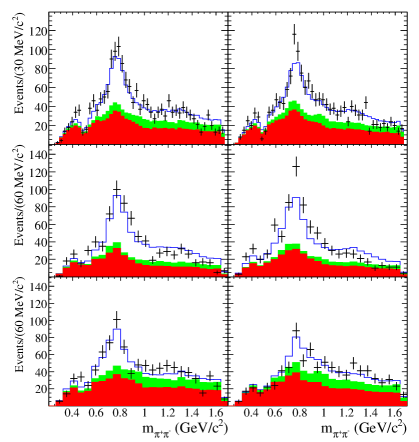
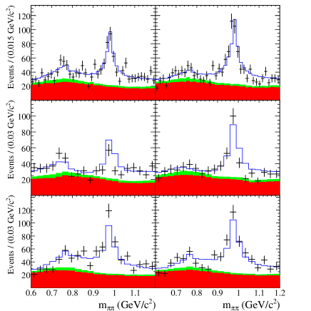
Understanding the origin of these $C\!P$ violation effects requires related modes to also be studied. The Laura⁺⁺ package has also been used by the BaBar collaboration for a time-dependent DP analysis of ${{B}^{0}}\rightarrow{{K}^{0}_{\rm\scriptscriptstyle S}}{{\pi}^{+}}{{\pi}^{-}}$ decays [44], as well as for an amplitude analysis of $B^{+}\rightarrow{{K}^{0}_{\rm\scriptscriptstyle S}}\pi^{+}\pi^{0}$ decays [86]. In the latter, the modelling of the large background contribution, as well as of the smearing of the DP position due to the limited resolution of the neutral pion momentum (self cross-feed), is particularly important. In addition, correlations between the DP position and the variables that are used to discriminate signal decays from background contributions are taken into account as described in App. D.13. The amplitude model includes components from the $K^{*}(892)$ resonance and $K\pi$ S-wave (both appearing in both charged and neutral channels) as well as the $\rho(770)^{+}$ resonance. Projections of the fit results are shown in Fig. 6. The analysis reveals evidence for a $C\!P$ asymmetry in ${{{B}^{+}}}\rightarrow K^{*}(892)^{+}{{\pi}^{0}}$ decays.

Figure 6: Projections of the data and fit results onto (top) ${{K}^{0}_{\rm\scriptscriptstyle S}}{{\pi}^{\mp}}$, (middle) ${{K}^{0}_{\rm\scriptscriptstyle S}}{{\pi}^{0}}$ and (bottom) ${{\pi}^{\mp}}{{\pi}^{0}}$ invariant mass distributions for ${{{B}^{+}}}\rightarrow{{K}^{0}_{\rm\scriptscriptstyle S}}{{\pi}^{+}}{{\pi}^{0}}$ candidates observed by the BaBar collaboration [86]. Background from ${{D}^{0}}\rightarrow{{K}^{0}_{\rm\scriptscriptstyle S}}{{\pi}^{0}}$ has been vetoed. In each row the left (right) plot is for $B^{-}$ ($B^{+}$) candidates. The data are the points with error bars, the (black) dash-dotted curves represent the signal contribution, the dotted (red) curves to the continuum background component, the dashed (green) curves to the total background contribution and the solid (blue) curves the total fit result.

The LHCb collaboration has used the Laura⁺⁺ package for several studies of multibody $B$ meson decays to charmed final states, with important results for charm spectroscopy and $C\!P$ violation measurements. For example, the ${{B}^{0}_{s}}\rightarrow{{\kern 1.99997pt\overline{\kern-1.99997ptD}{}}{}^{0}}{{K}^{-}}{{\pi}^{+}}$ decay was found to have a DP structure that contains effects from overlapping spin-1 and spin-3 resonances with masses around $m({{\kern 1.99997pt\overline{\kern-1.99997ptD}{}}{}^{0}}{{K}^{-}})\sim 2.86{\mathrm{\,Ge\kern-1.00006ptV\!/}c^{2}}$ [87, 88]. The neutral charm meson is reconstructed through its ${{\kern 1.99997pt\overline{\kern-1.99997ptD}{}}{}^{0}}\rightarrow{{K}^{+}}{{\pi}^{-}}$ decay. The model contains contributions from the ${{\kern 1.99997pt\overline{\kern-1.99997ptK}{}}{}^{*}}(892)^{0}$, ${{\kern 1.99997pt\overline{\kern-1.99997ptK}{}}{}^{*}}(1410)^{0}$, ${\kern 1.99997pt\overline{\kern-1.99997ptK}{}}{}^{*}_{2}(1430)^{0}$, ${{\kern 1.99997pt\overline{\kern-1.99997ptK}{}}{}^{*}}(1680)^{0}$ resonances as well as a ${{K}^{-}}{{\pi}^{+}}$ S-wave component, and $D_{s2}^{*}(2573)^{-}$, $D_{s1}^{*}(2700)^{-}$, $D_{s1}^{*}(2860)^{-}$, $D_{s3}^{*}(2860)^{-}$ resonances together with a nonresonant ${{\kern 1.99997pt\overline{\kern-1.99997ptD}{}}{}^{0}}{{K}^{-}}$ S-wave amplitude and virtual contributions from the $D_{s\,v}^{*-}$, $D_{s0\,v}^{*}(2317)^{-}$ and $B_{v}^{*+}$ states. The results of the analysis include the first experimental proof of the spin-2 nature of the $D_{s2}^{*}(2573)^{-}$ state, as well as world-leading measurements of the masses and widths of many of the resonances. Projections of the DP fit results onto the data are shown in Fig. 7.

Figure 7: Projections of the data and fit results onto (top left) ${{K}^{-}}{{\pi}^{+}}$ and (top right) ${{\kern 1.99997pt\overline{\kern-1.99997ptD}{}}{}^{0}}{{K}^{+}}$ invariant mass distributions for ${{B}^{0}_{s}}\rightarrow{{\kern 1.99997pt\overline{\kern-1.99997ptD}{}}{}^{0}}{{K}^{-}}{{\pi}^{+}}$ candidates observed by the LHCb collaboration [87, 88]. Background from ${{D}^{0}}\rightarrow{{K}^{-}}{{\pi}^{+}}$ has been vetoed. A legend describing the various contributions is also given, together with (bottom left) a zoom around $m({{\kern 1.99997pt\overline{\kern-1.99997ptD}{}}{}^{0}}{{K}^{-}})\sim 2.86{\mathrm{\,Ge\kern-1.00006ptV\!/}c^{2}}$ and (bottom right) a projection onto the cosine of the helicity angle $\theta({{\kern 1.99997pt\overline{\kern-1.99997ptD}{}}{}^{0}}{{K}^{-}})$ for candidates in that region. In the last case, projections of the results of fits with models containing either or both of the $D_{s1}^{*}(2860)^{-}$ and $D_{s3}^{*}(2860)^{-}$ resonances are shown, demonstrating the need for both to obtain a good fit to the data.

A similar DP analysis with the Laura⁺⁺ package has been performed by the LHCb collaboration for the ${{B}^{0}}\rightarrow{{\kern 1.99997pt\overline{\kern-1.99997ptD}{}}{}^{0}}{{K}^{+}}{{\pi}^{-}}$ mode [89]. The model obtained is an essential input into a subsequent analysis of the same decay with the neutral charm meson reconstructed through $D$ decays to the $C\!P$ eigenstates ${{K}^{+}}{{K}^{-}}$ and ${{\pi}^{+}}{{\pi}^{-}}$ [70]. In the latter case, contributions from both ${{B}^{0}}\rightarrow{{D}^{0}}{{K}^{+}}{{\pi}^{-}}$ and ${{\kern 1.99997pt\overline{\kern-1.99997ptD}{}}{}^{0}}{{K}^{+}}{{\pi}^{-}}$ amplitudes can interfere, giving sensitivity to the angle $\gamma$ of the CKM unitarity triangle. A DP analysis allowing for $C\!P$ violation effects provides a powerful way to determine $\gamma$ without ambiguities [51, 52]. In this analysis, a simultaneous fit to the final states with different $D$ decays is implemented using the Jfit method described in Sec. 7.3.7 and Ref. [71]. Projections of the fit result onto the data (weighted by the signal purity) are shown in Fig. 8. No significant $C\!P$ violation effect is observed, and the resulting limits on $\gamma$ are not strongly constraining. The method is, however, expected to give competitive constraints on $\gamma$ as larger data samples become available and as additional $D$ meson decay modes are included in the analysis. Moreover, the analysis also gives results for hadronic parameters that must be known in order to interpret results from quasi-two-body analyses of ${{B}^{0}}\rightarrow D{{K}^{*}}(892)^{0}$ decays in terms of $\gamma$. As such, the results have an important impact in combinations of results to obtain the best knowledge of $\gamma$ [90, 91].

Figure 8: Projections of the data and fit results onto $m({{K}^{\mp}}{{\pi}^{\pm}})$ for (left) ${{\kern 1.79993pt\overline{\kern-1.79993ptB}{}}{}^{0}}\rightarrow D{{K}^{-}}{{\pi}^{+}}$ and (right) ${{B}^{0}}\rightarrow D{{K}^{+}}{{\pi}^{-}}$ candidates observed by the LHCb collaboration [70]. A legend describing the various contributions is also given.

Other decays of the type $B\rightarrow D^{(*)}K\pi$ have sensitivity to $\gamma$, and are also important to study as possible background contributions to the two-body $B\rightarrow D^{(*)}K$ type decays that are more conventionally used for this purpose. The LHCb collaboration has also published results on the ${{{B}^{+}}}\rightarrow{{D}^{-}}{{K}^{+}}{{\pi}^{+}}$ [92] and ${{D}^{+}}{{K}^{+}}{{\pi}^{-}}$ [93] decays, which were obtained from analyses using the Laura⁺⁺ package. The higher-yield $B\rightarrow D^{(*)}\pi\pi$ channels provide some of the most interesting possibilities to explore charm spectroscopy. An amplitude analysis of ${{{B}^{+}}}\rightarrow{{D}^{-}}{{\pi}^{+}}{{\pi}^{+}}$ [94] has been performed by the LHCb collaboration, using the Laura⁺⁺ package, in which the model contains contributions from the ${\kern 1.99997pt\overline{\kern-1.99997ptD}{}}{}_{2}^{*}(2460)^{0}$, ${\kern 1.99997pt\overline{\kern-1.99997ptD}{}}{}_{1}^{*}(2760)^{0}$, ${\kern 1.99997pt\overline{\kern-1.99997ptD}{}}{}_{3}^{*}(2760)^{0}$ and ${\kern 1.99997pt\overline{\kern-1.99997ptD}{}}{}_{2}^{*}(3000)^{0}$ resonances (the last three of which are either confirmed or observed for the first time), as well as virtual contributions from the ${\kern 1.99997pt\overline{\kern-1.99997ptD}{}}{}_{v}^{*}(2007)^{-}$ and $B_{v}^{*0}$ states. In the absence of sufficiently detailed models for the ${{D}^{-}}{{\pi}^{+}}$ S-wave, a quasi-model-independent description based on spline interpolation is used. Projections of the results of the fit onto the data are shown in Fig. 9.

Figure 9: Projections of the data and fit results onto $m({{D}^{-}}{{\pi}^{+}})_{\rm min}$ for ${{{B}^{+}}}\rightarrow{{D}^{-}}{{\pi}^{+}}{{\pi}^{+}}$ candidates observed by the LHCb collaboration [94] on (top left) linear and (bottom right) logarithmic $y$-axis scales. Here, $m({{D}^{-}}{{\pi}^{+}})_{\rm min}$ is the smaller of the two values of $m({{D}^{-}}{{\pi}^{+}})$ for each ${{{B}^{+}}}\rightarrow{{D}^{-}}{{\pi}^{+}}{{\pi}^{+}}$ candidate. A legend describing the various contributions is also given. The (bottom right) Argand diagram of the ${{D}^{-}}{{\pi}^{+}}$ S-wave amplitude shows the expected phase motion corresponding to the ${\kern 1.99997pt\overline{\kern-1.99997ptD}{}}{}_{0}^{*}(2400)^{0}$ resonance. The numbered points correspond to the spline knots.

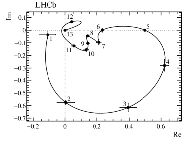
8.3 Speed

It is essential for the Laura⁺⁺ amplitude analysis package to run quickly, since otherwise the large data samples available in modern experiments can lead to unmanageably long execution time. In this subsection some performance benchmarks are provided. More specifically, a selection of the examples that are provided with the package (several of which are based on analyses presented in the previous subsection) are run out of the box on the same machine (an Intel Core i5-3570 3.4${\rm\,GHz}$ quad-core CPU with 8${\rm\,Gbytes}$ of RAM). In each case, timings for both generation of 50 toy datasets and for fitting those same 50 datasets are provided in Table 3. The fitting times are averaged over 20 fits with randomised starting parameters. The scenario demonstrated in each example is as follows:

• GenFit3pi.cc
  Example analysis of the symmetric final state ${{{B}^{+}}}\rightarrow{{\pi}^{+}}{{\pi}^{+}}{{\pi}^{-}}$, using LauSimpleFitModel (i.e. not including effects of $C\!P$ violation). By default there are 1500 signal events per experiment and the signal isobar model contains five components: $\rho(770)^{0}$, $f_{0}(980)$, $f_{2}(1270)$, $\rho(1450)^{0}$, and a nonresonant component. All of the resonance parameters are fixed in the fit. There is also a background component, which defaults to being uniformly distributed in the Dalitz plot and consists of 1250 background events. A version of this example implemented in python, GenFit3pi.py, is also included in the Laura⁺⁺ package.

• GenFit3K.cc
  Example analysis of the symmetric final state ${{{B}^{+}}}\rightarrow{{K}^{+}}{{K}^{+}}{{K}^{-}}$, using LauSimpleFitModel (i.e. not including effects of $C\!P$ violation). By default there are 5000 signal events per experiment and the signal isobar model contains three components: $\phi(1020)$, $f_{2}^{\prime}(1525)$ and a nonresonant component. The mass and width of both the $\phi(1020)$ and the $f_{2}^{\prime}(1525)$ are floating parameters by default and a two-stage fit is employed. No background contributions are included. To demonstrate further the impact on the performance of floating resonance parameters, this example is run with:

  • no floating resonance parameters,

  • only the mass of the $\phi(1020)$ floating,

  • the mass and width of the $\phi(1020)$ floating,

  • the mass and width of both the $\phi(1020)$ and $f^{\prime}_{2}(1525)$ floating,

  and the timings for each of those scenarios are provided in Table 4.

• GenFit3KS.cc
  Example analysis of the fully-symmetric final state ${{B}^{0}}\rightarrow{{K}^{0}_{\rm\scriptscriptstyle S}}{{K}^{0}_{\rm\scriptscriptstyle S}}{{K}^{0}_{\rm\scriptscriptstyle S}}$, using LauSimpleFitModel (i.e. not including effects of $C\!P$ violation). By default there are 10000 signal events per experiment and the signal isobar model contains four components: $f_{0}(980)$, $f_{0}(1710)$, $f_{2}(2010)$ and ${\chi_{{c}0}}$. All of the resonance parameters are fixed in the fit. No background contributions are included.

• GenFitDs2KKpi.cc
  Example analysis of the decay ${{D}^{+}_{s}}\rightarrow{{\pi}^{+}}{{K}^{+}}{{K}^{-}}$, using LauSimpleFitModel (i.e. not including effects of $C\!P$ violation). By default there are 10000 signal events and the signal isobar model contains three components: $\phi(1020)$, ${{K}^{*}}(892)^{0}$ and a nonresonant component. All of the resonance parameters are fixed in the fit. No background contributions are included.

• GenFitEFKLLM.cc
  Example analysis of the decay ${{B}^{0}}\rightarrow{{\kern 1.99997pt\overline{\kern-1.99997ptD}{}}{}^{0}}{{K}^{+}}{{\pi}^{-}}$, using LauSimpleFitModel (i.e. not including effects of $C\!P$ violation). By default there are 5000 signal events per experiment and the signal isobar model contains two components, which are the two parts of the EFKLLM model for the ${{K}^{+}}{{\pi}^{-}}$ S-wave (see Eq. (52) in App. A). This example mainly serves to demonstrate how to use this particular model.

• GenFitBelleCPKpipi.cc
  Example analysis of the decay ${{{B}^{+}}}\rightarrow{{K}^{+}}{{\pi}^{+}}{{\pi}^{-}}$, using LauCPFitModel, which includes effects from $C\!P$ violation. By default there are 5000 signal events per experiment and the signal isobar model contains seven components: ${{K}^{*}}(892)^{0}$, ${K}^{*}_{0}(1430)^{0}$, $\rho(770)^{0}$, $f_{0}(980)$, $\chi_{{c}0}$, and two nonresonant components. The slope of the ${{\pi}^{+}}{{\pi}^{-}}$ exponential nonresonant model and the effective range and scattering length of the ${{K}^{+}}{{\pi}^{-}}$ LASS nonresonant component are floating parameters by default. The isobar coefficients use the LauBelleCPCoeffSet form to parameterise the $C\!P$ violation (see Table 1) and a two-stage fit is employed. No background contributions are included.

• GenFitKpipi.cc
  Example analysis of the decay ${{{B}^{+}}}\rightarrow{{K}^{+}}{{\pi}^{+}}{{\pi}^{-}}$, using LauCPFitModel, which includes effects from $C\!P$ violation. This example is based closely on the BaBar analysis from Ref. [36]. By default there are 4585 signal events per experiment and the signal isobar model contains seven components: ${{K}^{*}}(892)^{0}$, ${K}^{*}_{0}(1430)^{0}$, ${K}^{*}_{2}(1430)^{0}$, $\rho(770)^{0}$, $\omega(782)$, $f_{0}(980)$, $f_{2}(1270)$, $f^{\prime}_{0}(1300)$, $\chi_{{c}0}$, and a nonresonant component. All of the resonance parameters are fixed in the fit. The isobar coefficients use the LauCartesianCPCoeffSet form to parameterise the $C\!P$ violation (see Table 1) and a two-stage fit is employed. Background contributions for combinatorial candidates and those from other $B$ decays are included.

• KMatrixExample.cc and KMatrixDto3pi.cc
  These examples demonstrate how to use the K-matrix description of the S-wave. The first scenario is for the ${{B}^{0}}\rightarrow{{\pi}^{+}}{{\pi}^{-}}{{K}^{0}_{\rm\scriptscriptstyle S}}$ DP but the only terms included in the signal model are $\rho(770)^{0}$, ${{K}^{*}}(892)^{+}$ and a K-matrix component for the ${{\pi}^{+}}{{\pi}^{-}}$ S-wave. By default there are 5000 signal events per experiment. The second scenario is for the symmetric ${{D}^{+}}\rightarrow{{\pi}^{+}}{{\pi}^{+}}{{\pi}^{-}}$ DP and includes in the signal model the $\rho(770)^{0}$, $f_{2}(1270)$, and the K-matrix. By default there are 20000 signal events per experiment. In both scenarios there are no background contributions and all resonance parameters are fixed in the fit.

• GenFitNoDP.cc and GenFitNoDPMultiDim.cc
  These examples demonstrate how to use the package to perform fits to variables other than the DP. The first case fits only a single variable (the invariant mass of the ${{B}^{+}}$ candidate), while the second performs a 2D fit. In both cases there are 5000 signal events. In the first case there are two background components included, which have yields of 7000 and 3000 events. In the second case there is a single background component that has a yield of 7000 events. All yield parameters are floating, along with some of the shape parameters of the PDFs. Asymmetric uncertainties are evaluated in the first case.

• runMasterSlave.sh, Master.cc and Slave.cc
  This example demonstrates how to perform a simultaneous fit to two categories of data in the decay channel ${{B}^{0}}\rightarrow{{\pi}^{0}}{{\pi}^{0}}{{K}^{0}_{\rm\scriptscriptstyle S}}$. The data are split based on the reconstruction category of the ${K}^{0}_{\rm\scriptscriptstyle S}$ candidate. In one category there are 500 signal and 1200 background events, while in the second there are 750 signal and 2500 background events. The common signal DP model contains contributions from the $f_{0}(980)$, $f_{2}(1270)$, ${{K}^{*}}(892)^{0}$, and ${K}^{*}_{0}(1430)^{0}$ resonances. The mass of the ${{K}^{*}}(892)^{0}$ resonance is a floating parameter of the fit and a two-stage fit is employed. The background component is distributed uniformly in the DP by default. To demonstrate further the impact on the performance of simultaneous fitting, this example is run with:

  • the Master and the two Slave processes all running on the same host,

  • the Master and the two Slave processes running on three separate hosts,

  and the timings for each of these scenarios are provided in Table 5. To run this particular example, the hosts have dual Intel Xeon E5-2620v2 2.1${\rm\,GHz}$ 6-core CPUs and 64${\rm\,Gbytes}$ of RAM and are connected via 10${\rm\,Gbits/s}$ ethernet.

Table 3: Speed of execution of the examples provided with the Laura⁺⁺ package. The times given are the total to generate/fit 50 toy experiments. The examples differ, as explained in detail in the text, not only through the complexity of the model but also through the number of signal and background events in each pseudoexperiment.

Example	Execution time of	Execution
	toy generation	time of fit
GenFit3pi.cc	$7\rm{\,s}$	$9\rm{\,s}$
GenFit3K.cc	$291\rm{\,s}$	$2513\rm{\,s}$
GenFit3KS.cc	$78\rm{\,s}$	$20\rm{\,s}$
GenFitDs2KKpi.cc	$47\rm{\,s}$	$9\rm{\,s}$
GenFitEFKLLM.cc	$106\rm{\,s}$	$3\rm{\,s}$
GenFitBelleCPKpipi.cc	$14\rm{\,s}$	$18909\rm{\,s}$
GenFitKpipi.cc	$36\rm{\,s}$	$1073\rm{\,s}$
KMatrixExample.cc	$194\rm{\,s}$	$217\rm{\,s}$
KMatrixDto3pi.cc	$46\rm{\,s}$	$251\rm{\,s}$
GenFitNoDP.cc	$2\rm{\,s}$	$11\rm{\,s}$
GenFitNoDPMultiDim.cc	$3\rm{\,s}$	$6\rm{\,s}$

Table 4: Speed of execution of the GenFit3K.cc example provided with the Laura⁺⁺ package with different sets of floating resonance parameters. The times given are the total to fit 50 toy experiments.

Floated parameters	Execution time of fit
None	$6\rm{\,s}$
Mass of $\phi(1020)$	$702\rm{\,s}$
Mass and width of $\phi(1020)$	$1090\rm{\,s}$
Mass and width of $\phi(1020)$ and $f^{\prime}_{2}(1525)$	$2513\rm{\,s}$

Table 5: Speed of execution of the fitting portion of the runMasterSlave.sh example provided with the Laura⁺⁺ package with the Master and two Slave processes running either on the same or separate hosts. The times given are the total to fit 50 toy experiments.

Host setup	Execution time of fit
Master and two Slave processes on single host	$1972\rm{\,s}$
Master and two Slave processes on three separate hosts	$2151\rm{\,s}$

9 Future developments

There are several features that would help to improve and extend the functionality of Laura⁺⁺ in the future. Some of these potential future developments are described below. In addition, it is anticipated that the Laura⁺⁺ code will be continually updated to take advantage of features in the latest C++ standards.

9.1 Plotting the amplitude

Currently the user can easily make plots of the DP distribution or its projections from the result of the fit (see Sec. 7.2). It can also be of interest to draw amplitude-level quantities, for example to show the phase variation with two-body invariant mass of a particular partial wave. While this is currently possible in Laura⁺⁺ (see Fig. 9 for an example), it would be desirable to provide an interface to simplify matters for the user.

9.2 Decay-time-dependent fits

As mentioned in Sec. 1, the evolution of DP structure with decay time of a $B$ or $D$ meson can be of interest to study $C\!P$ violation effects. For example, studies of ${{B}^{0}}\rightarrow{{\pi}^{+}}{{\pi}^{-}}{{\pi}^{0}}$ and $D{{\pi}^{+}}{{\pi}^{-}}$ decays are of interest to measure the angles $\alpha$ and $\beta$ of the CKM Unitarity Triangle with low theoretical uncertainty. Studies of ${{B}^{0}}\rightarrow{{K}^{0}_{\rm\scriptscriptstyle S}}{{\pi}^{+}}{{\pi}^{-}}$ and ${{K}^{0}_{\rm\scriptscriptstyle S}}{{K}^{+}}{{K}^{-}}$ decays enable determinations of $\beta$ that are not as clean, but are potentially sensitive to effects of physics beyond the Standard Model. Also, the ${{D}^{0}}\rightarrow{{K}^{0}_{\rm\scriptscriptstyle S}}{{\pi}^{+}}{{\pi}^{-}}$ channel appears the most sensitive to possible $C\!P$ violation effects associated with charm mixing. Many other channels are potentially of interest.

The Laura⁺⁺ package has been used for decay-time-dependent DP analysis, for example, in Refs. [44, 50]. However, this implementation was experiment-specific and therefore unsuitable for use in the more general case. Further development is necessary to establish a model that can deal generically with issues such as flavour tagging, decay time resolution and acceptance as well as production and detection asymmetries.

9.3 Alternative handling of resolution effects

The treatment of resolution discussed in Sec. 3 and Sec. 5.2 is completely general, but is likely to be inefficient in certain cases. For example, in the ${{{B}^{+}}}\rightarrow{{K}^{+}}{{K}^{-}}{{K}^{+}}$ decay, there are narrow contributions from the $\phi(1020)$ and $\chi_{c0}$ resonances in specific regions of the DP, for which resolution effects may be important. The rest of the DP is populated with broad or nonresonant states so that resolution can be safely neglected. An approach in which Gaussian (or non-Gaussian) smearing of Dalitz plot position can be used in only selected regions of the phase space may be useful. In such a case it will be necessary to take care to avoid issues due to edge effects, including the possibility of an event being smeared to positions outside the kinematic boundary of the DP.

9.4 Non-zero spins

There are many interesting three-body decays that include particles with non-zero spin in the initial and final states, which cannot be fitted using the current version of Laura⁺⁺. Large samples of $b$-baryons are available in the LHCb data samples, which have baryons in the initial and final states, for example ${{\mathchar 28931\relax}^{0}_{b}}\rightarrow{{\kern 1.99997pt\overline{\kern-1.99997ptD}{}}{}^{0}}{p}{{\pi}^{-}}$ and ${{\mathchar 28932\relax}^{-}_{b}}\rightarrow{p}{{K}^{-}}{{K}^{-}}$ decays. Decays of ${B}\rightarrow{{J\mskip-3.0mu/\mskip-2.0mu\psi\mskip 2.0mu}}hh^{\prime}$, where $h$ and $h^{\prime}$ are charged pions or kaons, are also interesting and contain the spin-1 ${{J\mskip-3.0mu/\mskip-2.0mu\psi\mskip 2.0mu}}$ particle. Another group of decay modes, ${B}\rightarrow{{D}^{*}}hh^{\prime}$, which include the vector ${D}^{*}$ meson, are interesting for spectroscopy of $D^{**}$ and $D_{s}^{**}$ states.

To enable the Laura⁺⁺ package to cope with the decays above, several things would require updating or changing. Firstly, the phase space of the problem is expanded from two to five dimensions where additional degrees of freedom would be some angular variables. The helicity of particles of non-zero spin, like the ${{J\mskip-3.0mu/\mskip-2.0mu\psi\mskip 2.0mu}}$, must also be considered, requiring a sum over the helicity states. For the initial and final state this sum must be incoherent and for the intermediate states a coherent sum is required. The Zemach spin terms currently implemented must also be changed for the non-zero spin particles. One potential way to calculate the spin factors would be to interface Laura⁺⁺ with the qft++ package [95], which allows the spin terms to be calculated for any process.

9.5 Genetic algorithms

To ensure that the global minimum in the NLL has been found, Laura⁺⁺ allows many fits to be performed with randomised starting values for the floated fit parameters. This method works well, but can become time consuming if the global minimum is not found in a high proportion of fit attempts. Genetic algorithms could provide a method to find sensible starting values for the floated parameters such that the global minimum is always found. This could be achieved by interfacing to existing software packages with implementations of genetic algorithms.

9.6 Interface to EvtGen

The EvtGen package [96] is designed to predominantly simulate the decays of $b$- and $c$-hadrons. It is important in experimental particle physics to produce simulated data samples that are realistic and match the true data samples. Typically in three-body decays the simulated events are produced flat in the DP, without resonant contributions. It would be beneficial if Laura⁺⁺ could be used directly to provide realistic DP distributions for simulated samples of three-body decays.

10 Summary

The Laura⁺⁺ package provides a flexible and optimised framework for Dalitz-plot analysis. While it can be used for the decay of any stable spin-zero particle to any final state containing three stable spin-zero particles, it has until now been most widely used for decays of $B$ or $D$ mesons to three pseudoscalars. Features included in Laura⁺⁺ allow the physics of such decays to be probed in detail, including studies of the resonances appearing in the contributing partial waves, and investigations of $C\!P$-violating effects. Use of the Laura⁺⁺ software has resulted in numerous publications to date, with many more expected in future with the increasingly large data samples available at LHCb, Belle II and other experiments.

11 Acknowledgements

The Laura⁺⁺ package has been under development for many years, with support principally from the Science and Technology Facilities Council (United Kingdom) and by the European Research Council under FP7. Individual authors have received support from Marie Skłodowska-Curie Actions and from the University of Warwick. We thank the Laura⁺⁺ user community for feedback, bug reports, testing and other contributions to improve the package, in particular Louis Henry, Adlene Hicheur, Patricia Magalhães, Jussara Miranda, Sian Morgan and Charlotte Wallace. We also acknowledge productive discussions regarding aspects of Dalitz plot analysis with many members of the BaBar, Belle and LHCb collaborations, notably Eli Ben-Haim, Alex Bondar, Jeremy Dalseno, Bill Dunwoodie, Brian Meadows and Anton Poluektov. Similarly, instructive communications with members of the theory community have been of great benefit; in particular we thank Vladimir Anisovich, David Bugg, Leonard Lesniak, Benoit Loiseau, Mike Pennington, Alessandro Pilloni, Andrey Sarantsev and Adam Szczepaniak. Furthermore, we thank Bertram Kopf and Matthias Steinke for providing access to the PAWIAN software (PANDA collaboration) for cross-checking the $K$-matrix implementation. Finally, we acknowledge useful input on technical features of the package from René Brun and Bertrand Echenard.

Appendices

Appendix A Formulae for available lineshapes

This section presents the complete formulae for all resonance shapes implemented in Laura⁺⁺. Table A1 gives the list of shapes, together with the corresponding LauResonanceModel enumeration integer that is required to specify the resonance type for the LauIsobarDynamics addResonance function, as well as the equation number(s) that provide the expression for the resonance mass term $R(m)$ used in Eq. (4). The K-matrix shape is particularly complicated and is therefore described in a dedicated subsection.

Table A1: List of the allowed resonance shape types. The LauResonanceModel case-sensitive enumeration in the LauAbsResonance abstract class specifies the integer that selects the resonance type for the addResonance function. For example, the simple Breit–Wigner integer type is LauAbsResonance::BW.

Shape name	Enumeration	$R(m)$ Eq.
Simple Breit–Wigner	BW	(37)
Relativistic Breit–Wigner (RBW)	RelBW	(6)
Modified Breit–Wigner from Gounaris–Sakurai (GS)	GS	(39)
Flatté or coupled-channel Breit–Wigner	Flatte	(44)
$\sigma$ or $f_{0}(500)$	Sigma	(47)
$\kappa$ or low-mass $K\pi$ scalar	Kappa	(47)
Low-mass $D\pi$ scalar	Dabba	(49)
LASS $K\pi$ S-wave	LASS	(50)
Resonant part of $K\pi$ LASS	LASS_BW	(50) (2nd term)
Non-resonant part of $K\pi$ LASS	LASS_NR	(50) (1st term)
Form-factor description of the $K\pi$ S-wave	EFKLLM	(52)
S-wave using $K$-matrix and $P$-vector	KMatrix	(70)–(76)
Uniform non-resonant (NR)	FlatNR	$R(m)\equiv 1$
Theoretical NR model	NRModel	(53)
Empirical NR exponential	BelleNR	(55)
Empirical NR power-law	PowerLawNR	(56)
Empirical NR exponential for symmetrised DPs	BelleSymNR	(57)
Empirical NR Taylor expansion for symmetrised DPs	TaylorNR	(58)
Empirical NR polynomial	PolNR	(59)
Model-independent partial wave (magnitude & phase)	MIPW_MagPhase	(61)
Model-independent partial wave (real & imaginary)	MIPW_RealImag	(61)
Incoherent Gaussian shape	GaussIncoh	(62)
$\rho-\omega$ mixing: GS for $\rho$, RBW for $\omega$	RhoOmegaMix_GS	(60)
neglecting $\Delta^{2}$ denominator term	RhoOmegaMix_GS_1	(60)
$\rho-\omega$ mixing: RBW for both $\rho$ and $\omega$	RhoOmegaMix_RBW	(60)
neglecting $\Delta^{2}$ denominator term	RhoOmegaMix_RBW_1	(60)

The simple Breit–Wigner lineshape is given by

$$R(m)=\frac{1}{m-m_{0}-\frac{i}{2}\Gamma_{0}}\equiv\frac{(m-m_{0})+\frac{i}{2}\Gamma_{0}}{(m-m_{0})^{2}+\frac{\Gamma^{2}_{0}}{4}}\,,$$ (37)

where $m_{0}$ is the pole mass and $\Gamma_{0}$ is the resonance width. The more commonly used relativistic Breit–Wigner lineshape is described in Sec. 2.1. We note here that the relativistic Breit–Wigner lineshape can also describe so-called virtual contributions, from resonances with masses outside the kinematically accessible region of the Dalitz plot, with one modification: in the calculation of the momenta, the mass $m_{0}$ is set to a value $m_{0}^{\rm{eff}}$ within the kinematically allowed range. This is accomplished with the ad-hoc formula

$$m_{0}^{\rm{eff}}(m_{0})=m^{\rm{min}}+\frac{1}{2}(m^{\rm{max}}-m^{\rm{min}})\left[1+\tanh\left(\frac{m_{0}-\frac{m^{\rm{min}}+m^{\rm{max}}}{2}}{m^{\rm{max}}-m^{\rm{min}}}\right)\right]\,,$$ (38)

where $m^{\rm{max}}$ and $m^{\rm{min}}$ are the upper and lower limits of the kinematically allowed mass range. For virtual contributions, only the tail of the RBW function enters the Dalitz plot.

The Gounaris–Sakurai form of the Breit–Wigner lineshape [97] is usually used as an alternative model for the $\rho$ resonance. It is given by

$$R(m)=\frac{1+D\cdot\Gamma_{0}/m_{0}}{(m_{0}^{2}-m^{2})+f(m)-i\,m_{0}\Gamma(m)}\,,$$ (39)

where

$$f(m)=\Gamma_{0}\,\frac{m_{0}^{2}}{q_{0}^{3}}\,\left[\;q^{2}\left[h(m)-h(m_{0})\right]+\left(\,m_{0}^{2}-m^{2}\,\right)\,q^{2}_{0}\,\frac{dh}{ds}\bigg{|}_{m_{0}}\;\right]\,,$$ (40)

$q$ is the magnitude of the momentum of one of the daughter particles in the resonance rest-frame,

$$h(m)=\frac{2}{\pi}\,\frac{q}{m}\,\ln\left(\frac{m+2q}{2m_{\pi}}\right)\,,$$ (41)

and

$$\frac{dh}{ds}\bigg{|}_{m_{0}}=h(m_{0})\left[(8q_{0}^{2})^{-1}-(2m_{0}^{2})^{-1}\right]\,+\,(2\pi m_{0}^{2})^{-1}\,.$$ (42)

The constant parameter $D$ is given by [97]

$$D=\frac{3}{\pi}\frac{m_{\pi}^{2}}{q_{0}^{2}}\,\ln\left(\frac{m_{0}+2q_{0}}{2m_{\pi}}\right)+\frac{m_{0}}{2\pi\,q_{0}}-\frac{m_{\pi}^{2}m_{0}}{\pi\,q_{0}^{3}}\,.$$ (43)

The Flatté [98], or coupled two-channel Breit–Wigner, lineshape is usually used to model $f_{0}(980)$, $K^{*}_{0}(1430)$ and $a_{0}(980)$ states. It was originally introduced in the form

$$R(m)=\frac{1}{(m_{0}^{2}-m^{2})-im_{0}[\Gamma_{1}(m)+\Gamma_{2}(m)]}\,.$$ (44)

The decay widths in the two systems are usually represented by products of couplings and dimensionless phase-space factors:

$$\Gamma_{1}(m)=g_{1}f_{A}\left(\frac{1}{3}\sqrt{1-(m_{1,1}+m_{1,2})^{2}/m^{2}}+\frac{2}{3}\sqrt{1-(m_{1,3}+m_{1,4})^{2}/m^{2}}\right)\,,$$ (45)

$$\Gamma_{2}(m)=g_{2}f_{A}\left(\frac{1}{2}\sqrt{1-(m_{2,1}+m_{2,2})^{2}/m^{2}}+\frac{1}{2}\sqrt{1-(m_{2,3}+m_{2,4})^{2}/m^{2}}\right)\,.$$ (46)

Here the fractional coefficients come from isospin conservation, $m_{i,j}$ denotes the invariant mass of the daughter particle $j$ (1–4) in channel $i$ (1–2), and $g_{1}$ and $g_{2}$ are coupling constants whose values are assumed to be those provided in Table A2. The Clebsch-Gordan coefficients in Eqs. 45 and 46 are not guaranteed to be correct for every possible resonance that could be modelled with the Flatté lineshape, but are appropriate for every case considered in Table A2. The expressions for the widths are continued analytically ($\Gamma\rightarrow i|\Gamma|$) when $m$ is below any of the specific channel thresholds, contributing to the real part of the amplitude, while the Adler-zero term $f_{A}=(m^{2}-s_{A})/(m^{2}_{0}-s_{A})$ can be used to suppress false kinematic singularities when $m$ goes below threshold [99] (otherwise $f_{A}$ is set to unity).

Variants of the Flatté lineshape have been used in the literature. In some cases, e.g. Refs. [100, 101], the constant $m_{0}$ that multiplies the widths in the denominator of Eq. (44) is absorbed into the couplings. As a consequence the couplings have dimensions of mass-squared, and are sometimes denoted as $g_{i}$ [100] and sometimes as $g_{i}^{2}$ [101]. In Table A2 all values have been converted to be consistent with Eqs. (44)–(46). In Laura⁺⁺ it is only possible to use the Flatté lineshape for the systems specified in Table A2. At construction time the resonance name is checked and the corresponding parameter values are set; these can be modified by the user if desired.

Table A2: The four daughter particles used for each channel term $m_{ij}$, as well as the coupling ($g_{1}$, $g_{2}$) and Adler-zero ($s_{A}$) constants for the Flatté lineshapes. Units of $\mathrm{\,Ge\kern-1.00006ptV}$ for $g_{1,2}$ (or $\mathrm{\,Ge\kern-1.00006ptV}^{2}$ for $m_{0}g_{1,2}$ when taken from Refs. [100, 101]) and ${\mathrm{\,Ge\kern-1.00006ptV^{2}\!/}c^{4}}$ for $s_{A}$ are implied.

Resonance	Channel 1	Channel 2	$g_{1}$ or $m_{0}g_{1}$	$g_{2}$ or $m_{0}g_{2}$	$s_{A}$	Reference
$f_{0}(980)$	${\pi}^{0}$,${\pi}^{0}$,${\pi}^{\pm}$,${\pi}^{\pm}$	${K}^{\pm}$,${K}^{\pm}$,${K}^{0}$,${K}^{0}$	0.165	$4.21g_{1}$	—	[100]
$K^{*}_{0}(1430)^{0}$	${K}^{0}$,${\pi}^{0}$,${K}^{\pm}$,${\pi}^{\pm}$	${K}^{0}$,$\eta^{\prime}$,${K}^{0}$,$\eta^{\prime}$	0.304	0.380	0.234	[99]
$K^{*}_{0}(1430)^{\pm}$	${K}^{\pm}$,${\pi}^{0}$,${K}^{0}$,${\pi}^{\pm}$	${K}^{\pm}$,$\eta^{\prime}$,${K}^{\pm}$,$\eta^{\prime}$	0.304	0.380	0.234	[99]
$a_{0}(980)^{0}$	$\eta$,${\pi}^{0}$,$\eta$,${\pi}^{0}$	${K}^{\pm}$,${K}^{\pm}$,${K}^{0}$,${K}^{0}$	0.105	$1.03g_{1}$	—	[101]
$a_{0}(980)^{\pm}$	$\eta$,${\pi}^{\pm}$,$\eta$,${\pi}^{\pm}$	${K}^{\pm}$,${K}^{0}$,${K}^{\pm}$,${K}^{0}$	0.105	$1.03g_{1}$	—	[101]

The $\sigma$ or $f_{0}(500)\rightarrow\pi\pi$ and $\kappa$ or $K^{*}_{0}(800)\rightarrow K\pi$ low-mass scalar resonances can be described using the form

$$R(m)=\frac{1}{M^{2}-s-iM\Gamma(s)}\,,$$ (47)

where $M$ is the mass where the phase shift goes through 90^∘ for real $s\equiv m^{2}$, and the width

$$\Gamma(s)=\sqrt{1-(m_{1}+m_{2})^{2}/s}\left(\frac{s-s_{A}}{M^{2}-s_{A}}\right)(b_{1}+b_{2}s)e^{-(s-M^{2})/A}\,,$$ (48)

where the square-root term is the phase space factor, which requires the invariant masses of the daughter particles $m_{1}$ and $m_{2}$, $s_{A}$ is the Adler-zero constant, while $b_{1}$, $b_{2}$ and $A$ are additional constants [99]. Table A3 gives the default values of the parameters.

Table A3: Default values of the parameters for the $\sigma$ and $\kappa$ lineshapes based on BES data [99].

Resonance	$M$ (${\mathrm{Ge\kern-1.00006ptV\!/}c^{2}}$)	$b_{1}$ (${\mathrm{Ge\kern-1.00006ptV\!/}c^{2}}$)	$b_{2}$ (${\mathrm{Ge\kern-1.00006ptV\!/}c^{2}}$)	$A$ (${\mathrm{Ge\kern-1.00006ptV^{2}\!/}c^{4}}$)	$s_{A}$
$\sigma$	0.9264	0.5843	1.6663	1.082	$0.5m^{2}_{\pi}$
$\kappa$	3.3	24.49	0.0	2.5	$m^{2}_{K}-0.5m^{2}_{\pi}$

The $D\pi$ S-wave can be parameterised using the form provided by Bugg [102], who labels the pole state as “dabba”:

$$R(m)=\frac{1}{1-\beta(m^{2}-s_{0})-ib\rho(m^{2}-s_{A})e^{-\alpha(m^{2}-s_{0})}}\,,$$ (49)

where $\rho$ is the Lorentz invariant phase space factor $\sqrt{1-s_{0}/m^{2}}$, $s_{0}$ is the square of the sum of the invariant masses of the $D$ ($m_{D}$) and $\pi$ ($m_{\pi}$) daughters, $s_{A}$ is the Adler-zero term $m^{2}_{D}-0.5m^{2}_{\pi}$ that comes from chiral symmetry breaking [103], while $b$ = 24.49, $\alpha$ = 0.1 and $\beta$ = 0.1.

The RBW function is a very good approximation for narrow resonances well separated from any other resonant or nonresonant contribution in the same partial wave. This approximation is known to be invalid in the $K\pi$ S-wave, since the ${{\kern 1.99997pt\overline{\kern-1.99997ptK}{}}{}^{*}_{0}}(1430)$ resonance interferes strongly with a slowly varying nonresonant term [104]. The so-called LASS lineshape [105] has been developed to combine these amplitudes,

$$R(m) = \frac{m}{q\cot{\delta_{B}}-iq}+e^{2i\delta_{B}}\frac{m_{0}\Gamma_{0}\frac{m_{0}}{q_{0}}}{(m_{0}^{2}-m^{2})-im_{0}\Gamma_{0}\frac{q}{m}\frac{m_{0}}{q_{0}}}\,,$$ (50)

$${\rm with}\ \cot{\delta_{B}} = \frac{1}{aq}+\frac{1}{2}rq\,,$$ (51)

where $m_{0}$ and $\Gamma_{0}$ are now the pole mass and width of the ${{\kern 1.99997pt\overline{\kern-1.99997ptK}{}}{}^{*}_{0}}(1430)$, and $a$ and $r$ are parameters that describe the shape. Most implementations of the LASS shape in amplitude analyses of $B$ meson decays [106, 34] apply a cut-off to the slowly varying part close to the charm hadron mass ($\sim 1.7{\mathrm{\,Ge\kern-1.00006ptV\!/}c^{2}}$).

An alternative representation of the $K\pi$ S-wave amplitude can be made using the EFKLLM model described in Ref. [107] (the acronym comes from the surnames of the authors of that paper), which uses a tabulated form-factor $f_{0}^{K\pi}(m^{2})$ that is interpolated using two splines (one each for the magnitude and phase parts), multiplied by a scaling power-law mass-dependence $m^{\ell}$, leading to

$$R(m)=f_{0}^{K\pi}(m^{2})\cdot m^{\ell}\,,$$ (52)

where suggested values for the exponent $\ell$ are zero for $\kappa$ (this is also the default value) and $-2$ for ${{\kern 1.99997pt\overline{\kern-1.99997ptK}{}}{}^{*}_{0}}(1430)$.

Because of the large phase-space available in three-body $B$ meson decays, it is possible to have nonresonant amplitudes (i.e. contributions that are not associated with any known resonance, including virtual states) that are not constant across the Dalitz plot. One possible parameterisation, based on theoretical considerations of final-state interactions in ${{B}^{\pm}}\rightarrow{{K}^{\pm}}{{\pi}^{+}}{{\pi}^{-}}$ decays [108], uses the form

$$R(m)=\left[m_{13}m_{23}f_{1}(m^{2}_{13})f_{2}(m^{2}_{23})e^{-d_{0}m^{4}_{13}m^{4}_{23}}\right]^{\frac{1}{2}}\,,$$ (53)

where

$$f_{j}(m^{2})=\frac{1}{1+e^{a_{j}(m^{2}-b_{j})}}\,,$$ (54)

with the constant parameters $d_{0}=1.3232\times 10^{-3}$ GeV^-8, $a_{1}=0.65$ GeV^-2, $b_{1}=18$ GeV², $a_{2}=0.55$ GeV^-2 and $b_{2}=15$ GeV² in natural units.

There are several empirical methods that can be used to model the nonresonant contributions. One is to use an exponential form factor [32]

$$R(m)=e^{-\alpha m^{2}}\,,$$ (55)

while another form is simply a power-law distribution

$$R(m)=m^{-2\alpha}\,,$$ (56)

where in both cases $\alpha$ is a parameter that must be determined from the data. For symmetric DPs, the exponential form is modified to

$$R(m)=e^{-\alpha m^{2}_{13}}+e^{-\alpha m^{2}_{23}}\,,$$ (57)

while a Taylor expansion up to first order can also be used:

$$R(m)=1+\frac{\alpha(m^{2}_{13}+m^{2}_{23})}{m^{2}_{P}}\,,$$ (58)

where $m_{P}$ is the invariant mass of the parent $P$. Another possible description for non-symmetric DPs is based on the polynomial function [109]

$$R(m)=\left[m-\frac{1}{2}\left(m_{P}+\frac{1}{3}(m_{1}+m_{2}+m_{3})\right)\right]^{n}\,,$$ (59)

where $m_{k}$ is the invariant mass of daughter particle $k$ and $n$ is the integer order equal to 0, 1 or 2; a quadratic dependence in $m$ can be constructed by using up to three polynomial $R(m)$ terms, one for each order along with their individual $c_{j}$ amplitude coefficients.

We next come to the model that implements the $\rho-\omega$ mass mixing amplitude described in Ref. [110]

$$A_{\rho-\omega}=A_{\rho}\left[\frac{1+A_{\omega}\Delta|B|e^{i\phi_{B}}}{1-\Delta^{2}A_{\rho}A_{\omega}}\right],$$ (60)

where $A_{\rho}$ is the $\rho$ lineshape, $A_{\omega}$ is the $\omega$ lineshape, $|B|$ and $\phi_{B}$ are the relative magnitude and phase of the production amplitudes of $\rho$ and $\omega$, and $\Delta\equiv\delta(m_{\rho}+m_{\omega})$, where $\delta$ governs the electromagnetic mixing of $\rho$ and $\omega$ (with pole masses $m_{\rho}$ and $m_{\omega}$). Here, the amplitude $A_{\omega}$ is always given by the RBW form of Eq. (6), while the amplitude $A_{\rho}$ can either be represented using the Gounaris–Sakurai formula given in Eq. (39) or the RBW form; the required shape is selected using either the RhoOmegaMix_GS or RhoOmegaMix_RBW enumeration integer labels given in Table A1. When ignoring the small $\Delta^{2}$ term in the denominator of Eq. (60), this is equivalent to the parameterisation described in Ref. [111]; this option can be chosen using either the RhoOmegaMix_GS_1 or RhoOmegaMix_RBW_1 enumeration labels, depending on what lineshape is needed for the $\rho$ resonance. From SU(3) symmetry, the $\rho$ and $\omega$ are expected to be produced coherently, which gives the prediction $|B|e^{i\phi_{B}}=1$. To avoid introducing any theoretical assumptions, however, it is advisable that these parameters are left floating in the fit. In general $\delta$ is complex, although the imaginary part is small so this is neglected. The theory prediction for $\delta$ is around $2\mathrm{\,Me\kern-1.00006ptV}$ [112], and previous analyses have found $|\delta|$ to be $2.15\pm 0.35\mathrm{\,Me\kern-1.00006ptV}$ [110] and $1.57\pm 0.16\mathrm{\,Me\kern-1.00006ptV}$, and $\rm{arg}~{}\delta$ to be $0.22\pm 0.06$ [111]. These parameters can be also be floated in the fit.

If the dynamical structure of the DP cannot be described by any of the forms given above, then the LauModIndPartWave class can be used to define a model-independent partial wave component, using splines to produce an amplitude. It requires a series of mass points called “‘knots”, in ascending order, which sets the magnitude $r(m)$ and phase $\phi(m)$ at each point $m$ that can be floated when fitted to data:

$$R(m)=r(m)\left[\cos\phi(m)+i\sin\phi(m)\right]\,.$$ (61)

The amplitude for points between knots is found using cubic spline interpolation, and is fixed to zero at the kinematic boundary. There are two implementations for representing the amplitudes: one uses magnitudes and phases (MIPW_MagPhase), while the other uses real and imaginary parts (MIPW_RealImag).

Finally, the incoherent Gaussian lineshape form is given by

$$R(m)=e^{-(m-m_{0})^{2}/2G^{2}_{0}}\,,$$ (62)

where $m_{0}$ is the mass peak and $G_{0}$ is the width. This can be used to parameterise the amplitude for a very narrow resonance, where the measurement of the width is dominated by experimental resolution effects, producing a lineshape that is indistinguishable from a Gaussian distribution. The narrow width ensures that the resonance will not interfere significantly with other resonances in the DP, i.e. it will be incoherent. This form could also be used to parameterise narrow background resonance contributions that would otherwise be excluded with mass vetoes, such as the ${{D}^{0}}$ meson decay to ${{K}^{-}}{{\pi}^{+}}$ in the charmless mode ${{{B}^{-}}}\rightarrow{{K}^{-}}{{\pi}^{+}}{{\pi}^{-}}$, when used with the addIncoherentResonance function of LauIsobarDynamics.

A.1 $K$-matrix

The isobar model, described earlier in Sec. 2, can be used to describe the dynamics of three-body decays when the quasi two-body resonances are relatively narrow and isolated. However, this model does not satisfy scattering ($S$-matrix) unitarity, thereby violating the conservation of quantum mechanical probability current, when there are broad, overlapping resonances (with the same spin-parity), such as the intermediate S-wave states $\sigma$ for $\pi\pi$ and $\kappa$ for $K\pi$ channels. Assuming that the dynamics is dominated by two-body processes, meaning that the S-wave does not interact with the rest of the products in the final state, then unitarity is naturally conserved within the $K$-matrix approach [113], which was originally developed for two-body scattering [114] and the study of resonances in nuclear reactions [115, 116], but was extended to describe resonance production in a more general way [117].

The scattering matrix $S$, describing the general transformation of an initial state to a final state, can be defined as

$$S\equiv I+2iT\,,$$ (63)

where $I$ is the identity matrix, representing the case when the initial and final states do not interact at all, and $T$ is the physical (observable) transition matrix. Conservation of scattering probability means that the $n\times n$ $S$ matrix, where $n$ is the number of channels, is unitary ($SS^{\dagger}$ = $S^{\dagger}S=I$). The factor $2i$ is introduced so that the transition amplitude for a single resonance channel corresponds to a circle of unit diameter centred at (0, $i/2$) in the complex plane; physically allowed values of $T$ will be along the boundary (elastic scattering) or inside (inelastic scattering) this unitarity circle. Using Eq. (63), it can be shown that the $n\times n$ $K$ matrix operator, defined as

$$K\equiv(T^{-1}+iI)^{-1}\,,$$ (64)

is Hermitian ($K$ = $K^{\dagger}$) [113]. Furthermore, $K$ is real and symmetric, owing to the time-reversal invariance of the $S$ and $T$ matrices. Rearranging Eq. (64) gives the following expression for the scattering transition operator in terms of the $K$ matrix:

$$T=(I-iK)^{-1}K.$$ (65)

The normalisation of the two-body wave functions requires the inclusion of phase-space factors in both the initial and final states [118]. This then leads to the following definition of the Lorentz-invariant transition amplitude $\hat{T}$:

$$T_{uv}\equiv\{\rho_{u}^{\dagger}\}^{\frac{1}{2}}\,\hat{T}_{uv}\{\rho_{v}\}^{\frac{1}{2}}\,,$$ (66)

where $u$ and $v$ indicate the channel indices (from 1 to $n$) and $\rho$ is the normalised diagonal $n\times n$ phase space matrix, whose elements are equal to $2q/m$, where $q$ is the magnitude of the momentum of either daughter in the rest-frame of the two-body state that has invariant mass $m=\sqrt{s}$. In general, the phase space element of channel $u$ is given by

$$\rho_{u}=\sqrt{\left(1-\frac{(m_{1u}+m_{2u})^{2}}{s}\right)\left(1-\frac{(m_{1u}-m_{2u})^{2}}{s}\right)}\,,$$ (67)

where $m_{1u}$ and $m_{2u}$ are the rest masses of the two daughters [62], and is continued analytically by setting $\rho_{u}$ to be $i|\rho_{u}|$ when the channel is below its mass threshold, provided it does not cross into another channel.

The Lorentz-invariant form of the $K$ matrix, which will also be real and symmetric, can be written as

$$\hat{K}^{-1}=\hat{T}^{-1}+i\rho\,,$$ (68)

which then implies that the Lorentz-invariant transition amplitude is given by

$$\hat{T}=(I-i\hat{K}\rho)^{-1}\cdot\hat{K}\,.$$ (69)

We can now use this expression to give the general amplitude of the production of overlapping resonance states. This model or ansatz [117] describes the amplitude of channel $u$ in terms of the initial $\hat{P}$-vector preparation of channel states $v$, that has the same form as $\hat{K}$, transforming (“scattering”) into the final state $u$ via the propagator term $(I-i\hat{K}\rho)^{-1}$:

$${\cal{F}}_{u}=\sum_{v=1}^{n}[I-i\hat{K}\rho]^{-1}_{uv}\cdot\hat{P}_{v}\,.$$ (70)

The scattering $\hat{K}$ matrix can be parameterised as a combination of the summation of $N$ poles with real bare masses $m_{\alpha}$, together with nonresonant slowly-varying parts (SVPs), so-called since they essentially have a $1/s$ dependence, with real (and symmetric) coupling constants $f^{\rm{scatt}}_{uv}$ [119]:

$$\hat{K}_{uv}(s)=\left(\sum_{\alpha=1}^{N}{\frac{g^{(\alpha)}_{u}g^{(\alpha)}_{v}}{m^{2}_{\alpha}-s}}+f^{\rm{scatt}}_{uv}\frac{m^{2}_{0}-s^{\rm{scatt}}_{0}}{s-s^{\rm{scatt}}_{0}}\right)f_{A0}(s)\,,$$ (71)

where $g_{u}^{(\alpha)}$ denotes the real coupling constant of the pole $m_{\alpha}$ to the channel $u$, the factor

$$f_{A0}(s)=\left(\frac{1\,{\rm{{\mathrm{\,Ge\kern-1.00006ptV^{2}\!/}c^{4}}}}-s_{A0}}{s-s_{A0}}\right)\left(s-\frac{1}{2}s_{A}m_{\pi}^{2}\right)$$ (72)

is the Adler zero term that suppresses the false kinematic singularity when $s$ goes below the $\pi\pi$ production threshold [103], while $m_{0}^{2}$, $s^{\rm{scatt}}_{0}$, $s_{A}$ and $s_{A0}$ are real constants of order unity; typical values are $m_{0}^{2}=1\,{\mathrm{\,Ge\kern-1.00006ptV^{2}\!/}c^{4}}$, $s^{\rm{scatt}}_{0}=-5\,{\mathrm{\,Ge\kern-1.00006ptV^{2}\!/}c^{4}}$, $s_{A}=1$, and $s_{A0}=0\,{\mathrm{\,Ge\kern-1.00006ptV^{2}\!/}c^{4}}$. Note that the real poles $m_{\alpha}$ are the masses of the so-called bare states of the system, which do not correspond to the masses and widths of resonances (mixtures of bare states) from the complex poles in the physical $T$ matrix. The production vector $\hat{P}$ is parameterised in an analogous form to the $\hat{K}$ matrix:

$$\hat{P}_{v}(s)=\sum_{\alpha=1}^{N}{\frac{\beta_{\alpha}g^{(\alpha)}_{v}}{m^{2}_{\alpha}-s}+f^{\rm{prod}}_{v}\frac{m_{0}^{2}-s_{0}^{\rm{prod}}}{s-s_{0}^{\rm{prod}}}}\,,$$ (73)

where $\beta_{\alpha}$ and $f^{\rm{prod}}_{v}$ (which both depend on the final state channel $u$) are complex production constants for the poles and nonresonant SVPs, respectively, and $s_{0}^{\rm{prod}}$ is of order unity and is usually taken to be approximately equal to $s_{0}^{\rm{scatt}}$. It is important that the production and scattering processes use the same poles $m_{\alpha}$, otherwise the transition amplitude would vanish (diverge) at the $\hat{K}$-matrix ($\hat{P}$-vector) poles; the singularities need to cancel out for the total amplitude. Also note that the Adler zero suppression factor given in Eq. (72) is generally not needed for $\hat{P}$, since its inclusion does not improve the description of S-wave amplitudes found in experimental data [22, 120, 121, 16].

In order to clarify what amplitudes are used, we can separate out the production pole and SVP terms shown above. The amplitude of each production pole $m_{\alpha}$ for the final state $u$ is given by

$${\cal{A}}_{\alpha,u}(s)=\sum_{v=1}^{n}[I-i\hat{K}\rho]^{-1}_{uv}\frac{\beta_{\alpha}g^{(\alpha)}_{v}}{m^{2}_{\alpha}-s}\equiv\frac{\beta_{\alpha}}{m^{2}_{\alpha}-s}\sum_{v=1}^{n}[I-i\hat{K}\rho]^{-1}_{uv}g^{(\alpha)}_{v}\,,$$ (74)

where we need to sum the propagator contributions over the channels $v$, while the SVP production amplitudes are separated out for each individual $v\rightarrow u$ channel as

$${\cal{A}}_{{\rm{SVP}},uv}(s)=\frac{m_{0}^{2}-s_{0}^{\rm{prod}}}{s-s_{0}^{\rm{prod}}}[I-i\hat{K}\rho]^{-1}_{uv}f^{\rm{prod}}_{v}\,.$$ (75)

We can then sum all of these contributions to give the total S-wave amplitude

$${\cal{F}}_{u}=\sum_{\alpha=1}^{N}{\cal{A}}_{\alpha,u}+\sum_{v=1}^{n}{\cal{A}}_{{\rm{SVP}},uv}\,.$$ (76)

The elements $\rho_{u}$ of the diagonal phase space matrix depend on the channel type $u$. For $\pi\pi$ systems, the five available channels are $\pi\pi$, $K\bar{K}$, $4\pi$, $\eta\eta$ and $\eta\eta^{\prime}$ multimeson states [119]; note that $\eta^{\prime}\eta^{\prime}$ is above the open charm threshold and is not considered. The phase space factor for $\pi\pi$ ($u=1$), $K\bar{K}$ ($u=2$) and $\eta\eta$ ($u=4$) is given by Eq. (67), with $m_{1u}$ and $m_{2u}$ equal to the rest masses of the two pseudoscalars forming channel $u$ ($m_{1u}=m_{2u}$). For $\eta\eta^{\prime}$ ($u=5$), the second multiplicative term involving $m_{\eta}-m_{\eta^{\prime}}$ is ignored (set to unity), since below threshold this crosses channels and we cannot continue this analytically in the usual way. As given in Ref. [119], the phase space term for the $4\pi$ multimeson state ($u=3$) is

$$\rho_{3}(s)=\begin{cases}\rho_{31}(s)&\text{for }s<1\,{\mathrm{\,Ge\kern-1.00006ptV^{2}\!/}c^{4}}\\ \sqrt{1-(16m^{2}_{\pi}/s)}&\text{for }s\geq 1\,{\mathrm{\,Ge\kern-1.00006ptV^{2}\!/}c^{4}}\,;\end{cases}$$ (77)

$$\rho_{31}(s)=\rho_{0}\int\frac{ds_{1}}{\pi}\int\frac{ds_{2}}{\pi}\frac{M^{2}_{0}\Gamma(s_{1})\Gamma(s_{2})\sqrt{(s+s_{1}-s_{2})^{2}-4ss_{1}}}{s[(M^{2}_{0}-s_{1})^{2}+M^{2}_{0}\Gamma^{2}(s_{1})][(M^{2}_{0}-s_{2})^{2}+M^{2}_{0}\Gamma^{2}(s_{2})]}\,.$$

Here, $s_{1}$ and $s_{2}$ refer to the invariant mass-squared of the two di-pion states (which are simply considered as integration variables), $M_{0}$ is the pole mass of the $\rho$ resonance (775 $\mathrm{\,Me\kern-1.00006ptV}$) and $\Gamma(s)=\Gamma_{0}[1-(4m^{2}_{\pi}/s)]^{3/2}$ is the energy-dependent width, where $\Gamma_{0}$ is taken to be 0.3 $\mathrm{\,Ge\kern-1.00006ptV}$, which is approximately 75% of the total width of the $f_{0}(1370)\rightarrow 4\pi$ state [62]. The constant factor $\rho_{0}$ ensures continuity at $s=1\,{\mathrm{\,Ge\kern-1.00006ptV^{2}\!/}c^{4}}$, while the limits of integration are $4m^{2}_{\pi}$ to $(\sqrt{s}-2m_{\pi})^{2}$ for $s_{1}$ and $4m^{2}_{\pi}$ to $(\sqrt{s}-\sqrt{s_{1}})^{2}$ for $s_{2}$ in order to satisfy kinematic constraints. The $\rho_{31}$ term needs to be evaluated numerically and is approximated very well by a 6^th order polynomial in $s$:

$$\rho_{31}(s)=1.0789s^{6}+0.1366s^{5}-0.2974s^{4}-0.2084s^{3}+0.1385s^{2}-0.0193s+0.0005.$$ (78)

For $K\pi$ systems, we have the three channels $K\pi$, $K\eta^{\prime}$ and $K\pi\pi\pi$ multimeson states [122]. The phase space factors for the first two channels ($u$ = 1,2) are again given by Eq. (67), while the multimeson phase space element is given by

$$\rho_{K\pi\pi\pi}(s)=\begin{cases}r_{0}\left[1-((m_{K}-3m_{\pi})/s)\right]^{5/2}&\;\text{for }s<1.44\,{\mathrm{\,Ge\kern-1.00006ptV^{2}\!/}c^{4}}\\ 1&\;\text{for }s\geq 1.44\,{\mathrm{\,Ge\kern-1.00006ptV^{2}\!/}c^{4}}\,,\end{cases}$$ (79)

where $r_{0}$ is a constant of continuity at $s=1.44\,{\mathrm{\,Ge\kern-1.00006ptV^{2}\!/}c^{4}}$.

The $K$-matrix formalism is a way to describe the dynamics of a set of broad, overlapping resonances with the same isospin $I_{s}$, spin $L$ and parity $P$. Final states with different $I_{s}L^{P}$ values would require the appropriate number of $K$-matrices. To avoid overcomplicating the Dalitz plot analysis, the usual procedure is to parameterise only the S-wave ($L^{P}$ = 0⁺) components with the $K$-matrix approach, and then combine the other (narrow) resonances with the isobar model. This means that the total amplitude would be given by

$${\cal A}\left(m^{2}_{13},m^{2}_{23}\right)=\sum_{I_{s}}{\cal{F}}_{u,I_{s}}(s)+\sum_{j=1,j\neq{\cal{F}}_{u}}^{N}c_{j}F_{j}\left(m^{2}_{13},m^{2}_{23}\right)\,,$$ (80)

where ${\cal{F}}_{u,I_{s}}(s)$ is the $K$-matrix amplitude defined in Eq. (70) for the channel $u$ and isospin state $I_{s}$. The recommended procedure would then be to first use scattering data to completely define the $K$-matrix elements in Eq. (71), such as using the values quoted in Ref. [121] which are obtained from a global analysis of $\pi\pi$ scattering data [119]. Subsequently in the DP analysis the user can fit for the coefficients $\beta_{\alpha}$ and $f^{\rm{prod}}_{v}$ of the $\hat{P}$-vector used in Eqs. (73), (74) and (75).

A.1.1 Implementation details for $K$-matrix

Special commands are required in order to use the $K$-matrix amplitude defined in Eqs. (70) and (76), which is combined automatically with the other isobar resonances to produce the total dynamical amplitude given by Eq. (80).

First, the $(I-i\hat{K}\rho)^{-1}$ propagator term is formed using the defineKMatrixPropagator function in LauIsobarDynamics, which requires a descriptive name, a text file containing a keyword-defined list of the scattering and Adler zero coefficients, as well as an integer to specify which daughter is the bachelor particle. This function also requires the total number $n$ of $K$-matrix scattering channels (sum over $v=1$ to $n$), the number of bare poles $N$ (sum of $m_{\alpha}$ terms), as well as the final channel index $u$. Note that the complete $\hat{K}$ matrix in Eq. (71), which is real and symmetric, is found for all possible values of $u$ and $v$ in order to find the propagator; the specific $u$ index is only needed for finding the final ${\cal{F}}_{u}$ amplitude. For $\pi\pi$ S-wave, we normally have five channels ($\pi\pi$, $K\bar{K}$, $4\pi$, $\eta\eta$ and $\eta\eta^{\prime}$ multimeson states), five poles and the index $u$ is equal to 1 ($\pi\pi$). The production vector $\hat{P}$ defined in Eq. (73) is then formed using the addKMatrixProdPole and addKMatrixProdSVP functions of LauIsobarDynamics that create the $\beta_{\alpha}$ pole term given by Eq. (74) (which internally sums the propagator function over the initial channels $v$ owing to the $g_{v}$ coupling dependence) and the slowly-varying $f_{v}^{\rm{prod}}$ term given by Eq. (75), respectively. They each require a descriptive name, the name of the propagator term defined earlier and the pole or channel integer number (starting from 1). These functions also accept a boolean useProdAdler to specify if the Adler zero suppression factor given in Eq. (72) is also used for the production vector $\hat{P}$; by default useProdAdler is set to false. Additional $K$-matrix amplitudes (e.g. for different isospin settings) can be included by simply defining additional propagators with unique names together with their required production terms.

Internally, the $K$-matrix propagator is defined by the LauKMatrixPropagator class, in which each unique propagator is created using an instance of the LauKMatrixPropFactory factory method, while the LauKMatrixProdPole and LauKMatrixProdSVP classes represent the production pole and slowly-varying terms, respectively. Since Root does not implement complex matrices, the $K$-matrix propagator is expanded into real and imaginary parts using the following method. If $A$, $B$, $C$ and $D$ are real matrices (TMatrix objects), then the propagator can be expressed as

$$(I-i\hat{K}\rho)^{-1}\equiv C+iD\equiv(A+iB)^{-1}\,,$$ (81)

where $A$ is equal to $I+\hat{K}$Im($\rho$) and $B$ is $-\hat{K}$Re($\rho$). Both $A$ and $B$ are completely determined if we know the real, symmetric $\hat{K}$ matrix and the diagonal phase space matrix $\rho$ (which can have imaginary terms if the invariant mass is below threshold). The real and imaginary propagator terms are then given by

$$C=(A+BA^{-1}B)^{-1}\hskip 28.45274pt{\rm and}\hskip 28.45274ptD=-A^{-1}BC\,.$$ (82)

A.1.2 Pedagogical $K$-matrix plots

Figure 10: Plots showing properties of the $\pi\pi\rightarrow\pi\pi$ $K$-matrix S-wave transition amplitude, corresponding to the $T_{11}$ matrix element: Argand diagram, intensity or amplitude squared (showing the location of various “resonance structures”), phase shift $\delta$ and inelasticity $\eta$.

Table A4: $\hat{K}$-matrix parameters taken from Ref. [121], which are obtained from a global analysis of $\pi\pi$ scattering data by Anisovich and Sarantsev [119]. Only $f_{1v}$ parameters are listed here ($\pi\pi$ S-wave). Masses $m_{\alpha}$ and couplings $g_{u}^{(\alpha)}$ are given in ${\mathrm{\,Ge\kern-0.90005ptV\!/}c^{2}}$, while units of ${\mathrm{\,Ge\kern-0.90005ptV^{2}\!/}c^{4}}$ for $s$-related quantities are implied; $s^{\rm{prod}}_{0}$ is taken from Ref. [22].

$\alpha$	$m_{\alpha}$	$g^{(\alpha)}_{1}[\pi\pi]$	$g^{(\alpha)}_{2}[K\bar{K}]$	$g^{(\alpha)}_{3}[4\pi]$	$g^{(\alpha)}_{4}[\eta\eta]$	$g^{(\alpha)}_{5}[\eta\eta^{\prime}]$
$1$	$0.65100$	$0.22889$	$-0.55377$	$-$$0.00000$	$-0.39899$	$-0.34639$
$2$	$1.20360$	$0.94128$	$-$$0.55095$	$-$$0.00000$	$-$$0.39065$	$-$$0.31503$
$3$	$1.55817$	$0.36856$	$-$$0.23888$	$-$$0.55639$	$-$$0.18340$	$-$$0.18681$
$4$	$1.21000$	$0.33650$	$-$$0.40907$	$-$$0.85679$	$-$$0.19906$	$-0.00984$
$5$	$1.82206$	$0.18171$	$-0.17558$	$-0.79658$	$-0.00355$	$-$$0.22358$
	$s_{0}^{\rm{scatt}}$	$f_{11}^{\rm{scatt}}$	$f_{12}^{\rm{scatt}}$	$f_{13}^{\rm{scatt}}$	$f_{14}^{\rm{scatt}}$	$f_{15}^{\rm{scatt}}$
	$-3.92637$	$0.23399$	$-$$0.15044$	$-0.20545$	$-$$0.32825$	$-$$0.35412$
	$s_{0}^{\rm{prod}}$	$m_{0}^{2}$	$s_{A}$	$s_{A0}$
	$-3.0$	$1.0$	$1.0$	$-0.15$

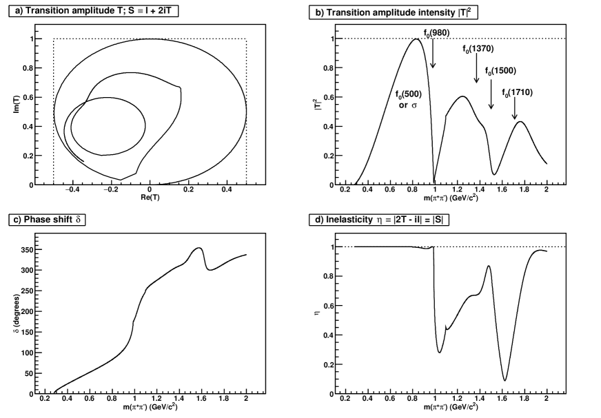
In order to better understand the properties of the $K$-matrix description we will now show a series of instructional plots. The first of these is Fig. 10 which shows the transition amplitude of the $\pi\pi\rightarrow\pi\pi$ S-wave, corresponding to the first element $T_{11}$ of the $T$ matrix defined in Eq. (66), using the parameters given in Table A4 and where we are not considering the effect of the production vector $\hat{P}$. Figure 10a) shows the phase motion of the amplitude, which lies within a circle of unit diameter centred on $(0,i/2$), while Fig. 10b) is the equivalent intensity or amplitude squared. First, we can see that the amplitude follows the unit circle anticlockwise, corresponding to the very broad $\sigma$ or $f_{0}(500)$ resonance structure, until we reach an invariant mass near to the threshold of the $f_{0}(980)$ resonance, where its interference with the $\sigma$ produces a striking dip in the intensity; the amplitude is purely elastic until we reach the $f_{0}(980)$. As we follow the phase motion counterclockwise, new channels such as $K\bar{K}$ open up at higher energies, producing other resonance structures that give extra interference terms and so the scattering process remains inelastic. A more detailed discussion of these features is given in Ref. [123], which has a slightly different amplitude intensity distribution at high invariant mass owing to different scattering data being considered. If we now imagine a vector $\ell$ starting from the centre of the unitarity circle $(0,i/2)$ and ending on the position of the complex amplitude $T_{11}$, then the phase shift $\delta$ is defined as half of the angle that $\ell$ subtends with the imaginary axis (anticlockwise is positive):

$$\delta\equiv\frac{1}{2}{\rm{tan}}^{-1}\left(\frac{{\rm{Im}}T_{11}-\frac{1}{2}}{|{\rm{Re}}T_{11}|}\right)+\frac{\pi}{4}\hskip 14.22636pt\rm{radians},$$ (83)

while the inelasticity $\eta$ is defined as twice the length of $\ell$

$$\eta\equiv 2\left|T_{11}-{\frac{i}{2}}\right|=|S|=2\sqrt{({\rm{Im}}T_{11}-{\scriptstyle{\frac{1}{2}}})^{2}+({\rm{Re}}T_{11})^{2}}.$$ (84)

Figure 10c) shows the evolution of $\delta$ with invariant $\pi\pi$ mass, while Fig. 10d) shows the variation of the inelasticity $\eta$, where a purely elastic (inelastic) process has $\eta=1$ ($\eta=0$); rapid changes in $\delta$ and $\eta$ are observed at the thresholds of various resonance structures.

Figure 11: First row of the $\hat{K}$ matrix, where red (blue) lines show only the pole (SVP) terms, while the black (magenta) lines show the full elements with (without) the Adler zero factor.

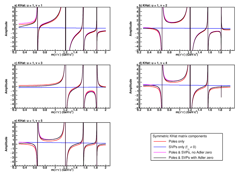
We now move onto the $\hat{K}$ matrix itself, which is the main ingredient of the scattering propagator. Figure 11 shows the first row of the $\hat{K}$ matrix ($\hat{K}_{1j}$), where we have split up the various components that make up each matrix element. The red lines show only the bare pole $m_{\alpha}$ contributions, given by the first summation term on the right hand side of Eq. (71), where $u=1$, $v=1-5$ and we sum over all five poles ($\alpha=1-5$), and the Adler zero suppression factor $f_{A0}(s)$ is set to unity. All of the plots show the strong effect of the bare pole singularities. The blue lines show the rather small SVP contributions, corresponding to the second term on the right hand side of Eq. (71) (with $f_{A0}(s)=1$). The summation of these various pole and SVP contributions is given by the magenta lines, while the black lines show the inclusion of the Adler zero suppression factor of Eq. (72), which only significantly effects the overall shapes at low invariant mass ($m\lesssim 0.5\,{\mathrm{\,Ge\kern-1.00006ptV\!/}c^{2}}$). The absence of singularities for $\hat{K}_{13}$ below $1.2\,{\mathrm{\,Ge\kern-1.00006ptV\!/}c^{2}}$ is due to the fact that the coupling of the first two bare poles in the $4\pi$ channel is zero. Similar distributions are obtained for the other rows of the $\hat{K}$ matrix.

Figure 12: Complex amplitude components of the first row of the propagator $[I-i\hat{K}\rho]^{-1}_{1v}$ ($v\rightarrow\pi\pi$ channels), where red (blue) lines show the real (imaginary) components while the black curves show the magnitudes. The dotted horizontal lines denote the zero amplitude level. Channels are a) $\pi\pi$, b) $K\bar{K}$, c) $4\pi$, d) $\eta\eta$ and e) $\eta\eta^{\prime}$.

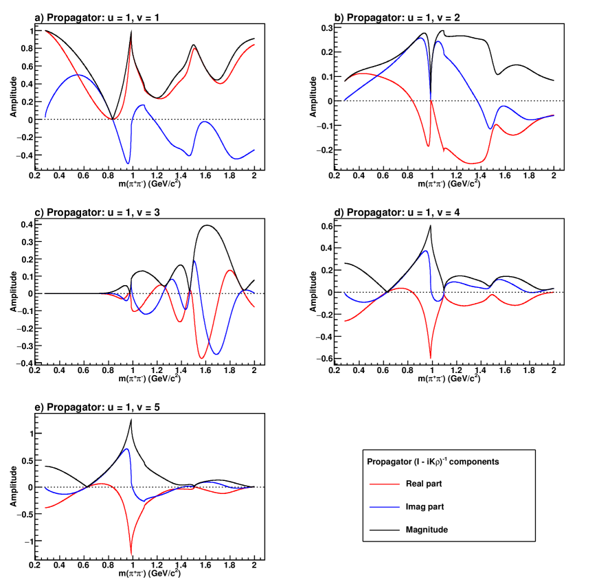
Next, let us look at the $s$-dependence of the first row of the propagator matrix $[I-i\hat{K}\rho]^{-1}_{1v}$, since this will effectively modulate the individual production pole and SVP shapes that are combined to form the total $\pi\pi$ S-wave amplitude ${\cal{F}}_{1}(s)$ using Eq. (70). Figure 12 shows the real and imaginary components, as well as the magnitude, of the propagator elements. The overall impression we get is that the propagator amplitudes have non-trivial variations as a function of $\sqrt{s}$, owing to the matrix inversion process mixing and transposing the superposition of the bare pole states $m_{\alpha}$. These poles essentially produce the various cusps and peaks in the propagator amplitude, where the channel couplings $g_{u,v}^{(\alpha)}$ and phase space $\rho_{u,v}$ (mass threshold) weighting factors shift and distort these features away from the original $m_{\alpha}$ values. The corresponding Argand diagrams show similar behaviour as the transition amplitude $T_{11}$ shown in Fig. 10a), although in general they exhibit distortions due to the channel-dependent couplings and mass thresholds. In particular, the $\pi\pi\rightarrow\pi\pi$ propagator ($u=1,v=1$) exactly matches the phase motion of $T_{11}$ if we first rotate $T_{11}$ by 90 degrees anticlockwise ($\delta$ = 45 degrees) around the centre of the unitarity circle at $(0,\frac{i}{2})$ and then shift it by the translation $(\frac{1}{2},-\frac{i}{2})$.

Discussing the features in Fig. 12 in detail, the first pole ($m_{1}=0.651$ ${\mathrm{\,Ge\kern-1.00006ptV\!/}c^{2}}$) produces the first cusps around 0.65–0.8 ${\mathrm{\,Ge\kern-1.00006ptV\!/}c^{2}}$ in all of the channels, except for $4\pi$ ($v=3$) which has a coupling of zero. The second pole ($m_{2}=1.2036$ ${\mathrm{\,Ge\kern-1.00006ptV\!/}c^{2}}$) produces cusps at 1, 1.1 and 1.5 ${\mathrm{\,Ge\kern-1.00006ptV\!/}c^{2}}$ for the $K\bar{K}$ $(v=2)$, $\eta\eta$ $(v=4)$ and $\eta\eta^{\prime}$ $(v=5)$ channels, respectively, and also generates a very broad dip centred near 1.2 ${\mathrm{\,Ge\kern-1.00006ptV\!/}c^{2}}$ for the $\pi\pi$ $(v=1)$ channel. The third pole ($m_{3}=1.55817$ ${\mathrm{\,Ge\kern-1.00006ptV\!/}c^{2}}$) generates broad peaks near 1.55 ${\mathrm{\,Ge\kern-1.00006ptV\!/}c^{2}}$, where the low mass end terminates in a cusp at the threshold of the given channel, except for the $\eta\eta^{\prime}$ mode where a narrow cusp at 1.5 ${\mathrm{\,Ge\kern-1.00006ptV\!/}c^{2}}$ is generated against a smoothly varying amplitude. The fourth pole ($m_{4}=1.21$ ${\mathrm{\,Ge\kern-1.00006ptV\!/}c^{2}}$) creates structures very similar to the second pole owing to their almost degenerate mass values, with an additional broad peak around 1.1–1.3 ${\mathrm{\,Ge\kern-1.00006ptV\!/}c^{2}}$ present for the $4\pi$ channel, while the fifth pole ($m_{5}=1.82206$ ${\mathrm{\,Ge\kern-1.00006ptV\!/}c^{2}}$) generates the broad peaks near 1.8 ${\mathrm{\,Ge\kern-1.00006ptV\!/}c^{2}}$ for all channels, with additional cusps at 1 ($K\bar{K}$), 1.1 ($\eta\eta$) and 1.5  ${\mathrm{\,Ge\kern-1.00006ptV\!/}c^{2}}$ ($\eta\eta^{\prime}$) that are very similar to those found for the second and fourth poles.

Figure 13: Complex amplitude components for the production poles defined in Eq. (74), where the red (blue) lines show the real (imaginary) parts, while the black lines show the magnitude. The magenta lines show what happens to the magnitude when it is scaled by the Adler zero suppression factor $f_{A0}(s)$. The dotted horizontal lines denote the zero amplitude level.

Figure 13 shows the pole production amplitudes ${\cal{A}}_{\alpha,u=1}(s)$ defined in Eq. (74), which are formed by modulating the pole singularity term $1/(m^{2}_{\alpha}-s)$ with a weighted sum of the $s$-dependent propagator distributions for all channels $v=1$ to $5$ shown in Fig. 12, along with $\beta_{\alpha}\equiv 1$. Concentrating on the magnitudes, we can see that the first pole ($m_{1}=0.651$ ${\mathrm{\,Ge\kern-1.00006ptV\!/}c^{2}}$) has an amplitude that begins rather flat from the $\pi\pi$ threshold until it starts to peak near 1 ${\mathrm{\,Ge\kern-1.00006ptV\!/}c^{2}}$ before rapidly falling at higher invariant mass. Even though the $\pi\pi$ propagator ($\pi\pi\rightarrow\pi\pi$) is slowly decreasing from unity at the $\pi\pi$ threshold down to zero near 0.8 ${\mathrm{\,Ge\kern-1.00006ptV\!/}c^{2}}$, the presence of both the rapid rise of the amplitude from the pole singularity at 0.65 ${\mathrm{\,Ge\kern-1.00006ptV\!/}c^{2}}$ as well as the increasingly influential $K\bar{K}$ propagator ($K\bar{K}\rightarrow\pi\pi$), owing to its larger coupling constant, ensures that the amplitude remains fairly constant in the region below 1 ${\mathrm{\,Ge\kern-1.00006ptV\!/}c^{2}}$. The propagators for all of the channels (except $4\pi$) have a peak near 1 ${\mathrm{\,Ge\kern-1.00006ptV\!/}c^{2}}$, and these combine to give the same local peak for the first production pole. As we increase the invariant mass, the falling shape of the pole singularity starts to dominate the amplitude modulation, and so we get a rapid reduction in the magnitude no matter what shapes the propagators have. The amplitude for the second production pole ($m_{2}=1.2036$ ${\mathrm{\,Ge\kern-1.00006ptV\!/}c^{2}}$) strongly depends upon the $\pi\pi$ and $K\bar{K}$ propagator shapes, where the former has a coupling constant almost double that of the latter. As we decrease the invariant mass from $1.2$ ${\mathrm{\,Ge\kern-1.00006ptV\!/}c^{2}}$, the pole amplitude would be very small at the strong $K\bar{K}$ dip at 1 ${\mathrm{\,Ge\kern-1.00006ptV\!/}c^{2}}$ if not for the compensating sharp peak in the $\pi\pi$ propagator. Likewise, the zero $\pi\pi$ propagator amplitude at 0.8 ${\mathrm{\,Ge\kern-1.00006ptV\!/}c^{2}}$ is nullified by the non-zero $K\bar{K}$ contribution. These two effects conspire to shift the location of the sharp dip in the production pole amplitude by 50 ${\mathrm{\,Me\kern-1.00006ptV\!/}c^{2}}$ from 1 to 0.95 ${\mathrm{\,Ge\kern-1.00006ptV\!/}c^{2}}$. As we decrease the invariant mass, the pole amplitude becomes more influenced by the rising $\pi\pi$ propagator until it starts to fall as we move further away from the pole mass. Above 1.2 ${\mathrm{\,Ge\kern-1.00006ptV\!/}c^{2}}$ the production amplitude tends to follow the undulations of the $\pi\pi$ and $K\bar{K}$ propagators, producing broad local peaks centred on 1.3 and 1.9 ${\mathrm{\,Ge\kern-1.00006ptV\!/}c^{2}}$ as well as a more narrow one at 1.5 ${\mathrm{\,Ge\kern-1.00006ptV\!/}c^{2}}$. The modulation of the third pole ($m_{3}=1.55817$ ${\mathrm{\,Ge\kern-1.00006ptV\!/}c^{2}}$) amplitude is dominated by the $4\pi$ channel, although the other channels give significant contributions, varying from 33% ($\eta\eta$) up to 66% $(\pi\pi$). The $4\pi$ propagator has a very broad maximum centred very close to the pole mass, and so we would expect the production pole peak to remain very close to 1.56 ${\mathrm{\,Ge\kern-1.00006ptV\!/}c^{2}}$ (with an asymmetric width that is slightly narrower on the low side). However, as we decrease the invariant mass, the rising contributions from the $\pi\pi$ and $K\bar{K}$ propagators effectively shift the production peak by 60 ${\mathrm{\,Me\kern-1.00006ptV\!/}c^{2}}$ down to 1.5 ${\mathrm{\,Ge\kern-1.00006ptV\!/}c^{2}}$. Below 1.2 ${\mathrm{\,Ge\kern-1.00006ptV\!/}c^{2}}$, the modulations from the $\pi\pi$ and $K\bar{K}$ propagators become washed out since they are too far away from the pole position. Above 1.5 ${\mathrm{\,Ge\kern-1.00006ptV\!/}c^{2}}$, the width of the production amplitude remains very wide owing to the dominant $4\pi$ propagator. The fourth pole located at 1.21 ${\mathrm{\,Ge\kern-1.00006ptV\!/}c^{2}}$ is almost degenerate with the second pole (1.2036 ${\mathrm{\,Ge\kern-1.00006ptV\!/}c^{2}}$) and so we would naively expect them to have essentially identical production shapes. However, the coupling coefficients are completely different, where now the $4\pi$ channel propagator dominates, with a factor of two or more reduction in the other contributions, leading to the production of the two broad peaks centred around 1.4 and 1.7 ${\mathrm{\,Ge\kern-1.00006ptV\!/}c^{2}}$. For invariant masses at 1 ${\mathrm{\,Ge\kern-1.00006ptV\!/}c^{2}}$ and below, the amplitude does indeed closely follow the shape of the second production pole since the $4\pi$ propagator becomes negligible and the $\pi\pi$ and $K\bar{K}$ contributions dominate. The fifth and last pole ($m_{2}=1.82206$ ${\mathrm{\,Ge\kern-1.00006ptV\!/}c^{2}}$) has an amplitude that is strongly influenced by the $4\pi$ channel, with much smaller contributions from the others. The large, broad $4\pi$ propagator maximum near 1.6 ${\mathrm{\,Ge\kern-1.00006ptV\!/}c^{2}}$ shifts the production peak by around 70 ${\mathrm{\,Me\kern-1.00006ptV\!/}c^{2}}$ down to 1.75 ${\mathrm{\,Ge\kern-1.00006ptV\!/}c^{2}}$, while the other smaller production peaks near 1.4 and 1.1 ${\mathrm{\,Ge\kern-1.00006ptV\!/}c^{2}}$ match those seen in the $4\pi$ shape. The magenta lines in Fig. 13 show the effect of multiplying the Adler zero suppression factor $f_{A0}(s)$ to the production pole amplitudes, where we can see that it only reduces the magnitudes for invariant masses below 1 ${\mathrm{\,Ge\kern-1.00006ptV\!/}c^{2}}$.

The mass distributions of the SVP production amplitudes ${\cal{A}}_{{\rm{SVP}},u=1,v}(s)$ defined in Eq. (75) follows very closely the shape modulations of the propagator terms shown in Fig. 12 (when $f_{v}^{\rm{prod}}\equiv 1$), since each SVP is simply equal to the propagator multiplied by the common function $4/(s+3)$, obtained using $m_{0}^{2}=1.0$ ${\mathrm{\,Ge\kern-1.00006ptV^{2}\!/}c^{4}}$ and $s_{0}^{\rm{prod}}=-3.0$ ${\mathrm{\,Ge\kern-1.00006ptV^{2}\!/}c^{4}}$, which enhances (suppresses) features at low (high) invariant mass.

Figure 14: Mass projections of the individual production pole (left) and SVP (right) amplitudes, with the $\rho(770)$ resonance shown for comparison.

The final set of pedagogical plots are given in Fig. 14, which show the normalised mass projections of the individual production pole and SVP amplitudes, as well as the $\rho(770)$ resonance for comparison, using events generated uniformly across the Dalitz plot. In general, we see that the peaking structures observed in Fig. 13 are replicated here, with a reduction in the intensity as the invariant mass approaches the $\pi\pi$ threshold (fewer events are generated at the kinematic boundary), with an almost flat intensity seen for invariant masses above 2 ${\mathrm{\,Ge\kern-1.00006ptV\!/}c^{2}}$, which is the effective cut-off for the $K$-matrix parameterisation owing to the fact that there are no bare poles defined in this region. The first production pole generates the peak corresponding to the $f_{0}(980)$ along with a broad shoulder on the low mass side, which can be referred to as the $f_{0}(500)$ or $\sigma$ resonance. The third pole generates the $f_{0}(1500)$ peak, the fifth pole is the main contributor for the $f_{0}(1710)$, while a combination of the second and fourth poles (which have almost degenerate bare masses) produces peaks in the $f_{0}(1370)$ region. All of these peaks are generated dynamically by the $K$-matrix amplitude. The first two SVPs have rather oscillatory shapes in the region around 1 to 2 ${\mathrm{\,Ge\kern-1.00006ptV\!/}c^{2}}$; when they are combined we can approximately obtain a very broad bump between the $f_{0}(980)$ and $f_{0}(1370)$ peak locations. The third SVP generates a large peak very near 1.6 ${\mathrm{\,Ge\kern-1.00006ptV\!/}c^{2}}$, in between the $f_{0}(1500)$ and $f_{0}(1710)$ regions. Lastly, the fourth and fifth SVPs are essentially degenerate, peaking at the same position of the $f_{0}(980)$ from the first production pole. This means that we can ignore these two contributions, or at least remove the fifth SVP, since nothing is gained by their inclusion in the total amplitude description.

Appendix B Formulae for available angular distributions

The angular distributions and Blatt–Weisskopf form factors set out in Sec. 2.2 are the default settings in Laura⁺⁺. However, other formalisms to describe the angular distributions are also implemented in the package and it is straightforward to switch between them. This appendix details these alternative formalisms and illustrates the few additional lines of code required to use them.

The four spin-factor formalisms are defined in the enumeration LauAbsResonance::LauSpinType, which can take the values Zemach_P (the default setting), Zemach_Pstar, Covariant, and Legendre. The simplest description of the spin factors is that of the Legendre formalism, where the spin factors are simply the Legendre polynomials (with some additional numerical constants in order to maintain consistency of the phase conventions among the various formalisms)

$$L=0\ :\ T(\vec{p},\vec{q}) = \phantom{-}\,1\,,$$ (85)

$$L=1\ :\ T(\vec{p},\vec{q}) = -\,2\,\cos{\theta}\,,$$ (86)

$$L=2\ :\ T(\vec{p},\vec{q}) = \phantom{-}\,\frac{4}{3}\left[3\cos^{2}{\theta}-1\right]\,,$$ (87)

$$L=3\ :\ T(\vec{p},\vec{q}) = -\,\frac{24}{15}\left[5\cos^{3}{\theta}-3\cos{\theta}\right]\,,$$ (88)

$$L=4\ :\ T(\vec{p},\vec{q}) = \phantom{-}\,\frac{16}{35}\left[35\cos^{4}{\theta}-30\cos^{2}{\theta}+3\right]\,,$$ (89)

$$L=5\ :\ T(\vec{p},\vec{q}) = -\,\frac{32}{63}\left[63\cos^{5}{\theta}-70\cos^{3}{\theta}+15\cos{\theta}\right]\,.$$ (90)

The spin factors for Zemach_P are those given in Eqs. (9)–(14), which differ from the expressions of Eqs. (85)–(90) by factors of $(p\,q)^{L}$. Similarly, those for Zemach_Pstar are the same as those for Zemach_P but with the bachelor momentum evaluated in the rest frame of the parent particle ($p^{\ast}$), rather than that of the resonance ($p$). The angular distributions have been implemented in Laura⁺⁺ up to $L=5$, which is two units larger than the maximum spin of any resonance observed to be produced in any Dalitz plot to date [87, 88, 124].

The angular distributions discussed above are based on a non-relativistic assumption. For certain channels, this may not be sufficiently precise, and therefore the Covariant formalism is also made available. This is given by

$$L=0\ :\ T(\vec{p},\vec{q}) = \phantom{-}\,1\,,$$ (91)

$$L=1\ :\ T(\vec{p},\vec{q}) = -\,2\,(p^{\ast}q)\sqrt{1+\frac{p^{2}}{m^{2}_{P}}}\,\cos{\theta}\,,$$ (92)

$$L=2\ :\ T(\vec{p},\vec{q}) = \phantom{-}\,\frac{4}{3}\,(p^{\ast}q)^{2}\left(\frac{3}{2}+\frac{p^{2}}{m^{2}_{P}}\right)\left[3\cos^{2}{\theta}-1\right]\,,$$ (93)

$$L=3\ :\ T(\vec{p},\vec{q}) = -\,\frac{24}{15}\,(p^{\ast}q)^{3}\sqrt{1+\frac{p^{2}}{m^{2}_{P}}}\left(\frac{5}{2}+\frac{p^{2}}{m^{2}_{P}}\right)\left[5\cos^{3}{\theta}-3\cos{\theta}\right]\,,$$ (94)

$$L=4\ :\ T(\vec{p},\vec{q}) = \phantom{-}\,\frac{16}{35}\,(p^{\ast}q)^{4}\left(\frac{8p^{4}}{m^{4}_{P}}+\frac{40p^{2}}{m^{2}_{P}}+35\right)\left[35\cos^{4}{\theta}-30\cos^{2}{\theta}+3\right]\,.$$ (95)

The first three of these expressions are derived in Ref. [125] and, based on that work, the last two were derived in Ref. [124]. As can be seen from the expressions, the differences between formalisms are more significant for higher spin resonances, and particularly affect tails of the distributions. To give an idea of the effect, the lineshapes for the $f_{2}(1270)$ and $\rho_{3}(1690)^{0}$ resonances decaying to ${{\pi}^{+}}{{\pi}^{-}}$ are shown in Fig. 15.

Figure 15: Lineshapes for the (left) $f_{2}(1270)$ and (right) $\rho_{3}(1690)^{0}$ resonances decaying to ${{\pi}^{+}}{{\pi}^{-}}$ (in the ${{{B}^{+}}}\rightarrow{{K}^{+}}{{\pi}^{+}}{{\pi}^{-}}$ Dalitz plot) with the (blue) Legendre, (red) Zemach_P, (green) Zemach_Pstar and (magenta) Covariant spin formalisms. In all cases the relativistic Breit–Wigner description is used, with mass and width parameters as given in App. C and the two Blatt–Weisskopf factors set to unity.

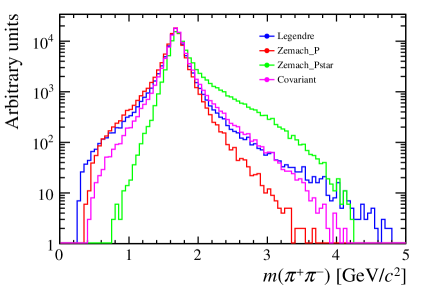
It is possible to switch between these different formalisms via a function of the LauResonanceMaker factory object. For example, to use the Covariant formalism one would do:

⬇

LauResonanceMaker& resMaker = LauResonanceMaker::get();

resMaker.setSpinFormalism( LauAbsResonance::Covariant );

It is important to note that any such operation must be performed prior to constructing any resonances, i.e. before calling LauIsobarDynamics::addResonance or LauIsobarDynamics::addIncoherentResonance for the first time.

As the angular and Blatt–Weisskopf factors are strongly coupled, it is also possible to straightforwardly modify the form of the Blatt–Weisskopf factors. In particular, the momentum value used for the factor that is related to the decay of the parent particle into the resonance and the bachelor can be selected from the following options (defined in the LauBlattWeisskopfFactor::RestFrame enumeration):

• LauBlattWeisskopfFactor::ResonanceFrame, the momentum of the bachelor in the rest frame of the resonance, $p$ (the default setting),

• LauBlattWeisskopfFactor::ParentFrame, the momentum of the bachelor in the rest frame of the parent, $p^{\ast}$,

• LauBlattWeisskopfFactor::Covariant, the product of the momentum of the bachelor in the rest frame of the parent, $p^{\ast}$, and a function of the ratio of the energy and mass of the resonance in the rest frame of the parent, $\sqrt{1+p^{2}/m^{2}_{P}}$. More precisely, this function is the expression in the middle term in Eqs. (91) to (95) raised to the power of $1/L$.

This setting is changed as follows:

⬇

LauResonanceMaker& resMaker = LauResonanceMaker::get();

resMaker.setBWBachelorRestFrame( LauBlattWeisskopfFactor::ParentFrame );

where in this example the momentum of the bachelor in the rest frame of the parent ($p^{\ast}$) is to be used. Again, this operation must be performed before constructing any resonances.

In addition, it is possible to change the form of the Blatt–Weisskopf factors, with the different types being defined by the LauBlattWeisskopfFactor::BarrierType enumeration. The default setting, corresponding to Eqs. (15)–(20), is given by LauBlattWeisskopfFactor::BWPrimeBarrier and is recommended when the angular terms contain momentum factors. One possible alternative is to use the LauAbsResonance::Legendre angular terms and the LauBlattWeisskopfFactor::BWBarrier form for the Blatt–Weisskopf factors:

$$L=0\ :\ X(z) = 1\,,$$ (96)

$$L=1\ :\ X(z) = \sqrt{\frac{2z^{2}}{1+z^{2}}}\,,$$ (97)

$$L=2\ :\ X(z) = \sqrt{\frac{13z^{4}}{z^{4}+3z^{2}+9}}\,,$$ (98)

$$L=3\ :\ X(z) = \sqrt{\frac{277z^{6}}{z^{6}+6z^{4}+45z^{2}+225}}\,,$$ (99)

$$L=4\ :\ X(z) = \sqrt{\frac{12746z^{8}}{z^{8}+10z^{6}+135z^{4}+1575z^{2}+11025}}\,,$$ (100)

$$L=5\ :\ X(z) = \sqrt{\frac{998881z^{10}}{z^{10}+15z^{8}+315z^{6}+6300z^{4}+99225z^{2}+893025}}\,.$$ (101)

An exponential form for these factors, LauBlattWeisskopfFactor::ExpBarrier, which has been used in some analyses for virtual contributions has also been implemented,

$$X(z)=e^{-z^{L}}\,.$$ (102)

To change the form of the barrier factors for all resonances, the following lines are required

⬇

LauResonanceMaker& resMaker = LauResonanceMaker::get();

resMaker.setBWType( LauBlattWeisskopfFactor::BWBarrier );

where in this example the forms in Eqs. (96)–(101) are to be used. Again, this operation should be performed before constructing any resonances.

As for the $T(\vec{p},\vec{q})$ terms, the differences between Blatt–Weisskopf form factor formalisms are more significant for higher spin resonances, and far from the peak of the resonance. An illustrative comparison of the shapes is given in Fig. 16.

Figure 16: Lineshapes for the (left) $f_{2}(1270)$ and (right) $\rho_{3}(1690)^{0}$ resonances decaying to ${{\pi}^{+}}{{\pi}^{-}}$ (in the ${{{B}^{+}}}\rightarrow{{K}^{+}}{{\pi}^{+}}{{\pi}^{-}}$ Dalitz plot) with (blue) no Blatt–Weisskopf factors, and with the (red) ResonanceFrame, (green) ParentFrame and (magenta) Covariant settings for evaluating the momentum that enters the Blatt–Weisskopf factor associated with the decay of the parent particle. In all cases the relativistic Breit–Wigner description is used, with mass and width parameters as given in App. C and the Zemach_P formalism for the spin factors.

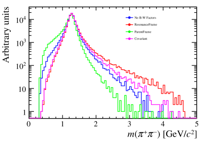
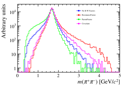
It is possible to make all of the changes discussed in this Appendix at the level of individual resonances, using the functions LauAbsResonance::setSpinType and LauAbsResonance::setBarrierRadii, but this requires much care to be taken and is not generally recommended.

Appendix C Standard resonances

This section provides the complete set of available resonances, indicating the name, mass $m_{0}$, width $\Gamma_{0}$, spin, charge and Blatt–Weisskopf barrier radius $r^{R}_{\rm BW}$. Table C1 contains information for light meson resonances, Table C2 for charm, charmonium, strange-charm, beauty and strange-beauty resonances, Table C3 for $K^{*}$ resonances and Table C4 for nonresonant terms. Most data are taken from Ref. [62]. The tables list the information contained in the information records for both neutral and positively-charged resonances. Negatively-charged resonance records are implemented as charge-conjugates of the positively charged ones; the plus sign in the name is replaced with a minus sign.

In case a user wishes to modify the values of the parameters from those given in the tables, the LauAbsResonance::changeResonance function, which takes the mass, width and spin as arguments, can be used. The Blatt–Weisskopf barrier radius can be changed with the LauAbsResonance::changeBWBarrierRadii function, and other parameters specific to particular lineshapes can be changed with the LauAbsResonance::setResonanceParameter function. The same approach can be used to include a resonance that is not available in these tables, by using any of the existing states of appropriate charge and redefining its properties.

Table C1: Standard light meson resonances defined in Laura⁺⁺.

Name	$m_{0}$ (${\mathrm{Ge\kern-1.00006ptV\!/}c^{2}}$)	$\Gamma_{0}$ (${\mathrm{Ge\kern-1.00006ptV\!/}c^{2}}$)	spin	charge	$r^{R}_{\rm BW}$ ($\mathrm{Ge\kern-1.00006ptV}^{-1}$)
rho0(770)	0.77526	0.1478	1	0	5.3
rho+(770)	0.77511	0.1491	1	1	5.3
rho0(1450)	1.465	0.400	1	0	4.0
rho+(1450)	1.465	0.400	1	1	4.0
rho0(1700)	1.720	0.250	1	0	4.0
rho+(1700)	1.720	0.250	1	1	4.0
rho0(1900)	1.909	0.130	1	0	4.0
rho+(1900)	1.909	0.130	1	1	4.0
rho0_3(1690)	1.686	0.186	3	0	4.0
rho+_3(1690)	1.686	0.186	3	1	4.0
rho0_3(1990)	1.982	0.188	3	0	4.0
rho+_3(1990)	1.982	0.188	3	1	4.0
phi(1020)	1.019461	0.004266	1	0	4.0
phi(1680)	1.680	0.150	1	0	4.0
f_0(980)	0.990	0.070	0	0	—
f_2(1270)	1.2751	0.1851	2	0	4.0
f_0(1370)	1.370	0.350	0	0	—
f’_0(1300)	1.449	0.126	0	0	—
f_2(1430)	1.430	0.150	2	0	4.0
f_0(1500)	1.505	0.109	0	0	—
f’_2(1525)	1.525	0.073	2	0	4.0
f_2(1565)	1.562	0.134	2	0	4.0
f_2(1640)	1.639	0.099	2	0	4.0
f_0(1710)	1.722	0.135	0	0	—
f_2(1810)	1.816	0.197	2	0	4.0
f_2(1910)	1.903	0.196	2	0	4.0
f_2(1950)	1.944	0.472	2	0	4.0
f_2(2010)	2.011	0.202	2	0	4.0
f_0(2020)	1.992	0.442	0	0	—
f_4(2050)	2.018	0.237	4	0	4.0
f_0(2100)	2.101	0.224	0	0	—
omega(782)	0.78265	0.00849	1	0	4.0
a0_0(980)	0.980	0.092	0	0	—
a+_0(980)	0.980	0.092	0	1	—
a0_0(1450)	1.474	0.265	0	0	—
a+_0(1450)	1.474	0.265	0	1	—
a0_2(1320)	1.3190	0.1050	2	0	4.0
a+_2(1320)	1.3190	0.1050	2	1	4.0
sigma0	0.475	0.550	0	0	—
sigma+	0.475	0.550	0	1	—

Table C2: Standard charm, charmonium, strange-charm, beauty and strange-beauty resonances defined in Laura⁺⁺.

Name	$m_{0}$ (${\mathrm{Ge\kern-1.00006ptV\!/}c^{2}}$)	$\Gamma_{0}$ (${\mathrm{Ge\kern-1.00006ptV\!/}c^{2}}$)	spin	charge	$r^{R}_{\rm BW}$ ($\mathrm{Ge\kern-1.00006ptV}^{-1}$)
chi_c0	3.41475	0.0105	0	0	—
chi_c1	3.51066	0.00084	1	0	4.0
chi_c2	3.55620	0.00193	2	0	4.0
X(3872)	3.87169	0.0012	1	0	4.0
dabba0	2.098	0.520	0	0	—
dabba+	2.098	0.520	0	1	—
D*0	2.00696	0.0021	1	0	4.0
D*+	2.01026	$83.4\times 10^{-6}$	1	1	4.0
D*0_0	2.318	0.267	0	0	—
D*+_0	2.403	0.283	0	1	—
D*0_2	2.4626	0.049	2	0	4.0
D*+_2	2.4643	0.037	2	1	4.0
D0_1(2420)	2.4214	0.0274	1	0	4.0
D+_1(2420)	2.4232	0.025	1	1	4.0
D0(2600)	2.612	0.093	0	0	—
D+(2600)	2.612	0.093	0	1	—
D0(2760)	2.761	0.063	1	0	4.0
D+(2760)	2.761	0.063	1	1	4.0
D0(3000)	3.0	0.15	0	0	—
D0(3400)	3.4	0.15	0	0	—
Ds*+	2.1121	0.0019	1	1	4.0
Ds*+_0(2317)	2.3177	0.0038	0	1	—
Ds*+_2(2573)	2.5719	0.017	2	1	4.0
Ds*+_1(2700)	2.709	0.117	1	1	4.0
Ds*+_1(2860)	2.862	0.180	1	1	4.0
Ds*+_3(2860)	2.862	0.058	3	1	4.0
B*0	5.3252	0.00	1	0	6.0
B*+	5.3252	0.00	1	1	6.0
Bs*0	5.4154	0.00	1	0	6.0

Table C3: Standard $K^{*}$ resonances defined in Laura⁺⁺.

Name	$m_{0}$ (${\mathrm{Ge\kern-1.00006ptV\!/}c^{2}}$)	$\Gamma_{0}$ (${\mathrm{Ge\kern-1.00006ptV\!/}c^{2}}$)	spin	charge	$r^{R}_{\rm BW}$ ($\mathrm{Ge\kern-1.00006ptV}^{-1}$)
K*0(892)	0.89581	0.0474	1	0	3.0
K*+(892)	0.89166	0.0508	1	1	3.0
K*0(1410)	1.414	0.232	1	0	4.0
K*+(1410)	1.414	0.232	1	1	4.0
K*0_0(1430)	1.425	0.270	0	0	—
K*+_0(1430)	1.425	0.270	0	1	—
K*0_2(1430)	1.4324	0.109	2	0	4.0
K*+_2(1430)	1.4256	0.0985	2	1	4.0
K*0(1680)	1.717	0.322	1	0	4.0
K*+(1680)	1.717	0.322	1	1	4.0
K*0_0(1950)	1.945	0.201	0	0	—
K*+_0(1950)	1.945	0.201	0	1	—
kappa0	0.682	0.547	0	0	—
kappa+	0.682	0.547	0	1	—

Table C4: Standard nonresonant terms defined in Laura⁺⁺.

Name	$m_{0}$ (${\mathrm{Ge\kern-1.00006ptV\!/}c^{2}}$)	$\Gamma_{0}$ (${\mathrm{Ge\kern-1.00006ptV\!/}c^{2}}$)	spin	charge
NonReson	0.0	0.0	0	0
NRModel	0.0	0.0	0	0
BelleSymNR	0.0	0.0	0	0
BelleNR	0.0	0.0	0	0
BelleNR+	0.0	0.0	0	1
BelleNR_Swave	0.0	0.0	0	0
BelleNR_Swave+	0.0	0.0	0	1
BelleNR_Pwave	0.0	0.0	1	0
BelleNR_Pwave+	0.0	0.0	1	1
BelleNR_Dwave	0.0	0.0	2	0
BelleNR_Dwave+	0.0	0.0	2	1
BelleNR_Fwave	0.0	0.0	3	0
BelleNR_Fwave+	0.0	0.0	3	1
NRTaylor	0.0	0.0	0	0
PolNR_S0	0.0	0.0	0	0
PolNR_S1	0.0	0.0	0	0
PolNR_S2	0.0	0.0	0	0
PolNR_P0	0.0	0.0	1	0
PolNR_P1	0.0	0.0	1	0
PolNR_P2	0.0	0.0	1	0

Appendix D PDF classes

This section details the formulae within classes that can be used to parameterise additional PDFs ${\cal P}(x;p_{1},p_{2},...,p_{n})$ for the likelihood function. Here, $x$ denotes the dependent variable, while $p_{1},p_{2},...,p_{n}$ is the list of parameters in the form of a vector of LauParameter objects, each containing a descriptive name (which must contain the case-sensitive word shown in quotes), the value of the parameter and optionally its validity range, uncertainty and constantness. All PDFs used in Laura⁺⁺ are normalised to unity, although the normalisation factors are omitted in many equations in this section for brevity.

D.1 LauArgusPdf

The ARGUS threshold function [126] can be used to parameterise the shape of combinatorial or partially-reconstructed backgrounds of the invariant mass $m$ of parent candidates:

$${\cal P}(x;m_{0},\xi)=x\sqrt{1-x^{2}}e^{-\xi(1-x^{2})}\theta(x)\,,$$ (103)

where $x=m/m_{0}$, $m_{0}$ is the end-point of the curve (“m0”), $\xi$ is the shape parameter (“xi”), while $\theta(x\leq m_{0})=1$ and $\theta(x>m_{0})=0$.

D.2 LauBifurcatedGaussPdf

This PDF is the bifurcation of two Gaussians having different widths, $\sigma_{L}$ (“sigmaL”) or $\sigma_{R}$ (“sigmaR”), to the left or right of the “mean” $\mu$:

$${\cal P}(x;\mu,\sigma_{L},\sigma_{R})=\begin{cases}e^{-(x-\mu)^{2}/(2\sigma_{L}^{2})}&\text{for }x\leq\mu\\ e^{-(x-\mu)^{2}/(2\sigma_{R}^{2})}&\text{for }x>\mu\,.\end{cases}$$ (104)

D.3 LauChebychevPdf

This class implements a sum of Chebyshev polynomials of the first kind $T_{i}$ (up to seventh order):

$${\cal P}(x;c_{i})=1+\sum_{i=1}^{n\leq 7}c_{i}T_{i}(x)\,,$$ (105)

where $c_{i}$ is the parameter coefficient (“c1”, “c2”, etc.) and

$$T_{n}(y)=\frac{(y-\sqrt{y^{2}-1})^{n}+(y+\sqrt{y^{2}-1})^{n}}{2}\,,\hskip 14.22636pty\equiv-1+\frac{2(x-x_{\rm{min}})}{(x_{\rm{max}}-x_{\rm{min}})}\,.$$ (106)

D.4 LauCruijffPdf

The Cruijff PDF is a bifurcated Gaussian, which has different widths $\sigma_{L}$ (“sigmaL”) and $\sigma_{R}$ (“sigmaR”) to the left and right of the “mean” $\mu$, along with asymmetric tails $\alpha_{L}$ (“alphaL”) and $\alpha_{R}$ (“alphaR”):

$${\cal P}(x;\mu,\sigma_{L},\sigma_{R},\alpha_{L},\alpha_{R})=\begin{cases}e^{-(x-\mu)^{2}/(2\sigma_{L}^{2}+\alpha_{L}(x-\mu)^{2})}&\text{for }x\leq\mu\\ e^{-(x-\mu)^{2}/(2\sigma_{R}^{2}+\alpha_{R}(x-\mu)^{2})}&\text{for }x>\mu\,.\end{cases}$$ (107)

D.5 LauCrystalBallPdf

The Crystal Ball function [127] is a PDF that contains a Gaussian core with a continuous power-law tail on one side:

$${\cal P}(x;\mu,\sigma,\alpha,n)=\begin{cases}e^{-\frac{1}{2}t^{2}}&\text{for }t\geq|\alpha|\\ \left(\frac{n}{|\alpha|}\right)^{n}e^{-\frac{1}{2}|\alpha|^{2}}\left(\frac{n}{|\alpha|}-|\alpha|-t\right)^{-n}&\text{otherwise}\,,\end{cases}$$ (108)

where $\mu$ and $\sigma$ are the Gaussian “mean” and width (“sigma”), respectively, $\alpha$ (“alpha”) is the positive or negative distance from the mean in which the Gaussian and the tail parts match up, $n$ (“order”) is the power exponent for the tail, while $t$ is equal to $(x-\mu)/\sigma$, which changes sign if $\alpha$ is negative.

D.6 LauExponentialPdf

This exponential function is simply given by

$${\cal P}(x;\lambda)=e^{\lambda x}\,,$$ (109)

where $\lambda$ is the “slope” parameter.

D.7 LauGaussPdf

The Gaussian PDF is defined by a “mean” $\mu$ and width $\sigma$ (“sigma”):

$${\cal P}(x;\mu,\sigma)=\frac{1}{\sigma\sqrt{2\pi}}e^{-(x-\mu)^{2}/(2\sigma^{2})}\,.$$ (110)

D.8 LauLinearPdf

This linear function only needs the gradient (“slope”) $\lambda$:

$${\cal P}(x;\lambda)=\lambda x+c\,,$$ (111)

where $c$ is the intercept and is evaluated using the range of the abscissa $x$.

D.9 LauNovosibirskPdf

The Novosibirsk PDF is a Gaussian with a logarithmic exponent [128]:

$${\cal P}(x;\mu,\sigma,\tau)=\text{exp}\left[-\frac{1}{2}\left(\frac{\text{ln}^{2}[1+\Lambda\tau(x-\mu)]}{\tau^{2}}+\tau^{2}\right)\right]\,,\hskip 7.11317pt\text{with }\Lambda\equiv\frac{\text{sinh }(\tau\sqrt{\text{ln }4})}{\sigma\tau\sqrt{\text{ln }4}}\,,$$ (112)

where $\mu$ and $\sigma$ are the usual “mean” and width (“sigma”) values, respectively, and $\tau$ is the “tail” parameter; as $\tau\rightarrow 0$, the PDF converges to a normal Gaussian with width $\sigma$.

D.10 LauParametricStepFuncPdf

This parametric step function is a binned distribution whose parameters are the contents of each bin (except one), essentially representing a histogram with variable bin content. The content of the remaining bin is determined from that of the others and the requirement of normalisation. The constructor requires two vectors of LauParameter objects; the first stores the bin contents or weights (which are parameters that can be fitted), while the second stores the lower edge abscissa limits of each bin (in ascending order) as well as the upper edge limit of the last bin. It can also be specified whether the normalisation bin is the first or last; it is advisable to use the bin with the larger content.

D.11 LauSigmoidPdf

The sigmoid function follows an “S” shape and is defined as

$${\cal P}(x;a,b)=\frac{1}{1+e^{b-ax}}\,,$$ (113)

with parameters “a” and “b” defining the steepness of the slope and the shift of the distribution, respectively. A negative value of $a$ will flip the distribution around the ordinate axis.

D.12 LauSumPdf

This class implements the summation of two PDFs, ${\cal P}_{1}$ and ${\cal P}_{2}$, with a relative fraction (“frac”) $f$:

$${\cal P}(x)=f{\cal P}_{1}(x)+(1-f){\cal P}_{2}(x)\,.$$ (114)

D.13 Dalitz-plot-dependent PDFs

What follows are descriptions of PDFs with parameters that can vary across the Dalitz plot via power-law scaling with Laurent polynomials containing either positive or negative exponents. Here, the parameterisation of a given PDF parameter $g$ is given by

$$g=\sum_{i=1}^{n}{c_{i}D^{i}}\hskip 28.45274pt\text{or }\hskip 28.45274ptg=\sum_{i=1}^{n}{c_{i}D^{-i}}\,,$$ (115)

where $D$ is the invariant mass-squared variable representing the DP position and $c_{i}$ is the coefficient of expansion for the power term $i$. The variable $D$ can be either $m^{2}_{13}$, $m^{2}_{23}$, or $m^{2}_{12}$, the minimum or maximum values of $m^{2}_{13}$ or $m^{2}_{23}$, or the distance from the DP centre. The constructors of these PDFs require vectors of the coefficients $c_{i}$ for each function parameter $g$, as well as the pointer to the LauDaughters object in order to find $D$ from the kinematics. The LauDPDepBifurGaussPdf, LauDPDepCruijffPdf and LauDPDepGaussPdf classes represent bifurcated Gaussian, Cruijff and normal Gaussian PDFs, given in Eqs. (104), (107) and (110) respectively, with parameters that can vary according to Eq. (115).

The LauDPDepMapPdf class can be used to define a PDF that requires different functions depending on the DP region. It uses a Root histogram that divides the DP, or its projection onto one axis, into ascending, numbered regions. The region number (starting from zero) for a given value of $D$ is then used to choose the corresponding PDF from the ordered list of functions provided as a vector in the constructor.

The LauDPDepSumPdf class implements the sum of two PDFs, defined by Eq. (114), in which the fraction $f$ (“frac”) depends on the variable $D$, using either the contents from a two-dimensional histogram directly or a vector of coefficients $c_{i}$ for the positive-power Laurent polynomial shown in Eq. (115).

References

- [1] R. H. Dalitz, On the analysis of tau-meson data and the nature of the tau-meson, Phil. Mag. 44 (1953) 1068
- [2] E. Fabri, A study of tau-meson decay, Nuovo Cim. 11 (1954) 479
- [3] Crystal Barrel collaboration, C. Amsler et al., Coupled channel analysis of annihilation into , and , Phys. Lett. B355 (1995) 425
- [4] BaBar collaboration, J. P. Lees et al., Dalitz plot analysis of and in two-photon interactions, Phys. Rev. D89 (2014) 112004, arXiv:1403.7051
- [5] BaBar collaboration, J. P. Lees et al., Measurement of the I=1/2 -wave amplitude from Dalitz plot analyses of in two-photon interactions, Phys. Rev. D93 (2016) 012005, arXiv:1511.02310
- [6] N. Cabibbo, Unitary symmetry and leptonic decays, Phys. Rev. Lett. 10 (1963) 531
- [7] M. Kobayashi and T. Maskawa, violation in the renormalizable theory of weak interaction, Prog. Theor. Phys. 49 (1973) 652
- [8] R. H. Schindler et al., Measurements of the properties of meson decays, Phys. Rev. D24 (1981) 78
- [9] MARK III collaboration, J. Adler et al., Resonant substructure in decays of charmed mesons, Phys. Lett. B196 (1987) 107
- [10] E691 collaboration, J. C. Anjos et al., A Dalitz plot analysis of decays, Phys. Rev. D48 (1993) 56
- [11] ARGUS collaboration, H. Albrecht et al., A partial wave analysis of the decay , Phys. Lett. B308 (1993) 435
- [12] E687 collaboration, P. L. Frabetti et al., Analysis of three Dalitz plots, Phys. Lett. B331 (1994) 217
- [13] CLEO collaboration, S. Kopp et al., Dalitz analysis of the decay , Phys. Rev. D63 (2001) 092001, arXiv:hep-ex/0011065
- [14] E791 collaboration, E. M. Aitala et al., Model independent measurement of S-wave systems using decays from Fermilab E791, Phys. Rev. D73 (2006) 032004, erratum ibid. D74 (2006) 059901, arXiv:hep-ex/0507099
- [15] CLEO collaboration, G. Bonvicini et al., Dalitz plot analysis of the decay, Phys. Rev. D78 (2008) 052001, arXiv:0802.4214
- [16] FOCUS collaboration, J. M. Link et al., The S-wave from the decay, Phys. Lett. B681 (2009) 14, arXiv:0905.4846
- [17] BaBar collaboration, P. del Amo Sanchez et al., Analysis of the decay channel, Phys. Rev. D83 (2011) 072001, arXiv:1012.1810
- [18] BaBar collaboration, B. Aubert et al., Amplitude analysis of the decay , Phys. Rev. D76 (2007) 011102, arXiv:0704.3593
- [19] BaBar collaboration, B. Aubert et al., Dalitz plot analysis of , Phys. Rev. D79 (2009) 032003, arXiv:0808.0971
- [20] E791 collaboration, E. M. Aitala et al., Experimental evidence for a light and broad scalar resonance in decay, Phys. Rev. Lett. 86 (2001) 770, arXiv:hep-ex/0007028
- [21] CLEO collaboration, H. Muramatsu et al., Dalitz analysis of , Phys. Rev. Lett. 89 (2002) 251802, erratum ibid. 90 (2003) 059901, arXiv:hep-ex/0207067
- [22] FOCUS collaboration, J. M. Link et al., Dalitz plot analysis of and decay to using the K-matrix formalism, Phys. Lett. B585 (2004) 200, arXiv:hep-ex/0312040
- [23] CLEO collaboration, G. Bonvicini et al., Dalitz plot analysis of the decay, Phys. Rev. D76 (2007) 012001, arXiv:0704.3954
- [24] J. R. Pelaez, From controversy to precision on the sigma meson: a review on the status of the non-ordinary resonance, Phys. Rept. 658 (2016) 1, arXiv:1510.00653
- [25] BaBar collaboration, B. Aubert et al., The BaBar detector, Nucl. Instrum. Meth. A479 (2002) 1, arXiv:hep-ex/0105044
- [26] BaBar collaboration, B. Aubert et al., The BaBar detector: Upgrades, operation and performance, Nucl. Instrum. Meth. A729 (2013) 615, arXiv:1305.3560
- [27] Belle collaboration, A. Abashian et al., The Belle detector, Nucl. Instrum. Meth. A479 (2002) 117
- [28] Belle collaboration, K. Abe et al., Study of decays, Phys. Rev. D69 (2004) 112002, arXiv:hep-ex/0307021
- [29] BaBar collaboration, B. Aubert et al., Dalitz plot analysis of , Phys. Rev. D79 (2009) 112004, arXiv:0901.1291
- [30] Belle collaboration, A. Kuzmin et al., Study of decays, Phys. Rev. D76 (2007) 012006, arXiv:hep-ex/0611054
- [31] BaBar collaboration, P. del Amo Sanchez et al., Dalitz-plot analysis of , arXiv:1007.4464
- [32] Belle collaboration, A. Garmash et al., Dalitz analysis of the three-body charmless decays and , Phys. Rev. D71 (2005) 092003, arXiv:hep-ex/0412066
- [33] BaBar collaboration, B. Aubert et al., An amplitude analysis of the decay , Phys. Rev. D72 (2005) 052002, arXiv:hep-ex/0507025
- [34] BaBar collaboration, B. Aubert et al., Dalitz-plot analysis of the decays , Phys. Rev. D72 (2005) 072003, erratum ibid. D74 (2006) 099903, arXiv:hep-ex/0507004
- [35] Belle collaboration, A. Garmash et al., Evidence for large direct violation in from analysis of the three-body charmless decay, Phys. Rev. Lett. 96 (2006) 251803, arXiv:hep-ex/0512066
- [36] BaBar collaboration, B. Aubert et al., Evidence for direct violation from Dalitz-plot analysis of , Phys. Rev. D78 (2008) 012004, arXiv:0803.4451
- [37] CLEO collaboration, D. M. Asner et al., Search for – mixing in the Dalitz plot analysis of , Phys. Rev. D72 (2005) 012001, arXiv:hep-ex/0503045
- [38] Belle collaboration, L. M. Zhang et al., Measurement of – mixing parameters in decays, Phys. Rev. Lett. 99 (2007) 131803, arXiv:0704.1000
- [39] BaBar collaboration, B. Aubert et al., Measurement of -violating asymmetries in using a time-dependent Dalitz plot analysis, Phys. Rev. D76 (2007) 012004, arXiv:hep-ex/0703008
- [40] Belle collaboration, A. Kusaka et al., Measurement of asymmetry in a time-dependent Dalitz analysis of and a constraint on the CKM angle , Phys. Rev. Lett. 98 (2007) 221602, arXiv:hep-ex/0701015
- [41] Belle collaboration, A. Kusaka et al., Measurement of asymmetries and branching fractions in a time-dependent Dalitz analysis of and a constraint on the quark mixing angle , Phys. Rev. D77 (2008) 072001, arXiv:0710.4974
- [42] BaBar collaboration, B. Aubert et al., Measurements of -violating asymmetries in the decay , Phys. Rev. Lett. 99 (2007) 161802, arXiv:0706.3885
- [43] Belle collaboration, J. Dalseno et al., Time-dependent Dalitz plot measurement of parameters in decays, Phys. Rev. D79 (2009) 072004, arXiv:0811.3665
- [44] BaBar collaboration, B. Aubert et al., Time-dependent amplitude analysis of , Phys. Rev. D80 (2009) 112001, arXiv:0905.3615
- [45] Belle collaboration, Y. Nakahama et al., Measurement of violating asymmetries in decays with a time-dependent Dalitz approach, Phys. Rev. D82 (2010) 073011, arXiv:1007.3848
- [46] BaBar collaboration, J. P. Lees et al., Measurement of -violating asymmetries in decays using a time-dependent Dalitz plot analysis, Phys. Rev. D88 (2013) 012003, arXiv:1304.3503
- [47] LHCb collaboration, A. A. Alves Jr. et al., The LHCb detector at the LHC, JINST 3 (2008) S08005
- [48] A. E. Snyder and H. R. Quinn, Measuring asymmetry in decays without ambiguities, Phys. Rev. D48 (1993) 2139
- [49] J. Charles et al., time-dependent Dalitz plots, violating angles , , and discrete ambiguities, Phys. Lett. B425 (1998) 375, arXiv:hep-ph/9801363
- [50] T. Latham and T. Gershon, A method to measure using time-dependent Dalitz plot analysis of , J. Phys. G36 (2009) 025006, arXiv:0809.0872
- [51] T. Gershon, On the measurement of the Unitarity Triangle angle from decays, Phys. Rev. D79 (2009) 051301, arXiv:0810.2706
- [52] T. Gershon and M. Williams, Prospects for the measurement of the Unitarity Triangle angle from decays, Phys. Rev. D80 (2009) 092002, arXiv:0909.1495
- [53] R. Brun and F. Rademakers, ROOT: An object oriented data analysis framework, Nucl. Instrum. Meth. A389 (1997) 81
- [54] F. James and M. Roos, Minuit: A system for function minimization and analysis of the parameter errors and correlations, Comput. Phys. Commun. 10 (1975) 343
- [55] Apache License, Version 2.0, 2004. http://www.apache.org/licenses/LICENSE-2.0
- [56] G. N. Fleming, Recoupling effects in the isobar model. 1. General formalism for three-pion scattering, Phys. Rev. 135 (1964) B551
- [57] D. Morgan, Phenomenological analysis of single-pion production processes in the energy range 500 to 700 MeV, Phys. Rev. 166 (1968) 1731
- [58] D. Herndon, P. Soding, and R. J. Cashmore, A generalised isobar model formalism, Phys. Rev. D11 (1975) 3165
- [59] C. Zemach, Three pion decays of unstable particles, Phys. Rev. 133 (1964) B1201
- [60] C. Zemach, Use of angular-momentum tensors, Phys. Rev. 140 (1965) B97
- [61] J. Blatt and V. E. Weisskopf, Theoretical nuclear physics, J. Wiley (New York), 1952
- [62] Particle Data Group, C. Patrignani et al., Review of particle physics, Chin. Phys. C40 (2016) 100001
- [63] W. H. Press, B. P. Flannery, S. A. Teukolsky, and W. T. Vetterling, Numerical recipes in C: The art of scientific computing, Cambridge University Press, 2 ed., 1992
- [64] M. Pivk and F. R. Le Diberder, sPlot: A statistical tool to unfold data distributions, Nucl. Instrum. Meth. A555 (2005) 356, arXiv:physics/0402083
- [65] B. Efron and R. J. Tibshirani, An introduction to the bootstrap, Chapman and Hall, 1993
- [66] R. Barlow, Application of the bootstrap resampling technique to particle physics experiments, http://www.hep.manchester.ac.uk/preprints/manhep99-4.ps, 1999
- [67] P. F. Harrison, Blind analysis, J. Phys. G28 (2002) 2679
- [68] J. R. Klein and A. Roodman, Blind analysis in nuclear and particle physics, Ann. Rev. Nucl. Part. Sci. 55 (2005) 141
- [69] Y. Xie, sFit: a method for background subtraction in maximum likelihood fit, arXiv:0905.0724
- [70] LHCb collaboration, R. Aaij et al., Constraints on the unitarity triangle angle from Dalitz plot analysis of decays, Phys. Rev. D93 (2016) 112018, erratum ibid. D94 (2016) 079902, arXiv:1602.03455
- [71] E. Ben-Haim, R. Brun, B. Echenard, and T. E. Latham, JFIT: a framework to obtain combined experimental results through joint fits, arXiv:1409.5080
- [72] M. Williams, How good are your fits? Unbinned multivariate goodness-of-fit tests in high energy physics, JINST 5 (2010) P09004, arXiv:1006.3019
- [73] BaBar collaboration, B. Aubert et al., Observation of the decay , Phys. Rev. Lett. 99 (2007) 221801, arXiv:0708.0376
- [74] BaBar collaboration, B. Aubert et al., Search for the highly suppressed decays and , Phys. Rev. D78 (2008) 091102, arXiv:0808.0900
- [75] BaBar collaboration, B. Aubert et al., Search for the decay , Phys. Rev. D79 (2009) 051101, arXiv:0811.1979
- [76] BaBar collaboration, P. del Amo Sanchez et al., Observation of the rare decay , Phys. Rev. D82 (2010) 031101, arXiv:1003.0640
- [77] BaBar collaboration, J. P. Lees et al., Observation of the rare decay and measurement of the quasi-two body contributions , and , Phys. Rev. D84 (2011) 092007, arXiv:1109.0143
- [78] LHCb collaboration, R. Aaij et al., Search for violation in decays with the energy test, Phys. Lett. B740 (2015) 158, arXiv:1410.4170
- [79] S. Kohl, Dalitz analysis of , Master’s thesis, Karlsruhe Institute of Technology, 2016. IEKP-KA/2016-09
- [80] T. Gershon, T. Latham, and R. Silva Coutinho, Probing violation in decays, Nucl. Part. Phys. Proc. 273-275 (2016) 1417, arXiv:1411.2018
- [81] J. H. Alvarenga Nogueira et al., Suppressed asymmetry: constraint, Phys. Rev. D94 (2016) 054028, arXiv:1607.03939
- [82] BaBar collaboration, B. Aubert et al., Dalitz plot analysis of decays, Phys. Rev. D79 (2009) 072006, arXiv:0902.2051
- [83] LHCb collaboration, R. Aaij et al., Measurement of violation in the phase space of and decays, Phys. Rev. Lett. 111 (2013) 101801, arXiv:1306.1246
- [84] LHCb collaboration, R. Aaij et al., Measurement of violation in the phase space of and decays, Phys. Rev. Lett. 112 (2014) 011801, arXiv:1310.4740
- [85] LHCb collaboration, R. Aaij et al., Measurements of violation in the three-body phase space of charmless decays, Phys. Rev. D90 (2014) 112004, arXiv:1408.5373
- [86] BaBar collaboration, J. P. Lees et al., Evidence for violation in from a Dalitz plot analysis of decays, Phys. Rev. D96 (2017) 072001, arXiv:1501.00705
- [87] LHCb collaboration, R. Aaij et al., Observation of overlapping spin-1 and spin-3 resonances at mass , Phys. Rev. Lett. 113 (2014) 162001, arXiv:1407.7574
- [88] LHCb collaboration, R. Aaij et al., Dalitz plot analysis of decays, Phys. Rev. D90 (2014) 072003, arXiv:1407.7712
- [89] LHCb collaboration, R. Aaij et al., Amplitude analysis of decays, Phys. Rev. D92 (2015) 012012, arXiv:1505.01505
- [90] LHCb collaboration, R. Aaij et al., Measurement of the CKM angle from a combination of LHCb results, JHEP 12 (2016) 087, arXiv:1611.03076
- [91] Heavy Flavor Averaging Group, Y. Amhis et al., Averages of -hadron, -hadron, and -lepton properties as of summer 2016, Eur. Phys. J. C77 (2017), no. 12 895, arXiv:1612.07233
- [92] LHCb collaboration, R. Aaij et al., First observation and amplitude analysis of the decay, Phys. Rev. D91 (2015) 092002, erratum ibid. D93 (2016) 119901, arXiv:1503.02995
- [93] LHCb collaboration, R. Aaij et al., First observation of the rare decay, Phys. Rev. D93 (2016) 051101, erratum ibid. D93 (2016) 119902, arXiv:1512.02494
- [94] LHCb collaboration, R. Aaij et al., Amplitude analysis of decays, Phys. Rev. D94 (2016) 072001, arXiv:1608.01289
- [95] M. Williams, Numerical object oriented quantum field theory calculations, Comput. Phys. Commun. 180 (2009) 1847, arXiv:0805.2956
- [96] D. J. Lange, The EvtGen particle decay simulation package, Nucl. Instrum. Meth. A462 (2001) 152
- [97] G. J. Gounaris and J. J. Sakurai, Finite width corrections to the vector meson dominance prediction for , Phys. Rev. Lett. 21 (1968) 244
- [98] S. M. Flatté, Coupled-channel analysis of the and systems near threshold, Phys. Lett. B63 (1976) 224
- [99] D. V. Bugg, Comments on the sigma and kappa, Phys. Lett. B572 (2003) 1, erratum ibid. B595 (2004) 556
- [100] BES collaboration, M. Ablikim et al., Resonances in and , Phys. Lett. B607 (2005) 243, arXiv:hep-ex/0411001
- [101] A. Abele et al., annihilation at rest into , Phys. Rev. D57 (1998) 3860
- [102] D. V. Bugg, The S-wave, J. Phys. G36 (2009) 075003, arXiv:0901.2217
- [103] S. L. Adler, Consistency conditions on the strong interactions implied by a partially conserved axial-vector current. II, Phys. Rev. 139 (1965) B1638
- [104] B. Meadows, Low mass S-wave and systems, eConf C070805 (2007) 27, arXiv:0712.1605
- [105] LASS collaboration, D. Aston et al., A study of scattering in the reaction at , Nucl. Phys. B296 (1988) 493
- [106] BaBar collaboration, B. Aubert et al., Ambiguity-free measurement of : time-integrated and time-dependent angular analyses of , Phys. Rev. D71 (2005) 032005, arXiv:hep-ex/0411016
- [107] B. El-Bennich et al., violation and kaon-pion interactions in decays, Phys. Rev. D 79 (2009) 094005
- [108] I. Bediaga et al., Final state hadronic interactions and non-resonant decays, Phys. Lett. B665 (2008) 30, arXiv:0709.0075
- [109] BaBar collaboration, J. P. Lees et al., Study of violation in Dalitz-plot analyses of , , and , Phys. Rev. D85 (2012) 112010, arXiv:1201.5897
- [110] P. E. Rensing, Single electron detection for SLD CRID and multi-pion spectroscopy in interactions at , PhD thesis, Stanford University, 1993, SLAC-421
- [111] CMD-2 collaboration, R. R. Akhmetshin et al., Measurement of cross-section with CMD-2 around meson, Phys. Lett. B527 (2002) 161, arXiv:hep-ex/0112031
- [112] S. Coleman and S. L. Glashow, Departures from the eightfold way: Theory of strong interaction symmetry breakdown, Phys. Rev. 134 (1964) B671
- [113] S. U. Chung et al., Partial wave analysis in K matrix formalism, Annalen Phys. 4 (1995) 404
- [114] R. H. Dalitz and S. F. Tuan, The phenomenological description of K-nucleon reaction processes, Annals Phys. 10 (1960) 307
- [115] E. P. Wigner, Resonance reactions and anomalous scattering, Phys. Rev. 70 (1946) 15
- [116] E. P. Wigner and L. Eisenbud, Higher angular momenta and long range interaction in resonance reactions, Phys. Rev. 72 (1947) 29
- [117] I. J. R. Aitchison, K-matrix formalism for overlapping resonances, Nucl. Phys. A189 (1972) 417
- [118] S. U. Chung, Spin formalisms, CERN-71-08, 1971
- [119] V. V. Anisovich and A. V. Sarantsev, K matrix analysis of the ()-wave in the mass region below 1900 MeV, Eur. Phys. J. A16 (2003) 229, arXiv:hep-ph/0204328
- [120] FOCUS collaboration, J. M. Link et al., Dalitz plot analysis of the decay in the FOCUS experiment, Phys. Lett. B653 (2007) 1, arXiv:0705.2248
- [121] BaBar collaboration, B. Aubert et al., Improved measurement of the CKM angle in decays with a Dalitz plot analysis of decays to and , Phys. Rev. D78 (2008) 034023, arXiv:0804.2089
- [122] A. V. Anisovich and A. V. Sarantsev, K matrix analysis of the S wave in the mass region 900-MeV - 2100-MeV and nonet classification of scalar anti- states, Phys. Lett. B413 (1997) 137, arXiv:hep-ph/9705401
- [123] B.-S. Zou, S-wave interaction and particles, Subnucl. Ser. 34 (1997) 579, arXiv:hep-ph/9611235
- [124] LHCb collaboration, R. Aaij et al., Dalitz plot analysis of decays, Phys. Rev. D92 (2015) 032002, arXiv:1505.01710
- [125] V. Filippini, A. Fontana, and A. Rotondi, Covariant spin tensors in meson spectroscopy, Phys. Rev. D51 (1995) 2247
- [126] ARGUS collaboration, H. Albrecht et al., Exclusive hadronic decays of mesons, Z. Phys. C 48 (1990) 543
- [127] J. Gaiser, Charmonium spectroscopy from radiative decays of the and , SLAC-R-255, 1982
- [128] H. Ikeda et al., A detailed test of the CsI(Tl) calorimeter for Belle with photon beams of energy between 20 MeV and 5.4 GeV, Nucl. Instrum. Meth. A 441 (2000) 401