Peking University, Beijing, 100871, China
Probing the Dark Sector through Mono-Z Boson Leptonic Decays
Abstract
Collider search for dark matter production has been performed over the years based on high standard model signatures balanced by large missing transverse energy. The mono-Z boson production with leptonic decay has a clean signature with the advantage that the decaying electrons and muons can be precisely measured. This signature not only enables reconstruction of the Z boson rest frame, but also makes possible recovery of the underlying production dynamics through the decaying lepton angular distribution. In this work, we exploit full information carried by the leptonic Z boson decays to set limits on coupling strength parameters of the dark sector. We study simplified dark sector models with scalar, vector, and tensor mediators and observe among them different signatures in the distribution of angular coefficients. Specifically, we show that angular coefficients can be used to distinguish different scenarios of the spin-0 and spin-1 models, including the ones with parity-odd and charge conjugation parity-odd operators. To maximize the statistical power, we perform a matrix element method study with a dynamic construction of event likelihood function. We parametrize the test statistic such that sensitivity from the matrix element is quantified through a term measuring the shape difference. Our results show that the shape differences provide significant improvements in the limits, especially for the scalar mediator models. We also present an example application of a matrix-element-kinematic-discriminator, an easier approach that is applicable for experimental data.
1 Introduction
The existence of dark matter (DM) is now well established. Current measurement gives a cold DM density of %, which is much significant than the % baryon density Patrignani:2016xqp ; Ade:2015xua . Despite being an essential constituent of the universe, intrinsic properties of the DM, like mass, spin and nongravitational interaction between the standard model (SM) particles are still elusive at present. Assuming that DM is weakly interacting with the SM particles, the DM annihilation cross section will be constraint by the precisely measured relic DM abundance and a weak-scale DM candidate is usually expected for consistency PhysRevLett.39.165 . The WIMP DM candidate can be produced at the LHC, and its missing from detection typically leads to large missing transverse energy, resulting in mono-X signatures, where X may denote a jet Beltran:2010ww ; Aaboud:2017buf ; Sirunyan:2017hci , especially t-/b-jet Aaboud:2017rzf ; Sirunyan:2017xgm , a photon Sirunyan:2017ewk , a Z boson Carpenter:2012rg ; Sirunyan:2017onm ; Aaboud:2017bja , a W boson Bai:2012xg ; Aaboud:2017efa or a Higgs boson Aaboud:2017yqz ; Sirunyan:2017hnk . Numerous efforts have been performed at the LHC searching for the DM, many results from 13 TeV collisions are now available Sirunyan:2017onm ; Sirunyan:2016iap ; Sirunyan:2017hci ; Khachatryan:2016jww ; Sirunyan:2017hnk ; Sirunyan:2017xgm ; Sirunyan:2017ewk ; Sirunyan:2017nvi ; Aaboud:2017rzf ; Aaboud:2017bja ; Aaboud:2017buf ; Aaboud:2017buh ; Aaboud:2017efa ; Aaboud:2017yqz , with strategies and benchmark models described in Ref. Abercrombie:2015wmb .
In this analysis, we explore the effectiveness of the Z boson leptonic decay with mono-Z signature in probing properties of the dark sector. Compared with other search channels, this channel has a relatively lower cross section and may not be the most powerful one at the stage of searching. However, precisely measured electrons and muons provide a clean signature and can be used to increase the signal feasibility. Phenomenology of this channel has been explored in Ref. Neubert:2015fka ; Petriello:2008pu ; Alves:2015dya ; Han:1999ne ; Yu:2014ula , including higher-order QCD predictions, multivariate analysis, a search for extra dimension and effects on electron-positron colliders. LHC measurements are also available, and limits have been set on several dark sector models Sirunyan:2017onm ; Aaboud:2017bja ; Aad:2014wca . To better exploit the powerfulness of the lepton angular distribution, we study systematically information carried by the angular distribution and how they are affected by the dark sector.
The modeling of the dark sector can be implemented in many models. As there is no strong support for the correctness of a specific model, it is now popular to set limits on parameters of effective or simplified theories Goodman:2010ku ; Goodman:2010yf ; Abercrombie:2015wmb ; Cao:2009uw . Despite the simplicity, these models may not be realistic if we are not applying them in a suitable case. Either oversimplification nor overdress of the theory can lead to ineffectual results. For example, going to very high energy can result in the violation of unitarity in effective theories Abercrombie:2015wmb ; Cotta:2012nj . On the other hand, some features are general among models and can have less dependence on the variations of model parameters, e.g., spin and mass of the dark mediator, parity or charge conjugation parity (CP) of the couplings. If applying carefully, those effective or simplified models can help us better understand the phenomenology of the dark sector.
Motivated by this, we look for specific variables that can have discrimination power on general features of the dark sector. We consider the associated production of a Z boson and a dark mediator, where the Z boson decays to a pair of electrons or muons and the dark mediator decays to a pair of dark matter. As the dark matter is unmeasurable, the typical feature of the event is a single leptonically decaying Z boson, with balanced by the missing transverse momentum vector. With precisely measured electron or muon momenta, one can reconstruct the Z boson rest frame and study in detail information carried by the Z boson spin density matrix. We consider simplified models for spin-0, spin-1, and spin-2 mediators Mattelaer:2015haa ; Backovic:2015soa ; Neubert:2015fka ; Das:2016pbk ; Kraml:2017atm . In each case, only a few benchmark scenarios are considered with representative parameter values. For the spin-0 model, we assume the dark mediator can only weakly interact with bosons through a set of dimension-5 operators as described in Ref. Neubert:2015fka . In this case, the mono-Z boson channel is advantageous as a triple boson coupling is necessary for the production. If introducing couplings to the SM fermions assuming minimal flavor violation, their effects are suppressed due to proportionalities to the Yukawa couplings Backovic:2015soa ; Cheung:2010zf ; Lin:2013sca . The spin-1 mediator model is chosen to be consistent with the one adopted in the LHC experiment Abercrombie:2015wmb . A spin-2 mediator model described in Ref.Kraml:2017atm is also tested.
To maximally exploit the statistical power of the data, we present a framework to use the matrix element method (MEM) with a dynamical construction of event likelihood function and set unbinned limits on parameters of the dark sector doi:10.1143/JPSJ.57.4126 ; doi:10.1143/JPSJ.60.836 ; Gao:2010qx ; Chatrchyan:2012sn ; DeRujula:2010ys . We parametrize the test statistic in a way such that the sensitivity of MEM can be quantified through a term proportional to the KL-divergence of two probability density functions kullback1951 . Limits on the coupling strengths of the dark sector models are set at 95% confidence level (CL) based on the asymptotic approximation. As the spin-2 scenarios are found to have similar angular coefficients to the one of a spin-independent spin-1 model, they are not considered in the limit setting. An example application of a matrix-element-kinematic-discriminator is also demonstrated with simulated events.
This paper is organized as follows: Section 2 introduces the parametrization of lepton angular distribution. Section 3 describes computational details and presents numerical results of angular coefficients in the Collins-Soper frame. Section 4 explained the statistical method for setting limits and present results on the coupling strengths of dark sector models. Section 5 summarizes our major findings and outlooks aspects of the study.
2 Parametrization of lepton angular distribution
A probability density function (pdf) for a single event can be defined through the matrix element as Alwall:2010cq
| (1) |
where represents the Lorentz invariant phase space, in our case, a four body version with and for the DM particle. corresponds to the parton distribution function of parton , with an energy fraction of and a factorization scale . stands for a set of parameters of interest. The visible part of the phase space is determined through observables, while the invisible part is integrated over. The general cross section formula is written as:
| (2) |
For the same process, it follows that the is indeed a probability density function for the visible kinematics:
| (3) |
To calculate the production of a Z boson in association with a DM mediator, we parametrize the four-momenta as follows:
| (4) | |||||
where , .
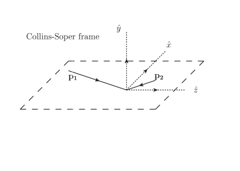
It is common to study the decaying lepton angular distribution in the Collins-Soper (CS) frame PhysRevD.16.2219 . The Collins-Soper frame, as shown in Fig.1, is a Z boson rest frame, with the z-axis lying in a way bisects the opening angle between the beam and negative target momenta directions. In this frame, momenta of the two incoming partons become:
| (5) | |||||
where the and dependences have been factorized out. Determined by these two momenta, the z-axis of this frame treats the in- and out-partons equally and is invariant under the longitudinal boost. This feature makes it suitable for the study of effects at finite . To avoid possible dilutions by the initial states swapped processes, we performed a rotation of around the x-axis for events with Aad:2016izn ; Khachatryan:2015paa . This rotation makes all angular coefficients distribute symmetric in .
In experiment, only the two decaying lepton pair are measurable, giving a set of visible variables , where the latter two denote polar and azimuthal angles of the charged lepton in the CS frame. We parametrize the Lorentz invariant phase space in a way such that the invisible part can be integrated over:
| (6) | |||||
| (8) | |||||
Then we factorize the decay angular distribution in terms of nine harmonic polynomials and eight angular coefficients Aad:2016izn ; Khachatryan:2015paa :
where the polar and azimuthal angles are measured in the CS frame. Coefficients are parity-odd and do not contribute at tree level and are found to be very small for a Z boson production Aad:2016izn ; Khachatryan:2015paa . Therefore in this analysis, we consider only .
3 Numerical results of angular coefficients in the Collins-Soper frame
As we are not directly searching for a resonance, the is expected to give no sensitivity and a narrow width approximation (NWA) is applied for convenience. Apart from that, we have four observables from the Z boson decay: . To study the features of this four-dimensional data, we calculate angular coefficients in the plane for both the major background process production and different dark sector models. The angular coefficients can be extracted using the method of moments Beaujean:2015xea . In the experiment, it is more straightforward to extract from a likelihood fit Aad:2016izn ; Khachatryan:2015paa .
Applying NWA for the Z boson, the cross section can be calculated through spin density matrices of the Z boson production () and decay ():
The Z boson production density matrix is defined in a specific range () of as follows:
| (10) | |||||
where means sum over spins and colors of all external particles other than the Z boson and averaged for the initial state ones. The decay density matrix is obtained using the Z boson decay amplitudes and parametrized similar as in Ref.Dutta:2008bh . The production and decay density matrices are both normalized such that the trace is one.
To obtain the amplitudes, we start from the FeynRules models implimented by authors of Ref.Mattelaer:2015haa ; Backovic:2015soa ; Neubert:2015fka ; Das:2016pbk ; Kraml:2017atm and use ALOHA in the MadGraph framework to generate HELAS subroutines for the helicity amplitudes Alloul:2013bka ; deAquino:2011ub ; Alwall:2014hca ; HAGIWARA19861 ; DREINER20101 . In the CS frame, we choose the z-axis as spin quantization axis, hence a rotation is necessary to bring the helicity frame results to the CS frame ones. We choose the y-axis to be common for the two frames and find the opening angle between the two frames can be obtained through
| (11) |
where and . The density matrices are then rotated according to Wigner’s d-functions:
| (12) | |||||
where we have used the following notations:
| (13) | |||||
| (17) |
The phase space is prepared analytically, and integration is performed using BASES Kawabata:1995th and GNU Scientific Library. We mapped the phase space variables to increase integration efficiencies. Specifically, for a massive propagator with mass m and width , the invariant mass is generated with
| (18) | |||||
| (19) | |||||
and is a uniformly generated random number.
The simulation considers , GeV, GeV and Patrignani:2016xqp . The W boson mass is obtained through , assuming parameter equals to one. The is chosen to be consistent with the one in the parton distribution functions (PDF). We use PDF set NNPDF23 Ball:2013hta with at leading order. The factorization scale is set to be equal to the Z boson transverse energy . Cross sections in this section consider the visible Z boson decays to electrons and muons with NWA and % Patrignani:2016xqp . The advantage of our program is that high statistical accuracy can be achieved through a direct integration. To validate our program, we checked our angular coefficients through toy measurements based on MadGraph5_aMC@NLO (MG5) generated events.
3.1 SM background
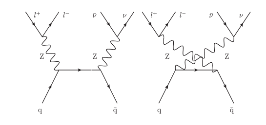
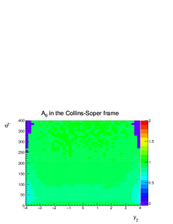
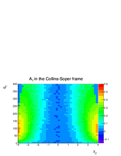
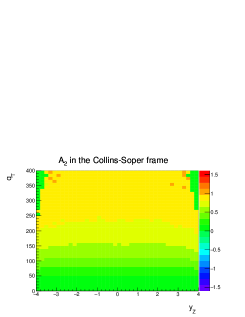
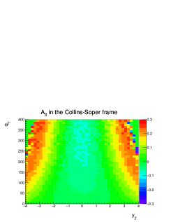
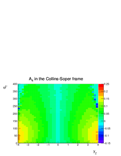
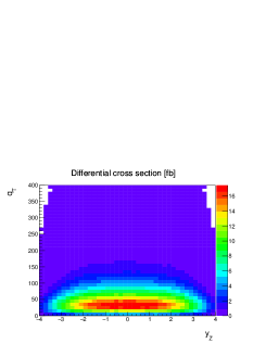
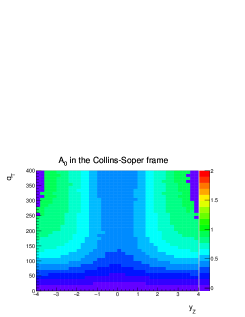
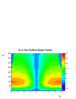
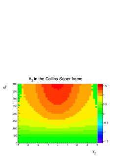
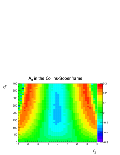
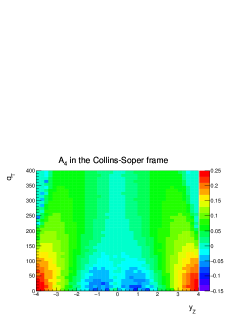
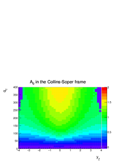
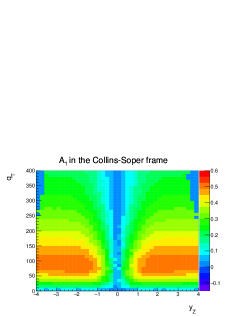
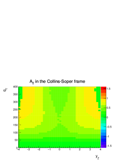
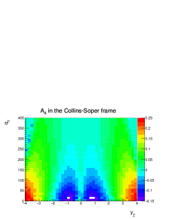
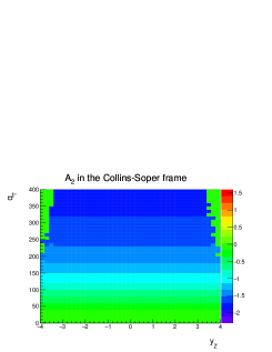
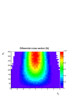
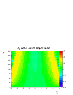
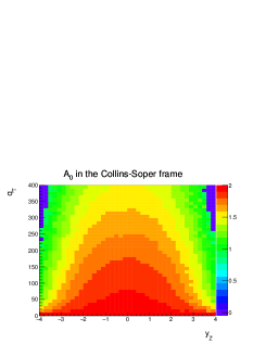
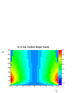
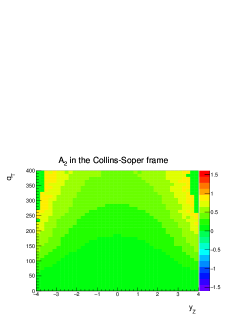
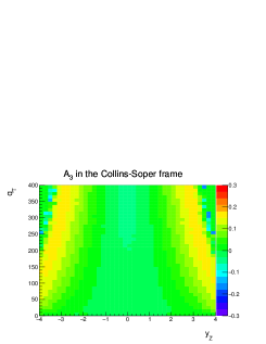
The SM production is the major background of our DM search. It has a similar final state signature as the signal process, as depicted in Fig. 2. Hence we first take a look at the Fig. 3 for the angular coefficients of this process. In general, the angular coefficient measures the difference between longitudinal and transverse polarizations, and it looks more longitudinal at high . The coefficient measures forward-backward asymmetry, the Z boson looks more like left-handed in the forward region. The measures the interference between the transverse amplitudes and the measures the interference between transverse and longitudinal.
3.2 Spin-0 mediator
We consider a simplified model with a scalar s-channel mediator as described in Ref. Neubert:2015fka . The dark sector model is constructed as follows:
| (21) | |||||
| (22) |
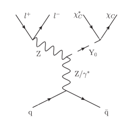
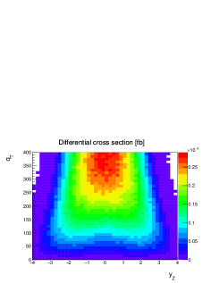
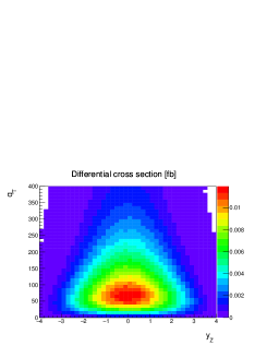
where is the dual field strength tensor of field, is a high energy scale. As discussed in Ref. Neubert:2015fka , this operator can be induced by a fermion loop graph with heavy fermion integrated out. Signature of this model is very different from the SM process, the dark mediator is emitted from the SM gauge bosons as depicted in Fig. 4. We consider three benchmark scenarios of the parameters labeled by S0a,b,c. As our angular distributions are more sensitive to changes in couplings, we fix the mass of dark matter GeV and the mass of the mediator GeV. The angular distributions won’t be changed drastically as long as is much smaller than . The parameter values and inclusive cross sections are listed in Table 1.
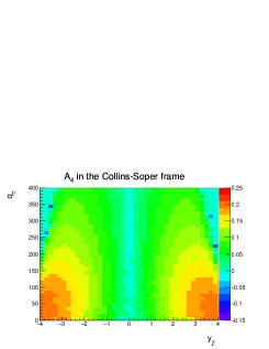
Angular coefficients of the benchmark scenatios S0a,b,c are shown in Fig. 5, Fig. 6 and Fig.7 respectively. Comparing to the SM , the dark matter signal is produced with much higher and have very different angular coefficients distributions, e.g., more transverse at low . The S0a and S0b can be distinguished from , where the dependences are very different. In the case of S0c, couples to weak bosons like a Higgs boson and cannot perturb the coupling structure with the Z boson production. Consequently, the , and in the CS frame are all zero hence are not shown in the figure.
| Benchmark | S0a | S0b | S0c |
|---|---|---|---|
| 1 | 0 | 0 | |
| 0 | 1 | 0 | |
| 0 | 0 | 1 | |
| 0.25 | 0 | 0 | |
| 0 | 0.25 | 0 | |
| 0 | 0 | 1 | |
| (GeV) | 3000 | 3000 | 3000 |
| Interaction | CP-even | CP-odd | CP-even |
| (GeV) | 10 | 10 | 10 |
| (GeV) | 1000 | 1000 | 1000 |
| (GeV) | 41.4 | 41.4 | 1.05 |
| Cross section (fb) | 0.0103 | 0.00977 | 2.98e-08 |


3.3 Spin-1 mediator
We consider the same dark sector with a spin-1 mediator as in the LHC experiment Abercrombie:2015wmb with the following interactions of the dark sector:
| (23) | |||||
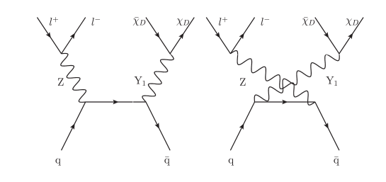
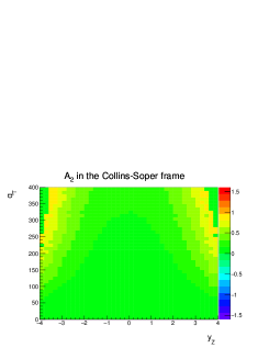
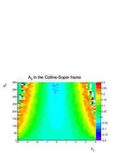
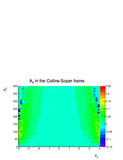
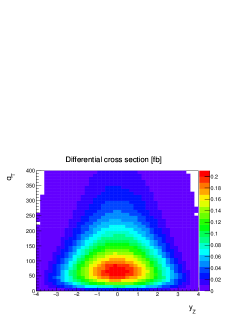
The masses of the dark matter and the mediator are chosen to be the same as in the spin-0 model. A sound discussion of the impact of the choice of masses is available in the Ref. Abercrombie:2015wmb . Since our analysis is more suitable for testing couplings, we consider benchmark scenarios as listed in Table 2. The signal signature is close to the SM process, as shown in Fig. 8, and we include here the SM as a special case with zero coupling for comparison. The S1b and S1c project out the right- and left-handed part the Z-q- couplings. Since the magnitude of the left-handed couplings are larger than the one of the right-handed, cross section of the S1c scenario is found to be much larger than the S1b scenario.
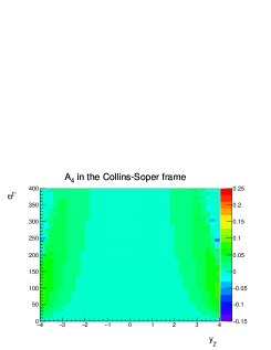
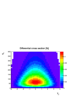
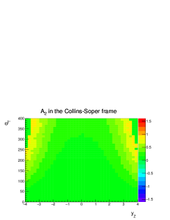
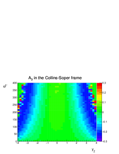
Angular coefficients of the benchmark scenarios S1a,b,c are shown in Fig. 9, Fig. 10 and Fig. 11 respectively. Comparing with the SM and spin-0 dark sector models, of the spin-1 models are found to be very significant. Among the three scenarios, most signatures look similar, but and take different signs between the S1b and S1c. Hence the and can be used to quantify the parity violation of the dark sector.
| Benchmark | S1a | S1b | S1c | S10 |
| Spin independent | Right handed | Left handed | SM () | |
| 1 | - | |||
| 0 | - | - | ||
| 0 | 0 | 0 | - | |
| 0.25 | - | |||
| 0 | - | - | ||
| 0.25 | - | |||
| 0 | - | - | ||
| (GeV) | 10 | 10 | 10 | - |
| (GeV) | 1000 | 1000 | 1000 | - |
| (GeV) | 56.3 | 55.9 | 55.9 | - |
| Cross section (fb) | 2.50 | 0.533 | 4.50 | 239 |




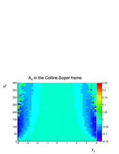
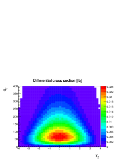
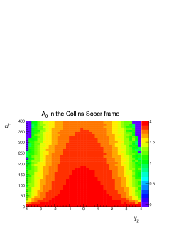
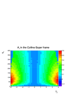
3.4 Spin-2 mediator
The dark sector with a spin-2 mediator is also tested. We consider a model as described in the Ref.Kraml:2017atm , with benchmark scenarios listed in Table 3. The masses of the dark matter and the mediator are also chosen to be the same as in the spin-0 model. Despite an increase of complexity in the computation, we found the angular coefficients look similar to the benchmark scenario S1a. We show only the angular coefficients of the benchmark scenario S2a in Fig. 12. Some visible differences from the S1a can be observed from the and distributions. Since we do not measure the DM, the angular coefficients of S2b,c are found to be very close to the ones of S2a.
| Benchmark | S2a | S2b | S2c |
|---|---|---|---|
| 1 | 0 | 0 | |
| 0 | 1 | 0 | |
| 0 | 0 | 1 | |
| 1 | 1 | 1 | |
| (GeV) | 10 | 10 | 10 |
| (GeV) | 1000 | 1000 | 1000 |
| 3000 | 3000 | 3000 | |
| (GeV) | 95.3 | 93.7 | 97.7 |
| Cross section (fb) | 2.73 | 0.0462 | 0.578 |

4 Setting limits on the coupling strength parameters of dark sector models
In Section 3, we have shown that angular coefficients of the benchmark dark sector models can have distinct signatures from the SM background process in the plane. In this section, we take advantage of these signatures and set limit on the coupling strength parameter of each dark sector model, based on observables . The invisible part was integrated out to construct pdfs, as described in Section 2.
4.1 Statistical method
With the pdfs of the signal and background processes obtained through MEM, one can construct an unbinned likelihood function over N events in the data sample Barlow:1990vc :
| (24) | |||||
| (25) |
where and represent pdfs of the signal and background, and corresponding to the expected signal and background yields. The represents the full set of nuisance parameters with pdf , which are designed to incorporate systematic uncertainties.
To set limits on the parameters , we compare the compatibility of the data with the fixed and floated hypotheses and construct a test statistic based on the profile likelihood ratio:
| (26) |
According to the Wilk’s theorem, this test statistic satisfies the distribution of the same degrees of freedom as in the large sample limit wilks1938 . One can, therefore, set limits on the through a parameter space scan and cut on the values.
Neglecting pdf of the nuisance parameters, it follows that
| (27) |
For setting limits on , we assume that there is a single dataset in agreement with . In the large sample limit, we have:
where the first term is a test statistic for simple counting experiment and the second term is proportional to and a KL-divergence kullback1951 . As the KL-divergence measures the difference of the pdfs and , it quantifies the powerfulness of the MEM. For simplicity, we will call the first term as normalization term and the second one as KL-divergence term.
In our study, the likelihood function is prepared by BASES numerical integration with HELAS subroutines for the helicity amplitudes. The evaluation of the KL-divergence term is performed using a plain integration provided by the GNU Scientific Library. We validate our program by checking the normalizations of all the constructed pdfs and by comparing the angular coefficients and cross sections of all involved processes with the MG5. See more information in Appendix A.
4.2 Background modeling and event selections
To make our limits more realistic, we consider a few selections – marked as BL selections – as listed in Table 4 to capture major detector acceptance effects for the processes involved. The values of these selections are set refering to recent 13 TeV LHC measurements Sirunyan:2017onm ; Aaboud:2017bja . There are several additional selections considered in experiments to improve the signal feasibility, e.g., jet counting, -lepton veto, top quark veto, and , for momentum balance Sirunyan:2017onm . These selections reject most background from misidentification but lead to different acceptance efficiencies for different processes. Without detector simulation, we determine the event rate according to the CMS results (Table 3 of Ref. Sirunyan:2017onm ), with an ancillary incorporating the additional selections in the experiment and a scale factor normalizing to 150 data. The signal dark matter processes are assumed to have the same ancillary as the SM ZZ process.
| Variable | Requirements |
|---|---|
| GeV | |
| NWA | |
| GeV | |
Our background pdf is constructed based on components summarized in Table 5. Apart from the non-resonant- background, which is constructed using only the phase space, other components are built using matrix elements. The WZ matrix element assumes W, where the electron is not identified by a detector. The Z/ is estimated with matrix element of the Z plus one jet production, phase space of this process reduces to three final state particles.
| Process | Cross section with BL-selections (fb) | Ancillary | Events |
|---|---|---|---|
| ZZ | 27.7 | 0.488 | 2028 |
| Non-resonant- | 1.57 | 5.80 | 1370 |
| WZ() | 17.05 | 0.296 | 757 |
| Z/ | 3.61 | 1.23 | 665 |
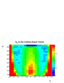
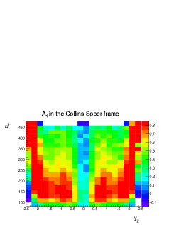
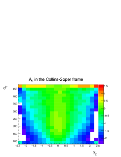
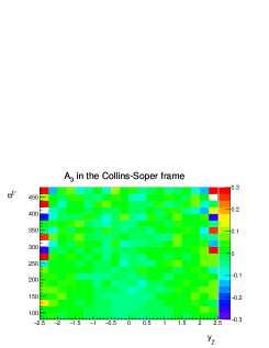
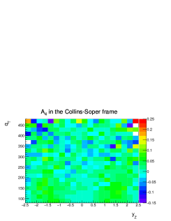
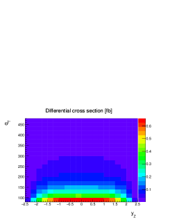
In the presence of selections, angular coefficients can be distorted. Fig. 13 shows the angular coefficients for the background only hypothesis. Irregular distributions on the boundaries are mainly caused by the selections on and . With the coupling strength at our expected limit, the presence of signal can only perturb the shapes of the background only ones.
4.3 Limits on the coupling strength parameters of the dark sector models
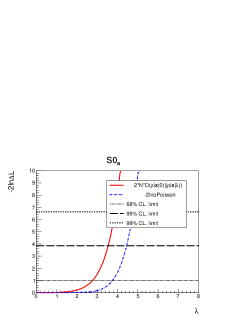
In our dark sector models, it is necessary to have two couplings: one for the interaction with SM particles, one for the DM decay. For conciseness, we assume that both couplings in the benchmark model are scaled by a strength parameter . This assumption makes the cross sections change with two orders severer in couplings than ones for limits of a single coupling. We compare the upper limits set from the normalization term and from the KL-divergence term in Fig. 14 for the S0 benchmark scenarios and in Fig. 15 for the S1 benchmark scenarios. The shapes provide significant improvements in all cases. The KL-divergence terms drive the final limits for the S0 benchmark scenarios and are close to the normalization terms in the S1 benchmark scenarios.
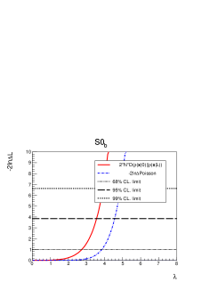
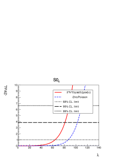

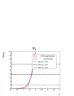
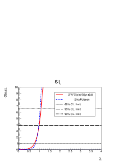
We provide in Table 6 95% CL upper limits of the strength parameters. In our evaluation, the numerical uncertainty of the normalization terms can be easily made negligible. However, the evaluation of the KL-divergence terms can be computationally expensive. It takes us roughly CPU hours, functioning at about 2.4 GHz, for us to obtain 30%-50% uncertainties on the KL-divergence terms around the limit values. The signal cross sections at the limit values are also reported. Since a counting experiment calculate limits based on signal background yields, the results from the normalization term are almost the same. The ones from the KL-divergence terms, however, depend on the shape difference between the signal and background. As the KL-divergence is a measure the shape difference, a lower cross section means a larger the difference in shape. These quantitative results are in agreement with qualitative features of the angular coefficients among models provided in Section 3.
| Benchmark | S0a | S0b | S0c | S1a | S1b | S1c |
| Limit from the normalization term () | 4.4 | 4.6 | 103 | 1.1 | 1.7 | 0.97 |
| Signal cross section at (fb) | 1.86 | 1.87 | 1.86 | 1.87 | 1.87 | 1.87 |
| Limit from the KL-divergence term () | 3.5 | 3.6 | 81 | 1.1 | 1.7 | 0.99 |
| Signal cross section at (fb) | 0.75 | 0.70 | 0.72 | 1.9 | 2.0 | 2.0 |
| Combined limit () | 3.5 | 3.5 | 79 | 1.0 | 1.5 | 0.89 |
4.4 Example application of MEKD
Our computation considered only parton level matrix element at leading order (LO). We comment that there are already efforts to extend the MEM to Next-to-Leading Order (NLO) Campbell:2012cz and incorporates parton shower effects Soper:2011cr . There is an easier approach to exploit the LO matrix elements, called the matrix element kinematic discriminator (MEKD) Avery:2012um ; Chatrchyan:2012sn ; Chatrchyan:2012jja . This method construct a variable named MEKD that can be calculated for events with required observables. By construction, it utilizes the matrix element and can be used to distinguish the signal and background. The advantage of this method is that detector effects and theoretical uncertainties in the construction of likelihood function is independent of the application.
Based on the pdfs defined as in Eq. 1 of the signal and combined background, we define the MEKD as:
| (29) |
where and the invisible part has been integrated out. Then we use the MG5 program to generate events for the applications. For the LO simulations, we consider the same setup as has been used in our program. For the NLO simulations, we consider NNPDF23_nlo with default renormalization and factorization scales, defined as the sum of the transverse masses divided by two of all final state particles and partons. Negatively weighted events in the NLO simulations have been incorporated consistently.
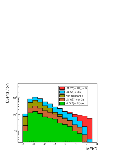
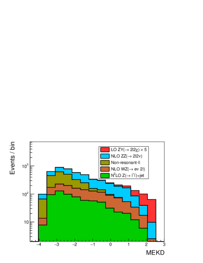
The Fig. 16 stacks MEKD distributions of both signal and backgrounds. On the left plot, all of the processes are generated with LO accuracy (NLO in QCD for Z()+jet). The signal considers S0a benchmark model with . We multiplied the signal yield by a factor of five for a better demonstration. The Non-resonant- process is expected to be obtained from data-driven in the experiment. We mimic its contribution by using a sample. The right plot replaces the SM ZZ, WZ() and Z()+jet with simulated events at NLO accuracy. In both cases, the MEKD shows very nice discrimination power on the signal and background. It is made clear that NLO simulated events are applicable, with a reasonable loss of sensitivity.
5 Summary
In this paper, we have exploited the Z boson leptonic decay information to probe the dark sector with a scalar, vector, and tensor mediators. We obtained angular coefficients of the SM background and benchmark scenarios of the dark sector models in the plane. Our results show that the angular coefficients behave very differently between the SM process and the dark sector signal processes. The angular coefficients among dark sector models of spin-0 and spin-1 mediators are also found to be different from scenario to scenario. Specifically, the angular coefficients have sensitivities on the parity violation of the spin-1 model and the CP-violation of the spin-0 model. The angular coefficients in the spin-2 model are found to be similar to the spin-independent scenario of the spin-1 model but still have minor differences.
To quantify the shape information that can be used for the search of dark sectors, we consider unbinned fits to the four-dimensional distributions based on dynamically constructed matrix element likelihood functions and set 95% CL upper limits on the coupling strength parameters of the spin-0 and spin-1 benchmark scenarios. To be realistic, we emulate the acceptance and efficiency effects referring to the 13 TeV LHC measurement Sirunyan:2017onm ; Aaboud:2017bja . To make our framework concise, we obtained all the results using asymptotic approximation without event generation.
Our evaluated KL-divergence term quantifies the shape effect in each case. The obtained results demonstrate significant improvements in the limits, especially on the S0 benchmark models. For easier usage of experimental data, we provide an example application of MEKD with simulated events. We show that our MEKD constructed with LO matrix elements are applicable for NLO events and preserves good discrimination power on the signal and background. We expect this kind of MEKDs to be useful for exploiting the lepton angular distributions in experimental analyses.
Acknowledgments
This work would not be possible without what D. Yang have learned from Kaoru Hagiwara (KEK) back in PITT PACC (U.S.) and Xinjiang Univ. (China). We have benefited from useful discussions with many people, to name a few, Kaoru Hagiwara, Tao Han, Junmo Chen, Xing Wang (PITT), Kai Ma (SUT) and Yandong Liu, Jing Li (PKU). D. Yang would also like to thank the PITT particle physics group and the Xinjiang Univ. theoretical physics group for warm hospitality during the stay. We are also grateful to Junichi Kanzaki (KEK), Yajuan Zheng (NTU) for useful advises in using BASES. This work is supported in part by the National Natural Science Foundation of China, under Grants No. 11475190 and No. 1157500, and by a short-term internship program from the graduate school of Peking University.
Appendix A Cross checks with the MG5 program
To make the MG5 results comparable, we implemented similar setups as described in the paper. These include coupling constants, the choice of PDF set, renormalization and factorization scales, Breit-Wigner cutoff, and BL selections as described in Table 4 of the paper. The Table 7 compares our results with the MG5 ones with one on-shell Z boson in the final states. For all the cases, the differences lie within statistical uncertainty. The Table 8 compares our results with the MG5 with the Z boson leptonicalled decayed. Our program considered all the BL-selections with NWA, while the MG5 ones replace the NWA with . This replacement leads to slightly smaller MG5 cross sections comparing to ours, but in general, the differences are not large. Normalizations of the signal and all of the background pdfs are also checked to be consistent with one.
| Process/Benchmark | Cross section | Cross section | Relative | Relative |
| (fb) | from MG5 (fb) | Difference (%) | Statistical uncertainty (%) | |
| S0a | 0.1535 | 0.1536 | 0.052 | 0.34 |
| S0b | 0.1452 | 0.1454 | 0.14 | 0.29 |
| S0c | 4.436 | 4.459 | 0.52 | 0.14 |
| S1a | 37.16 | 37.21 | 0.14 | 0.23 |
| S1b | 7.931 | 7.943 | 0.15 | 0.24 |
| S1c | 66.94 | 67.01 | 0.11 | 0.25 |
| Z()Z | 3561 | 3564 | 0.081 | 0.16 |
| W()Z | 2547 | 2556 | 0.39 | 0.26 |
| Z+jet | 1.189 | 1.192 | 0.23 | 0.23 |
| Process/Benchmark | Cross section | Cross section | Relative | Relative |
| (fb) | from MG5 (fb) | Difference (%) | Statistical uncertainty (%) | |
| S0a | 4.748 | 4.688 | 1.3 | 0.31 |
| S0b | 4.333 | 4.382 | 1.1 | 0.33 |
| S0c | 1.667 | 1.649 | 1.1 | 0.27 |
| S1a | 1.149 | 1.034 | 11 | 0.23 |
| S1b | 0.2431 | 0.2186 | 11 | 0.27 |
| S1c | 2.070 | 1.861 | 11 | 0.23 |
| ZZ | 27.71 | 26.50 | 4.6 | 0.13 |
| WZ() | 17.05 | 18.39 | 7.3 | 0.26 |
| Z()+jet | 36125 | 34440 | 4.9 | 0.30 |
References
- (1) Particle Data Group collaboration, C. Patrignani et al., Review of Particle Physics, Chin. Phys. C40 (2016) 100001.
- (2) Planck collaboration, P. A. R. Ade et al., Planck 2015 results. XIII. Cosmological parameters, Astron. Astrophys. 594 (2016) A13, [1502.01589].
- (3) B. W. Lee and S. Weinberg, Cosmological lower bound on heavy-neutrino masses, Phys. Rev. Lett. 39 (Jul, 1977) 165–168.
- (4) M. Beltran, D. Hooper, E. W. Kolb, Z. A. C. Krusberg and T. M. P. Tait, Maverick dark matter at colliders, JHEP 09 (2010) 037, [1002.4137].
- (5) ATLAS collaboration, M. Aaboud et al., Measurement of detector-corrected observables sensitive to the anomalous production of events with jets and large missing transverse momentum in collisions at TeV using the ATLAS detector, 1707.03263.
- (6) CMS collaboration, A. M. Sirunyan et al., Search for dark matter produced with an energetic jet or a hadronically decaying W or Z boson at TeV, JHEP 07 (2017) 014, [1703.01651].
- (7) ATLAS collaboration, M. Aaboud et al., Search for dark matter produced in association with bottom or top quarks in = 13 TeV pp collisions with the ATLAS detector, 1710.11412.
- (8) CMS collaboration, A. M. Sirunyan et al., Search for dark matter produced in association with heavy-flavor quarks in proton-proton collisions at sqrt(s)=13 TeV, 1706.02581.
- (9) CMS collaboration, A. M. Sirunyan et al., Search for new physics in the monophoton final state in proton-proton collisions at TeV, JHEP 10 (2017) 073, [1706.03794].
- (10) L. M. Carpenter, A. Nelson, C. Shimmin, T. M. P. Tait and D. Whiteson, Collider searches for dark matter in events with a Z boson and missing energy, Phys. Rev. D87 (2013) 074005, [1212.3352].
- (11) CMS collaboration, A. M. Sirunyan et al., Search for dark matter and unparticles in events with a Z boson and missing transverse momentum in proton-proton collisions at TeV, JHEP 03 (2017) 061, [1701.02042].
- (12) ATLAS collaboration, M. Aaboud et al., Search for an invisibly decaying Higgs boson or dark matter candidates produced in association with a boson in collisions at 13 TeV with the ATLAS detector, 1708.09624.
- (13) Y. Bai and T. M. P. Tait, Searches with Mono-Leptons, Phys. Lett. B723 (2013) 384–387, [1208.4361].
- (14) ATLAS collaboration, M. Aaboud et al., Search for a new heavy gauge boson resonance decaying into a lepton and missing transverse momentum in 36 fb-1 of collisions at 13 TeV with the ATLAS experiment, 1706.04786.
- (15) ATLAS collaboration, M. Aaboud et al., Search for Dark Matter Produced in Association with a Higgs Boson Decaying to using 36 fb-1 of collisions at TeV with the ATLAS Detector, Phys. Rev. Lett. 119 (2017) 181804, [1707.01302].
- (16) CMS collaboration, A. M. Sirunyan et al., Search for associated production of dark matter with a Higgs boson decaying to or at = 13 TeV, 1703.05236.
- (17) CMS collaboration, A. M. Sirunyan et al., Search for dijet resonances in proton¿proton collisions at = 13 TeV and constraints on dark matter and other models, Phys. Lett. B769 (2017) 520–542, [1611.03568].
- (18) CMS collaboration, V. Khachatryan et al., Search for heavy gauge W’ boson in events with an energetic lepton and large missing transverse momentum at 13 TeV, Phys. Lett. B770 (2017) 278–301, [1612.09274].
- (19) CMS collaboration, A. M. Sirunyan et al., Search for low mass vector resonances decaying into quark-antiquark pairs in proton-proton collisions at 13 TeV, 1710.00159.
- (20) ATLAS collaboration, M. Aaboud et al., Search for new high-mass phenomena in the dilepton final state using 36.1 fb-1 of proton-proton collision data at = 13 TeV with the ATLAS detector, 1707.02424.
- (21) D. Abercrombie et al., Dark Matter Benchmark Models for Early LHC Run-2 Searches: Report of the ATLAS/CMS Dark Matter Forum, 1507.00966.
- (22) M. Neubert, J. Wang and C. Zhang, Higher-Order QCD Predictions for Dark Matter Production in Mono- Searches at the LHC, JHEP 02 (2016) 082, [1509.05785].
- (23) F. J. Petriello, S. Quackenbush and K. M. Zurek, The Invisible at the CERN LHC, Phys. Rev. D77 (2008) 115020, [0803.4005].
- (24) A. Alves and K. Sinha, Searches for Dark Matter at the LHC: A Multivariate Analysis in the Mono- Channel, Phys. Rev. D92 (2015) 115013, [1507.08294].
- (25) T. Han, D. L. Rainwater and D. Zeppenfeld, Drell-Yan plus missing energy as a signal for extra dimensions, Phys. Lett. B463 (1999) 93–98, [hep-ph/9905423].
- (26) Z.-H. Yu, X.-J. Bi, Q.-S. Yan and P.-F. Yin, Dark matter searches in the mono- channel at high energy colliders, Phys. Rev. D90 (2014) 055010, [1404.6990].
- (27) ATLAS collaboration, G. Aad et al., Search for contact interactions and large extra dimensions in the dilepton channel using proton-proton collisions at = 8 TeV with the ATLAS detector, Eur. Phys. J. C74 (2014) 3134, [1407.2410].
- (28) J. Goodman, M. Ibe, A. Rajaraman, W. Shepherd, T. M. P. Tait and H.-B. Yu, Constraints on Dark Matter from Colliders, Phys. Rev. D82 (2010) 116010, [1008.1783].
- (29) J. Goodman, M. Ibe, A. Rajaraman, W. Shepherd, T. M. P. Tait and H.-B. Yu, Constraints on Light Majorana dark Matter from Colliders, Phys. Lett. B695 (2011) 185–188, [1005.1286].
- (30) Q.-H. Cao, C.-R. Chen, C. S. Li and H. Zhang, Effective Dark Matter Model: Relic density, CDMS II, Fermi LAT and LHC, JHEP 08 (2011) 018, [0912.4511].
- (31) R. C. Cotta, J. L. Hewett, M. P. Le and T. G. Rizzo, Bounds on Dark Matter Interactions with Electroweak Gauge Bosons, Phys. Rev. D88 (2013) 116009, [1210.0525].
- (32) O. Mattelaer and E. Vryonidou, Dark matter production through loop-induced processes at the LHC: the s-channel mediator case, Eur. Phys. J. C75 (2015) 436, [1508.00564].
- (33) M. Backovic, M. Krämer, F. Maltoni, A. Martini, K. Mawatari and M. Pellen, Higher-order QCD predictions for dark matter production at the LHC in simplified models with s-channel mediators, Eur. Phys. J. C75 (2015) 482, [1508.05327].
- (34) G. Das, C. Degrande, V. Hirschi, F. Maltoni and H.-S. Shao, NLO predictions for the production of a spin-two particle at the LHC, Phys. Lett. B770 (2017) 507–513, [1605.09359].
- (35) S. Kraml, U. Laa, K. Mawatari and K. Yamashita, Simplified dark matter models with a spin-2 mediator at the LHC, Eur. Phys. J. C77 (2017) 326, [1701.07008].
- (36) K. Cheung, K. Mawatari, E. Senaha, P.-Y. Tseng and T.-C. Yuan, The Top Window for dark matter, JHEP 10 (2010) 081, [1009.0618].
- (37) T. Lin, E. W. Kolb and L.-T. Wang, Probing dark matter couplings to top and bottom quarks at the LHC, Phys. Rev. D88 (2013) 063510, [1303.6638].
- (38) K. Kondo, Dynamical likelihood method for reconstruction of events with missing momentum. i. method and toy models, Journal of the Physical Society of Japan 57 (1988) 4126–4140, [http://dx.doi.org/10.1143/JPSJ.57.4126].
- (39) K. Kondo, Dynamical likelihood method for reconstruction of events with missing momentum. ii. mass spectra for 22 processes, Journal of the Physical Society of Japan 60 (1991) 836–844, [http://dx.doi.org/10.1143/JPSJ.60.836].
- (40) Y. Gao, A. V. Gritsan, Z. Guo, K. Melnikov, M. Schulze and N. V. Tran, Spin determination of single-produced resonances at hadron colliders, Phys. Rev. D81 (2010) 075022, [1001.3396].
- (41) CMS collaboration, S. Chatrchyan et al., Search for a Higgs boson in the decay channel to ZZ(*) to qbar l+ in collisions at TeV, JHEP 04 (2012) 036, [1202.1416].
- (42) A. De Rujula, J. Lykken, M. Pierini, C. Rogan and M. Spiropulu, Higgs look-alikes at the LHC, Phys. Rev. D82 (2010) 013003, [1001.5300].
- (43) S. Kullback and R. A. Leibler, On information and sufficiency, Ann. Math. Statist. 22 (03, 1951) 79–86.
- (44) J. Alwall, A. Freitas and O. Mattelaer, The Matrix Element Method and QCD Radiation, Phys. Rev. D83 (2011) 074010, [1010.2263].
- (45) J. C. Collins and D. E. Soper, Angular distribution of dileptons in high-energy hadron collisions, Phys. Rev. D 16 (Oct, 1977) 2219–2225.
- (46) ATLAS collaboration, G. Aad et al., Measurement of the angular coefficients in -boson events using electron and muon pairs from data taken at TeV with the ATLAS detector, JHEP 08 (2016) 159, [1606.00689].
- (47) CMS collaboration, V. Khachatryan et al., Angular coefficients of Z bosons produced in pp collisions at = 8 TeV and decaying to as a function of transverse momentum and rapidity, Phys. Lett. B750 (2015) 154–175, [1504.03512].
- (48) F. Beaujean, M. Chrzaszcz, N. Serra and D. van Dyk, Extracting Angular Observables without a Likelihood and Applications to Rare Decays, Phys. Rev. D91 (2015) 114012, [1503.04100].
- (49) S. Dutta, K. Hagiwara and Y. Matsumoto, Measuring the Higgs-Vector boson Couplings at Linear Collider, Phys. Rev. D78 (2008) 115016, [0808.0477].
- (50) A. Alloul, N. D. Christensen, C. Degrande, C. Duhr and B. Fuks, FeynRules 2.0 - A complete toolbox for tree-level phenomenology, Comput. Phys. Commun. 185 (2014) 2250–2300, [1310.1921].
- (51) P. de Aquino, W. Link, F. Maltoni, O. Mattelaer and T. Stelzer, ALOHA: Automatic Libraries Of Helicity Amplitudes for Feynman Diagram Computations, Comput. Phys. Commun. 183 (2012) 2254–2263, [1108.2041].
- (52) J. Alwall, R. Frederix, S. Frixione, V. Hirschi, F. Maltoni, O. Mattelaer et al., The automated computation of tree-level and next-to-leading order differential cross sections, and their matching to parton shower simulations, JHEP 07 (2014) 079, [1405.0301].
- (53) K. Hagiwara and D. Zeppenfeld, Helicity amplitudes for heavy lepton production in e+e annihilation, Nuclear Physics B 274 (1986) 1 – 32.
- (54) H. K. Dreiner, H. E. Haber and S. P. Martin, Two-component spinor techniques and feynman rules for quantum field theory and supersymmetry, Physics Reports 494 (2010) 1 – 196.
- (55) S. Kawabata, A New version of the multidimensional integration and event generation package BASES/SPRING, Comput. Phys. Commun. 88 (1995) 309–326.
- (56) NNPDF collaboration, R. D. Ball, V. Bertone, S. Carrazza, L. Del Debbio, S. Forte, A. Guffanti et al., Parton distributions with QED corrections, Nucl. Phys. B877 (2013) 290–320, [1308.0598].
- (57) R. J. Barlow, Extended maximum likelihood, Nucl. Instrum. Meth. A297 (1990) 496–506.
- (58) S. S. Wilks, The large-sample distribution of the likelihood ratio for testing composite hypotheses, Ann. Math. Statist. 9 (03, 1938) 60–62.
- (59) J. M. Campbell, W. T. Giele and C. Williams, The Matrix Element Method at Next-to-Leading Order, JHEP 11 (2012) 043, [1204.4424].
- (60) D. E. Soper and M. Spannowsky, Finding physics signals with shower deconstruction, Phys. Rev. D84 (2011) 074002, [1102.3480].
- (61) P. Avery et al., Precision studies of the Higgs boson decay channel HZZ4 with MEKD, Phys. Rev. D87 (2013) 055006, [1210.0896].
- (62) CMS collaboration, S. Chatrchyan et al., Study of the Mass and Spin-Parity of the Higgs Boson Candidate Via Its Decays to Z Boson Pairs, Phys. Rev. Lett. 110 (2013) 081803, [1212.6639].