On the Spectral Resolution of Products
of Laplacian Eigenfunctions

Stefan Steinerberger Department of Mathematics, Yale University, New Haven, CT 06511, USA stefan.steinerberger@yale.edu
Abstract.

We study products of eigenfunctions of the Laplacian Δϕλ=λϕλΔsubscriptitalic-ϕ𝜆𝜆subscriptitalic-ϕ𝜆-\Delta\phi_{\lambda}=\lambda\phi_{\lambda} on compact manifolds. If ϕμ,ϕλsubscriptitalic-ϕ𝜇subscriptitalic-ϕ𝜆\phi_{\mu},\phi_{\lambda} are two eigenfunctions and μλ𝜇𝜆\mu\leq\lambda, then one would perhaps expect their product ϕμϕλsubscriptitalic-ϕ𝜇subscriptitalic-ϕ𝜆\phi_{\mu}\phi_{\lambda} to be mostly a linear combination of eigenfunctions with eigenvalue close to λ𝜆\lambda. This can faily quite dramatically: on 𝕋2superscript𝕋2\mathbb{T}^{2}, we see that

2sin(nx)sin((n+1)x)=cos(x)cos((2n+1)x)2𝑛𝑥𝑛1𝑥𝑥2𝑛1𝑥2\sin{(nx)}\sin{((n+1)x)}=\cos{(x)}-\cos{((2n+1)x)}

has half of its L2limit-fromsuperscript𝐿2L^{2}-mass at eigenvalue 1. Conversely, the product

sin(nx)sin(my)lives at eigenvaluemax{m2,n2}m2+n22max{m2,n2}𝑛𝑥𝑚𝑦lives at eigenvaluesuperscript𝑚2superscript𝑛2superscript𝑚2superscript𝑛22superscript𝑚2superscript𝑛2\sin{(nx)}\sin{(my)}\qquad\mbox{lives at eigenvalue}\quad\max{\left\{m^{2},n^{2}\right\}}\leq m^{2}+n^{2}\leq 2\max{\left\{m^{2},n^{2}\right\}}

and the heuristic is valid. We show that the main reason is that in the first example ’the waves point in the same direction’: if the heuristic fails and multiplication carries L2limit-fromsuperscript𝐿2L^{2}-mass to lower frequencies, then ϕμsubscriptitalic-ϕ𝜇\phi_{\mu} and ϕλsubscriptitalic-ϕ𝜆\phi_{\lambda} are strongly correlated at scale λ1/2similar-toabsentsuperscript𝜆12\sim\lambda^{-1/2} (the shorter wavelength)

Mp(t,x,y)(ϕλ(y)ϕλ(x))(ϕμ(y)ϕμ(x))𝑑yLx2ϕμϕλL2,greater-than-or-equivalent-tosubscriptnormsubscript𝑀𝑝𝑡𝑥𝑦subscriptitalic-ϕ𝜆𝑦subscriptitalic-ϕ𝜆𝑥subscriptitalic-ϕ𝜇𝑦subscriptitalic-ϕ𝜇𝑥differential-d𝑦subscriptsuperscript𝐿2𝑥subscriptnormsubscriptitalic-ϕ𝜇subscriptitalic-ϕ𝜆superscript𝐿2\left\|\int_{M}{p(t,x,y)(\phi_{\lambda}(y)-\phi_{\lambda}(x))(\phi_{\mu}(y)-\phi_{\mu}(x))dy}\right\|_{L^{2}_{x}}\gtrsim\|\phi_{\mu}\phi_{\lambda}\|_{L^{2}},

where p(t,x,y)𝑝𝑡𝑥𝑦p(t,x,y) is the classical heat kernel and tλ1similar-to𝑡superscript𝜆1t\sim\lambda^{-1}. This turns out to be a fairly fundamental principle and is even valid for the Hadamard product of eigenvectors of a Graph Laplacian.

Key words and phrases:
Laplacian eigenfunctions, triple product, local correlation, quantum chaos.
2010 Mathematics Subject Classification:
35B05, 35J05 (primary) and 81Q50 (secondary)

1. Introduction and main results

1.1. Introduction.

We start by considering Laplacian eigenfunctions Δϕλ=λϕλΔsubscriptitalic-ϕ𝜆𝜆subscriptitalic-ϕ𝜆-\Delta\phi_{\lambda}=\lambda\phi_{\lambda} on smooth, compact Riemannian manifolds with or without boundary (and Dirichlet or Neumann conditions in the case of a boundary). Ultimately, the results are so general that they will easily transfer to the case of finite graphs equipped with a Graph Laplacian. We consider a basic question.

Question. What is the behavior of the spectral resolution of the product ϕμϕλsubscriptitalic-ϕ𝜇subscriptitalic-ϕ𝜆\phi_{\mu}\phi_{\lambda}?

Except for the special case where additional structure is present (see for example Sarnak [26], Bernstein & Reznikoff [3] and Krötz & Stanton [19]), there seem to be very few results in the literature. Already the L2limit-fromsuperscript𝐿2L^{2}-size of the product is a highly nontrivial quantity: a seminal result due to Burq-Gérard-Tzetkov [6] establishes

ϕμϕλL2min(λ,μ)ϕλL2ϕμL2less-than-or-similar-tosubscriptnormsubscriptitalic-ϕ𝜇subscriptitalic-ϕ𝜆superscript𝐿2𝜆𝜇subscriptnormsubscriptitalic-ϕ𝜆superscript𝐿2subscriptnormsubscriptitalic-ϕ𝜇superscript𝐿2\|\phi_{\mu}\phi_{\lambda}\|_{L^{2}}\lesssim\min(\sqrt{\lambda},\sqrt{\mu})\|\phi_{\lambda}\|_{L^{2}}\|\phi_{\mu}\|_{L^{2}}

on compact two-dimensional manifolds without boundary (the same authors extended the result to higher dimensions [7]). Similar results were established on two- and three-dimensional manifolds with boundary by Blair, Smith & Sogge [5]. The problem of obtaining more informative bounds on ϕμϕλ,ϕνsubscriptitalic-ϕ𝜇subscriptitalic-ϕ𝜆subscriptitalic-ϕ𝜈\left\langle\phi_{\mu}\phi_{\lambda},\phi_{\nu}\right\rangle is clearly fairly fundamental by itself but also occurs somewhat frequently in applications (see e.g. [17, 24, 25] for problems arising in dimensionality reduction of high-dimensional data or [22] for pattern matching of deformable shapes). The problem is trivial on the torus 𝕋dsuperscript𝕋𝑑\mathbb{T}^{d} but already on 𝕊2superscript𝕊2\mathbb{S}^{2} the arising integrals involve Clebsch-Gordon coefficients and are deeply connected to concepts in representation theory.

1.2. A Napkin Computation

This section contains a very heuristic derivation of how one would hope to describe the phenomenon. We shall assume that μλ𝜇𝜆\mu\leq\lambda throughout the paper and start with a basic observation: the range of Theorems that one could prove seems quite limited because the spectrum of ϕμϕλsubscriptitalic-ϕ𝜇subscriptitalic-ϕ𝜆\phi_{\mu}\phi_{\lambda} can behave in very different ways. This is already easily seen on the one-dimensional torus 𝕋𝕋\mathbb{T}. The simple identity

2sin(nx)sin((n+1)x)=cos(x)cos((2n+1)x)2𝑛𝑥𝑛1𝑥𝑥2𝑛1𝑥2\sin{(nx)}\sin{((n+1)x)}=\cos{(x)}-\cos{((2n+1)x)}

shows that two high-frequency eigenfunctions can easily conspire to have their product located to a substantial extent at low frequencies. Lifting the example to 𝕋2superscript𝕋2\mathbb{T}^{2} produces an analogous counterexample that should be contasted with the product

sin(nx)sin(my)living at eigenvaluemax{m2,n2}m2+n22max{m2,n2}.𝑛𝑥𝑚𝑦living at eigenvaluesuperscript𝑚2superscript𝑛2superscript𝑚2superscript𝑛22superscript𝑚2superscript𝑛2\sin{(nx)}\sin{(my)}\qquad\mbox{living at eigenvalue}\quad\max{\left\{m^{2},n^{2}\right\}}\leq m^{2}+n^{2}\leq 2\max{\left\{m^{2},n^{2}\right\}}.

We will now claim describe how these two examples can be understood as the outcome of ’waves moving transversally’ and ’waves moving in parallel’.

* = +
Figure 1. Wave calculus: the product of generic transversal waves decouples into phase-shifts of the original functions without massive change in frequency.

A very simple heuristic is that locally around a point x0subscript𝑥0x_{0}

ϕλ(x)Acos(xx0,λn1)andϕμ(x)Bcos(xx0,μn2),formulae-sequencesimilar-tosubscriptitalic-ϕ𝜆𝑥𝐴𝑥subscript𝑥0𝜆subscript𝑛1andsimilar-tosubscriptitalic-ϕ𝜇𝑥𝐵𝑥subscript𝑥0𝜇subscript𝑛2\phi_{\lambda}(x)\sim A\cos{\left(\left\langle x-x_{0},\sqrt{\lambda}n_{1}\right\rangle\right)}\qquad\mbox{and}\qquad\phi_{\mu}(x)\sim B\cos{\left(\left\langle x-x_{0},\sqrt{\mu}n_{2}\right\rangle\right)},

where n1,n2subscript𝑛1subscript𝑛2n_{1},n_{2} are two unit vectors. The product roughly behaves like

ϕλ(x)ϕμ(x)AB2(cos(xx0,λn1+μn2)+cos(xx0,λn1μn2)).similar-tosubscriptitalic-ϕ𝜆𝑥subscriptitalic-ϕ𝜇𝑥𝐴𝐵2𝑥subscript𝑥0𝜆subscript𝑛1𝜇subscript𝑛2𝑥subscript𝑥0𝜆subscript𝑛1𝜇subscript𝑛2\phi_{\lambda}(x)\phi_{\mu}(x)\sim\frac{AB}{2}\left(\cos{\left(\left\langle x-x_{0},\sqrt{\lambda}n_{1}+\sqrt{\mu}n_{2}\right\rangle\right)}+\cos{\left(\left\langle x-x_{0},\sqrt{\lambda}n_{1}-\sqrt{\mu}n_{2}\right\rangle\right)}\right).

If n1,n2subscript𝑛1subscript𝑛2n_{1},n_{2} are parallel (in the sense of having a large inner product), then some of the oscillation is moved to lower frequencies. Conversely, if they are transversal (having a small inner product) that neither of the new terms is oscillating at a much lower frequency than λ𝜆\lambda. This suggests that the inner product n1,n2subscript𝑛1subscript𝑛2\left\langle n_{1},n_{2}\right\rangle should govern the amount with which energy transfer to lower frequencies is possible. We now consider a sphere 𝕊x0subscript𝕊subscript𝑥0\mathbb{S}_{x_{0}} centered at x0subscript𝑥0x_{0} and having radius λ1/2much-less-thanabsentsuperscript𝜆12\ll\lambda^{-1/2} and equipped with normalized Lebesgue measure σ𝜎\sigma. Then

𝕊x0(ϕλ(x)ϕλ(x0))(ϕμ(x)ϕμ(x0))𝑑σ(x)ABλμ𝕊x0n1,xx0n2,xx0𝑑x.similar-tosubscriptsubscript𝕊subscript𝑥0subscriptitalic-ϕ𝜆𝑥subscriptitalic-ϕ𝜆subscript𝑥0subscriptitalic-ϕ𝜇𝑥subscriptitalic-ϕ𝜇subscript𝑥0differential-d𝜎𝑥𝐴𝐵𝜆𝜇subscriptsubscript𝕊subscript𝑥0subscript𝑛1𝑥subscript𝑥0subscript𝑛2𝑥subscript𝑥0differential-d𝑥\int_{\mathbb{S}_{x_{0}}}{(\phi_{\lambda}(x)-\phi_{\lambda}(x_{0}))(\phi_{\mu}(x)-\phi_{\mu}(x_{0}))d\sigma(x)}\sim AB\sqrt{\lambda\mu}\int_{\mathbb{S}_{x_{0}}}{\left\langle n_{1},x-x_{0}\right\rangle\left\langle n_{2},x-x_{0}\right\rangle dx}.
* = +
Figure 2. Wave calculus: multiplying parallel waves leads to frequency change.

A simple computation shows that

𝕊x0n1,xx0n2,xx0𝑑x=cosα𝕊x0x12𝑑σ(x)=cdim𝕊x0cosα.subscriptsubscript𝕊subscript𝑥0subscript𝑛1𝑥subscript𝑥0subscript𝑛2𝑥subscript𝑥0differential-d𝑥𝛼subscriptsubscript𝕊subscript𝑥0superscriptsubscript𝑥12differential-d𝜎𝑥subscript𝑐dimensionsubscript𝕊subscript𝑥0𝛼\int_{\mathbb{S}_{x_{0}}}{\left\langle n_{1},x-x_{0}\right\rangle\left\langle n_{2},x-x_{0}\right\rangle dx}=\cos{\alpha}\int_{\mathbb{S}_{x_{0}}}{x_{1}^{2}d\sigma(x)}=c_{\dim\mathbb{S}_{x_{0}}}\cos{\alpha}.

This means that this local quantity will be small in absolute value if and only if the directions are close to transversal; in that case we expect little to no change for the location of the bulk of the spectrum. Conversely, if the quantity is quite large, then it is conceivable for multiplication to allow for energy transfer to lower frequencies. We now average this operation over the entire manifold and have as very rough approximation

M(𝕊x0(ϕλ(x)ϕλ(x0))(ϕμ(x)ϕμ(x0))𝑑σ(x))2𝑑x0Mϕμ2ϕλ2cos2(ϕμ|ϕμ|ϕλ|ϕλ|)𝑑x.similar-tosubscript𝑀superscriptsubscriptsubscript𝕊subscript𝑥0subscriptitalic-ϕ𝜆𝑥subscriptitalic-ϕ𝜆subscript𝑥0subscriptitalic-ϕ𝜇𝑥subscriptitalic-ϕ𝜇subscript𝑥0differential-d𝜎𝑥2differential-dsubscript𝑥0subscript𝑀superscriptsubscriptitalic-ϕ𝜇2superscriptsubscriptitalic-ϕ𝜆2superscript2subscriptitalic-ϕ𝜇subscriptitalic-ϕ𝜇subscriptitalic-ϕ𝜆subscriptitalic-ϕ𝜆differential-d𝑥\int_{M}{\left(\int_{\mathbb{S}_{x_{0}}}{(\phi_{\lambda}(x)-\phi_{\lambda}(x_{0}))(\phi_{\mu}(x)-\phi_{\mu}(x_{0}))d\sigma(x)}\right)^{2}dx_{0}}\sim\int_{M}{\phi_{\mu}^{2}\phi_{\lambda}^{2}\cos^{2}{\angle\left(\frac{\nabla\phi_{\mu}}{|\nabla\phi_{\mu}|}\cdot\frac{\nabla\phi_{\lambda}}{|\nabla\phi_{\lambda}|}\right)}dx}.

The prediction from this heuristic is that if the left-hand side quantity is ’small’ then the spectrum localizes essentially around frequency λ𝜆\lambda whereas if the quantity is ’large’, then there is substantial local correlation of the gradient and mass transport to frequencies λmuch-less-thanabsent𝜆\ll\lambda becomes possible. The contribution of this short paper is to explain that this principle, ’waves pointing in the same direction’ versus ’waves pointing different directions’, can actually be made rigorous.

1.3. Local correlation.

To make this intuition precise, we will make use of the heat kernel p(t,x,y):0×M×M0:𝑝𝑡𝑥𝑦subscriptabsent0𝑀𝑀subscriptabsent0p(t,x,y):\mathbb{R}_{\geq 0}\times M\times M\rightarrow\mathbb{R}_{\geq 0}. We note that for (t,x)0×M𝑡𝑥subscriptabsent0𝑀(t,x)\in\mathbb{R}_{\geq 0}\times M fixed, we have

p(t,x,y){td/2ifd(x,y)t0otherwiseandMp(t,x,y)𝑑y=1.formulae-sequencesimilar-to𝑝𝑡𝑥𝑦casessuperscript𝑡𝑑2less-than-or-similar-toif𝑑𝑥𝑦𝑡0otherwiseandsubscript𝑀𝑝𝑡𝑥𝑦differential-d𝑦1p(t,x,y)\sim\begin{cases}t^{-d/2}\qquad&\mbox{if}~{}d(x,y)\lesssim\sqrt{t}\\ 0\qquad&\mbox{otherwise}\end{cases}\qquad\mbox{and}\qquad\int_{M}{p(t,x,y)dy}=1.

This suggests that one could think of p(t,x,)𝑝𝑡𝑥p(t,x,\cdot) as a local probability measure centered at x𝑥x and at scale t1/2similar-toabsentsuperscript𝑡12\sim t^{-1/2}. Inspired by the heuristic in the previous section, a natural measure of local correlation in a point x𝑥x at scale t1/2similar-toabsentsuperscript𝑡12\sim t^{-1/2} is thus given by

local correlation=Mp(t,x,y)(ϕλ(y)ϕλ(x))(ϕμ(y)ϕμ(x))𝑑y.local correlationsubscript𝑀𝑝𝑡𝑥𝑦subscriptitalic-ϕ𝜆𝑦subscriptitalic-ϕ𝜆𝑥subscriptitalic-ϕ𝜇𝑦subscriptitalic-ϕ𝜇𝑥differential-d𝑦\mbox{local correlation}=\int_{M}{p(t,x,y)(\phi_{\lambda}(y)-\phi_{\lambda}(x))(\phi_{\mu}(y)-\phi_{\mu}(x))dy}.

Locally, it relates to cos(ϕμ,ϕλ)subscriptitalic-ϕ𝜇subscriptitalic-ϕ𝜆\cos{\angle(\nabla\phi_{\mu},\nabla\phi_{\lambda})}: we are interested in whether the quantity is close to 0 or not but it being +11+1 or 11-1 does not make a difference. The natural global object is therefore given by its L2limit-fromsuperscript𝐿2L^{2}-norm and we define our global notion of correlation as such.

Global correlation=Mp(t,x,y)(ϕλ(y)ϕλ(x))(ϕμ(y)ϕμ(x))𝑑yLx2Global correlationsubscriptnormsubscript𝑀𝑝𝑡𝑥𝑦subscriptitalic-ϕ𝜆𝑦subscriptitalic-ϕ𝜆𝑥subscriptitalic-ϕ𝜇𝑦subscriptitalic-ϕ𝜇𝑥differential-d𝑦subscriptsuperscript𝐿2𝑥\mbox{Global correlation}=\left\|\int_{M}{p(t,x,y)(\phi_{\lambda}(y)-\phi_{\lambda}(x))(\phi_{\mu}(y)-\phi_{\mu}(x))dy}\right\|_{L^{2}_{x}}

should be large if and only if directions of oscillation tend to line up (leading to an energy transfer to low frequencies) and should only be small if the directions of oscillation are mainly transversal (leading to no substantial change in the spectrum). Before proceeding further, we would certainly like to understand how the global correlation behaves for typical ’generic’ eigenfunctions ϕλsubscriptitalic-ϕ𝜆\phi_{\lambda} and ϕμsubscriptitalic-ϕ𝜇\phi_{\mu}. A suitable candidate is given by arithmetic random waves on 𝕋2superscript𝕋2\mathbb{T}^{2} that are believed to behave very much like typical ’chaotic’ eigenfunctions [4, 18]. We thus fix two functions

ϕμ=m2|m|2=μame2πim,xandϕλ=n2|n|2=λbne2πin,x.formulae-sequencesubscriptitalic-ϕ𝜇subscriptFRACOP𝑚superscript2superscript𝑚2𝜇subscript𝑎𝑚superscript𝑒2𝜋𝑖𝑚𝑥andsubscriptitalic-ϕ𝜆subscriptFRACOP𝑛superscript2superscript𝑛2𝜆subscript𝑏𝑛superscript𝑒2𝜋𝑖𝑛𝑥\phi_{\mu}=\sum_{m\in\mathbb{Z}^{2}\atop|m|^{2}=\mu}{a_{m}e^{2\pi i\left\langle m,x\right\rangle}}\qquad\mbox{and}\qquad\phi_{\lambda}=\sum_{n\in\mathbb{Z}^{2}\atop|n|^{2}=\lambda}{b_{n}e^{2\pi i\left\langle n,x\right\rangle}}.

A somewhat lengthy but uninspired computation shows that μλmuch-less-than𝜇𝜆\mu\ll\lambda leads to

global correlation(1etμ)ϕμϕλL2similar-toglobal correlation1superscript𝑒𝑡𝜇subscriptnormsubscriptitalic-ϕ𝜇subscriptitalic-ϕ𝜆superscript𝐿2\mbox{global correlation}\sim\left(1-e^{-t\mu}\right)\|\phi_{\mu}\phi_{\lambda}\|_{L^{2}}

This immediately suggests a natural time-scale. If μλmuch-less-than𝜇𝜆\mu\ll\lambda, then t=λ1𝑡superscript𝜆1t=\lambda^{-1} sets the scale for the local correlation functional at the shorter wavelength and we would expect that the

global correlation at time t=1λ(1eμ/λ)ϕμϕλL2μλϕμϕλL2is small.formulae-sequenceglobal correlation at time 𝑡1𝜆similar-to1superscript𝑒𝜇𝜆subscriptnormsubscriptitalic-ϕ𝜇subscriptitalic-ϕ𝜆superscript𝐿2similar-to𝜇𝜆subscriptnormsubscriptitalic-ϕ𝜇subscriptitalic-ϕ𝜆superscript𝐿2is small.\mbox{global correlation at time }t=\frac{1}{\lambda}\sim\left(1-e^{-\mu/\lambda}\right)\|\phi_{\mu}\phi_{\lambda}\|_{L^{2}}\sim\frac{\mu}{\lambda}\|\phi_{\mu}\phi_{\lambda}\|_{L^{2}}\qquad\mbox{is small.}

While this derivation used Fourier series, we emphasize that the prediction can be expected to be valued for generic chaotic eigenfunctions since global correlation is defined by local behavior. Either the prediction carries over to the universal case or the random wave model does not actually hold to the required extent; both cases would be of great interest but we are naturally inclined to believe that the random wave model is accurate.

1.4. Main result.

We can now state the main result. There are many possible ways of phrasing it: we state it as an algebraic fact. There exists one unique point in time, slightly larger than λ1superscript𝜆1\lambda^{-1} such that the heat evolution of the product ϕμϕλsubscriptitalic-ϕ𝜇subscriptitalic-ϕ𝜆\phi_{\mu}\phi_{\lambda} is exactly given by the local correlation function.

Theorem (Main result).

There exists a unique time tlog(eλ/μ)λ1similar-to𝑡𝑒𝜆𝜇superscript𝜆1t\sim\log{(e\lambda/\mu)}\lambda^{-1} such that

xM[etΔ(ϕμϕλ)](x)=Ωp(t,x,y)(ϕλ(y)ϕλ(x))(ϕμ(y)ϕμ(x))𝑑y.formulae-sequencefor-all𝑥𝑀delimited-[]superscript𝑒𝑡Δsubscriptitalic-ϕ𝜇subscriptitalic-ϕ𝜆𝑥subscriptΩ𝑝𝑡𝑥𝑦subscriptitalic-ϕ𝜆𝑦subscriptitalic-ϕ𝜆𝑥subscriptitalic-ϕ𝜇𝑦subscriptitalic-ϕ𝜇𝑥differential-d𝑦\forall~{}x\in M\qquad\left[e^{t\Delta}(\phi_{\mu}\phi_{\lambda})\right](x)=\int_{\Omega}{p(t,x,y)(\phi_{\lambda}(y)-\phi_{\lambda}(x))(\phi_{\mu}(y)-\phi_{\mu}(x))dy}.

Moreover, the unique time t𝑡t is the solution of the equation

etλ+etμ=1.superscript𝑒𝑡𝜆superscript𝑒𝑡𝜇1e^{-t\lambda}+e^{-t\mu}=1.

The main implication for the spectral resolution of the product ϕμϕλsubscriptitalic-ϕ𝜇subscriptitalic-ϕ𝜆\phi_{\mu}\phi_{\lambda} is as follows.

  1. (1)

    If the product ϕμϕλsubscriptitalic-ϕ𝜇subscriptitalic-ϕ𝜆\phi_{\mu}\phi_{\lambda} has a nontrivial amount of L2limit-fromsuperscript𝐿2L^{2}-mass at low frequencies λ/log(eλ/μ)less-than-or-similar-toabsent𝜆𝑒𝜆𝜇\lesssim\lambda/\log{(e\lambda/\mu)}, then the heat equation has very little effect on these components up to time tlog(eλ/μ)λ1similar-to𝑡𝑒𝜆𝜇superscript𝜆1t\sim\log{(e\lambda/\mu)}\lambda^{-1} and we would expect etΔϕμϕλL2subscriptnormsuperscript𝑒𝑡Δsubscriptitalic-ϕ𝜇subscriptitalic-ϕ𝜆superscript𝐿2\|e^{t\Delta}\phi_{\mu}\phi_{\lambda}\|_{L^{2}} not to decay by much.

  2. (2)

    The main result implies that at time tlog(eλ/μ)λ1similar-to𝑡𝑒𝜆𝜇superscript𝜆1t\sim\log{(e\lambda/\mu)}\lambda^{-1} the solution of the heat equation coincides with the local correlation functional. This implies that the global correlation functional is large and thus there are large local correlations at small scale.

We now explain this approach more formally. If μλmuch-less-than𝜇𝜆\mu\ll\lambda and the global interaction functional is small, then we expect the spectrum of the product to be mostly localized around frequency λsimilar-toabsent𝜆\sim\lambda. Substantial energy transfer to lower frequencies does not occur.

Corollary (Transversal waves).

If ϕλ,ϕμsubscriptitalic-ϕ𝜆subscriptitalic-ϕ𝜇\phi_{\lambda},\phi_{\mu} satisfy, for t𝑡t solving etλ+etμ=1superscript𝑒𝑡𝜆superscript𝑒𝑡𝜇1e^{-t\lambda}+e^{-t\mu}=1,

Mp(t,x,y)(ϕλ(y)ϕλ(x))(ϕμ(y)ϕμ(x))𝑑yLx2δϕμϕλL2,subscriptnormsubscript𝑀𝑝𝑡𝑥𝑦subscriptitalic-ϕ𝜆𝑦subscriptitalic-ϕ𝜆𝑥subscriptitalic-ϕ𝜇𝑦subscriptitalic-ϕ𝜇𝑥differential-d𝑦subscriptsuperscript𝐿2𝑥𝛿subscriptnormsubscriptitalic-ϕ𝜇subscriptitalic-ϕ𝜆superscript𝐿2\left\|\int_{M}{p(t,x,y)(\phi_{\lambda}(y)-\phi_{\lambda}(x))(\phi_{\mu}(y)-\phi_{\mu}(x))dy}\right\|_{L^{2}_{x}}\leq\delta\|\phi_{\mu}\phi_{\lambda}\|_{L^{2}},

then the amount of energy being moved to low frequencies is small

λkλ/log(eλ/μ)|ϕμϕλ,ϕk|2δ2e2ϕμϕλL22.subscriptsubscript𝜆𝑘𝜆𝑒𝜆𝜇superscriptsubscriptitalic-ϕ𝜇subscriptitalic-ϕ𝜆subscriptitalic-ϕ𝑘2superscript𝛿2superscript𝑒2subscriptsuperscriptnormsubscriptitalic-ϕ𝜇subscriptitalic-ϕ𝜆2superscript𝐿2\sum_{\lambda_{k}\leq\lambda/\log{(e\lambda/\mu)}}{|\left\langle\phi_{\mu}\phi_{\lambda},\phi_{k}\right\rangle|^{2}}\leq\delta^{2}e^{2}\|\phi_{\mu}\phi_{\lambda}\|^{2}_{L^{2}}.

If ϕμsubscriptitalic-ϕ𝜇\phi_{\mu} and ϕλsubscriptitalic-ϕ𝜆\phi_{\lambda} behave like random waves, then we expect the assumption to hold for δμ/λsimilar-to𝛿𝜇𝜆\delta\sim\mu/\lambda. There is also an inverse result: if there is a massive amount of correlation, then the energy cannot move to substantially higher frequencies: some of it has to remain close to λ𝜆\lambda.

Corollary (Parallel waves).

If ϕλ,ϕμsubscriptitalic-ϕ𝜆subscriptitalic-ϕ𝜇\phi_{\lambda},\phi_{\mu} satisfy, for t𝑡t solving etλ+etμ=1superscript𝑒𝑡𝜆superscript𝑒𝑡𝜇1e^{-t\lambda}+e^{-t\mu}=1,

Mp(t,x,y)(ϕλ(y)ϕλ(x))(ϕμ(y)ϕμ(x))𝑑yLx2δϕμϕλL2,subscriptnormsubscript𝑀𝑝𝑡𝑥𝑦subscriptitalic-ϕ𝜆𝑦subscriptitalic-ϕ𝜆𝑥subscriptitalic-ϕ𝜇𝑦subscriptitalic-ϕ𝜇𝑥differential-d𝑦subscriptsuperscript𝐿2𝑥𝛿subscriptnormsubscriptitalic-ϕ𝜇subscriptitalic-ϕ𝜆superscript𝐿2\left\|\int_{M}{p(t,x,y)(\phi_{\lambda}(y)-\phi_{\lambda}(x))(\phi_{\mu}(y)-\phi_{\mu}(x))dy}\right\|_{L^{2}_{x}}\geq\delta\|\phi_{\mu}\phi_{\lambda}\|_{L^{2}},

then there is at least some energy at frequencies λlog(1/δ)less-than-or-similar-toabsent𝜆1𝛿\lesssim\lambda\log{(1/\delta)}

λkλlog(1/δ)|ϕμϕλ,ϕk|2δ2ϕμϕλL22.less-than-or-similar-tosuperscriptsubscriptsubscript𝜆𝑘𝜆1𝛿superscriptsubscriptitalic-ϕ𝜇subscriptitalic-ϕ𝜆subscriptitalic-ϕ𝑘2superscript𝛿2subscriptsuperscriptnormsubscriptitalic-ϕ𝜇subscriptitalic-ϕ𝜆2superscript𝐿2\sum_{\lambda_{k}\leq\lambda\log{(1/\delta)}}^{\infty}{|\left\langle\phi_{\mu}\phi_{\lambda},\phi_{k}\right\rangle|^{2}}\lesssim\delta^{2}\|\phi_{\mu}\phi_{\lambda}\|^{2}_{L^{2}}.

We believe that these results raise many natural questions; is the spectrum of ϕμϕλsubscriptitalic-ϕ𝜇subscriptitalic-ϕ𝜆\phi_{\mu}\phi_{\lambda} for μλ𝜇𝜆\mu\leq\lambda in the quantum chaotic regime mostly supported on frequencies in (λ/logλ,λlogλ)𝜆𝜆𝜆𝜆(\lambda/\log{\lambda},\lambda\log{\lambda})?

1.5. Graphs and Graph Laplacians.

The phenomenon is so fundamental that a version of it exists on finite graphs. Let G=(V,E)𝐺𝑉𝐸G=(V,E) be a finite, undirected, unweighted, connected graph on |V|=n𝑉𝑛|V|=n vertices. Functions are given by maps f:V:𝑓𝑉f:V\rightarrow\mathbb{R} and are represented by elements in nsuperscript𝑛\mathbb{R}^{n}. We construct a Laplacian :nn:superscript𝑛superscript𝑛\mathcal{L}:\mathbb{R}^{n}\rightarrow\mathbb{R}^{n} acting on functions via

[f](v)=wEv(f(w)f(v)).delimited-[]𝑓𝑣subscriptsubscriptsimilar-to𝐸𝑤𝑣𝑓𝑤𝑓𝑣\left[\mathcal{L}f\right](v)=\sum_{w\sim_{E}v}{(f(w)-f(v))}.

This linear map corresponds to a symmetric positive-semidefinite matrix whose eigenvalues we denote by 0=λ1<λ2λ3λn0subscript𝜆1subscript𝜆2subscript𝜆3subscript𝜆𝑛0=\lambda_{1}<\lambda_{2}\leq\lambda_{3}\leq\dots\leq\lambda_{n} and eigenvectors by ϕ1,,ϕnsubscriptitalic-ϕ1subscriptitalic-ϕ𝑛\phi_{1},\dots,\phi_{n}. The definition of a Laplacian enables us to define the heat flow etΔsuperscript𝑒𝑡Δe^{t\Delta} via

etΔf=k=1neλktf,ϕkϕksatisfyingtetΔf=etΔfformulae-sequencesuperscript𝑒𝑡Δ𝑓superscriptsubscript𝑘1𝑛superscript𝑒subscript𝜆𝑘𝑡𝑓subscriptitalic-ϕ𝑘subscriptitalic-ϕ𝑘satisfyingsubscript𝑡superscript𝑒𝑡Δ𝑓superscript𝑒𝑡Δ𝑓e^{t\Delta}f=\sum_{k=1}^{n}{e^{-\lambda_{k}t}\left\langle f,\phi_{k}\right\rangle\phi_{k}}\quad\mbox{satisfying}\quad\partial_{t}e^{t\Delta}f=\mathcal{L}e^{t\Delta}f

as desired. Being able to solve a heat equation allows the construction of a heat kernel p(t,u,v):0×{1,,n}×{1,,n}0.:𝑝𝑡𝑢𝑣subscriptabsent01𝑛1𝑛subscriptabsent0p(t,u,v):\mathbb{R}_{\geq 0}\times\left\{1,\dots,n\right\}\times\left\{1,\dots,n\right\}\rightarrow\mathbb{R}_{\geq 0}. We use δvsubscript𝛿𝑣\delta_{v} for the indicator function of the vertex v𝑣v and set

p(t,u,v)=[etΔδu](v).𝑝𝑡𝑢𝑣delimited-[]superscript𝑒𝑡Δsubscript𝛿𝑢𝑣p(t,u,v)=\left[e^{t\Delta}\delta_{u}\right](v).

It is easily seen that p(t,u,v)=p(t,v,u)𝑝𝑡𝑢𝑣𝑝𝑡𝑣𝑢p(t,u,v)=p(t,v,u). Moreover, by linearity of the heat equation,

[etΔf](u)=k=1np(t,u,v)f(v).delimited-[]superscript𝑒𝑡Δ𝑓𝑢superscriptsubscript𝑘1𝑛𝑝𝑡𝑢𝑣𝑓𝑣\left[e^{t\Delta}f\right](u)=\sum_{k=1}^{n}{p(t,u,v)f(v)}.

Alternatively, one could define the matrix evolution etsuperscript𝑒𝑡e^{t\mathcal{L}} as a semigroup acting on matrices without appealing to the spectrum (we refer to Chung [8] for an introduction into spectral graph theory). We can now phrase our main result in the framework of Graphs.

Theorem (Main result on Graphs).

If t𝑡t is the unique solution of eλt+eμt=1superscript𝑒𝜆𝑡superscript𝑒𝜇𝑡1e^{-\lambda t}+e^{-\mu t}=1, then

etΔ(ϕμϕλ)(u)=vp(t,u,v)(ϕλ(v)ϕλ(u))(ϕμ(v)ϕμ(u))dy.superscript𝑒𝑡Δsubscriptitalic-ϕ𝜇subscriptitalic-ϕ𝜆𝑢subscript𝑣𝑝𝑡𝑢𝑣subscriptitalic-ϕ𝜆𝑣subscriptitalic-ϕ𝜆𝑢subscriptitalic-ϕ𝜇𝑣subscriptitalic-ϕ𝜇𝑢𝑑𝑦e^{t\Delta}(\phi_{\mu}\phi_{\lambda})(u)=\sum_{v}{p(t,u,v)(\phi_{\lambda}(v)-\phi_{\lambda}(u))(\phi_{\mu}(v)-\phi_{\mu}(u))dy}.

We emphasize that the validity on Graphs show it to be a fundamental spectral principle; moreover, they are suitable toy examples because all the computations reduce to basic linear algebra.

2. Numerical Examples

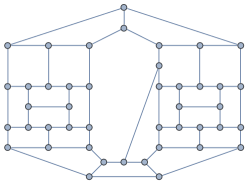
We consider three examples (Fig. 3-5): the Faulkner-Younger graph on 44 vertices, the Thomassen graph on 94 vertices and random graphs. These examples confirm the main principle: a large correlation at a local scale can cause a shift to lower frequencies whereas little correlation implies that the oscillation move transversally and have their bulk continuing to oscillate at frequency λsimilar-toabsent𝜆\sim\lambda. While the notion of ’waves moving transversally’ on a Graph with 44 vertices might seem like a bit of a stretch, the principle remains valid.

2.1. Example 1: Faulkner-Younger Graph

The Faulkner-Younger Graph on 44 vertices is a counterexample [16] (though not the first one) to an old 1880 conjecture of Tait [28]. We compute the global correlation between all pairs of eigenvectors for t𝑡t solving etλ+etμ=1superscript𝑒𝑡𝜆superscript𝑒𝑡𝜇1e^{-t\lambda}+e^{-t\mu}=1 and normalize by dividing by ϕμϕλ2subscriptnormsubscriptitalic-ϕ𝜇subscriptitalic-ϕ𝜆superscript2\|\phi_{\mu}\phi_{\lambda}\|_{\ell^{2}}. Global correlations are clustered around 0.5similar-toabsent0.5\sim 0.5. Notable outliers are

Refer to caption
Figure 3. The Faulkner-Younger Graph on 44 vertices.
  1. (1)

    ϕ12,ϕ15subscriptitalic-ϕ12subscriptitalic-ϕ15\phi_{12},\phi_{15} ( 0.32similar-toabsent0.32\sim 0.32): ϕ12ϕ15subscriptitalic-ϕ12subscriptitalic-ϕ15\phi_{12}\cdot\phi_{15} has 20%percent2020\% of 2limit-fromsuperscript2\ell^{2}-mass on ϕ15subscriptitalic-ϕ15\phi_{15} and 58%percent5858\% of 2limit-fromsuperscript2\ell^{2}-mass on ϕ32subscriptitalic-ϕ32\phi_{32}.

  2. (2)

    ϕ12,ϕ24subscriptitalic-ϕ12subscriptitalic-ϕ24\phi_{12},\phi_{24} ( 0.38similar-toabsent0.38\sim 0.38): ϕ12ϕ24subscriptitalic-ϕ12subscriptitalic-ϕ24\phi_{12}\cdot\phi_{24} has 24%percent2424\% of 2limit-fromsuperscript2\ell^{2}-mass on ϕ26subscriptitalic-ϕ26\phi_{26}, 44%percent4444\% on the highest 6 frequencies.

  3. (3)

    ϕ18,ϕ25subscriptitalic-ϕ18subscriptitalic-ϕ25\phi_{18},\phi_{25} ( 0.7similar-toabsent0.7\sim 0.7): ϕ18ϕ25subscriptitalic-ϕ18subscriptitalic-ϕ25\phi_{18}\cdot\phi_{25} has 60% of 2limit-fromsuperscript2\ell^{2}-mass on the 10 lowest frequencies.

  4. (4)

    ϕ40,ϕ43subscriptitalic-ϕ40subscriptitalic-ϕ43\phi_{40},\phi_{43} ( 0.75similar-toabsent0.75\sim 0.75): ϕ40ϕ43subscriptitalic-ϕ40subscriptitalic-ϕ43\phi_{40}\cdot\phi_{43} has 93% of 2limit-fromsuperscript2\ell^{2}-mass on the 25 lowest frequencies.

  5. (5)

    ϕ42,ϕ44subscriptitalic-ϕ42subscriptitalic-ϕ44\phi_{42},\phi_{44} ( 0.74similar-toabsent0.74\sim 0.74): ϕ42ϕ44subscriptitalic-ϕ42subscriptitalic-ϕ44\phi_{42}\cdot\phi_{44} has 94% of 2limit-fromsuperscript2\ell^{2}-mass on the 25 lowest frequencies.

2.2. Example 2: Thomassen Graph.

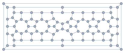
The Thomassen Graph is the smallest cubic planar hypohamiltonian graph in the infinite family constructed by Thomassen [29] to answer a question of Chvátal [9]; we expect eigenvectors to be structured but not arithmetically related.
Refer to caption
Figure 4. The Thomassen Graph on 94 vertices.

We again compute the global correlation between all eigenvectors ϕμ,ϕλsubscriptitalic-ϕ𝜇subscriptitalic-ϕ𝜆\phi_{\mu},\phi_{\lambda} and normalize by dividing by ϕμϕλ2subscriptnormsubscriptitalic-ϕ𝜇subscriptitalic-ϕ𝜆superscript2\|\phi_{\mu}\phi_{\lambda}\|_{\ell^{2}}. Most values at centered around 0.5similar-toabsent0.5\sim 0.5, notable outliers are

  1. (1)

    ϕ10,ϕ15subscriptitalic-ϕ10subscriptitalic-ϕ15\phi_{10},\phi_{15} ( 0.14similar-toabsent0.14\sim 0.14): ϕ10ϕ15subscriptitalic-ϕ10subscriptitalic-ϕ15\phi_{10}\cdot\phi_{15} has 78% of 2limit-fromsuperscript2\ell^{2}-mass on ϕ39subscriptitalic-ϕ39\phi_{39}.

  2. (2)

    ϕ23,ϕ43subscriptitalic-ϕ23subscriptitalic-ϕ43\phi_{23},\phi_{43} ( 0.27similar-toabsent0.27\sim 0.27): ϕ23ϕ43subscriptitalic-ϕ23subscriptitalic-ϕ43\phi_{23}\cdot\phi_{43} has 15%percent1515\% of mass on ϕ43subscriptitalic-ϕ43\phi_{43}, 14%percent1414\% on ϕ90subscriptitalic-ϕ90\phi_{90} and 56%percent5656\% on ϕ91subscriptitalic-ϕ91\phi_{91}.

  3. (3)

    ϕ90,ϕ92subscriptitalic-ϕ90subscriptitalic-ϕ92\phi_{90},\phi_{92} ( 0.75similar-toabsent0.75\sim 0.75): ϕ90ϕ92subscriptitalic-ϕ90subscriptitalic-ϕ92\phi_{90}\cdot\phi_{92} has 76% of 2limit-fromsuperscript2\ell^{2}-mass on the 45 lowest frequencies.

  4. (4)

    ϕ90,ϕ93subscriptitalic-ϕ90subscriptitalic-ϕ93\phi_{90},\phi_{93} ( 0.73similar-toabsent0.73\sim 0.73): ϕ90ϕ93subscriptitalic-ϕ90subscriptitalic-ϕ93\phi_{90}\cdot\phi_{93} has 62% of 2limit-fromsuperscript2\ell^{2}-mass on ϕ40subscriptitalic-ϕ40\phi_{40}.

  5. (5)

    ϕ92,ϕ93subscriptitalic-ϕ92subscriptitalic-ϕ93\phi_{92},\phi_{93} ( 0.93similar-toabsent0.93\sim 0.93): ϕ92ϕ93subscriptitalic-ϕ92subscriptitalic-ϕ93\phi_{92}\cdot\phi_{93} has 57% on ϕ4subscriptitalic-ϕ4\phi_{4}, 26% on ϕ12subscriptitalic-ϕ12\phi_{12} and 12% on ϕ22subscriptitalic-ϕ22\phi_{22}.

These results also indicate an unrelated question: is it common for Graph Laplacians to have two high-frequency eigenvectors whose Hadamard product lies at substantially lower frequencies? A possible explanation would be that very high frequencies can only be obtained by essentially oscillating across every edge: multiplying two such objects would cancel the oscillation. This fails for random/expander graphs so presumably some restriction on the geometry is required.

2.3. Example 3: Random Graphs.

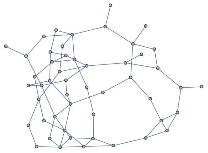
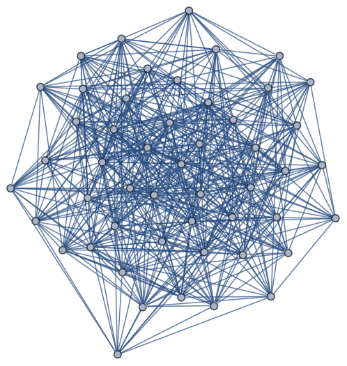
We quickly compare these results to are random graphs. It is easily observed that all the effects weaken and things become more uniform as the number of edges increase: this is not surprising since adding edges turns the graph into a more uniform object whose spectrum is more and more strongly localized.
Refer to caption
Refer to caption
Figure 5. Random Graphs on 50 vertices and 70 edges (left) as well as 500 edges (right).

The typical correlation between any pair of eigenvectors becomes more uniform: in the example in Figure 4 (left), ϕ14ϕ15subscriptitalic-ϕ14subscriptitalic-ϕ15\phi_{14}\cdot\phi_{15} (0.64similar-toabsent0.64\sim 0.64) has 47% of 2limit-fromsuperscript2\ell^{2}-mass on the lowest 10 frequencies. ϕ15ϕ31subscriptitalic-ϕ15subscriptitalic-ϕ31\phi_{15}\cdot\phi_{31} 0.73similar-toabsent0.73\sim 0.73) has 61% on the first 9 frequencies. Moreover, ϕ48ϕ49subscriptitalic-ϕ48subscriptitalic-ϕ49\phi_{48}\cdot\phi_{49} has 41% on ϕ48,ϕ49subscriptitalic-ϕ48subscriptitalic-ϕ49\phi_{48},\phi_{49}. The correlation between eigenvectors of two randomly generated graphs (using Mathematica’s RandomGraph) on 50 vertices and 100 edges has mean 0.48 and standard deviation 0.11. In comparison, for 50 vertices and 1000 edges, the mean correlation is 0.50 with standard deviation 0.01.

3. Proof

3.1. Proof of Theorem 1

Proof.

We phrase the proof in the language of diffusion since it dramatically simplifies notation. ωx(t)subscript𝜔𝑥𝑡\omega_{x}(t) refers to Brownian motion started in x𝑥x at time t𝑡t. The main identity (see e.g. [27]) is the Feynman-Kac formula

[etΔϕλ](x)=𝔼ω(ϕλ(ωx(t))).delimited-[]superscript𝑒𝑡Δsubscriptitalic-ϕ𝜆𝑥subscript𝔼𝜔subscriptitalic-ϕ𝜆subscript𝜔𝑥𝑡\displaystyle\left[e^{t\Delta}\phi_{\lambda}\right](x)=\mathbb{E}_{\omega}(\phi_{\lambda}(\omega_{x}(t))).

Moreover, since Laplacian eigenfunctions diagonalize the heat flow

𝔼ω(ϕλ(ωx(t)))=eλtϕλ(x).subscript𝔼𝜔subscriptitalic-ϕ𝜆subscript𝜔𝑥𝑡superscript𝑒𝜆𝑡subscriptitalic-ϕ𝜆𝑥\mathbb{E}_{\omega}(\phi_{\lambda}(\omega_{x}(t)))=e^{-\lambda t}\phi_{\lambda}(x).

We now start with a series of algebraic manipulations; adding 0 yields

[etΔϕμϕλ](x)ϕλ(x)ϕμ(x)delimited-[]superscript𝑒𝑡Δsubscriptitalic-ϕ𝜇subscriptitalic-ϕ𝜆𝑥subscriptitalic-ϕ𝜆𝑥subscriptitalic-ϕ𝜇𝑥\displaystyle\left[e^{t\Delta}\phi_{\mu}\phi_{\lambda}\right](x)-\phi_{\lambda}(x)\phi_{\mu}(x) =[etΔϕμϕλ](x)ϕλ(x)[etΔϕμ](x)absentdelimited-[]superscript𝑒𝑡Δsubscriptitalic-ϕ𝜇subscriptitalic-ϕ𝜆𝑥subscriptitalic-ϕ𝜆𝑥delimited-[]superscript𝑒𝑡Δsubscriptitalic-ϕ𝜇𝑥\displaystyle=\left[e^{t\Delta}\phi_{\mu}\phi_{\lambda}\right](x)-\phi_{\lambda}(x)\left[e^{t\Delta}\phi_{\mu}\right](x)
+ϕλ(x)[etΔϕμ](x)ϕλ(x)ϕμ(x).subscriptitalic-ϕ𝜆𝑥delimited-[]superscript𝑒𝑡Δsubscriptitalic-ϕ𝜇𝑥subscriptitalic-ϕ𝜆𝑥subscriptitalic-ϕ𝜇𝑥\displaystyle+\phi_{\lambda}(x)\left[e^{t\Delta}\phi_{\mu}\right](x)-\phi_{\lambda}(x)\phi_{\mu}(x).

This can be rewritten as

[etΔϕμϕλ](x)ϕλ(x)ϕμ(x)delimited-[]superscript𝑒𝑡Δsubscriptitalic-ϕ𝜇subscriptitalic-ϕ𝜆𝑥subscriptitalic-ϕ𝜆𝑥subscriptitalic-ϕ𝜇𝑥\displaystyle\left[e^{t\Delta}\phi_{\mu}\phi_{\lambda}\right](x)-\phi_{\lambda}(x)\phi_{\mu}(x) =𝔼x(ϕλ(ωx(t))ϕμ(ωx(t)))𝔼x(ϕλ(x)ϕμ(ωx(t)))absentsubscript𝔼𝑥subscriptitalic-ϕ𝜆subscript𝜔𝑥𝑡subscriptitalic-ϕ𝜇subscript𝜔𝑥𝑡subscript𝔼𝑥subscriptitalic-ϕ𝜆𝑥subscriptitalic-ϕ𝜇subscript𝜔𝑥𝑡\displaystyle=\mathbb{E}_{x}\left(\phi_{\lambda}(\omega_{x}(t))\phi_{\mu}(\omega_{x}(t))\right)-\mathbb{E}_{x}\left(\phi_{\lambda}(x)\phi_{\mu}(\omega_{x}(t))\right)
+𝔼x(ϕλ(x)ϕμ(ωx(t)))ϕλ(x)ϕμ(x)subscript𝔼𝑥subscriptitalic-ϕ𝜆𝑥subscriptitalic-ϕ𝜇subscript𝜔𝑥𝑡subscriptitalic-ϕ𝜆𝑥subscriptitalic-ϕ𝜇𝑥\displaystyle+\mathbb{E}_{x}\left(\phi_{\lambda}(x)\phi_{\mu}(\omega_{x}(t))\right)-\phi_{\lambda}(x)\phi_{\mu}(x)

Using linearity of expectation

𝔼x(ϕλ(ωx(t))ϕμ(ωx(t)))𝔼x(ϕλ(x)ϕμ(ωx(t)))=𝔼x(ϕμ(ωx(t))(ϕλ(ωx(t))ϕλ(x)))subscript𝔼𝑥subscriptitalic-ϕ𝜆subscript𝜔𝑥𝑡subscriptitalic-ϕ𝜇subscript𝜔𝑥𝑡subscript𝔼𝑥subscriptitalic-ϕ𝜆𝑥subscriptitalic-ϕ𝜇subscript𝜔𝑥𝑡subscript𝔼𝑥subscriptitalic-ϕ𝜇subscript𝜔𝑥𝑡subscriptitalic-ϕ𝜆subscript𝜔𝑥𝑡subscriptitalic-ϕ𝜆𝑥\mathbb{E}_{x}\left(\phi_{\lambda}(\omega_{x}(t))\phi_{\mu}(\omega_{x}(t))\right)-\mathbb{E}_{x}\left(\phi_{\lambda}(x)\phi_{\mu}(\omega_{x}(t))\right)=\mathbb{E}_{x}\left(\phi_{\mu}(\omega_{x}(t))\left(\phi_{\lambda}(\omega_{x}(t))-\phi_{\lambda}(x)\right)\right)

and

𝔼x(ϕλ(x)ϕμ(ωx(t)))ϕλ(x)ϕμ(x)=ϕλ(x)𝔼x(ϕμ(ωx(t))ϕμ(x)).subscript𝔼𝑥subscriptitalic-ϕ𝜆𝑥subscriptitalic-ϕ𝜇subscript𝜔𝑥𝑡subscriptitalic-ϕ𝜆𝑥subscriptitalic-ϕ𝜇𝑥subscriptitalic-ϕ𝜆𝑥subscript𝔼𝑥subscriptitalic-ϕ𝜇subscript𝜔𝑥𝑡subscriptitalic-ϕ𝜇𝑥\mathbb{E}_{x}\left(\phi_{\lambda}(x)\phi_{\mu}(\omega_{x}(t))\right)-\phi_{\lambda}(x)\phi_{\mu}(x)=\phi_{\lambda}(x)\mathbb{E}_{x}\left(\phi_{\mu}(\omega_{x}(t))-\phi_{\mu}(x)\right).

Writing ϕμ(ωx(t))=ϕμ(ωx(t))ϕμ(x)+ϕμ(x)subscriptitalic-ϕ𝜇subscript𝜔𝑥𝑡subscriptitalic-ϕ𝜇subscript𝜔𝑥𝑡subscriptitalic-ϕ𝜇𝑥subscriptitalic-ϕ𝜇𝑥\phi_{\mu}(\omega_{x}(t))=\phi_{\mu}(\omega_{x}(t))-\phi_{\mu}(x)+\phi_{\mu}(x) and plugging into the first term yields

[etΔϕμϕλ](x)ϕλ(x)ϕμ(x)delimited-[]superscript𝑒𝑡Δsubscriptitalic-ϕ𝜇subscriptitalic-ϕ𝜆𝑥subscriptitalic-ϕ𝜆𝑥subscriptitalic-ϕ𝜇𝑥\displaystyle\left[e^{t\Delta}\phi_{\mu}\phi_{\lambda}\right](x)-\phi_{\lambda}(x)\phi_{\mu}(x) =ϕλ(x)𝔼x(ϕμ(ωx(t))ϕμ(x))absentsubscriptitalic-ϕ𝜆𝑥subscript𝔼𝑥subscriptitalic-ϕ𝜇subscript𝜔𝑥𝑡subscriptitalic-ϕ𝜇𝑥\displaystyle=\phi_{\lambda}(x)\mathbb{E}_{x}\left(\phi_{\mu}(\omega_{x}(t))-\phi_{\mu}(x)\right)
+ϕμ(x)𝔼x(ϕλ(ωx(t))ϕλ(x))subscriptitalic-ϕ𝜇𝑥subscript𝔼𝑥subscriptitalic-ϕ𝜆subscript𝜔𝑥𝑡subscriptitalic-ϕ𝜆𝑥\displaystyle+\phi_{\mu}(x)\mathbb{E}_{x}\left(\phi_{\lambda}(\omega_{x}(t))-\phi_{\lambda}(x)\right)
+𝔼x((ϕμ(ωx(t))ϕμ(x))(ϕλ(ωx(t))ϕλ(x))).subscript𝔼𝑥subscriptitalic-ϕ𝜇subscript𝜔𝑥𝑡subscriptitalic-ϕ𝜇𝑥subscriptitalic-ϕ𝜆subscript𝜔𝑥𝑡subscriptitalic-ϕ𝜆𝑥\displaystyle+\mathbb{E}_{x}\left((\phi_{\mu}(\omega_{x}(t))-\phi_{\mu}(x))(\phi_{\lambda}(\omega_{x}(t))-\phi_{\lambda}(x))\right).

However, two out of three of these expectations can be explicitly computed and this yields

[etΔϕμϕλ](x)ϕλ(x)ϕμ(x)delimited-[]superscript𝑒𝑡Δsubscriptitalic-ϕ𝜇subscriptitalic-ϕ𝜆𝑥subscriptitalic-ϕ𝜆𝑥subscriptitalic-ϕ𝜇𝑥\displaystyle\left[e^{t\Delta}\phi_{\mu}\phi_{\lambda}\right](x)-\phi_{\lambda}(x)\phi_{\mu}(x) =ϕλ(x)(eμt1)ϕμ(x)absentsubscriptitalic-ϕ𝜆𝑥superscript𝑒𝜇𝑡1subscriptitalic-ϕ𝜇𝑥\displaystyle=\phi_{\lambda}(x)(e^{-\mu t}-1)\phi_{\mu}(x)
+ϕμ(x)(eλt1)ϕλ(x)subscriptitalic-ϕ𝜇𝑥superscript𝑒𝜆𝑡1subscriptitalic-ϕ𝜆𝑥\displaystyle+\phi_{\mu}(x)(e^{-\lambda t}-1)\phi_{\lambda}(x)
+𝔼x((ϕμ(ωx(t))ϕμ(x))(ϕλ(ωx(t))ϕλ(x))).subscript𝔼𝑥subscriptitalic-ϕ𝜇subscript𝜔𝑥𝑡subscriptitalic-ϕ𝜇𝑥subscriptitalic-ϕ𝜆subscript𝜔𝑥𝑡subscriptitalic-ϕ𝜆𝑥\displaystyle+\mathbb{E}_{x}\left((\phi_{\mu}(\omega_{x}(t))-\phi_{\mu}(x))(\phi_{\lambda}(\omega_{x}(t))-\phi_{\lambda}(x))\right).

At the same time, the expectation can be rewritten in terms of the heat kernel as

𝔼x((ϕμ(ωx(t))ϕμ(x))(ϕλ(ωx(t))ϕλ(x)))=Ωp(t,x,y)(ϕλ(y)ϕλ(x))(ϕμ(y)ϕμ(x))𝑑y.subscript𝔼𝑥subscriptitalic-ϕ𝜇subscript𝜔𝑥𝑡subscriptitalic-ϕ𝜇𝑥subscriptitalic-ϕ𝜆subscript𝜔𝑥𝑡subscriptitalic-ϕ𝜆𝑥subscriptΩ𝑝𝑡𝑥𝑦subscriptitalic-ϕ𝜆𝑦subscriptitalic-ϕ𝜆𝑥subscriptitalic-ϕ𝜇𝑦subscriptitalic-ϕ𝜇𝑥differential-d𝑦\mathbb{E}_{x}\left((\phi_{\mu}(\omega_{x}(t))-\phi_{\mu}(x))(\phi_{\lambda}(\omega_{x}(t))-\phi_{\lambda}(x))\right)=\int_{\Omega}{p(t,x,y)(\phi_{\lambda}(y)-\phi_{\lambda}(x))(\phi_{\mu}(y)-\phi_{\mu}(x))dy}.

Summarizing, we obtain the fundamental identity

[etΔϕμϕλ](x)delimited-[]superscript𝑒𝑡Δsubscriptitalic-ϕ𝜇subscriptitalic-ϕ𝜆𝑥\displaystyle\left[e^{t\Delta}\phi_{\mu}\phi_{\lambda}\right](x) =(eλt+eμt1)ϕλ(x)ϕμ(x)absentsuperscript𝑒𝜆𝑡superscript𝑒𝜇𝑡1subscriptitalic-ϕ𝜆𝑥subscriptitalic-ϕ𝜇𝑥\displaystyle=\left(e^{-\lambda t}+e^{-\mu t}-1\right)\phi_{\lambda}(x)\phi_{\mu}(x)
+Ωp(t,x,y)(ϕλ(y)ϕλ(x))(ϕμ(y)ϕμ(x))𝑑y.subscriptΩ𝑝𝑡𝑥𝑦subscriptitalic-ϕ𝜆𝑦subscriptitalic-ϕ𝜆𝑥subscriptitalic-ϕ𝜇𝑦subscriptitalic-ϕ𝜇𝑥differential-d𝑦\displaystyle+\int_{\Omega}{p(t,x,y)(\phi_{\lambda}(y)-\phi_{\lambda}(x))(\phi_{\mu}(y)-\phi_{\mu}(x))dy}.

It remains to determine the size of t𝑡t such that

eλt+eμt=1.superscript𝑒𝜆𝑡superscript𝑒𝜇𝑡1e^{-\lambda t}+e^{-\mu t}=1.

It is clear that the left-hand side is bigger than 1 for t𝑡t sufficiently small. Setting t=αlog(eλ/μ)λ1𝑡𝛼𝑒𝜆𝜇superscript𝜆1t=\alpha\log{(e\lambda/\mu)}\lambda^{-1} shows that

eλt+eμt=(eμλ)α+(eμλ)αμλ.superscript𝑒𝜆𝑡superscript𝑒𝜇𝑡superscript𝑒𝜇𝜆𝛼superscript𝑒𝜇𝜆𝛼𝜇𝜆e^{-\lambda t}+e^{-\mu t}=\left(\frac{e\mu}{\lambda}\right)^{\alpha}+\left(\frac{e\mu}{\lambda}\right)^{\alpha\frac{\mu}{\lambda}}.

A computation shows that (ex)0.8+(ex)0.8x1superscript𝑒𝑥0.8superscript𝑒𝑥0.8𝑥1(ex)^{0.8}+(ex)^{0.8x}\geq 1 on (0,e)0𝑒(0,e). This shows that the solution tsuperscript𝑡t^{*} satisfies

t0.8log(eλ/μ)λ1.superscript𝑡0.8𝑒𝜆𝜇superscript𝜆1t^{*}\geq 0.8\log{(e\lambda/\mu)}\lambda^{-1}.

Simultaneously, (ex)1+(ex)x<1superscript𝑒𝑥1superscript𝑒𝑥𝑥1(ex)^{1}+(ex)^{x}<1 on (0,0.02)00.02(0,0.02), which shows

tlog(eλ/μ)λ1forμλ50.formulae-sequencesuperscript𝑡𝑒𝜆𝜇superscript𝜆1for𝜇𝜆50t^{*}\leq\log{(e\lambda/\mu)}\lambda^{-1}\qquad\mbox{for}\qquad\mu\leq\frac{\lambda}{50}.

If μλ/50𝜇𝜆50\mu\geq\lambda/50, then

eλt+eμteλt+eλt/50<1for some t2.8822λ3log(eλμ)λ1formulae-sequencesuperscript𝑒𝜆𝑡superscript𝑒𝜇𝑡superscript𝑒𝜆𝑡superscript𝑒𝜆𝑡501similar-tofor some 𝑡2.8822𝜆3𝑒𝜆𝜇superscript𝜆1e^{-\lambda t}+e^{-\mu t}\leq e^{-\lambda t}+e^{-\lambda t/50}<1\qquad\mbox{for some }~{}t\sim\frac{2.8822}{\lambda}\leq 3\log{\left(\frac{e\lambda}{\mu}\right)}\lambda^{-1}

which shows

0.8log(eλμ)λ1t3log(eλμ)λ1.0.8𝑒𝜆𝜇superscript𝜆1superscript𝑡3𝑒𝜆𝜇superscript𝜆10.8\log{\left(\frac{e\lambda}{\mu}\right)}\lambda^{-1}\leq t^{*}\leq 3\log{\left(\frac{e\lambda}{\mu}\right)}\lambda^{-1}.

This shows the desired result, the case of Graph Laplacians is completely identical. ∎

3.2. Proof of the Corollaries

Proof.

Let us assume the statement fails and product ϕμϕλsubscriptitalic-ϕ𝜇subscriptitalic-ϕ𝜆\phi_{\mu}\phi_{\lambda} has a large portion of its L2limit-fromsuperscript𝐿2L^{2}-energy at frequencies λ/log(eλ/μ)absent𝜆𝑒𝜆𝜇\leq\lambda/\log{(e\lambda/\mu)}

λkλ/log(eλ/μ)|ϕμϕλ,ϕk|2δ2ϕμϕλL22.subscriptsubscript𝜆𝑘𝜆𝑒𝜆𝜇superscriptsubscriptitalic-ϕ𝜇subscriptitalic-ϕ𝜆subscriptitalic-ϕ𝑘2superscript𝛿2subscriptsuperscriptnormsubscriptitalic-ϕ𝜇subscriptitalic-ϕ𝜆2superscript𝐿2\sum_{\lambda_{k}\leq\lambda/\log{(e\lambda/\mu)}}{|\left\langle\phi_{\mu}\phi_{\lambda},\phi_{k}\right\rangle|^{2}}\geq\delta^{2}\|\phi_{\mu}\phi_{\lambda}\|^{2}_{L^{2}}.

Then, clearly,

etΔ(ϕμϕλ)L22=k=0e2λkt|ϕμϕλ,ϕk|2λkλ/log(eλ/μ)e2λkt|ϕμϕλ,ϕk|2.superscriptsubscriptnormsuperscript𝑒𝑡Δsubscriptitalic-ϕ𝜇subscriptitalic-ϕ𝜆superscript𝐿22superscriptsubscript𝑘0superscript𝑒2subscript𝜆𝑘𝑡superscriptsubscriptitalic-ϕ𝜇subscriptitalic-ϕ𝜆subscriptitalic-ϕ𝑘2superscriptsubscriptsubscript𝜆𝑘𝜆𝑒𝜆𝜇superscript𝑒2subscript𝜆𝑘𝑡superscriptsubscriptitalic-ϕ𝜇subscriptitalic-ϕ𝜆subscriptitalic-ϕ𝑘2\|e^{t\Delta}(\phi_{\mu}\phi_{\lambda})\|_{L^{2}}^{2}=\sum_{k=0}^{\infty}{e^{-2\lambda_{k}t}|\left\langle\phi_{\mu}\phi_{\lambda},\phi_{k}\right\rangle|^{2}}\geq\sum_{\lambda_{k}\leq\lambda/\log{(e\lambda/\mu)}}^{\infty}{e^{-2\lambda_{k}t}|\left\langle\phi_{\mu}\phi_{\lambda},\phi_{k}\right\rangle|^{2}}.

For tlog(eλ/μ)λ1similar-to𝑡𝑒𝜆𝜇superscript𝜆1t\sim\log{(e\lambda/\mu)}\lambda^{-1}, we see that these exponential factors are roughly 1similar-toabsent1\sim 1 and thus

etΔ(ϕμϕλ)L22e2δ2ϕμϕλL22,superscriptsubscriptnormsuperscript𝑒𝑡Δsubscriptitalic-ϕ𝜇subscriptitalic-ϕ𝜆superscript𝐿22superscript𝑒2superscript𝛿2subscriptsuperscriptnormsubscriptitalic-ϕ𝜇subscriptitalic-ϕ𝜆2superscript𝐿2\|e^{t\Delta}(\phi_{\mu}\phi_{\lambda})\|_{L^{2}}^{2}\geq e^{-2}\delta^{2}\|\phi_{\mu}\phi_{\lambda}\|^{2}_{L^{2}},

which then implies the desired result since heat evolution and local correlation coincide for that value of t𝑡t. The proof of Corollary 2 follows the same lines: assume that for tlog(eλ/μ)λ1similar-to𝑡𝑒𝜆𝜇superscript𝜆1t\sim\log{(e\lambda/\mu)}\lambda^{-1}

Mp(t,x,y)(ϕλ(y)ϕλ(x))(ϕμ(y)ϕμ(x))𝑑yLx2δϕμϕλL2.subscriptnormsubscript𝑀𝑝𝑡𝑥𝑦subscriptitalic-ϕ𝜆𝑦subscriptitalic-ϕ𝜆𝑥subscriptitalic-ϕ𝜇𝑦subscriptitalic-ϕ𝜇𝑥differential-d𝑦subscriptsuperscript𝐿2𝑥𝛿subscriptnormsubscriptitalic-ϕ𝜇subscriptitalic-ϕ𝜆superscript𝐿2\left\|\int_{M}{p(t,x,y)(\phi_{\lambda}(y)-\phi_{\lambda}(x))(\phi_{\mu}(y)-\phi_{\mu}(x))dy}\right\|_{L^{2}_{x}}\geq\delta\|\phi_{\mu}\phi_{\lambda}\|_{L^{2}}.

The main result implies

Ωp(t,x,y)(ϕλ(y)ϕλ(x))(ϕμ(y)ϕμ(x))𝑑yLx22=etΔ(ϕμϕλ)L22.superscriptsubscriptnormsubscriptΩ𝑝𝑡𝑥𝑦subscriptitalic-ϕ𝜆𝑦subscriptitalic-ϕ𝜆𝑥subscriptitalic-ϕ𝜇𝑦subscriptitalic-ϕ𝜇𝑥differential-d𝑦subscriptsuperscript𝐿2𝑥2superscriptsubscriptnormsuperscript𝑒𝑡Δsubscriptitalic-ϕ𝜇subscriptitalic-ϕ𝜆superscript𝐿22\left\|\int_{\Omega}{p(t,x,y)(\phi_{\lambda}(y)-\phi_{\lambda}(x))(\phi_{\mu}(y)-\phi_{\mu}(x))dy}\right\|_{L^{2}_{x}}^{2}=\|e^{t\Delta}(\phi_{\mu}\phi_{\lambda})\|_{L^{2}}^{2}.

At the same time, we can write

δ2ϕμϕλL22etΔ(ϕμϕλ)L22superscript𝛿2superscriptsubscriptnormsubscriptitalic-ϕ𝜇subscriptitalic-ϕ𝜆superscript𝐿22superscriptsubscriptnormsuperscript𝑒𝑡Δsubscriptitalic-ϕ𝜇subscriptitalic-ϕ𝜆superscript𝐿22\displaystyle\delta^{2}\|\phi_{\mu}\phi_{\lambda}\|_{L^{2}}^{2}\leq\|e^{t\Delta}(\phi_{\mu}\phi_{\lambda})\|_{L^{2}}^{2} =k=1e2λkt|ϕμϕλ,ϕk|2absentsuperscriptsubscript𝑘1superscript𝑒2subscript𝜆𝑘𝑡superscriptsubscriptitalic-ϕ𝜇subscriptitalic-ϕ𝜆subscriptitalic-ϕ𝑘2\displaystyle=\sum_{k=1}^{\infty}{e^{-2\lambda_{k}t}|\left\langle\phi_{\mu}\phi_{\lambda},\phi_{k}\right\rangle|^{2}}
λkcλ|ϕμϕλ,ϕk|2+λkcλe2cλkt|ϕμϕλ,ϕk|2absentsuperscriptsubscriptsubscript𝜆𝑘𝑐𝜆superscriptsubscriptitalic-ϕ𝜇subscriptitalic-ϕ𝜆subscriptitalic-ϕ𝑘2superscriptsubscriptsubscript𝜆𝑘𝑐𝜆superscript𝑒2𝑐subscript𝜆𝑘𝑡superscriptsubscriptitalic-ϕ𝜇subscriptitalic-ϕ𝜆subscriptitalic-ϕ𝑘2\displaystyle\leq\sum_{\lambda_{k}\leq c\lambda}^{\infty}{|\left\langle\phi_{\mu}\phi_{\lambda},\phi_{k}\right\rangle|^{2}}+\sum_{\lambda_{k}\geq c\lambda}^{\infty}{e^{-2c\lambda_{k}t}|\left\langle\phi_{\mu}\phi_{\lambda},\phi_{k}\right\rangle|^{2}}
λkcλ|ϕμϕλ,ϕk|2+e2cλkcλ|ϕμϕλ,ϕk|2.absentsuperscriptsubscriptsubscript𝜆𝑘𝑐𝜆superscriptsubscriptitalic-ϕ𝜇subscriptitalic-ϕ𝜆subscriptitalic-ϕ𝑘2superscript𝑒2𝑐superscriptsubscriptsubscript𝜆𝑘𝑐𝜆superscriptsubscriptitalic-ϕ𝜇subscriptitalic-ϕ𝜆subscriptitalic-ϕ𝑘2\displaystyle\leq\sum_{\lambda_{k}\leq c\lambda}^{\infty}{|\left\langle\phi_{\mu}\phi_{\lambda},\phi_{k}\right\rangle|^{2}}+e^{-2c}\sum_{\lambda_{k}\geq c\lambda}^{\infty}{|\left\langle\phi_{\mu}\phi_{\lambda},\phi_{k}\right\rangle|^{2}}.

This then implies

λkcλ|ϕμϕλ,ϕk|2δ2e2c1e2c1.superscriptsubscriptsubscript𝜆𝑘𝑐𝜆superscriptsubscriptitalic-ϕ𝜇subscriptitalic-ϕ𝜆subscriptitalic-ϕ𝑘2superscript𝛿2superscript𝑒2𝑐1superscript𝑒2𝑐1\sum_{\lambda_{k}\leq c\lambda}^{\infty}{|\left\langle\phi_{\mu}\phi_{\lambda},\phi_{k}\right\rangle|^{2}}\geq\frac{\delta^{2}e^{2c}-1}{e^{2c}-1}.

The estimate is nontrivial for clog(1/δ)similar-to𝑐1𝛿c\sim\log{(1/\delta)} in which case the right-hand side is δ2.similar-toabsentsuperscript𝛿2\sim\delta^{2}.

4. Remarks

We believe that the local correlation

Mp(t,x,y)(ϕλ(y)ϕλ(x))(ϕμ(y)ϕμ(x))𝑑ysubscript𝑀𝑝𝑡𝑥𝑦subscriptitalic-ϕ𝜆𝑦subscriptitalic-ϕ𝜆𝑥subscriptitalic-ϕ𝜇𝑦subscriptitalic-ϕ𝜇𝑥differential-d𝑦\int_{M}{p(t,x,y)(\phi_{\lambda}(y)-\phi_{\lambda}(x))(\phi_{\mu}(y)-\phi_{\mu}(x))dy}

is of intrinsic interest for possibly other reasons as well. Note that the eigenfunctions sin(5x)5𝑥\sin{(5x)} and sin(3x)sin(4y)3𝑥4𝑦\sin{(3x)}\sin{(4y)} on 𝕋2superscript𝕋2\mathbb{T}^{2} have the same eigenvalue but behave very differently from each other. Conversely, sin(5x)5𝑥\sin{(5x)} and sin(4x)4𝑥\sin{(4x)} correspond to different eigenvalues but are somehow ’more’ similar. This question has tremendous importance in applications and was addressed by Coifman in various collaborations [10, 11, 12, 13] and was the subject of the Ph.D. theses of Jerrod Ankenmann [1], Sarah Constantin [15] and William Leeb [20] as well as additional work of Leeb [21] and Ankenmann & Leeb [2]. A crucial ingredient is to measure similarity of eigenfunctions by looking at inner products restricted to a subset of the manifold. Considering L2limit-fromsuperscript𝐿2L^{2}-normalized eigenfunctions einθ/2πsuperscript𝑒𝑖𝑛𝜃2𝜋e^{in\theta}/\sqrt{2\pi}, we see that

|abei(nn)𝑑θ|=1|nn||22cos(nn)(ba)|,superscriptsubscript𝑎𝑏superscript𝑒𝑖𝑛superscript𝑛differential-d𝜃1𝑛superscript𝑛22𝑛superscript𝑛𝑏𝑎\left|\int_{a}^{b}{e^{i(n-n^{\prime})}d\theta}\right|=\frac{1}{|n-n^{\prime}|}\left|2-2\cos{(n-n^{\prime})(b-a)}\right|,

which is a quantity that does not depend on a,b𝑎𝑏a,b but merely on the scale |ba|𝑏𝑎|b-a|. The Ph.D. thesis of Constantin [15] contains a particularly nice example where 𝕊3superscript𝕊3\mathbb{S}^{3} is equipped with two different metrics leading to a different affinity between the eigenfunctions (that coincide in both). We note that this idea of local testing is very similar to our global correlation functional. This raises the question whether the global correlation could be used as an affinity measure in applications.

Acknowledgments. The author was asked how ϕμϕλ,ϕνsubscriptitalic-ϕ𝜇subscriptitalic-ϕ𝜆subscriptitalic-ϕ𝜈\left\langle\phi_{\mu}\phi_{\lambda},\phi_{\nu}\right\rangle behaves independently by Martin Ehler during the workshop ’Tractability of High Dimensional Problems and Discrepancy’ hosted by the Erwin Schrödinger Institute (ESI) in Vienna from 25.-29.Sep. 2017 and by Michael Bronstein, Frederico Monti & Emanuele Rodola during a visit at Yale in Nov 2017 and their questions inspired this paper. The author is also grateful to Raphy Coifman for many discussions about the dual geometry induced by eigenfunctions.

References

  • [1] J. Ankenmann, Geometry and Analysis of Dual Networks on Questionnaires, PhD thesis, Yale, 2014
  • [2] J. Ankenmann and W. Leeb, Mixed Hölder matrix discovery via wavelet shrinkage and Calderon–Zygmund decompositions, to appear in Appl. Comp. Harm. Anal.
  • [3] ] J. Bernstein and A. Reznikoff, Analytic continuation of representations and estimates of automorphic forms, Ann. of Math. 150 (1999), 329–352.
  • [4] M. Berry, Regular and irregular semiclassical wavefunctions. J. Phys. A 10 (1977), no. 12, 2083–2091
  • [5] M. Blair, H. Smith and C. Sogge, On multilinear spectral cluster estimates for manifolds with boundary. Math. Res. Lett. 15 (2008), no. 3, 419–426.
  • [6] N. Burq, P. Gérard and N. Tzvetkov, Bilinear eigenfunction estimates and the nonlinear Schrödinger equation on surfaces. Invent. Math. 159 (2005), no. 1, 187–223.
  • [7] N. Burq, P. Gérard and N. Tzvetkov, Multilinear estimates for the Laplace spectral projectors on compact manifolds. C. R. Math. Acad. Sci. Paris 338 (2004), no. 5, 359–364.
  • [8] F. R. Chung, Spectral graph theory. CBMS Regional Conference Series in Mathematics, 92. Published for the Conference Board of the Mathematical Sciences, Washington, DC; by the American Mathematical Society, Providence, RI, 1997.
  • [9] V. Chvátal: Flip-flops in hypohamiltonian graphs. Can. Math. Bull. 16, 33–41. (1973)
  • [10] R. Coifman and M. Gavish, Harmonic analysis of digital data bases. in:Wavelets and multiscale analysis, 161–197, Appl. Numer. Harmon. Anal., Birkhäuser/Springer, New York, 2011.
  • [11] R. Coifman and M. Gavish, Sampling, denoising and compression of matrices by coherent matrix organization. Appl. Comput. Harmon. Anal. 33 (2012), no. 3, 354–369.
  • [12] R. Coifman and M. Gavish, Harmonic analysis of databases and matrices. Excursions in harmonic analysis. Volume 1, 297–310, Appl. Numer. Harmon. Anal., Birkhäuser/Springer, New York, 2013.
  • [13] R. Coifman and M. Gavish, Information integration, organization, and numerical harmonic analysis. Mathematical and computational modeling, 254–271, Pure Appl. Math. (Hoboken), Wiley, Hoboken, NJ, 2015.
  • [14] R. Coifman and W. Leeb. Hölder-Lipschitz norms and their duals on spaces with semigroups, with applications to Earth Mover’s Distance. Journal of Fourier Analysis and Applications, 22(4) (2016) 910–953.
  • [15] S. Constantin, Diffusion Harmonics and Dual Geometry on Carnot Manifolds, PhD thesis, Yale, 2015.
  • [16] G. B. Faulkner and D. H. Younger, Non-Hamiltonian Cubic Planar Maps. Discr. Math. 7, 67–74, 1974.
  • [17] F. Filbir, H. Mhaskar, H. Marcinkiewicz-Zygmund measures on manifolds. J. Complexity 27 (2011), no. 6, 568–596.
  • [18] D. Hejhal and B. Rackner, On the topography of Maass waveforms for PSL(2,Z). Experiment. Math. 1 (1992), no. 4, 275–305.
  • [19] B. Krötz and R. Stanton, Holomorphic extension of representations: (I) automorphic functions, Ann. of Math. 159 (2004)
  • [20] W. Leeb, Topics in Metric Approximation, Ph.D. thesis, Yale, 2015
  • [21] W. Leeb, The mixed Lipschitz space and its dual for tree metrics, to appear in Appl. Comp. Harm. Anal.
  • [22] O. Litany, E. Rodola, A. M. Bronstein, M. M. Bronstein, Fully spectral partial shape matching, Computer Graphics Forum, Vol. 36(2), 2017.
  • [23] G. Mishne, R. Talmon, R. Meir, J. Schiller, M. Lavzin, U. Dubin and R. Coifman, Hierarchical Coupled Geometry Analysis for Neuronal Structure and Activity Pattern Discovery, IEEE Journal of Selected Topics in Signal Processing 10 (7), 1238–1253
  • [24] H.N. Mhaskar, A generalized diffusion frame for parsimonious representation of functions on data defined manifolds, Neural Networks 24 (2011) 345–359.
  • [25] H. N. Mhaskar, Eignets for function approximation on manifolds. Appl. Comput. Harmon. Anal. 29 (2010), no. 1, 63–87.
  • [26] P. Sarnak, Integrals of products of eigenfunctions. Internat. Math. Res. Notices 1994, no. 6, 251ff.
  • [27] S. Steinerberger, Lower bounds on nodal sets of eigenfunctions via the heat flow, Communications in Partial Differential Equations 39, 2240–2261 (2014)
  • [28] P. G. Tait, P. G. Remarks on the Colouring of Maps. Proc. Royal Soc. Edinburgh 10, 729, 1880.
  • [29] C. Thomassen, C.: Planar cubic hypohamiltonian and hypotraceable graphs. J. Comb. Theory B 30, 36–44. (1981)