MULTIPLE IMPROVEMENTS OF

MULTIPLE IMPUTATION LIKELIHOOD RATIO TESTS

Kin Wai Chan¹ and Xiao-Li Meng²

Department of Statistics, The Chinese University of Hong Kong¹

Department of Statistics, Harvard University²

Abstract: Multiple imputation (MI) inference handles missing data by imputing the missing values $m$ times, and then combining the results from the $m$ complete-data analyses. However, the existing method for combining likelihood ratio tests (LRTs) has multiple defects: (i) the combined test statistic can be negative, but its null distribution is approximated by an $F$-distribution; (ii) it is not invariant to re-parametrization; (iii) it fails to ensure monotonic power owing to its use of an inconsistent estimator of the fraction of missing information (FMI) under the alternative hypothesis; and (iv) it requires nontrivial access to the LRT statistic as a function of parameters instead of data sets. We show, using both theoretical derivations and empirical investigations, that essentially all of these problems can be straightforwardly addressed if we are willing to perform an additional LRT by stacking the $m$ completed data sets as one big completed data set. This enables users to implement the MI LRT without modifying the complete-data procedure. A particularly intriguing finding is that the FMI can be estimated consistently by an LRT statistic for testing whether the $m$ completed data sets can be regarded effectively as samples coming from a common model. Practical guidelines are provided based on an extensive comparison of existing MI tests. Issues related to nuisance parameters are also discussed.

Key words and phrases: Fraction of missing information, missing data, invariant test, monotonic power, robust estimation.

1 Historical Successes and Failures

1.1 The Need for Multiple Imputation Likelihood-Ratio Tests

Missing-data problems are ubiquitous in practice, to the extent that the absence of any missingness is often a strong indication that the data have been pre-processed or manipulated in some way (e.g., Blocker and Meng, 2013). Multiple imputation (MI) (Rubin, 1978, 2004) has been a preferred method, especially by those who are ill-equipped to handle missingness on their own, owing to a lack of information or skills or resources. MI relies on the data collector (e.g., a census bureau) building a reliable imputation model to fill in the missing data $m(\geq 2)$ times. In this way, users can apply their preferred software or procedures designed for complete data, and do so $m$ times. MI inference is then performed by appropriately combining these $m$ complete-data results. Note that in a typical analysis of public MI data, the analyst has no control over or understanding of how the imputation was done, including the choice of the model and $m$, which is often small in reality (e.g., $3\leq m\leq 10$). The analyst’s job is to analyze the given $m$ completed data sets as appropriately as possible, but only using complete-data procedures or software routines.

Although MI was designed initially for public-use data sets, over the years, it has become a method of choice in general, because it separates handling the missingness from the analysis (e.g., Tu et al., 1993; Rubin, 1996, 2004; Schafer, 1999; King et al., 2001; Peugh and Enders, 2004; Kenward and Carpenter, 2007; Rose and Fraser, 2008; Holan et al., 2010; Kim and Yang, 2017). Software routines for performing MI are now available in R (Su et al., 2011), Stata (Royston and White, 2011), SAS (Berglund and Heeringa, 2014), and SPSS; see Harel and Zhou (2007) and Horton and Kleinman (2007) for summaries.

This convenient separation, however, creates an issue of uncongeniality, that is, an incompatibility between the imputation model and the subsequent analysis procedures (Meng, 1994a). This issue is examined in detail by Xie and Meng (2017), who show that uncongeniality is easiest to deal with when the imputer’s model is more saturated than the user’s model/procedure, and when the user is conducting an efficient analysis, such as a likelihood inference. Therefore, this study focuses on conducting MI likelihood ratio tests (LRTs), assuming the imputation model is sufficiently saturated to render the common assumptions made in the literature about conducting LRTs with MI valid.

Like many hypothesis testing procedures in common practice, the exact null distributions of various MI test statistics, LRTs or not, are intractable. This intractability is not computational, but rather statistical, owing to the well-known issue of a nuisance parameter, that is, the lack of a pivotal quantity, as highlighted by the Behrens–Fisher problem (Wallace, 1980). Indeed, the nuisance parameter in the MI context is the so-called “fraction of missing information” (FMI), which is determined by the ratio of the between-imputation variance to the within-imputation variance (and its multi-variate counterparts). Hence, the challenge we face is almost identical to the one faced by the Behrens–Fisher problem, as shown in Meng (1994b). Currently the most successful strategy has been to reduce the number of nuisance parameters to one by assuming an equal fraction of missing information (EFMI), a strategy we follow as well because our simulation study indicates that it achieves a better compromise between type-I and type-II errors than other strategies we (and others) have tried.

An added challenge in the MI context is that the user’s complete-data procedures can be very restrictive. Please update as follows: What is available to the user could vary from the entire likelihood function to point estimators (such as the MLE and Fisher information) and to a single $p$-value. Therefore, there have been a variety of procedures proposed in the literature, depending on what quantities we assume the user has access to, as we review shortly.

Among them, a promising idea is to directly combine LRT statistics. However, the current execution of this idea (Meng and Rubin, 1992) relies too heavily on the asymptotic equivalence (in terms of the data size, not the number of imputations, $m$) between the LRT and Wald test under the null. Its asymptotic validity, unfortunately, does not protect it from quick deterioration for small data sizes, such as delivering a negative “$F$ test statistic” or FMI. Worst of all, the test can have essentially zero power because the estimator of the FMI can be badly inconsistent under some alternative hypotheses. The combining rule of Meng and Rubin (1992) also requires access to the LRT as a function of parameter values, not just as a function of the data. The former is often unavailable from standard software packages. This defective MI LRT, however, has been adopted by textbooks (e.g., van Buuren S, 2012; Kim and Shao, 2013) and popular software, for example, the function pool.compare in the R package mice (van Buuren and Groothuis-Oudshoorn, 2011), the function testModels in the R package mitml (Grund et al., 2017), and the function milrtest (Medeiros, 2008) in the Stata module mim (Carlin et al., 2008).

To minimize the negative impact of this defective LRT test, this study derives MI LRTs that are free of these defects, as detailed in Section 1.5. We achieve this mainly by switching the order of two main operators in the combining rule of Meng and Rubin (1992): we maximize the average of the $m$ log-likelihoods instead of averaging their maximizers. This switch, guided by the likelihood principle, renders positivity, invariance, and monotonic power. Other judicious uses of the likelihood functions permit us to overcome the remaining defects.

1.2 Summary of the Major Findings

Our major contributions are four-fold:

• In terms of statistical principles, we propose switching the order of two operations, namely maximization and averaging, in the existing MI LRT statistic, as suggested by the likelihood principle. This operation retrieves the non-negativity and invariance to the re-parametrization of the MI statistic.

• In terms of theoretical properties, a new estimator of the fraction of missing information is proposed. It is consistent, regardless of the validity of the null hypothesis, so that the proposed test is monotonically powerful with respect to the discrepancy between the null and alternative hypotheses.

• In terms of computational properties, the proposed test only requires that users have a standard subroutine for performing a complete-data LRT. Thus, unlike the existing MI LRT, users do not need to modify the subroutine in order to evaluate the likelihood function at arbitrary parameter values.

• In terms of practical impact, the proposed test can be implemented easily to replace the flawed MI LRT procedures in the aforementioned software packages and beyond. It immediately resolves the issue of returning a negative $F$-test value. In addition, the power loss due to the flaws in the MI LRT procedure can be retrieved.

The remainder of Section 1 provides background and notation. Section 2 discusses the defects of the existing MI LRT and our remedies. Section 3 investigates the computational requirements, including theoretical considerations and comparisons. In particular, Algorithm 1 of Section 3.1 computes our most recommended test. Section 4 provides empirical evidence. Section 5 concludes the paper. Appendices A and B provide additional investigations, real-life data examples, and proofs.

1.3 Notation and Complete-Data Tests

Let $X_{\operatorname{obs}}$ and $X_{\operatorname{mis}}$ be, respectively, the observed and missing parts of an intended complete data set $X=X_{\operatorname{com}}=\{X_{\operatorname{obs}},X_{\operatorname{mis}}\}$ consisting of $n$ observations. Denote the sampling model — probability or density, depending on the data type — of $X$ by $f(\cdot\mid\psi)$, where $\psi\in\Psi\subseteq\mathbb{R}^{h}$ is a vector of parameters. Suppose that we are interested in inferring $\theta=\theta(\psi)\in\Theta\subseteq\mathbb{R}^{k}$, which is expressed as a function of $\psi$. This definition of $\theta$ is very general. For example, $\theta$ can be a sub-vector of $\psi=(\theta^{{\intercal}},\eta^{{\intercal}})^{{\intercal}}$, or a transformation (not necessarily one-to-one) of $\psi$; see Section 4.4 of Serfling (2001) and Section 6.4.2 of Shao (1998).

The goal is to test $H_{0}:\theta=\theta_{0}$ when only $X_{\operatorname{obs}}$ is available, where $\theta_{0}$ is a specified vector. For example, if $H_{0}$ puts a $k$-dimensional restriction $R(\psi)=\bm{0}$ on the model parameter $\psi$, then $\theta=R(\psi)$ and $\theta_{0}=\bm{0}$. For simplicity, we focus on a two-sided alternative, but our approach adapts to general LRTs. Here, we assume $X_{\operatorname{obs}}$ is rich enough that the missing data mechanism is ignorable (Rubin, 1976), or it has been properly incorporated by the imputer, who may have access to additional confidential data.

Let $\widehat{\theta}=\widehat{\theta}(X)$, $\widehat{\psi}=\widehat{\psi}(X)$, and $\widehat{\psi}_{0}=\widehat{\psi}_{0}(X)$ be the complete-data MLE of $\theta$, complete-data MLE of $\psi$, and $H_{0}$-constrained complete-data MLE of $\psi$, respectively. Furthermore, let $U=U_{\theta}=U_{\theta}(X)$ and $U_{\psi}=U_{\psi}(X)$ be efficient estimators of $\operatorname{\textnormal{Var}}(\widehat{\theta})$ and $\operatorname{\textnormal{Var}}(\widehat{\psi})$, respectively, for example, the inverse of the observed Fisher information. Common test statistics for $H_{0}$ include the Wald statistic $D_{\operatorname{W}}=d_{\operatorname{W}}(\widehat{\theta},U)/k$ and the LRT statistic $D_{\operatorname{L}}=d_{\operatorname{L}}(\widehat{\psi}_{0},\widehat{\psi}\mid X)/k$, where

$$d_{\operatorname{W}}(\widehat{\theta},U)=(\widehat{\theta}-\theta_{0})^{\intercal}U^{-1}(\widehat{\theta}-\theta_{0}),\qquad d_{\operatorname{L}}(\widehat{\psi}_{0},\widehat{\psi}\mid X)=2\log\frac{f(X\mid\widehat{\psi})}{f(X\mid\widehat{\psi}_{0})}.$$

Under regularity conditions, such as those in Section 4.2.2 and Section 4.4.2 of Serfling (2001), we have the following classical results.

Property 1.

Under $H_{0}$, (i) $D_{\operatorname{W}}\Rightarrow\chi^{2}_{k}/k$ and $D_{\operatorname{L}}\Rightarrow\chi^{2}_{k}/k$; and (ii) $n(D_{\operatorname{W}}-D_{\operatorname{L}})\overset{\mathrm{pr}}{\rightarrow}0$ as $n\rightarrow\infty$, where “$\Rightarrow$” and “$\overset{\mathrm{pr}}{\rightarrow}$” denote convergence in distribution and in probability, respectively.

Testing $H_{0}$ based on $X_{\operatorname{obs}}$ is more involved. For MI, let $X^{(\ell)}=\{X_{\operatorname{obs}},X_{\operatorname{mis}}^{(\ell)}\}$, for $\ell=1,\ldots,m$, be the $m$ completed data sets, where $X_{\operatorname{mis}}^{(\ell)}$ are drawn from a proper imputation model (Rubin, 2004). We then carry out a complete-data estimation or testing procedure on $X^{(\ell)}$, for $\ell=1,\ldots,m$, resulting in a set of $m$ quantities. The so-called MI inference combines them to obtain a single answer. Note that the setting of MI is such that the user is unable or unwilling to carry out the test based directly on the observed data $X_{\operatorname{obs}}$.

1.4 MI Wald Test and Fraction of Missing Information

Let $d^{(\ell)}_{\operatorname{W}}=d_{\operatorname{W}}(\widehat{\theta}^{(\ell)},U^{(\ell)})$, $\widehat{\theta}^{(\ell)}=\widehat{\theta}(X^{(\ell)})$, and $U^{(\ell)}=U(X^{(\ell)})$ be the imputed counterparts of $d_{\operatorname{W}}(\widehat{\theta},U)$, $\widehat{\theta}$, and $U$, respectively, for each $\ell$. In addition, let

$$\overline{d}_{\operatorname{W}}=\frac{1}{m}\sum_{\ell=1}^{m}d^{(\ell)}_{\operatorname{W}},\qquad\overline{\theta}=\frac{1}{m}\sum_{\ell=1}^{m}\widehat{\theta}^{(\ell)},\qquad\overline{U}=\frac{1}{m}\sum_{\ell=1}^{m}U^{(\ell)}.$$ (1.1)

Under congeniality (Meng, 1994a), one can show that asymptotically (Rubin and Schenker, 1986) $\operatorname{\textnormal{Var}}(\overline{\theta})$ can be consistently estimated by

$$T=\overline{U}+(1+1/m)B,\quad\text{where}\quad B=\frac{1}{m-1}\sum_{\ell=1}^{m}(\widehat{\theta}^{(\ell)}-\overline{\theta})(\widehat{\theta}^{(\ell)}-\overline{\theta})^{\intercal}$$ (1.2)

is known as the between-imputation variance, in contrast to $\bar{U}$ in (1.1), which measures the within-imputation variance. Intriguingly, $2T$ serves as a universal (estimated) upper bound of $\operatorname{\textnormal{Var}}(\overline{\theta})$ under uncongeniality (Xie and Meng, 2017). Under regularity conditions, we have that, as $m,n\rightarrow\infty$,

$$n(\overline{U}-\mathcal{U}_{\theta})\overset{\mathrm{pr}}{\rightarrow}\mathbf{0},\qquad n(T-\mathcal{T}_{\theta})\overset{\mathrm{pr}}{\rightarrow}\mathbf{0},\qquad n(B-\mathcal{B}_{\theta})\overset{\mathrm{pr}}{\rightarrow}\mathbf{0},$$

for some deterministic matrices $\mathcal{U}_{\theta}$, $\mathcal{T}_{\theta}$, and $\mathcal{B}_{\theta}=\mathcal{T}_{\theta}-\mathcal{U}_{\theta}$, where $\mathbf{0}$ denotes a matrix of zeros, and the subscript $\theta$ highlights that these matrices are for estimating $\theta$, because there are also corresponding $\mathcal{T}_{\psi}$, $\mathcal{B}_{\psi}$, and $\mathcal{U}_{\psi}$ for the entire parameter $\psi$. Similar to $\overline{U}$, $T$, and $B$, we define $\overline{U}_{\psi}$, $T_{\psi}$, and $B_{\psi}$ for the parameter $\psi$. If $\widehat{\theta}_{\operatorname{com}}$ and $\widehat{\theta}_{\operatorname{obs}}$ are the MLEs of $\theta$ based on $X_{\operatorname{com}}$ and $X_{\operatorname{obs}}$ (under congeniality), respectively, then $\mathcal{U}_{\theta}\bumpeq\operatorname{\textnormal{Var}}(\widehat{\theta}_{\operatorname{com}})$ and $\mathcal{T}_{\theta}\bumpeq\operatorname{\textnormal{Var}}(\widehat{\theta}_{\operatorname{obs}})$ as $n\rightarrow\infty$, where $A_{n}\bumpeq B_{n}$ means that $A_{n}-B_{n}=o_{p}\{\min(A_{n},B_{n})\}$. Note that the relation $A_{n}\bumpeq B_{n}$ means that the difference between $A_{n}$ and $B_{n}$ is of a smaller order than $A_{n}$ or $B_{n}$, when both $A_{n}\geq 0$ and $B_{n}\geq 0$ approach zero. This notation (or its variants) is also used in, for example, Meng and Rubin (1992), Li et al. (1991b), and Kim and Shao (2013).

The straightforward MI Wald test $D_{\operatorname{W}}(T)=d_{\operatorname{W}}(\overline{\theta},T)/k$ is not practical because $T$ is singular when $m<k$ (usually $3\leq m\leq 10$). Even when it is not singular, it is usually not a very stable estimator of $\mathcal{T}_{\theta}$ because $m$ is small. To circumvent this problem, Rubin (1978) adopted the following assumption of an EFMI.

Assumption 1 (EFMI of $\theta$).

There is $\mathcal{r}\geq 0$ such that $\mathcal{T}_{\theta}=(1+\mathcal{r})\mathcal{U}_{\theta}$.

EFMI is a strong assumption, implying that the missing data have caused an equal loss of information for estimating every component of $\theta$. However, as we shall see shortly, adopting this assumption for the purpose of hypothesis testing is essentially the same as summarizing the impact of (at least) $k$ nuisance parameters due to FMI by a single nuisance parameter, this is, the average FMI across different components. How well this reduction strategy works has a greater effect on the power of the test than on its validity, as long as we can construct an approximate null distribution that is more robust to the EFMI assumption. The issue of power turns out to be a rather tricky one, because without the reduction strategy, we also lose power when $m/k$ is small or even modest. This is because we simply do not have enough degrees of freedom to estimate all the nuisance parameters well or at all. We illustrate this point in Section 4.2. (To clarify some confusion in literature, $\mathcal{r}$ in Assumption 1 is the odds of the missing information, not the FMI, which is $\mathcal{f}=\mathcal{r}/(1+\mathcal{r})$.) We also denote $\mathcal{r}_{m}=(1+1/m)\mathcal{r}$ as the finite-$m$ adjusted value of $\mathcal{r}$.

Under EFMI, Rubin (2004) replaced $T$ by $(1+\widetilde{r}_{\operatorname{W}}^{\prime})\overline{U}$, where

$$\widetilde{r}_{\operatorname{W}}^{\prime}=\frac{(m+1)}{k(m-1)}(\overline{d}_{\operatorname{W}}^{\prime}-\widetilde{d}_{\operatorname{W}}^{\prime}),\qquad\overline{d}_{\operatorname{W}}^{\prime}=\frac{1}{m}\sum_{\ell=1}^{m}d_{\operatorname{W}}(\widehat{\theta}^{(\ell)},\overline{U}),$$ (1.3)

$\widetilde{d}_{\operatorname{W}}^{\prime}=d_{\operatorname{W}}(\overline{\theta},\overline{U})$, and the prime “$\prime$” indicates that $\overline{U}$ is used instead of individual $\{U^{(\ell)}\}_{\ell=1}^{m}$. Then, a simple MI Wald test statistic (Rubin, 2004) is

$$\widetilde{D}_{\operatorname{W}}^{\prime}=\frac{\widetilde{d}_{\operatorname{W}}^{\prime}}{k(1+\widetilde{r}_{\operatorname{W}}^{\prime})}.$$ (1.4)

The intuition behind (1.3)–(1.4) is important because it forms the building blocks for virtually all the subsequent developments. The “obvious” Wald statistic $\widetilde{d}_{\operatorname{W}}^{\prime}/k$ is too large (compared to the usual $\chi^{2}_{k}/k$), because it fails to take into account the missing information. The $(1+\widetilde{r}_{\operatorname{W}}^{\prime})$ factor attempts to correct this, with the amount of correction determined by the amount of between-imputation variance relative to the within-imputation variance. This relative amount can be estimated by contrasting the average of individual Wald statistics and the Wald statistic based on an average of individual estimates, as in (1.3). Using the difference between the “average of functions” and the “function of average,” namely,

$${\rm Ave}\{G(x)\}-G({\rm Ave}\{x\}),$$ (1.5)

is a common practice, for example, $G(x)=x^{2}$ for variance; see Meng (2002).

Because the exact null distribution of $\widetilde{D}_{\operatorname{W}}^{\prime}$ is intractable, Li et al. (1991b) proposed approximating it by $F_{k,\widetilde{\operatorname{df}}(\widetilde{r}_{\operatorname{W}}^{\prime},k)}$, the $F$ distribution with degrees of freedom $k$ and $\widetilde{\operatorname{df}}(\widetilde{r}_{\operatorname{W}}^{\prime},k)$, where, denoting $K_{m}=k(m-1)$,

$$\widetilde{\operatorname{df}}(\mathcal{r}_{m},k)=\left\{\begin{array}[]{ll}4+(K_{m}-4)\{1+(1-2/K_{m})/\mathcal{r}_{m}\}^{2},&\text{if $K_{m}>4$;}\\ (m-1)(1+1/\mathcal{r}_{m})^{2}(k+1)/2,&\text{otherwise}.\end{array}\right.$$ (1.8)

In (1.8), $n$ is assumed to be sufficiently large so that the asymptotic $\chi^{2}$ distribution in Property 1 can be used. If $n$ is small, the small sample degree of freedom in Barnard and Rubin (1999) should be used.

1.5 The Current MI Likelihood Ratio Test and Its Defect

Let $d_{\operatorname{L}}^{(\ell)}=d_{\operatorname{L}}(\widehat{\psi}_{0}^{(\ell)},\widehat{\psi}^{(\ell)}\mid X^{(\ell)})$, $\widehat{\psi}_{0}^{(\ell)}=\widehat{\psi}_{0}(X^{(\ell)})$ and $\widehat{\psi}^{(\ell)}=\widehat{\psi}(X^{(\ell)})$ be the imputed counterparts of $d_{\operatorname{L}}(\widehat{\psi}_{0},\widehat{\psi}\mid X)$, $\widehat{\psi}_{0}$ and $\widehat{\psi}$, respectively, for each $\ell$. Define

$$\qquad\overline{d}_{\operatorname{L}}=\frac{1}{m}\sum_{\ell=1}^{m}d_{\operatorname{L}}^{(\ell)},\qquad\overline{\psi}_{0}=\frac{1}{m}\sum_{\ell=1}^{m}\widehat{\psi}_{0}^{(\ell)},\qquad\overline{\psi}=\frac{1}{m}\sum_{\ell=1}^{m}\widehat{\psi}^{(\ell)}.$$ (1.9)

Similar to $\widetilde{r}_{\operatorname{W}}^{\prime}$, Meng and Rubin (1992) proposed estimating $\mathcal{r}_{m}$ by

$$\qquad\widetilde{r}_{\operatorname{L}}=\frac{m+1}{k(m-1)}(\overline{d}_{\operatorname{L}}-\widetilde{d}_{\operatorname{L}}),\quad{\rm where}\quad\widetilde{d}_{\operatorname{L}}=\frac{1}{m}\sum_{\ell=1}^{m}d_{\operatorname{L}}(\overline{\psi}_{0},\overline{\psi}\mid X^{(\ell)}),$$ (1.10)

and hence it is again in the form of (1.5). The computation of $\widetilde{r}_{\operatorname{L}}$ requires that users have access to (i) a subroutine for $(X,\psi_{0},\psi)\mapsto d_{\operatorname{L}}(\psi_{0},\psi\mid X)$, and (ii) the estimates $\widehat{\psi}_{0}^{(\ell)}$ and $\widehat{\psi}^{(\ell)}$, rather than the matrices $\overline{U}$ and $B$. Therefore, computing $\widetilde{r}_{\operatorname{L}}$ is easier than computing $\widetilde{r}_{\operatorname{W}}^{\prime}$. The resulting MI LRT is

$$\widetilde{D}_{\operatorname{L}}=\frac{\widetilde{d}_{\operatorname{L}}}{k(1+\widetilde{r}_{\operatorname{L}})},$$ (1.11)

the null distribution of which can be approximated by $F_{k,\widetilde{\operatorname{df}}(\widetilde{r}_{\operatorname{L}},k)}$. Its main theoretical justification (and motivation) is the asymptotic equivalence between the complete-data Wald test statistic and the LRT statistic under the null, as stated in Property 1. This equivalence permitted the replacement of $\overline{d}_{\operatorname{W}}^{\prime}$ and $\widetilde{d}_{\operatorname{W}}^{\prime}$ in (1.3) by $\overline{d}_{\operatorname{L}}$ and $\widetilde{d}_{\operatorname{L}}$, respectively, in (1.10). However, this is also where the problems lie.

First, with finite samples, $0\leq\widetilde{d}_{\operatorname{L}}\leq\overline{d}_{\operatorname{L}}$ is not guaranteed; consequently, nor is $\widetilde{D}_{\operatorname{L}}\geq 0$ or $\widetilde{r}_{\operatorname{L}}\geq 0$. Because $\widetilde{D}_{\operatorname{L}}$ is referred to as an $F$ distribution and $\widetilde{r}_{\operatorname{L}}$ estimates $\mathcal{r}_{m}\geq 0$, clearly, negative values of $\widetilde{D}_{\operatorname{L}}$ or $\widetilde{r}_{\operatorname{L}}$ will cause trouble. Second, the MI LRT statistic $\widetilde{D}_{\operatorname{L}}$ is not invariant to re-parameterization of $\psi$, although invariance is a natural property of the standard LRT; see, for example, Dagenais and Dufour (1991). This invariance principle is an appealing property because it requires that problems with the same formal structure should produce the same statistical results; see Chapter 6 of Berger (1985) and Chapter 3.2 of Lehmann and Casella (1998). Formally, we say that $\varphi=g(\psi)$ is a re-parametrization of $\psi$ if $g$ is a bijective map. The classical LRT statistic is invariant to re-parametrization because

$$d_{\operatorname{L}}(\widehat{\psi}_{0},\widehat{\psi}\mid X)=d_{\operatorname{L}}(g^{-1}(\widehat{\varphi}_{0}),g^{-1}(\widehat{\varphi})\mid X),$$

where $\widehat{\varphi}_{0}$ and $\widehat{\varphi}$ are the constrained and unconstrained MLEs, respectively, of $\varphi$ based on $X$. However, the MI (pooled) LRT statistic $\widetilde{d}_{\operatorname{L}}$ no longer has this property because

$$\sum_{\ell=1}^{m}d_{\operatorname{L}}(\overline{\psi}_{0},\overline{\psi}\mid X^{(\ell)})\not{=}\sum_{\ell=1}^{m}d_{\operatorname{L}}(g^{-1}(\overline{\varphi}_{0}),g^{-1}(\overline{\varphi})\mid X^{(\ell)})$$

in general, where $\widehat{\varphi}_{0}^{(\ell)}$ and $\widehat{\varphi}^{(\ell)}$ are the constrained and unconstrained MLEs, respectively, of $\varphi$ based on $X^{(\ell)}$, and $\overline{\varphi}_{0}=m^{-1}\sum_{\ell=1}^{m}\widehat{\varphi}_{0}^{(\ell)}$ and $\overline{\varphi}=m^{-1}\sum_{\ell=1}^{m}\widehat{\varphi}^{(\ell)}$. Section 4 shows how the MI LRT results vary dramatically with parametrizations in finite samples.

Third, the estimator $\widetilde{r}_{\operatorname{L}}$ involves the estimators of $\psi$ under $H_{0}$, this is, $\widehat{\psi}_{0}^{(\ell)}$ and $\overline{\psi}_{0}$. When $H_{0}$ fails, they may be inconsistent for $\psi$. Thus, $\widetilde{r}_{\operatorname{L}}$ is no longer consistent for $\mathcal{r}_{m}$. A serious consequence is that the power of the test statistic $\widetilde{D}_{\operatorname{L}}$ is not guaranteed to monotonically increase as $H_{1}$ moves away from $H_{0}$. Indeed, our simulations (see Section 3.2) show that under certain parametrizations, the power may nearly vanish for obviously false $H_{0}$. Fourth, computing $\widetilde{d}_{\operatorname{L}}$ in (1.10) requires that users have access to $\widetilde{\mathcal{D}}_{\operatorname{L}}$, a function of both data and parameters. However, in most software, the available function is $\mathcal{D}_{\operatorname{L}}$, a function of data only; that is,

$$\widetilde{\mathcal{D}}_{\operatorname{L}}:(X,\psi_{0},\psi)\mapsto d_{\operatorname{L}}(\psi_{0},\psi\mid X),\quad\mathcal{D}_{\operatorname{L}}:X\mapsto d_{\operatorname{L}}(\widehat{\psi}_{0}(X),\widehat{\psi}(X)\mid X).$$ (1.12)

It is not always feasible for users to write themselves a subroutine for computing $\widetilde{\mathcal{D}}_{\operatorname{L}}$.

In short, four problems need to be resolved: (i) the lack of non-negativity, (ii) the lack of invariance, (iii) the lack of consistency and power, and (iv) the lack of a feasible algorithm. Problems (i)–(iii) are resolved in Section 2; (iv) is resolved in Section 3.

2 Improved MI Likelihood Ratio Tests

2.1 Invariant Combining Rule and Estimator of $\mathcal{r}_{m}$

To derive a parametrization-invariant MI LRT, we replace $\widetilde{d}_{\operatorname{L}}$ by an asymptotically equivalent version that behaves like a standard LRT statistic. Let

$$\overline{L}(\psi)=\frac{1}{m}\sum_{\ell=1}^{m}L^{(\ell)}(\psi),\qquad\text{where}\quad L^{(\ell)}(\psi)=\log f(X^{(\ell)}\mid\psi).$$ (2.1)

Here, $\overline{L}(\psi)$ is not a real log-likelihood, because it does not properly model the completed data sets: $\mathbb{X}=\{X^{1},\ldots,X^{m}\}$ (e.g., all $X^{\ell}$ share the same $X_{\operatorname{obs}}$). Nevertheless, $\overline{L}(\psi)$ can be treated as a log-likelihood for computational purposes. In particular, we can maximize it to obtain

$$\widehat{\psi}_{0}^{*}=\widehat{\psi}_{0}^{*}(\mathbb{X})=\operatorname*{arg\,max}_{\psi\in\Psi\;:\;\theta(\psi)=\theta_{0}}\overline{L}(\psi),\qquad\widehat{\psi}^{*}=\widehat{\psi}^{*}(\mathbb{X})=\operatorname*{arg\,max}_{\psi\in\Psi}\overline{L}(\psi).$$ (2.2)

The corresponding log-likelihood ratio test statistic is given by

$$\widehat{d}_{\operatorname{L}}=2\left\{\overline{L}(\widehat{\psi}^{*})-\overline{L}(\widehat{\psi}_{0}^{*})\right\}=\frac{1}{m}\sum_{\ell=1}^{m}d_{\operatorname{L}}(\widehat{\psi}_{0}^{*},\widehat{\psi}^{*}\mid X^{(\ell)}).$$ (2.3)

Thus, in contrast to $\widetilde{d}_{\operatorname{L}}$ of (1.10), $\widehat{d}_{\operatorname{L}}$ aggregates MI data sets by averaging the MI LRT functions, as in (2.1), rather than averaging the MI test statistics and moments, as in (1.9). Although $\sqrt{n}(\widehat{\psi}_{0}^{*}-\overline{\psi}_{0})\overset{\mathrm{pr}}{\rightarrow}\textbf{0}$ and $\sqrt{n}(\widehat{\psi}^{*}-\overline{\psi})\overset{\mathrm{pr}}{\rightarrow}\textbf{0}$ as $n\rightarrow\infty$ for each $m$, only $\widehat{d}_{\operatorname{L}}$, not $\widetilde{d}_{\operatorname{L}}$, is guaranteed to be non-negative and invariant to parametrization of $\psi$ for all $m,n$. Indeed, the likelihood principle guides us to consider averaging individual log-likelihoods rather than individual MLEs, because the former has a much better chance of capturing the functional features of the real log-likelihood than any of their (local) maximizers can.

To derive the properties of $\widehat{d}_{\operatorname{L}}$, we need the usual regularity conditions on the MLE and MI.

Assumption 2.

The sampling model $f(X\mid\psi)$ satisfies the following:

1. The map $\psi\mapsto\underline{L}(\psi)=n^{-1}\log f(X\mid\psi)$ is twice continuously differentiable.

2. The complete-data MLE $\widehat{\psi}(X)$ is the unique solution of $\partial\underline{L}(\psi)/\partial\psi=\bm{0}$.

3. Let $\underline{I}(\psi)=-\partial^{2}\underline{L}(\psi)/\partial\psi\partial\psi^{{\intercal}}$; then, for each $\psi$, there exists a positive-definite matrix $\underline{\mathcal{I}}(\psi)=\mathcal{U}_{\psi}^{-1}$ such that $\underline{I}(\psi)\overset{\mathrm{pr}}{\rightarrow}\underline{\mathcal{I}}(\psi)$ as $n\rightarrow\infty$.

4. The observed-data MLE $\widehat{\psi}_{\operatorname{obs}}$ of $\psi$ obeys

   $$\left[\mathcal{T}_{\psi}^{-1/2}\left(\widehat{\psi}_{\operatorname{obs}}-\psi\right)\bigg{|}\psi\right]\Rightarrow\mathcal{N}_{h}(\bm{0},I_{h})$$ (2.4)

   as $n\rightarrow\infty$, where $I_{h}$ is the $h\times h$ identity matrix.

Assumption 3.

The imputation model is proper (Rubin, 2004):

$$\left[\mathcal{B}_{\psi}^{-1/2}\left(\widehat{\psi}^{(\ell)}-\widehat{\psi}_{\operatorname{obs}}\right)\bigg{|}X_{\operatorname{obs}}\right]\Rightarrow\mathcal{N}_{h}(\bm{0},I_{h}),$$ (2.5)

$$\left[\mathcal{T}_{\psi}^{-1}\left(U^{(\ell)}_{\psi}-\mathcal{U}_{\psi}\right)\bigg{|}X_{\operatorname{obs}}\right]\overset{\mathrm{pr}}{\rightarrow}\bm{0},\qquad\left[\mathcal{T}_{\psi}^{-1}\left(B_{\psi}-\mathcal{B}_{\psi}\right)\bigg{|}X_{\operatorname{obs}}\right]\overset{\mathrm{pr}}{\rightarrow}\bm{0}$$ (2.6)

independently for each $\ell$, as $n\rightarrow\infty$, provided that $\mathcal{B}_{\psi}^{-1}$ is well defined.

Assumption 2 holds under the usual regularity conditions that guarantee the normality and consistency of MLEs. When $X^{(1)}_{\operatorname{mis}},\ldots,X^{(m)}_{\operatorname{mis}}$ are drawn independently from a (correctly specified) posterior predictive distribution $f(X_{\operatorname{mis}}\mid X_{\operatorname{obs}})$, Assumption 3 is typically satisfied. Clearly, we can replace $\psi$ by its sub-vector $\theta$ in Assumptions 2 and 3. These $\theta$-version assumptions are sufficient to guarantee the validity of Theorem 2 and Corollary 1. For simplicity, Assumption 1, the $\theta$-version of Assumptions 2 and 3, and the conditions that guarantees Property 1 are collectively written as $\operatorname{RC}_{\theta}$ (RC denotes “regularity conditions”), which are commonly assumed for MI inference.

Theorem 1.

Assume $\operatorname{RC}_{\theta}$. Under $H_{0}$, we have (i) $\widehat{d}_{\operatorname{L}}\geq 0$ for all $m,n$; (ii) $\widehat{d}_{\operatorname{L}}$ is invariant to parametrization of $\psi$ for all $m,n$; and (iii) $\widehat{d}_{\operatorname{L}}\bumpeq\widetilde{d}_{\operatorname{L}}$ as $n\rightarrow\infty$ for each $m$.

Consequently, an improved combining rule is defined as

$$\widehat{D}_{\operatorname{L}}(\mathcal{r}_{m})=\frac{\widehat{d}_{\operatorname{L}}}{k(1+\mathcal{r}_{m})},$$ (2.7)

for a given value of $\mathcal{r}_{m}$. The forms of (1.4) and (1.11) follow. Using $\widehat{d}_{\operatorname{L}}$ in (2.3), we can modify $\widetilde{r}_{\operatorname{L}}$ in (1.10) to provide a potentially better estimator:

$$\widehat{r}_{\operatorname{L}}=\frac{m+1}{k(m-1)}(\overline{d}_{\operatorname{L}}-\widehat{d}_{\operatorname{L}}).$$ (2.8)

Although $\widehat{d}_{\operatorname{L}}\geq 0$ is guaranteed by our construction, $\widehat{r}_{\operatorname{L}}\geq 0$ does not hold in general for a finite $m$. However, it is guaranteed in the following situation.

Proposition 1.

Write $\psi=(\theta^{{\intercal}},\eta^{{\intercal}})^{{\intercal}}$, where $\eta$ represents a nuisance parameter that is distinct from $\theta$. If there exist functions $L_{{\dagger}}$ and $L_{{\ddagger}}$ such that, for all $X$, the log-likelihood function $L(\psi\mid X)=\log f(X\mid\psi)$ is of the form $L(\psi\mid X)=L_{{\dagger}}(\theta\mid X)+L_{{\ddagger}}(\eta\mid X)$, then $\widehat{r}_{\operatorname{L}}\geq 0$ for all $m,n$.

The condition in Proposition 1 means that the likelihood function of $\psi$ is separable, which ensures that the profile likelihood estimator of $\eta$ given $\theta$, this is, $\widehat{\eta}_{\theta}=\operatorname*{arg\,max}_{\eta}L(\theta,\eta\mid X)$, is free of $\theta$. Clearly, in the absence of the nuisance parameter $\eta$, the separation condition holds trivially. More generally, we have the following.

Corollary 1.

Assume $\operatorname{RC}_{\theta}$. We have (i) under $H_{0}$, $\widehat{r}_{\operatorname{L}}\overset{\mathrm{pr}}{\rightarrow}\mathcal{r}$ as $m,n\rightarrow\infty$; and (ii) under $H_{1}$, $\widehat{r}_{\operatorname{L}}\overset{\mathrm{pr}}{\rightarrow}\mathcal{r}_{0}$ as $m,n\rightarrow\infty$, where $\mathcal{r}_{0}\geq 0$ is some finite value depending on $\theta_{0}$ and the true value of $\theta$.

Corollary 1 ensures that, under $H_{0}$, $\widehat{r}_{\operatorname{L}}$ is non-negative asymptotically and converges in probability to the true $\mathcal{r}$. However, it also reveals another fundamental defect of $\widehat{r}_{\operatorname{L}}$: under $H_{1}$, the limit $\mathcal{r}_{0}$ may not equal $\mathcal{r}$, a problem we address in Section 2.2. Fortunately, because $\widehat{d}_{\operatorname{L}}\overset{\mathrm{pr}}{\rightarrow}\infty$ under $H_{1}$, the LRT statistic $\widehat{D}_{\operatorname{L}}(\widehat{r}_{\operatorname{L}})$ is still powerful, albeit the power may be reduced. Similarly, $\widetilde{r}_{\operatorname{L}}$ of (1.10) has the same asymptotic properties and defects, but $\widehat{r}_{\operatorname{L}}$ behaves more nicely than $\widetilde{r}_{\operatorname{L}}$ for finite $m$. This hinges closely on the high sensitivity of $\widetilde{r}_{\operatorname{L}}$ to the parametrization of $\psi$; for example, $\widetilde{r}_{\operatorname{L}}$ may become more negative as $H_{1}$ moves away from $H_{0}$; see Section 4.1.

Whereas we can fix the occasional negativeness of $\widehat{r}_{\operatorname{L}}$ by using $\widehat{r}_{\operatorname{L}}^{+}=\max(0,\widehat{r}_{\operatorname{L}})$, such an ad hoc fix misses the opportunity to improve upon $\widehat{r}_{\operatorname{L}}$, and indeed it cannot fix the inconsistency of $\widehat{r}_{\operatorname{L}}$ under $H_{1}$.

2.2 A Consistent and Non-Negative Estimator of $\mathcal{r}_{m}$

Proposition 1 already hinted that the source of the negativity and inconsistency of $\widehat{r}_{\operatorname{L}}$ is related to the existence of the nuisance parameter $\eta$. By definition, $\overline{d}_{\operatorname{L}}$ and $\widehat{d}_{\operatorname{L}}$ depend on the specification of $\theta_{0}$. In general, the effect of $\theta_{0}$ may not be cancelled out by their difference $\overline{d}_{\operatorname{L}}-\widehat{d}_{\operatorname{L}}$, unless a certain type of orthogonality assumption is made on $\eta$ and $\theta$; see Proposition 1 for an example. Consequently, the validity of the estimator $\widehat{r}_{\operatorname{L}}$ depends on the correctness of $H_{0}$. A more elaborate discussion can be found in Appendix A.1. In order to principally resolve the aforementioned problem, we need to eliminate the dependence on $\theta_{0}$ in our estimator for the odds of missing information, $\mathcal{r}_{m}$. We achieve this goal by estimating these odds for the entire $\psi$, resulting in the following estimator for $\mathcal{r}_{m}$:

$$\widehat{r}_{\operatorname{L}}^{\operatorname{\lozenge}}=\frac{m+1}{h(m-1)}(\overline{\delta}_{\operatorname{L}}-\widehat{\delta}_{\operatorname{L}}),\quad\text{where}$$ (2.9)

$$\overline{\delta}_{\operatorname{L}}=2\overline{L}(\widehat{\psi}^{(1)},\ldots,\widehat{\psi}^{(m)}),\qquad\widehat{\delta}_{\operatorname{L}}=2\overline{L}(\widehat{\psi}^{*},\ldots,\widehat{\psi}^{*}),$$ (2.10)

and $h$ is the dimension of $\psi$. In (2.10), the rhombus “${\operatorname{\lozenge}}$” symbolizes a robust estimator. It is robust because it is consistent under either $H_{0}$ or $H_{1}$, as long as we are willing to impose the EFMI assumption on $\psi$, this is, Assumption 4. This expansion from $\theta$ to $\psi$ is inevitable because the LRT must handle the entire $\psi$, not just $\theta$. The collection of Assumptions 2–4 are referred to as $\operatorname{RC}_{\psi}$.

Assumption 4 (EFMI of $\psi$).

There is $\mathcal{r}\geq 0$ such that $\mathcal{T}_{\psi}=(1+\mathcal{r})\mathcal{U}_{\psi}$.

Theorem 2.

Assume $\operatorname{RC}_{\psi}$. For any value of $\psi$, we have (i) $\widehat{r}_{\operatorname{L}}^{\operatorname{\lozenge}}\geq 0$ for all $m,n$; (ii) $\widehat{r}_{\operatorname{L}}^{\operatorname{\lozenge}}$ is invariant to parametrization of $\psi$ for all $m,n$; and (iii) $\widehat{r}_{\operatorname{L}}^{\operatorname{\lozenge}}\overset{\mathrm{pr}}{\rightarrow}\mathcal{r}$ as $m,n\rightarrow\infty$, where $\mathcal{r}$ is given in Assumption 4.

With the improved combining rule $\widehat{D}_{\operatorname{L}}(\mathcal{r}_{m})$ of (2.7) and improved estimators for $\mathcal{r}_{m}$, we are ready to propose two MI LRT statistics:

$$\widehat{D}^{+}_{\operatorname{L}}=\widehat{D}_{\operatorname{L}}(\widehat{r}^{+}_{\operatorname{L}})\qquad\text{and}\qquad\widehat{D}^{\operatorname{\lozenge}}_{\operatorname{L}}=\widehat{D}_{\operatorname{L}}(\widehat{r}^{\operatorname{\lozenge}}_{\operatorname{L}}).$$ (2.11)

For comparison, we also study the test statistic $\widehat{D}_{\operatorname{L}}=\widehat{D}_{\operatorname{L}}(\widehat{r}_{\operatorname{L}})$.

2.3 Reference Null Distributions

The estimators $\widehat{r}_{\operatorname{L}}^{+}$ and $\widetilde{r}_{\operatorname{L}}$ have the same functional form asymptotically ($n\rightarrow\infty$). Hence, they have the same asymptotic distribution.

Lemma 1.

Suppose $\operatorname{RC}_{\theta}$ and $m>1$. Under $H_{0}$, we have, jointly,

$$\frac{\widehat{r}_{\operatorname{L}}^{+}}{\mathcal{r}_{m}}\Rightarrow M_{2}\qquad\text{and}\qquad\widehat{D}_{\operatorname{L}}^{+}\Rightarrow\frac{\left(1+\mathcal{r}_{m}\right)M_{1}}{1+\mathcal{r}_{m}M_{2}}$$ (2.12)

as $n\rightarrow\infty$, where $M_{1}\sim\chi^{2}_{k}/k$ and $M_{2}\sim\chi^{2}_{k(m-1)}/\{k(m-1)\}$ are independent.

Consequently, $\widehat{D}^{+}_{\operatorname{L}}=\widehat{D}_{\operatorname{L}}(\widehat{r}^{+}_{\operatorname{L}})$ approximately follows $F_{k,\widetilde{\operatorname{df}}(\widehat{r}^{+}_{\operatorname{L}},k)}$ under $H_{0}$, but a better approximation is provided shortly. For the other proposal, although $\widehat{r}_{\operatorname{L}}^{+}-\widehat{r}_{\operatorname{L}}^{\operatorname{\lozenge}}\overset{\mathrm{pr}}{\rightarrow}0$ as $n\rightarrow\infty$ under $H_{0}$, their non-degenerated limiting distributions are different because $\widehat{r}_{\operatorname{L}}^{\operatorname{\lozenge}}$ and $\widehat{r}_{\operatorname{L}}^{+}$ rely on an average FMI in $\psi$ and $\theta$, respectively.

Theorem 3.

Suppose $\operatorname{RC}_{\psi}$ and $m>1$. Then, for any value of $\psi$,

$$\frac{\widehat{r}_{\operatorname{L}}^{\operatorname{\lozenge}}}{\mathcal{r}_{m}}\Rightarrow M_{3}\sim\frac{\chi^{2}_{h(m-1)}}{h(m-1)}$$ (2.13)

as $n\rightarrow\infty$, where $M_{3}$ is independent of the $M_{1}$ defined in (2.12).

Theorem 3 implies that, if $n$ can be regarded as infinity and $\widehat{r}_{\operatorname{L}}^{\operatorname{\lozenge}}$ is uniformly integrable in $\mathcal{L}^{2}$, then $\operatorname{\mathsf{Bias}}(\widehat{r}_{\operatorname{L}}^{\operatorname{\lozenge}})\!\!=\!\!\operatorname{E}(\widehat{r}_{\operatorname{L}}^{\operatorname{\lozenge}})\!\!-\!\!\mathcal{r}_{m}\!\!=\!\!0$ and $\operatorname{\textnormal{Var}}(\widehat{r}_{\operatorname{L}}^{\operatorname{\lozenge}})\!\!=\!\!2\mathcal{r}_{m}^{2}/\{h(m-1)\}=O(m^{-1})$ as $m\rightarrow\infty$. Hence, $\widehat{r}_{\operatorname{L}}^{\operatorname{\lozenge}}$ is a $\sqrt{m}$-consistent estimator of $\mathcal{r}$ in $\mathcal{L}^{2}$. Moreover, for each $m>1$ and as $n\rightarrow\infty$, we have ${\operatorname{\mathsf{Bias}}(\widehat{r}_{\operatorname{L}}^{+})}/{\operatorname{\mathsf{Bias}}(\widehat{r}_{\operatorname{L}}^{\operatorname{\lozenge}})}\rightarrow 1$ and ${\operatorname{\textnormal{Var}}(\widehat{r}_{\operatorname{L}}^{+})}/{\operatorname{\textnormal{Var}}(\widehat{r}_{\operatorname{L}}^{\operatorname{\lozenge}})}\rightarrow{h}/{k}\geq 1$, which imply that $\widehat{r}_{\operatorname{L}}^{\operatorname{\lozenge}}$ is no less efficient than $\widehat{r}_{\operatorname{L}}^{+}$ when $\operatorname{RC}_{\psi}$ holds. This is not surprising because of the extra information brought in by the stronger Assumption 4. Result (2.13) also gives us the exact (i.e., for any $m>1$, but assuming $n\rightarrow\infty$) reference null distribution of $\widehat{D}^{\operatorname{\lozenge}}_{\operatorname{L}}$, as given below.

Theorem 4.

Assume $\operatorname{RC}_{\psi}$ and $m>1$. Under $H_{0}$, we have

$$\widehat{D}_{\operatorname{L}}^{\operatorname{\lozenge}}\Rightarrow\frac{\left(1+\mathcal{r}_{m}\right)M_{1}}{1+\mathcal{r}_{m}M_{3}}\equiv D$$ (2.14)

as $n\rightarrow\infty$, where $M_{1}\sim\chi^{2}_{k}/k$ and $M_{3}\sim\chi^{2}_{h(m-1)}/\{h(m-1)\}$ are independent.

The impact of the nuisance parameter $\mathcal{r}_{m}$ on $D$ diminishes with $m$ because $\widehat{D}_{\operatorname{L}}^{\operatorname{\lozenge}}$ and $\widehat{D}_{\operatorname{L}}^{+}$ converge in distribution to $M_{1}=\chi^{2}_{k}/k$ as $m,n\rightarrow\infty$. Because $M_{3}\overset{\mathrm{pr}}{\rightarrow}1$ faster than $M_{2}\overset{\mathrm{pr}}{\rightarrow}1$, $\widehat{D}_{\operatorname{L}}^{\operatorname{\lozenge}}$ is expected to be more robust to $\mathcal{r}_{m}$. Nevertheless, $m$ typically is small in practice (e.g., $m\leq 10$), so we cannot ignore the impact of $\mathcal{r}_{m}$. This issue has been largely dealt with in the literature by seeking an $F_{k,{\rm df}}$ distribution to approximate $D$, as in Li et al. (1991b). However, directly adopting their $\widetilde{\rm df}$ of (1.8) leads to a poorer approximation for our purposes; see below. A better approximation is to match the first two moments of the denominator of (2.14), $1+\mathcal{r}_{m}M_{3}$, with that of a scaled $\chi^{2}$: $a\chi^{2}_{b}/b$. This yields $a=1+\mathcal{r}_{m}$ and $b=(1+\mathcal{r}_{m}^{-1})^{2}h(m-1)$, and the approximated $F_{k,\widehat{\operatorname{df}}(\mathcal{r}_{m},h)}$, where

$$\widehat{\operatorname{df}}(\mathcal{r}_{m},h)=\left\{\frac{1+\mathcal{r}_{m}}{\mathcal{r}_{m}}\right\}^{2}h(m-1)=\frac{h(m-1)}{\mathcal{f}_{m}^{2}},$$ (2.15)

which is appealing because it simply inflates the denominator degrees of freedom $h(m-1)$ by dividing it by the square of the finite-$m$ corrected FMI $\mathcal{f}_{m}=\mathcal{r}_{m}/(1+\mathcal{r}_{m})$. The less missing information, the closer $F_{k,\widehat{\operatorname{df}}(\mathcal{r}_{m},h)}$ is to $\chi^{2}_{k}/k$, the usual large-$n$ $\chi^{2}$ test; as mentioned earlier, for small $n$, see Barnard and Rubin (1999).

Figure 1: The performance of two approximated null distributions when the nominal size is $\alpha=0.5\%$. The vertical axis denotes $\widehat{\alpha}$ or $\widetilde{\alpha}$, and the horizontal axis denotes the value of $\mathcal{f}_{m}$. The number attached to each line denotes the value of $\tau=h/k$.

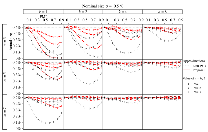
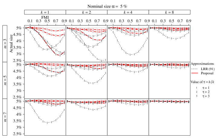
To compare the performance of $F_{k,\widehat{\operatorname{df}}(\mathcal{r}_{m},h)}$ in (2.15) with the existing best approximation $F_{k,\widetilde{\operatorname{df}}(\mathcal{r}_{m},h)}$, as approximations to the limiting distribution of $D$ given in (2.14), we compute via simulations

$$\widetilde{\alpha}=\operatorname{P}\left\{D>F^{-1}_{k,\widetilde{\operatorname{df}}(\mathcal{r}_{m},h)}(1-\alpha)\right\}\quad\text{and}\quad\widehat{\alpha}=\operatorname{P}\left\{D>F^{-1}_{k,\widehat{\operatorname{df}}(\mathcal{r}_{m},h)}(1-\alpha)\right\},$$

where $F^{-1}_{k,\operatorname{df}}(q)$ denotes the $q$-quantile of $F_{k,\operatorname{df}}$. Note that the experiments assess solely the performance of the finite-$m$ approximation instead of the performance of the large-$n$ $\chi^{2}$-approximation of the asymptotic LRT statistics. We draw $N=2^{18}$ independent copies $D$ for each of the following possible combinations: $m\in\{3,5,7\}$, $k\in\{1,2,4,8\}$, $\tau=h/k\in\{1,2,3\}$, $\mathcal{f}_{m}\in\{0,0.1,\ldots,0.9\}$, and following the recommendation of Benjamin et al. (2018), we use both $\alpha\in\{0.5\%,5\%\}$. The results for $\alpha=0.5\%$ and $\alpha=5\%$ are shown in Figure 1 and Figure 6 of the Appendix, respectively. In general, $\widehat{\alpha}$ approximates $\alpha$ much better than $\widetilde{\alpha}$ does, especially when $m,k,h$ are small. When $m,h$ are larger, they perform similarly because both $F_{k,\widetilde{\operatorname{df}}(\mathcal{r}_{m},h)}$ and $F_{k,\widehat{\operatorname{df}}(\mathcal{r}_{m},h)}$ get closer to $\chi^{2}_{k}/k$. However, the performance of $\widetilde{\alpha}$ and $\widehat{\alpha}$ is not monotonic in $\mathcal{f}_{m}$. The performance of $F_{k,\widehat{\operatorname{df}}(\mathcal{r}_{m},h)}$ is particularly good for $0\%\lesssim\mathcal{f}_{m}\lesssim 30\%$. Consequently, we recommend using $F_{k,\widehat{\operatorname{df}}(\widehat{r}_{\operatorname{L}}^{\operatorname{\lozenge}},h)}$ as an approximate null distribution for $\widehat{D}_{\operatorname{L}}^{\operatorname{\lozenge}}$, and $F_{k,\widehat{\operatorname{df}}(\widehat{r}_{\operatorname{L}}^{+},k)}$ for $\widehat{D}_{\operatorname{L}}^{+}$, as employed in the rest of this paper. However, these approximations obviously suffer from the usual “plug-in problem” by ignoring the uncertainty in estimating $\mathcal{r}_{m}$. Because $F_{k,{\rm df}}$ is not too sensitive to the value of ${\rm df}$ once it is reasonably large ($\operatorname{df}\geq 20$), the “plug-in problem” is less an issue here than in many other contexts, leading to acceptable approximations, as empirically demonstrated in Section 4. Nevertheless, further improvements should be sought, especially for dealing with the violation of the EFMI assumption, which would likely make the performance of our tests deteriorate with large $k$ or $h$, in contrast to the results shown in Figure 1; see Chan (2021) for a possible remedy.

3 Computational Considerations and Comparisons

3.1 Computationally Feasible Combining Rule

For many real-world data sets, $X$ is an $n\times p$ matrix, with rows indicating subjects and columns indicating attributes. We write $X=(X_{1},\ldots,X_{n})^{{\intercal}}$, and its sampling model by $f_{n}(X\mid\psi)$. Correspondingly, the $\ell$th imputed data set is $X^{(\ell)}=(X^{(\ell)}_{1},\ldots,X^{(\ell)}_{n})^{{\intercal}}$. Define the stacked data set by $X^{(1:m)}=[(X^{(1)})^{\intercal},\ldots,(X^{(m)})^{\intercal}]^{\intercal}$, a $mn\times p$ matrix, which is conceptually different from the collection of data sets $\{X^{(1)},\ldots,X^{(m)}\}$. Assuming that the rows of $X$ are independent, we can compute (2.1) as

$$\overline{L}(\psi)=\frac{1}{m}\log f_{mn}(X^{(1:m)}\mid\psi).$$ (3.1)

Consequently, as long as the user’s complete-data procedures can handle size $mn$ instead of $n$, the user can apply them to $X^{(1:m)}$ to obtain $\widehat{D}^{+}_{\operatorname{L}}$ and $\widehat{D}^{\operatorname{\lozenge}}_{\operatorname{L}}$ in (2.11).

In many applications, the rows correspond to individual subjects. Thus, the row-independence assumption typically holds for arbitrary $n$. Hence, we can extend from $n$ to $mn$, assuming the user’s complete-data procedure is not size-limited. Even if this is not true, (A.5) can still hold approximately under some regularity conditions; see Appendix A, where we also reveal a subtle, but important difference between the computation formulae (2.1) and (A.5).

Similar to $\mathcal{D}_{\operatorname{L}}$ in (1.12), we define complete-data functions

$$\mathcal{D}_{\operatorname{L},0}(X)=2\log f(X\mid\widehat{\psi}_{0}(X)),\quad\mathcal{D}_{\operatorname{L},1}(X)=2\log f(X\mid\widehat{\psi}(X)),$$ (3.2)

the only input of which is the data set $X$. Clearly, $\mathcal{D}_{\operatorname{L}}(X)=\mathcal{D}_{\operatorname{L},1}(X)-\mathcal{D}_{\operatorname{L},0}(X)$. The subroutine for evaluating the complete-data LRT function $X\mapsto\mathcal{D}_{\operatorname{L}}(X)$ is usually available, as is the subroutine for $X\mapsto\mathcal{D}_{\operatorname{L},1}(X)$, for example, the function logLik in R extracts the maximum of the complete data log-likelihood for objects belonging to classes "glm", "lm", "nls", and "Arima".

Algorithms 1 and 2 compute $\widehat{D}^{\operatorname{\lozenge}}_{\operatorname{L}}$ and $\widehat{D}_{\operatorname{L}}^{+}$, respectively. We recommend using the robust MI LRT in Algorithm 1, because it has the best theoretical guarantee. The second test can be useful when $\mathcal{D}_{\operatorname{L}}$ is available but $\mathcal{D}_{\operatorname{L},1}$ is not.

Input: Data sets $X^{(1)},\ldots,X^{(m)}$; $h,k$; functions $\mathcal{D}_{\operatorname{L},1}$, $\mathcal{D}_{\operatorname{L}}$ in (3.2), (1.12).

begin

       Stack the data sets to form $X^{(1:m)}=[(X^{(1)})^{\intercal},\ldots,(X^{(m)})^{\intercal}]^{\intercal}$.

       Find $\overline{\delta}_{\operatorname{L}}=\sum_{\ell=1}^{m}\mathcal{D}_{\operatorname{L},1}(X^{(\ell)})/m$, $\widehat{\delta}_{\operatorname{L}}=\mathcal{D}_{\operatorname{L},1}(X^{(1:m)})/m$, $\widehat{d}_{\operatorname{L}}=\mathcal{D}_{\operatorname{L}}(X^{(1:m)})/m$.

       Calculate $\widehat{r}_{\operatorname{L}}^{\operatorname{\lozenge}}$ according to (2.9), and $\widehat{D}^{\operatorname{\lozenge}}_{\operatorname{L}}$ according to (2.7) and (2.11).

       Calculate $\widehat{\operatorname{df}}(\widehat{r}^{\operatorname{\lozenge}}_{\operatorname{L}},h)$ according to (2.15).

       Compute the $p$-value as $1-F_{k,\widehat{\operatorname{df}}(\widehat{r}^{\operatorname{\lozenge}}_{\operatorname{L}},h)}(\widehat{D}_{\operatorname{L}}^{\operatorname{\lozenge}})$.

Algorithm 1 (Robust) MI LRT statistic $\widehat{D}^{\operatorname{\lozenge}}_{\operatorname{L}}$

Input: Data sets $X^{(1)},\ldots,X^{(m)}$; $k$; function $\mathcal{D}_{\operatorname{L}}$ in (1.12).

begin

       Stack the data sets to form $X^{(1:m)}=[(X^{(1)})^{\intercal},\ldots,(X^{(m)})^{\intercal}]^{\intercal}$.

       Find $\overline{d}_{\operatorname{L}}=\sum_{\ell=1}^{m}\mathcal{D}_{\operatorname{L}}(X^{(\ell)})/m$ and $\widehat{d}_{\operatorname{L}}=m^{-1}\mathcal{D}_{\operatorname{L}}(X^{(1:m)})$.

       Calculate $\widehat{r}_{\operatorname{L}}^{+}$ according to (2.8), and $\widehat{D}_{\operatorname{L}}^{+}$ according to (2.7) and (2.11).

       Calculate $\widehat{\operatorname{df}}(\widehat{r}^{+}_{\operatorname{L}},k)$ according to (2.15).

       Compute the $p$-value as $1-F_{k,\widehat{\operatorname{df}}(\widehat{r}^{+}_{\operatorname{L}},k)}(\widehat{D}_{\operatorname{L}}^{+}).$

Algorithm 2 MI LRT statistic $\widehat{D}_{\operatorname{L}}^{+}$

3.2 Computational Comparison with Existing Tests

Different MI tests require different computing subroutines, for example, $\mathcal{D}_{\operatorname{L}}$, $\widetilde{\mathcal{D}}_{\operatorname{L}}$, $\mathcal{D}_{\operatorname{L},1}$,

$$\mathcal{M}_{\operatorname{W}}(X)=\left\{\widehat{\theta}(X),U(X)\right\}\qquad\text{and}\qquad\mathcal{M}_{\operatorname{L}}(X)=\left\{\widehat{\psi}(X),\widehat{\psi}_{0}(X)\right\},$$

where the unnormalized density can be used in $\mathcal{D}_{\operatorname{L},1}$. We summarize the computing requirement in Table 1. We also compare the following statistical and computational properties of various MI test statistics and various estimators of $\mathcal{r}_{m}$:

• (Inv) The MI test is invariant to re-parametrization of $\psi$.

• (Con) The estimator of $\mathcal{r}_{m}$ is consistent, regardless of whether or not $H_{0}$ is true.

• ($\geq 0$) The test statistic and estimator of $\mathcal{r}_{m}$ are always non-negative.

• (Pow) The MI test has high power to reject $H_{0}$ under $H_{1}$.

• (Def) The MI test statistic is well defined and numerically well conditioned.

• (Sca) The MI procedure requires that users deal with scalars only.

• (EFMI) Whether EFMI is assumed for $\theta$ or for $\psi$.

Table 1: Computational requirements and statistical properties of MI tests. The symbol “$+$” (resp. “$-$”) means that a test has (resp. does not have) the indicated property; see Section 3.2 for detailed descriptions. WT-1 (Rubin, 2004; Li et al., 1991a) and LRT-1 (Meng and Rubin, 1992) are existing tests. LRT-2 and LRT-3 are the proposed tests, which can be computed by Algorithms 2 and 1, respectively. LRT-3 is recommended.

				Properties
Test	Statistic	Distribution	Routine	Inv	Con	$\geq 0$	Pow	Def	Sca	EFMI
WT-1	$D_{\operatorname{W}}(T)$	$\approx F_{k,\widetilde{\operatorname{df}}(\widetilde{r}_{\operatorname{W}}^{\prime},k)}$	$\mathcal{M}_{\operatorname{W}}$	$-$	$+$	$+$	$-$	$-$	$-$	$\theta$
LRT-1	$\widetilde{D}_{\operatorname{L}}(\widetilde{r}_{\operatorname{L}})$	$\approx F_{k,\widetilde{\operatorname{df}}(\widetilde{r}_{\operatorname{L}},k)}$	$\mathcal{M}_{\operatorname{L}},\widetilde{\mathcal{D}}_{\operatorname{L}}$	$-$	$-$	$-$	$-$	$+$	$-$	$\theta$
LRT-2	$\widehat{D}_{\operatorname{L}}(\widehat{r}^{+}_{\operatorname{L}})$	$\approx F_{k,\widehat{\operatorname{df}}(\widehat{r}_{\operatorname{L}}^{+},k)}$	$\mathcal{D}_{\operatorname{L}}$	$+$	$-$	$+$	$-$	$+$	$+$	$\theta$
LRT-3	$\widehat{D}_{\operatorname{L}}(\widehat{r}^{\operatorname{\lozenge}}_{\operatorname{L}})$	$\approx F_{k,\widehat{\operatorname{df}}(\widehat{r}_{\operatorname{L}}^{\operatorname{\lozenge}},k)}$	$\mathcal{D}_{\operatorname{L}},\mathcal{D}_{\operatorname{L},1}$	$+$	$+$	$+$	$+$	$+$	$+$	$\psi$

In summary, our proposed LRT-2 is the most attractive computationally. If the user is willing to make stronger assumptions, our proposed LRT-3 has better statistical properties, and is still computationally feasible. In practice, we recommend using LRT-3. We also present other existing MI tests and compare our proposals with them in Appendix A.5.

3.3 Summary of Notation

For ease of referencing, we summarize all major notation used in the paper. Recall that $\psi\in\mathbb{R}^{h}$ is the model parameter, and $\theta$ is the parameter of interest. We would like to test $H_{0}:\theta=\theta_{0}$ against $H_{1}:\theta\neq\theta_{0}$.

• Complete-data Estimators and Test Statistics:

  • $\widehat{\theta}(X)$ and $U(X)$: MLE of $\theta$ and its variance estimator.

  • $\widehat{\psi}(X)$ and $\widehat{\psi}_{0}(X)$: the unrestricted and $H_{0}$-restricted MLEs of $\psi$.

  • $d_{\operatorname{W}}(\widehat{\theta},U)=(\widehat{\theta}-\theta_{0})^{\intercal}U^{-1}(\widehat{\theta}-\theta_{0})$: the Wald test statistic.

  • $d_{\operatorname{L}}(\widehat{\psi}_{0},\widehat{\psi}\mid X)=2\log\{f(X\mid\widehat{\psi})/f(X\mid\widehat{\psi}_{0})\}$: the LRT statistic.

• Complete-data Functions (or Software Routines):

  • $\mathcal{M}_{\operatorname{W}}(X)=\{\widehat{\theta}(X),U(X)\}$ and $\mathcal{M}_{\operatorname{L}}(X)=\{\widehat{\psi}(X),\widehat{\psi}_{0}(X)\}$.

  • $\widetilde{\mathcal{D}}_{\operatorname{L}}(X,\psi_{0},\psi)=d_{\operatorname{L}}(\psi_{0},\psi\mid X)$: a nonstandard LRT function/routine.

  • $\mathcal{D}_{\operatorname{L}}(X)=d_{\operatorname{L}}(\widehat{\psi}_{0}(X),\widehat{\psi}(X)\mid X)$: the standard LRT function/routine.

  • $\mathcal{D}_{\operatorname{L},1}(X)=2\log f(X\mid\widehat{\psi}(X))$: the (scaled) maximum log-likelihood.

• MI Statistics:

  • $\widehat{\theta}^{(\ell)}$, $U^{(\ell)}$, $\widehat{\psi}_{0}^{(\ell)}$, $\widehat{\psi}^{(\ell)}$, $d^{(\ell)}_{\operatorname{W}}$, $d_{\operatorname{L}}^{(\ell)}$: the imputed values of $\widehat{\theta}$, $U$, $\widehat{\psi}_{0}$, $\widehat{\psi}$, $d_{\operatorname{W}}(\widehat{\theta},U)$, $d_{\operatorname{L}}(\widehat{\psi}_{0},\widehat{\psi}\mid X)$ using the imputed data set $X^{(\ell)}$ for each $\ell$.

  • $\overline{\theta}$, $\overline{U}$, $\overline{\psi}_{0}$, $\overline{\psi}$, $\overline{d}_{\operatorname{W}}$, $\overline{d}_{\operatorname{L}}$: the averages (over $\ell$) of $\widehat{\theta}^{(\ell)}$, $U^{(\ell)}$, $\widehat{\psi}_{0}^{(\ell)}$, $\widehat{\psi}^{(\ell)}$, $d^{(\ell)}_{\operatorname{W}}$, $d_{\operatorname{L}}^{(\ell)}$.

  • $T=\overline{U}+(1+1/m)B$, where $B=\sum_{\ell=1}^{m}(\widehat{\theta}^{(\ell)}-\overline{\theta})(\widehat{\theta}^{(\ell)}-\overline{\theta})^{\intercal}/(m-1)$.

  • $\overline{d}_{\operatorname{W}}^{\prime}=\sum_{\ell=1}^{m}d_{\operatorname{W}}(\widehat{\theta}^{(\ell)},\overline{U})/m$ and $\widetilde{d}_{\operatorname{W}}^{\prime}=d_{\operatorname{W}}(\overline{\theta},\overline{U})$.

  • $\widetilde{d}_{\operatorname{L}}=\sum_{\ell=1}^{m}\widetilde{\mathcal{D}}_{\operatorname{L}}(X^{(\ell)},\overline{\psi}_{0},\overline{\psi})/m$: an existing pooled LRT statistic.

  • $\widehat{d}_{\operatorname{L}}=\mathcal{D}_{\operatorname{L}}(X^{(1:m)})/m$: the proposed pooled LRT statistic.

  • $\overline{\delta}_{\operatorname{L}}=\sum_{\ell=1}^{m}\mathcal{D}_{\operatorname{L},1}(X^{(\ell)})/m$ and $\widehat{\delta}_{\operatorname{L}}=\mathcal{D}_{\operatorname{L},1}(X^{(1:m)})/m$: two proposed ways for pooling maximized log-likelihood.

• Estimators of $\mathcal{r}_{m}$:

  • $\widetilde{r}_{\operatorname{W}}^{\prime}=(m+1)(\overline{d}_{\operatorname{W}}^{\prime}-\widetilde{d}_{\operatorname{W}}^{\prime})/\{k(m-1)\}$ (Rubin, 2004).

  • $\widetilde{r}_{\operatorname{L}}=(m+1)(\overline{d}_{\operatorname{L}}-\widetilde{d}_{\operatorname{L}})/\{k(m-1)\}$ (Meng and Rubin, 1992).

  • $\widehat{r}_{\operatorname{L}}^{+}=\max[0,(m+1)(\overline{d}_{\operatorname{L}}-\widehat{d}_{\operatorname{L}})/\{k(m-1)\}]$: our first proposal.

  • $\widehat{r}_{\operatorname{L}}^{\operatorname{\lozenge}}=(m+1)(\overline{\delta}_{\operatorname{L}}-\widehat{\delta}_{\operatorname{L}})/\{h(m-1)\}$: our second proposal.

• MI Test Statistics for Testing $H_{0}$ against $H_{1}$:

  • (WT-1) $D_{\operatorname{W}}(T)=d_{\operatorname{W}}(\overline{\theta},T)/k$: the classical MI Wald test.

  • (LRT-1) $\widetilde{D}_{\operatorname{L}}(\widetilde{r}_{\operatorname{L}})={\widetilde{d}_{\operatorname{L}}}/\{k(1+\widetilde{r}_{\operatorname{L}})\}$: the existing MI LRT.

  • (LRT-2) $\widehat{D}_{\operatorname{L}}(\widehat{r}_{\operatorname{L}}^{+})={\widehat{d}_{\operatorname{L}}}/\{k(1+\widehat{r}_{\operatorname{L}}^{+})\}$: our first proposal.

  • (LRT-3) $\widehat{D}_{\operatorname{L}}(\widehat{r}_{\operatorname{L}}^{\operatorname{\lozenge}})={\widehat{d}_{\operatorname{L}}}/\{k(1+\widehat{r}_{\operatorname{L}}^{\operatorname{\lozenge}})\}$: our second proposal.

4 Empirical Investigation and Findings

4.1 Monte Carlo Experiments With EFMI

Let $X_{1},\ldots,X_{n}\sim\mathcal{N}_{p}(\mu,\Sigma)$ independently, where $\mu=(\mu_{1},\ldots,\mu_{p})^{{\intercal}}$. Assume that only $n_{\operatorname{obs}}=\lfloor(1-\mathcal{f})n\rfloor$ data points are observed. Let $X_{\operatorname{obs}}=\{X_{i}:i=1,\ldots,n_{\operatorname{obs}}\}$ and $X_{\operatorname{mis}}=\{X_{i}:i=n_{\operatorname{obs}}+1,\ldots,n\}$. We want to test $H_{0}:\mu_{1}=\cdots=\mu_{p}$.

Obviously, one may directly use the observed data set to construct the LRT statistic $D_{\operatorname{L}}$ without MI. Thus, it is regarded as a benchmark (denoted by LRT-0). The tests WT-1 and LRT-1,2,3 listed in Table 1 are investigated. We perform MI using a Bayesian model with a multivariate Jeffreys prior on $(\mu,\Sigma)$, this is, $f(\mu,\Sigma)\propto|\Sigma|^{-(p+1)/2}$. The imputation procedure is detailed in Appendix A.6. We study the impact of the parametrization on different test statistics.

• Parametrizations of $\theta$ for the Wald tests: (i) $\theta=\left(\mu_{2}-\mu_{1},\ldots,\mu_{p}-\mu_{p-1}\right)^{{\intercal}}$; (ii) $\theta=\left(\mu_{2}/\mu_{1}-1,\ldots,\mu_{p}/\mu_{p-1}-1\right)^{{\intercal}}$; and (iii) $\theta=\left(\mu_{2}^{3}-\mu_{1}^{3},\ldots,\mu_{p}^{3}-\mu_{p-1}^{3}\right)^{{\intercal}}$. For any case above, $H_{0}$ can be expressed as $\theta=(0,\ldots,0)^{{\intercal}}$.

• Parametrizations of $\psi$ for LRTs: (i) $\psi=\left\{\mu;\Sigma\right\}$; (ii) $\psi=\{\sqrt{\sigma_{ii}}/\mu_{i},1\leq i\leq p;\Sigma\}$; and (iii) $\psi=\left\{\mu^{{\intercal}}\Sigma^{-1/2};\Sigma^{-1}\right\}$, where $\Sigma=(\sigma_{ij})$ and $\Sigma^{1/2}$ is the square root of $\Sigma$ via the spectral method. The dimension of $\psi$ is $h=(p^{2}+3p)/2$.

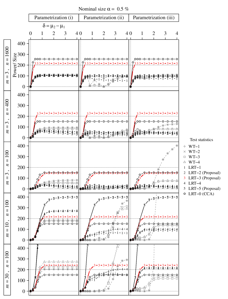
We set $\Sigma=\sigma^{2}\{(1-\rho)I_{p}+\rho\mathbf{1}_{p}\mathbf{1}_{p}^{{\intercal}}\}$, $\mathcal{f}=0.5$, $p=2$, $\rho=0.8$, $\sigma^{2}=5$, and $\mu=(-2+\delta,-2+2\delta)^{{\intercal}}$ for different values of $m\in\{3,10,30\}$, $n\in\{100,400,1600\}$, and $\delta=\mu_{2}-\mu_{1}\in[0,4]$. All simulations are repeated $2^{12}$ times. The empirical power functions for $\alpha=0.5\%$ tests are plotted in Figure 2. The results for $\alpha=5\%$ tests are deferred to Table 10 of the Appendix.

Figure 2: The power curves under nominal size $\alpha=0.5\%$. In each plot, the vertical axis denotes the power, and the horizontal axis denotes the value of $\delta=\mu_{2}-\mu_{1}$.

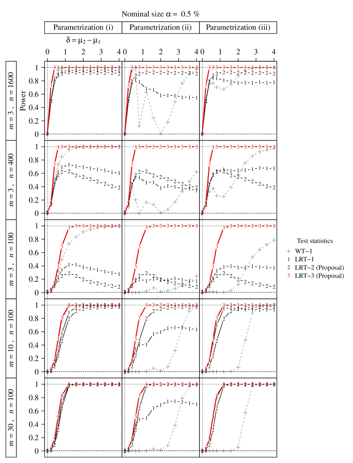
In general, WT-1 exhibits monotonically increasing power as $\delta$ increases, and its performance is affected significantly by parametrization. Indeed, the power can be as low as zero when $1\lesssim\delta\lesssim 2$ under parametrizations (ii) and (iii). Under parametrization (ii), LRT-1 is not powerful, even for large $\delta$. On the other hand, our first proposed test statistic LRT-2 performs better than LRT-1, at least for large $m$; however, they also lose a significant amount of power when $m$ is small. Our recommended proposal LRT-3 performs best in all cases. The superiority of LRT-3 is particularly striking when $m$ is small, this is, $m=3$.

We also investigate (a) the distribution of the $p$-value, (b) the empirical size $\widehat{\alpha}$ in comparison to the nominal type-I error $\alpha$, (c) the empirical size-adjusted power (Bayarri et al., 2016), (d) the robustness of our proposed estimators of $\mathcal{r}_{m}$, and (e) the performance of other existing MI tests. The results are shown in Appendix A.6, all of which indicate that our proposed tests perform best.

4.2 Monte Carlo Experiments Without EFMI

To check how robust various tests are to the assumption of EFMI, we simulate $X_{i}=(X_{i1},\ldots,X_{ip})^{{\intercal}}\sim\mathcal{N}_{p}(\mu,\Sigma)$ independently for $i=1,\ldots,n$. Let $R_{ij}$ be defined by $R_{ij}=1$ if $X_{ij}$ is observed, and $R_{ij}=0$ otherwise. Suppose that the first variable $X_{\cdot 1}$ is always observed, and the rest form a monotone missing pattern, as defined by a logistic model on the missing propensity: $\operatorname{P}\left(R_{ij}=0\mid R_{i,j-1}=a\right)=\left[1+\exp(\alpha_{0}+\alpha_{1}X_{i,j-1})\right]^{-1}$ (for $j=2,\ldots,p$) when $a=1$. This probability is zero when $a=0$ (i.e., nothing is missing). If $\alpha_{1}=0$, the data are missing completely at random (MCAR); otherwise they are missing at random (MAR); see Rubin (1976). The imputation procedure is given in Appendix A.7.

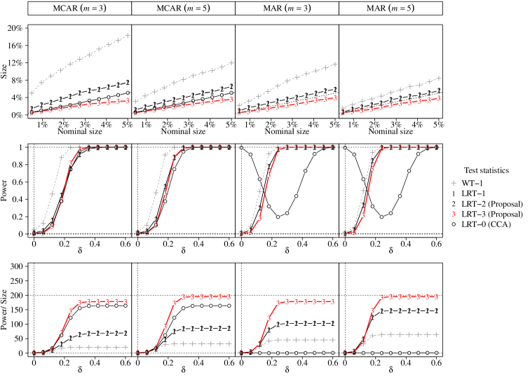
We test $H_{0}:\mu=\bm{0}_{p}$ against $H_{1}:\mu\not{=}\bm{0}_{p}$. We set $\mu=\delta\bm{1}_{p}$, where $\delta\in[0,0.6]$; $\Sigma_{ij}=0.5^{|i-j|}$, for $i,j=1,\ldots,p$; $n=500$; $m\in\{3,5\}$; $p=5$; and $(\alpha_{0},\alpha_{1})\in\{(2,-1),(1,0)\}$. Our model treats $\Sigma$ as unknown, and hence $k=p$ and $h=(3p+p^{2})/2$. Under $H_{0}$ and MAR, the FMI, i.e., the eigenvalues of $\mathcal{B}_{\theta}\mathcal{T}_{\theta}^{-1}$, are $(0,19\%,34\%,45\%,55\%)$. Thus, the assumption of EFMI does not hold.

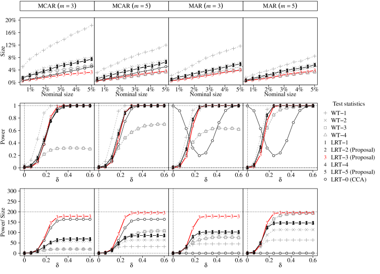
In this experiment, we also compare the performance of WT-1 and LRT-1,2,3. For reference, the complete-case (asymptotic) LRT using $\left\{X_{i}:R_{i1}=\cdots=R_{ip}=1\right\}$, denoted by LRT-0, is also computed. The results are shown in Figure 3. The size of LRT-3 is accurate when the nominal size is small. If the data are MCAR, LRT-0 is valid, but with slightly less power. (LRT-0 is typically invalid without MCAR.) The test LRT-3 has the best power-to-size ratio among all other tests. The power-to-size ratio of LRT-2 and LRT-3 become closer to the nominal value $1/0.5\%=200$ as $m$ increases. These results indicate that our proposed tests perform well and best, despite the serious violation of the EFMI assumption.

Figure 3: The empirical size, empirical power, and their ratio. The first row of plots show the empirical sizes. The size of the complete-case test (C2) under MAR is off the chart (always equal to one) because it is invalid. The second and third rows of plots show the powers and the power-to-size ratios, respectively. The nominal size is $0.5\%$.

5 Conclusion, Limitation and Future Work

In addition to conducting a general comparative study of MI tests, we have proposed two particularly promising MI LRTs based on $\widehat{D}_{\operatorname{L}}^{\operatorname{\lozenge}}=\widehat{D}_{\operatorname{L}}(\widehat{r}^{\operatorname{\lozenge}}_{\operatorname{L}})$ and $\widehat{D}_{\operatorname{L}}^{+}=\widehat{D}_{\operatorname{L}}(\widehat{r}^{+}_{\operatorname{L}})$. Both test statistics are non-negative, invariant to parametrizations, and powerful to reject a false $H_{0}$ (at least for large enough $m$). The test $\widehat{D}_{\operatorname{L}}^{\operatorname{\lozenge}}$ is the most principled, and has desirable monotonically increasing power as $H_{1}$ departs from $H_{0}$. However, it is derived under the stronger assumption of EFMI for $\psi$, not just for $\theta$. Furthermore, row independence of $X_{\operatorname{com}}$ is needed for ease of computation. (With a slightly more computationally demanding requirement, $\widehat{D}_{\operatorname{L}}(\widehat{r}^{\operatorname{\lozenge}}_{\operatorname{L}})$ can be used without the independence assumption.) The main advantage of $\widehat{D}_{\operatorname{L}}^{+}$ is that it is easier to compute, because it requires only standard complete-data computer subroutines for LRTs. One drawback is that the ad hoc fix $\widehat{r}^{+}_{\operatorname{L}}=\max(0,\widehat{r}_{\operatorname{L}})$ is inconsistent, in general. However, the inconsistency does not significantly affect the asymptotic power, at least in our experiments. Although $\widehat{D}_{\operatorname{L}}^{+}$ and $\widehat{D}_{\operatorname{L}}^{\operatorname{\lozenge}}$ offer significant improvements over existing options, more research is needed, for the reasons listed below:

• When the missing-data mechanism is not ignorable, but the imputers fail to fully take that into account, the issue of uncongeniality becomes critical (Meng, 1994a). Xie and Meng (2017) provide theoretical tools to address this issue in the context of estimation, and research is needed to extend their findings to the setting of hypothesis testing.

• Violating the EFMI assumption may not invalidate a test, but it will affect its power. Thus, it is desirable to explore MI tests without assuming EFMI.

• The robust $\widehat{D}_{\operatorname{L}}^{\operatorname{\lozenge}}$ relies on a stronger assumption of EFMI on $\psi$. We can modify it so only EFMI on $\theta$ is required, but the modification may be very difficult to compute, and may require that users have access to nontrivial complete-data procedures. Hence, a computationally feasible robust test that only assumes EFMI on $\theta$ needs to be developed.

• Because the FMI is a fundamental nuisance parameter and there is no (known) pivotal quantity, all MI tests are just approximations. If FMI is large or $m$ is small, they may perform poorly. Thus, seeking powerful MI tests that are least affected by FMI is of both theoretical and practical interest.

Supplementary Material
Appendix A contains additional theoretical results and details of numerical examples. Appendix B contains proofs of the main results. The R code is provided online.

Acknowledgments
Meng thanks the NSF and JTF for their partial financial support. He is also grateful for Keith’s (Kin Wai’s) creativity and diligence, which led to the remedies presented here, and which are also a part of Keith’s thesis. Chan thanks the University Grant Committee of HKSAR for its partial financial support.

Department of Statistics, The Chinese University of Hong Kong. E-mail: kinwaichan@cuhk.edu.hk Department of Statistics, Harvard University. E-mail: meng@stat.harvard.edu

Supplementary Material

Appendix A Supplementary Results

A.1 A Complication Caused by Nuisance Parameter

This section supplement the discussion of Section 2.2 in the main article. Recall that the likelihood function $L^{(\ell)}(\cdot)$ is based on both observed data $X_{\operatorname{obs}}$ and imputed data $X_{\operatorname{mis}}^{(\ell)}$, which varies across $\ell$. Hence, each imputed likelihood $L^{(\ell)}(\cdot)$ is associated with a (imputation-specific) pseudo parameter $\psi^{(\ell)}$, may vary across $\ell=1,\ldots,m$.

To see the source of the negativity of $\widehat{r}_{\operatorname{L}}$, we extend $\overline{L}(\psi)$ in (2.1) to

$$\overline{L}(\psi^{(1)},\ldots,\psi^{(m)})=\frac{1}{m}\sum_{\ell=1}^{m}L^{(\ell)}(\psi^{(\ell)}).$$ (A.1)

Using the “log-likelihood” $\overline{L}(\psi^{(1)},\ldots,\psi^{(m)})$, we can construct, at least conceptually, four hypotheses $H_{0}^{0}$, $H_{0}^{1}$, $H_{1}^{0}$, $H_{1}^{1}$ defined in Table 2. Each of them consists of zero, one or two of the constraints $\mathcal{C}_{0}:\theta^{(1)}=\cdots=\theta^{(m)}=\theta_{0}$ and $\mathcal{C}^{0}:\psi^{(1)}=\cdots=\psi^{(m)}$, where $\theta^{(\ell)}=\theta(\psi^{(\ell)})$ is the interested part of $\psi^{(\ell)}$ for each $\ell$. The constraint $\mathcal{C}_{0}$ is equivalent to $H_{0}$, and the constraint $\mathcal{C}^{0}$ means that all $\psi^{(\ell)}$s are equal, and hence it is effectively equivalent to $\mathcal{r}=0$, i.e., no missing information. The relationships among $H_{0}^{0}$, $H_{0}^{1}$, $H_{1}^{0}$, $H_{1}^{1}$ can be visualized in Figure 5. Define the maximized value of $\overline{L}(\psi^{(1)},\ldots,\psi^{(m)})$ under hypothesis $H\in\{H_{0}^{0},H_{0}^{1},H_{1}^{0},H_{1}^{1}\}$ by $\mathbb{L}(H)$. Then we can re-express $(\overline{d}_{\operatorname{L}}-\widehat{d}_{\operatorname{L}})/2$ as

$$(\overline{d}_{\operatorname{L}}-\widehat{d}_{\operatorname{L}})/2=\left\{\mathbb{L}(H_{1}^{1})-\mathbb{L}(H_{1}^{0})\right\}-\left\{\mathbb{L}(H_{0}^{1})-\mathbb{L}(H_{0}^{0})\right\}.$$ (A.2)

Whereas the two bracketed terms in (A.2) are non-negative as they correspond to two LRT statistics, their difference can be negative.

A simple example illustrates this well. For the regression model $[Y\mid X_{1},X_{2}]\sim\mathcal{N}(\beta_{0}+\beta_{1}X_{1}+\beta_{2}X_{2},\sigma^{2})$, the LRT statistic for testing $H_{1}^{0}:\beta_{1}=0,\beta_{2}\in\mathbb{R}$ against $H_{1}^{1}:\beta_{1},\beta_{2}\in\mathbb{R}$ is not necessarily larger (or smaller) than that for testing $H_{0}^{0}:\beta_{1}=\beta_{2}=0$ against $H_{0}^{1}:\beta_{1}\in\mathbb{R},\beta_{2}=0$; see Figure 4 for a schematic illustration.

Figure 4: A schematic illustration of the sign of (A.2). The contour lines of $\overline{L}(\psi^{(1)},\ldots,\psi^{(m)})$ are plotted. The two straight lines refer to constraints $\mathcal{C}_{0}$ and $\mathcal{C}^{0}$. Since $\mathbb{L}(H_{1}^{1})=0.082$, $\mathbb{L}(H_{0}^{1})=\mathbb{L}(H_{1}^{0})=0.08$, and $\mathbb{L}(H_{0}^{0})=0.01$, we have $\left\{\mathbb{L}(H_{1}^{1})-\mathbb{L}(H_{1}^{0})\right\}-\left\{\mathbb{L}(H_{0}^{1})-\mathbb{L}(H_{0}^{0})\right\}=0.002-0.007<0$. Note that the function $\overline{L}(\psi^{(1)},\ldots,\psi^{(m)})$ in (A.1) is at least $4$-dimensional (i.e., $\theta^{(1)},\theta^{(2)},\eta^{(1)},\eta^{(2)}$) generally, so this illustration in a $2$-dimension space is just conceptual.

Table 2: The definitions of hypotheses $H_{0}^{0}$, $H_{0}^{1}$, $H_{1}^{0}$, $H_{1}^{1}$.

	$\begin{array}[]{c}\mathcal{C}^{0}:\psi^{(1)}=\cdots=\psi^{(m)}\in\Psi\\ \text{(i.e., $\mathcal{r}=0$)}\end{array}$	$\begin{array}[]{c}\mathcal{C}^{1}:\psi^{(1)},\ldots,\psi^{(m)}\in\Psi\\ \text{(i.e., $\mathcal{r}\geq 0$)}\end{array}$
$\begin{array}[]{c}\mathcal{C}_{0}:\theta^{(1)}=\cdots=\theta^{(m)}=\theta_{0}\in\Theta\\ \text{(i.e., $H_{0}$-constrained)}\end{array}$	$H_{0}^{0}=\mathcal{C}_{0}\cap\mathcal{C}^{0}$	$H_{0}^{1}=\mathcal{C}_{0}\cap\mathcal{C}^{1}$
$\begin{array}[]{c}\mathcal{C}_{1}:\theta^{(1)},\ldots,\theta^{(m)}\in\Theta\\ \text{(i.e., not $H_{0}$-constrained)}\end{array}$	$H_{1}^{0}=\mathcal{C}_{1}\cap\mathcal{C}^{0}$	$H_{1}^{1}=\mathcal{C}_{1}\cap\mathcal{C}^{1}$

Figure 5: The relationships between the four hypotheses $H_{0}^{0}$, $H_{0}^{1}$, $H_{1}^{0}$, $H_{1}^{1}$. Each arrow denotes an implication, e.g., $H_{0}^{0}\Rightarrow H_{0}^{1}$ means that $H_{0}^{0}$ implies $H_{0}^{1}$.

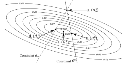
The decomposition (A.2) provides another interpretation of $\widehat{r}_{\operatorname{L}}$. The test statistic $\mathbb{L}(H_{1}^{1})-\mathbb{L}(H_{1}^{0})$ seeks evidence for detecting the falsity of $\mathcal{r}=0$ in both $\theta$ and $\eta$, whereas $\mathbb{L}(H_{0}^{1})-\mathbb{L}(H_{0}^{0})$ seeks evidence only in $\eta$. For cases where $\theta$ and $\eta$ are orthogonal (at least locally), the left-hand side of (A.2) can be viewed as a measure of evidence against $\mathcal{r}=0$ solely from $\theta$; Proposition 1 already hinted this possibility. However, the “test statistic” (A.2) has a fatal flaw. Because $\mathcal{C}_{0}$ requires all $\theta^{(\ell)}$s to coincide with a specific $\theta_{0}$, $\mathcal{C}_{0}$ is not nested within $\mathcal{C}^{0}$, i.e., $\mathcal{C}^{0}\nRightarrow\mathcal{C}_{0}$. Hence $\widehat{r}_{\operatorname{L}}$ is guaranteed to consistently estimate $\mathcal{r}_{m}$ only under $H_{0}$. This explains Corollary 1, and leads to an improvement in Section 2.2. In it not hard to see that our new estimator $\widehat{r}_{\operatorname{L}}^{\operatorname{\lozenge}}$ simply drops the second term in (A.2).

A.2 Another Motivation for $\widehat{r}_{\operatorname{L}}^{\operatorname{\lozenge}}$

The definition of $\widehat{r}_{\operatorname{L}}^{\operatorname{\lozenge}}$ can also be motivated by the following observation. First, observe that one simple method to construct an always non-negative estimator of $\mathcal{r}_{m}$ is to perturb $\widehat{\psi}_{0}^{*}$ and $\widehat{\psi}_{0}^{(\ell)}$ by a suitable amount, say $\Delta$, so that the perturbed version of $\widehat{r}_{\operatorname{L}}$ is always non-negative, and is still asymptotically equivalent to the original $\widehat{r}_{\operatorname{L}}$. We show, in Theorem 5 below, that the right amount of $\Delta$ is $\Delta=\widehat{\psi}^{*}-\widehat{\psi}_{0}^{*}$. Using the perturbed version of $\widehat{r}_{\operatorname{L}}$, we obtain

$$\widehat{r}_{\operatorname{L}}^{\operatorname{\triangle}}=\frac{m+1}{k(m-1)}\widehat{\delta}_{\operatorname{L}}^{\operatorname{\triangle}},$$

where

$$\widehat{\delta}_{\operatorname{L}}^{\operatorname{\triangle}}=\frac{2}{m}\sum_{\ell=1}^{m}\log\left\{\frac{f(X^{(\ell)}\mid\widehat{\psi}^{(\ell)})}{f(X^{(\ell)}\mid\widehat{\psi}^{*})}\frac{f(X^{(\ell)}\mid\widehat{\psi}_{0}^{*}+\Delta)}{f(X^{(\ell)}\mid\widehat{\psi}_{0}^{(\ell)}+\Delta)}\right\}=\frac{1}{m}\sum_{\ell=1}^{m}d_{\operatorname{L}}(\widehat{\psi}^{(\ell)}_{0}+\Delta,\widehat{\psi}^{(\ell)}\mid X^{(\ell)}).$$

Then we have the following result.

Theorem 5.

Suppose $\operatorname{RC}_{\theta}$. Under $H_{0}$, we have (i) $\widehat{r}_{\operatorname{L}}^{\operatorname{\triangle}}\geq 0$ for all $m,n$; and (ii) $\widehat{r}_{\operatorname{L}}^{\operatorname{\triangle}}\bumpeq\widehat{r}_{\operatorname{L}}$ as $n\rightarrow\infty$ for each $m$.

Although $\widehat{r}_{\operatorname{L}}^{\operatorname{\triangle}}\geq 0$, it is only invariant to affine transformations, and not robust against $\theta_{0}$, and less computational feasible than $\widehat{r}_{\operatorname{L}}$; see Section 3. However, it gives us some insights on how to construct a potentially better estimator. Note that, in (A.2), the constrained MLE is not used in $d_{\operatorname{L}}(\cdot,\cdot\mid X^{(\ell)})$, but it is still always non-negative. We call this a “pseudo” LRT statistics. Then, $\widehat{\delta}_{\operatorname{L}}^{\operatorname{\triangle}}$ is just a multiple of an average of many “pseudo” LRT statistics. In order to find a good estimator of $\mathcal{r}_{m}$, we may seek for an estimator which admits this form. Indeed, our estimator $\widehat{r}^{\operatorname{\lozenge}}_{\operatorname{L}}$ also takes the same form:

$$\widehat{r}_{\operatorname{L}}^{\operatorname{\lozenge}}=\frac{m+1}{h(m-1)}\frac{1}{m}\sum_{\ell=1}^{m}d_{\operatorname{L}}(\widehat{\psi}^{*},\widehat{\psi}^{(\ell)}\mid X^{(\ell)}).$$

A.3 Additional result for Section 2.3

This section presents the additional simulation result for Section 2.3. The performance of different approximations to the reference null distribution when $\alpha=5\%$ is shown in Figure 6.

Figure 6: The performance of two approximate null distributions when the nominal size is $\alpha=5\%$. The vertical axis denotes $\widehat{\alpha}$ or $\widetilde{\alpha}$, and the horizontal axis denotes the value of $\mathcal{f}_{m}$. The number attached to each line denotes the value of $\tau=h/k$. The proposed approximation $\widehat{\alpha}$ is denoted by thick solid lines with triangles, and the existing approximation $\widetilde{\alpha}$ is denoted by thin dashed lines with circles.

A.4 Results for Dependent Data

This is a supplement for Section 3.1. If the data are not independent, then (A.5) is no longer true. In other words, $\overline{L}(\psi)\not\equiv\overline{L}^{\operatorname{S}}(\psi)$, where $\overline{L}(\psi)=\sum_{\ell=1}^{m}L^{(\ell)}(\psi)/m$ is defined in (2.1), and

$$\overline{L}^{\operatorname{S}}(\psi)=\frac{1}{m}\log f_{mn}(X^{(1:m)}\mid\psi).$$ (A.3)

In principle, $\overline{L}(\psi)$ should be used instead of the “stacked version” $\overline{L}^{\operatorname{S}}(\psi)$, however, the stacked one is much easier to compute. Because of this reason, it is of interest to see whether the stacked version can be used generally.

To begin with, we define the stacked version of all MI statistics when $\overline{L}^{\operatorname{S}}(\psi)$ is used instead of $\overline{L}(\psi)$. Let

$$\widehat{\psi}_{0}^{\operatorname{S}} =\operatorname*{arg\,max}_{\psi\in\Psi\;:\;\theta(\psi)=\theta_{0}}\overline{L}^{\operatorname{S}}(\psi), \widehat{\psi}^{\operatorname{S}} =\operatorname*{arg\,max}_{\psi\in\Psi}\overline{L}^{\operatorname{S}}(\psi);$$ (A.4)

$$\widehat{\delta}_{0,\operatorname{S}} =2\overline{L}^{\operatorname{S}}(\widehat{\psi}_{0}^{\operatorname{S}}), \widehat{\delta}_{\operatorname{S}} =2\overline{L}^{\operatorname{S}}(\widehat{\psi}^{\operatorname{S}}).$$ (A.5)

and

$$\widehat{D}_{\operatorname{S}}(\mathcal{r}_{m}) =\frac{\widehat{d}_{\operatorname{S}}}{k(1+\mathcal{r}_{m})}, \text{with $\widehat{d}_{\operatorname{S}}=\widehat{\delta}_{\operatorname{S}}-\widehat{\delta}_{0,\operatorname{S}}$ of (\ref{eqt:def_deltaHat01S})};$$ (A.6)

$$\widehat{r}_{\operatorname{S}} =\frac{m+1}{k(m-1)}(\overline{d}_{\operatorname{S}}-\widehat{d}_{\operatorname{S}}), \text{with $\overline{d}_{\operatorname{S}}=\overline{d}_{\operatorname{L}}$ of (\ref{eqt:def_psiHat_bardd})};$$ (A.7)

$$\widehat{r}_{\operatorname{S}}^{\operatorname{\lozenge}} =\frac{m+1}{h(m-1)}(\overline{\delta}_{\operatorname{S}}-\widehat{\delta}_{\operatorname{S}}), \text{with $\overline{\delta}_{\operatorname{S}}=\overline{\delta}_{\operatorname{L}}$ of (\ref{eqt:def_deltabarhatL})};$$ (A.8)

and $\widehat{r}^{+}_{\operatorname{S}}=\max(0,\widehat{r}_{\operatorname{S}})$. The stacked counterparts of $\widehat{D}^{\operatorname{\lozenge}}_{\operatorname{L}}$ and its existing counterparts $\widehat{D}_{\operatorname{L}}$ and $\widehat{D}^{+}_{\operatorname{L}}$ (see (2.11)) then are given by

$$\widehat{D}_{\operatorname{S}}^{\operatorname{\lozenge}}=\widehat{D}_{\operatorname{S}}(\widehat{r}^{\operatorname{\lozenge}}_{\operatorname{S}}),\qquad\widehat{D}_{\operatorname{S}}=\widehat{D}_{\operatorname{S}}(\widehat{r}_{\operatorname{S}}),\qquad\widehat{D}_{\operatorname{S}}^{+}=\widehat{D}_{\operatorname{S}}(\widehat{r}^{+}_{\operatorname{S}}).$$ (A.9)

The approximation $\widehat{d}_{\operatorname{L}}\bumpeq\widehat{d}_{\operatorname{S}}$ is still true under the following conditions.

Assumption 5.

1. Define $R(\psi)=\underline{\overline{L}}^{\operatorname{S}}(\psi)-\underline{\overline{L}}(\psi)$, where

   $$\underline{\overline{L}}(\psi)=(mn)^{-1}\sum_{\ell=1}^{m}\log f(X^{(\ell)}\mid\psi)\quad{\rm and}\quad\underline{\overline{L}}^{\operatorname{S}}(\psi)=(mn)^{-1}\log f(X^{\operatorname{S}}\mid\psi).$$

   For each $m$, as $n\rightarrow\infty$,

   $$\sup_{\psi\in\Psi}\left|R(\psi)\right|=O_{p}(1/n),\qquad\sup_{\psi\in\Psi}\left|\frac{\partial}{\partial\psi}R(\psi)\right|=O_{p}(1/n).$$

2. For each $m$, there exists a continuous function $\psi\mapsto\overline{\underline{\mathcal{L}}}(\psi)$, which is free of $n$ but may depend on $m$, such that, as $n\rightarrow\infty$,

   $$\sup_{\psi\in\Psi}\left|\underline{\overline{L}}(\psi)-\overline{\underline{\mathcal{L}}}(\psi)\right|=o_{p}(1).$$

3. Let $\psi_{0}^{*}=\operatorname*{arg\,max}_{\psi\in\Psi\;:\;\psi(\theta)=\theta_{0}}\overline{\underline{\mathcal{L}}}(\psi)$ and $\psi^{*}=\operatorname*{arg\,max}_{\psi\in\Psi}\overline{\underline{\mathcal{L}}}(\psi)$. For any fixed $m$, and for all $\varepsilon>0$, there exists $\delta>0$ such that

   $$\sup_{\begin{subarray}{c}\psi\in\Psi\,:\,|\psi_{0}^{*}-\psi|>\varepsilon\\ \theta(\psi)=\theta_{0}\end{subarray}}\left\{\overline{\underline{\mathcal{L}}}(\psi_{0}^{*})-\overline{\underline{\mathcal{L}}}(\psi)\right\}\geq\delta,\quad\sup_{\psi\in\Psi\,:\,|\psi^{*}-\psi|>\varepsilon}\left\{\overline{\underline{\mathcal{L}}}(\psi^{*})-\overline{\underline{\mathcal{L}}}(\psi)\right\}\geq\delta.$$

Conditions (b) and (c) in Assumption 5 are standard RCs that are usually assumed for M-estimators (see Section 5 of van der Vaart (2000)); whereas condition (a) is satisfied by many models (see Example A.1 below).

Theorem 6.

Suppose $\operatorname{RC}_{\theta}$ and Assumption 5. Under both $H_{0}$ and $H_{1}$, we have (i) $\widehat{d}_{\operatorname{S}},\widehat{r}_{\operatorname{S}}\geq 0$ for all $m,n$; (ii) $\widehat{d}_{\operatorname{S}},\widehat{r}_{\operatorname{S}}$ are invariant to the parametrization of $\psi$ for all $m,n$; and (iii) $\widehat{d}_{\operatorname{L}}\bumpeq\widehat{d}_{\operatorname{S}}$ and $\widehat{r}_{\operatorname{L}}\bumpeq\widehat{r}_{\operatorname{S}}$ as $n\rightarrow\infty$ for each $m$.

Theorem 6 implies that the handy test statistics $\widehat{D}_{\operatorname{S}}$ and $\widehat{D}_{\operatorname{S}}^{+}$ approximate $\widehat{D}_{\operatorname{L}}$ and $\widehat{D}_{\operatorname{L}}^{+}$ for dependent data, provided that Assumption 5 holds.

Example A.1.

Consider a stationary autoregressive model of order one. Suppose the complete data $X=(X_{1},\ldots,X_{n})^{{\intercal}}$ is generated as following: $X_{1}\sim\mathcal{N}(0,v^{2})$ and $[X_{i}|X_{i-1}]\sim\mathcal{N}(\phi X_{i-1},\sigma^{2})$ for $i\geq 2$, where $v^{2}={\sigma^{2}(1+\phi)}/{(1-\phi)}$. Then $\psi=(\phi,\sigma^{2})^{{\intercal}}$, and

$$\underline{\overline{L}}(\psi) = -\frac{1}{2}\log(2\pi)-\frac{1}{2n}\log v^{2}-\frac{1}{mn}\sum_{\ell=1}^{m}\frac{X_{1}^{(\ell)}}{2v^{2}}-\frac{n-1}{2n}\log\sigma^{2}$$

$$-\frac{1}{mn}\sum_{\ell=1}^{m}\sum_{i=2}^{n}\frac{(X_{i}^{(\ell)}-\phi X_{i-1}^{(\ell)})^{2}}{2\sigma^{2}},$$

$$\underline{\overline{L}}^{\operatorname{S}}(\psi) = -\frac{1}{2}\log(2\pi)-\frac{1}{2mn}\log v^{2}-\frac{(X_{1}^{(1)})^{2}}{2mnv^{2}}-\frac{mn-1}{2mn}\log\sigma^{2}$$

$$-\frac{1}{mn}\sum_{\ell=1}^{m}\sum_{i=2}^{n}\frac{(X_{i}^{(\ell)}-\phi X_{i-1}^{(\ell)})^{2}}{2\sigma^{2}}-\frac{1}{mn}\sum_{\ell=2}^{m}\frac{(X_{1}^{(\ell)}-\phi X_{n}^{(\ell-1)})^{2}}{2\sigma^{2}}.$$

Then, it is easy to see that condition (a) of Assumption 5 is satisfied.

A.5 Other existing MI tests

First, we list some existing estimators of $\mathcal{r}_{m}$. Let $s_{\operatorname{W},a}^{2}$ be the sample variances of $\{(d^{(\ell)}_{\operatorname{W}})^{a}\}_{\ell=1}^{m}$ for $a>0$. Rubin (2004) and Li et al. (1991a) proposed

$$\widetilde{r}_{\operatorname{W},1} = \frac{(1+1/m)s_{\operatorname{W},1}^{2}}{2\overline{d}_{\operatorname{W}}+\sqrt{\max\left\{0,4\overline{d}^{2}_{\operatorname{W}}-2ks_{\operatorname{W},1}^{2}\right\}}},$$ (A.10)

$$\widetilde{r}_{\operatorname{W},1/2} = (1+1/m)s_{\operatorname{W},1/2}^{2},$$ (A.11)

respectively. When $k$ is large and $m$ is small, using (A.10) or (A.11) may lead to power loss. A trivial modification of $\widetilde{r}_{\operatorname{L}}$ of (1.10), i.e., $\widetilde{r}^{+}_{\operatorname{L}}=\max(0,\widetilde{r}_{\operatorname{L}})$, is a better alternative.

Second, we list some alternative MI combining rules. Having the above estimators of $\mathcal{r}_{m}$, we can insert them into the following combining rules:

$$\widetilde{D}_{\operatorname{W}}^{\prime}(\mathcal{r}_{m})=\frac{\widetilde{d}_{\operatorname{W}}^{\prime}}{k(1+\mathcal{r}_{m})},\;\widetilde{D}_{\operatorname{L}}(\mathcal{r}_{m})=\frac{\widetilde{d}_{\operatorname{L}}}{k(1+\mathcal{r}_{m})},\;\widetilde{D}^{+}_{\operatorname{L}}(\mathcal{r}_{m})=\left\{\widetilde{D}_{\operatorname{L}}(\mathcal{r}_{m})\right\}^{+}.$$ (A.12)

Using (1.3) and (1.10), we can also define the following combining rules:

$$\overline{D}_{\operatorname{W}}^{\prime}(\mathcal{r}_{m})=\frac{\overline{d}_{\operatorname{W}}^{\prime}-\frac{k(m-1)}{m+1}\mathcal{r}_{m}}{k(1+\mathcal{r}_{m})},\qquad\overline{D}_{\operatorname{L}}(\mathcal{r}_{m})=\frac{\overline{d}_{\operatorname{L}}-\frac{k(m-1)}{m+1}\mathcal{r}_{m}}{k(1+\mathcal{r}_{m})};$$ (A.13)

see, e.g., Li et al. (1991a). The combining rule $\overline{D}_{\operatorname{W}}^{\prime}(\mathcal{r}_{m})$ is useful when computing $\overline{d}_{\operatorname{W}}^{\prime}$ and estimating $\mathcal{r}_{m}$ are simple, but the resulting power may deteriorate. If $\widetilde{r}_{\operatorname{W},1}$ or $\widetilde{r}_{\operatorname{W},1/2}$ is used for estimating $\mathcal{r}_{m}$, the null distribution of (A.12) and (A.13) can be approximated by $F_{k,\widetilde{\operatorname{df}}^{\prime}(\mathcal{r}_{m},k)}$, where $\widetilde{\operatorname{df}}^{\prime}(\mathcal{r}_{m},k)=(m-1)(1+\mathcal{r}_{m}^{-1})^{2}k^{-3/m}$; see Li et al. (1991a).

Next, we introduce and recall some notation: (a) standard complete-data moments estimation ($\mathcal{M}_{\operatorname{W}}$, $\mathcal{M}_{\operatorname{L}}$) and testing procedures ($\mathcal{D}_{\operatorname{W}}$, $\mathcal{D}_{\operatorname{L}}$), and (b) non-standard complete-data procedures ($\widetilde{\mathcal{D}}_{\operatorname{L}}$, $\overline{\mathcal{D}}_{\operatorname{L}}$, $\mathcal{D}_{\operatorname{L},1}$, $\overline{\mathcal{D}}_{\operatorname{L},1}$), where

$$\mathcal{M}_{\operatorname{W}}(X)=\left\{\widehat{\theta}(X),U(X)\right\},\quad\mathcal{M}_{\operatorname{L}}(X)=\left\{\widehat{\psi}(X),\widehat{\psi}_{0}(X)\right\},$$

$$\mathcal{D}_{\operatorname{W}}(X)=d_{\operatorname{W}}(\widehat{\theta}(X),U(X)),\quad\overline{\mathcal{D}}_{\operatorname{L},1}(\mathbb{X})=\frac{2}{m}\sum_{\ell=1}^{m}\log f(X^{(\ell)}\mid\widehat{\psi}^{*}(\mathbb{X})),$$

$$\overline{L}(\psi)=\frac{1}{m}\log f_{mn}(X^{(1:m)}\mid\psi).$$

Table 3 is the full version of Table 1 in the main text. It summarizes the statistical and computational properties of different MI tests; see Section 3.2 for details.

Table 3: Computational requirements and statistical properties of MI test statistics, their associated combining rules and estimators of FMI $\mathcal{r}_{m}$. The symbols “$+$” and “$-$” mean that the test statistic (or estimator) is equipped and not equipped with the indicated property, respectively; see the end of Section 3.2 for heading descriptions. The reference papers/book are abbreviated as follows: Rubin (2004) (R04), Li et al. (1991a) (LMRR91) and Meng and Rubin (1992) (MR92).

		Combining Rule		Estimator of $\mathcal{r}_{m}$		Approx. null distribution			Properties
Test	No.	Formula	Routine	Formula	Routine	Original	Proposed	Reference	Inv	Con	$\geq 0$	Pow	Def	Sca		EFMI
WT	WT-1	$D_{\operatorname{W}}(T)$	$\mathcal{M}_{\operatorname{W}}$	$\widetilde{r}^{\prime}_{\operatorname{W}}$	$\mathcal{D}_{\operatorname{W}}$	$F_{k,\widetilde{\operatorname{df}}(\mathcal{r}_{m},k)}$	$F_{k,\widehat{\operatorname{df}}(\mathcal{r}_{m},k)}$	R04	$-$	$+$	$+$	$-$	$-$	$-$		$\theta$
	WT-2	$\widetilde{D}^{\prime}_{\operatorname{W}}(\mathcal{r}_{m})$	$\mathcal{M}_{\operatorname{W}}$	$\widetilde{r}^{\prime}_{\operatorname{W}}$	$\mathcal{M}_{\operatorname{W}}$	$F_{k,\widetilde{\operatorname{df}}(\mathcal{r}_{m},k)}$	$F_{k,\widehat{\operatorname{df}}(\mathcal{r}_{m},k)}$	R04	$-$	$+$	$+$	$-$	$-$	$-$		$\theta$
	WT-3	$\widetilde{D}^{\prime}_{\operatorname{W}}(\mathcal{r}_{m})$	$\mathcal{M}_{\operatorname{W}}$	$\widetilde{r}^{\prime}_{\operatorname{W},1}$	$\mathcal{D}_{\operatorname{W}}$	$F_{k,\widetilde{\operatorname{df}}^{\prime}(\mathcal{r}_{m},k)}$	NA	R04	$-$	$-$	$+$	$-$	$-$	$-$		$\theta$
	WT-4	$\widetilde{D}^{\prime}_{\operatorname{W}}(\mathcal{r}_{m})$	$\mathcal{M}_{\operatorname{W}}$	$\widetilde{r}^{\prime}_{\operatorname{W},1/2}$	$\mathcal{D}_{\operatorname{W}}$	$F_{k,\widetilde{\operatorname{df}}^{\prime}(\mathcal{r}_{m},k)}$	NA	LMRR91	$-$	$-$	$+$	$-$	$-$	$-$		$\theta$
	WT-5	$\overline{D}^{\prime}_{\operatorname{W}}(\mathcal{r}_{m})$	$\mathcal{D}_{\operatorname{W}}$	$\widetilde{r}^{\prime}_{\operatorname{W},1}$	$\mathcal{D}_{\operatorname{W}}$	$F_{k,\widetilde{\operatorname{df}}^{\prime}(\mathcal{r}_{m},k)}$	NA	R04	$-$	$-$	$-$	$-$	$-$	$+$		$\theta$
	WT-6	$\overline{D}^{\prime}_{\operatorname{W}}(\mathcal{r}_{m})$	$\mathcal{D}_{\operatorname{W}}$	$\widetilde{r}^{\prime}_{\operatorname{W},1/2}$	$\mathcal{D}_{\operatorname{W}}$	$F_{k,\widetilde{\operatorname{df}}^{\prime}(\mathcal{r}_{m},k)}$	NA	LMRR91	$-$	$-$	$-$	$-$	$-$	$+$		$\theta$
LRT	LRT-1	$\widetilde{D}_{\operatorname{L}}(\mathcal{r}_{m})$	$\mathcal{M}_{\operatorname{L}},\widetilde{\mathcal{D}}_{\operatorname{L}}$	$\widetilde{r}_{\operatorname{L}}$	$\mathcal{M}_{\operatorname{L}},\widetilde{\mathcal{D}}_{\operatorname{L}}$	$F_{k,\widetilde{\operatorname{df}}(\mathcal{r}_{m},k)}$	$F_{k,\widehat{\operatorname{df}}(\mathcal{r}_{m},k)}$	MR92	$-$	$-$	$-$	$-$	$+$	$-$		$\theta$
	LRT-2	$\widehat{D}_{\operatorname{L}}(\mathcal{r}_{m})$	$\mathcal{D}_{\operatorname{L}}$	$\widehat{r}^{+}_{\operatorname{L}}$	$\mathcal{D}_{\operatorname{L}}$	$F_{k,\widetilde{\operatorname{df}}(\mathcal{r}_{m},k)}$	$F_{k,\widehat{\operatorname{df}}(\mathcal{r}_{m},k)}$	Proposal	$+$	$-$	$+$	$-$	$+$	$+$		$\theta$
	LRT-3	$\widehat{D}_{\operatorname{L}}(\mathcal{r}_{m})$	$\mathcal{D}_{\operatorname{L}}$	$\widehat{r}^{\operatorname{\lozenge}}_{\operatorname{L}}$	$\mathcal{D}_{\operatorname{L},1}$	$F_{k,\widetilde{\operatorname{df}}(\mathcal{r}_{m},h)}$	$F_{k,\widehat{\operatorname{df}}(\mathcal{r}_{m},h)}$	Proposal	$+$	$+$	$+$	$+$	$+$	$+$		$\psi$
	LRT-4	$\widetilde{D}^{+}_{\operatorname{L}}(\mathcal{r}_{m})$	$\mathcal{M}_{\operatorname{L}},\widetilde{\mathcal{D}}_{\operatorname{L}}$	$\widetilde{r}^{+}_{\operatorname{L}}$	$\mathcal{M}_{\operatorname{L}},\widetilde{\mathcal{D}}_{\operatorname{L}}$	$F_{k,\widetilde{\operatorname{df}}(\mathcal{r}_{m},k)}$	$F_{k,\widehat{\operatorname{df}}(\mathcal{r}_{m},k)}$	MR92	$-$	$-$	$+$	$-$	$+$	$-$		$\theta$
	LRT-5	$\widehat{D}_{\operatorname{L}}(\mathcal{r}_{m})$	$\mathcal{D}_{\operatorname{L}}$	$\widehat{r}_{\operatorname{L}}$	$\mathcal{D}_{\operatorname{L}}$	$F_{k,\widetilde{\operatorname{df}}(\mathcal{r}_{m},k)}$	$F_{k,\widehat{\operatorname{df}}(\mathcal{r}_{m},k)}$	Proposal	$+$	$-$	$-$	$-$	$+$	$+$		$\theta$

A.6 Supplement for Section 4.1

Let $\overline{X}_{\operatorname{obs}}$ and $S_{\operatorname{obs}}$ be the sample mean and sample covariance matrix based on ${X}_{\operatorname{obs}}$. Then, the $\ell$th imputed missing data set can be produced by the following procedure, for $\ell=1,\ldots,m$.

1. Draw $(\Sigma^{(\ell)})^{-1}$ from a Wishart distribution with $(n_{\operatorname{obs}}-1)$ degrees of freedom and scale matrix $S_{\operatorname{obs}}$.

2. Draw $\mu^{(\ell)}$ from $\mathcal{N}_{p}(\overline{X}_{\operatorname{obs}},\Sigma^{(\ell)}/n_{\operatorname{obs}})$.

3. Draw $(n-n_{\operatorname{obs}})$ imputed missing values $\{X^{(\ell)}_{i}:i=n_{\operatorname{obs}}+1,\ldots,n\}$ from $\mathcal{N}_{p}(\mu^{(\ell)},\Sigma^{(\ell)})$ independently.

Also, denote $X^{(\ell)}_{i}=X_{i}$ for $i=1,\ldots,n_{\operatorname{obs}}$. With the $\ell$th completed data set, the unconstrained MLEs for $\mu$ and $\Sigma$ are

$$\widehat{\mu}^{(\ell)}=\frac{1}{n}\sum_{i=1}^{n}X_{i}^{(\ell)},\qquad\widehat{\Sigma}^{(\ell)}=\frac{1}{n}\sum_{i=1}^{n}\left(X_{i}^{(\ell)}-\widehat{\mu}^{(\ell)}\right)\left(X_{i}^{(\ell)}-\widehat{\mu}^{(\ell)}\right)^{{\intercal}}.$$

Whereas we generate data using a covariance matrix with common variance and correlation, our model does not assume any structure for $\Sigma$. The only restriction we can impose is the common-mean assumption under the null, for which the constrained MLEs are

$$\widehat{\mu}^{(\ell)}_{0}=\left\{\frac{\mathbf{1}_{p}^{{\intercal}}(\widehat{\Sigma}^{(\ell)})^{-1}\widehat{\mu}^{(\ell)}}{\mathbf{1}_{p}^{{\intercal}}(\widehat{\Sigma}^{(\ell)})^{-1}\mathbf{1}_{p}}\right\}\mathbf{1}_{p},\qquad\widehat{\Sigma}^{(\ell)}_{0}=\widehat{\Sigma}^{(\ell)}+\left(\widehat{\mu}^{(\ell)}-\widehat{\mu}^{(\ell)}_{0}\right)\left(\widehat{\mu}^{(\ell)}-\widehat{\mu}^{(\ell)}_{0}\right)^{{\intercal}}.$$

Table 4: The values of parameters used in the simulation experiment in Section 4.1.

Experiment		Fixed Parameters			Variable Parameter
No.	Variable Parameter	$\rho$	$p$	$\mathcal{f}$	Case 1	Case 2	Case 3	Case 4	Case 5
I	Correlation $\rho$	–	$2$	$0.5$	$-0.8$	$-0.4$	$0$	$0.4$	$0.8$
II	Dimension $p$	$0.4$	–	$0.5$	$2$	$3$	$4$	$5$	$6$
III	FMI $\mathcal{f}$	$0.4$	$2$	–	$0.1$	$0.3$	$0.5$	$0.7$	$0.9$

We first study the distribution of $p$-values of each test under $H_{0}$. We use $n=100$, $m=3$, $\sigma^{2}=5$ and $\mu=\mathbf{1}_{p}$, with various values of $\rho$, $p$ and $\mathcal{f}$ specified in Table 4. The results under parametrizations (i), (ii) and (iii) are shown in Figures 7, 8 and 9, respectively. Note that, for Wald tests under parametrization (ii), the matrix $U^{(\ell)}$ is singular in $0.25\%$ of the replications, and those cases are removed from the analysis (which should favor the Wald tests).

Figure 7: The comparison between empirical size and nominal size $\alpha$ under parametrization (ii) for $\alpha\in(0,5\%]$. Our most recommended proposal is LRT-3, which is highlighted red.

Figure 8: The comparison between empirical size and nominal size $\alpha$ under parametrization (i) for $\alpha\in(0,5\%]$. The legend in Figure 7 also applies here.

Figure 9: The comparison between empirical size and nominal size $\alpha$ under parametrization (iii) for $\alpha\in(0,5\%]$. The legend in Figure 8 also applies here.

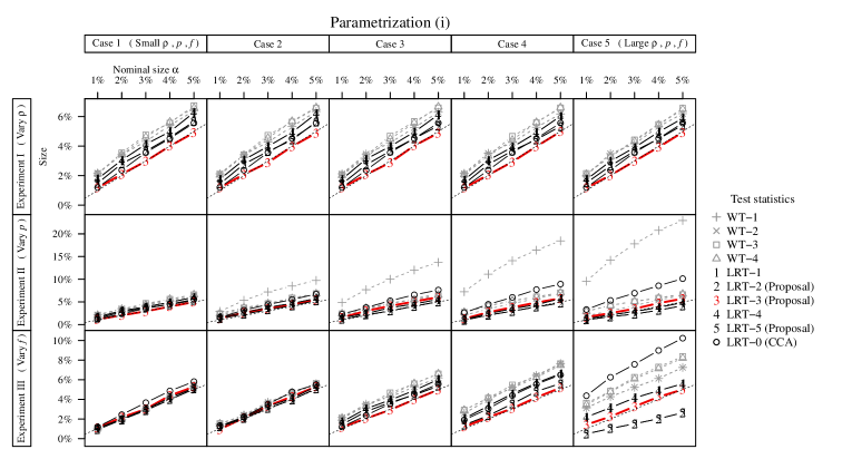
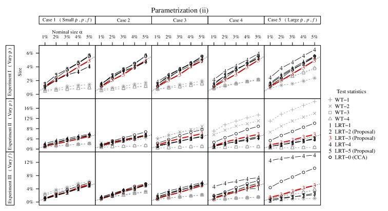
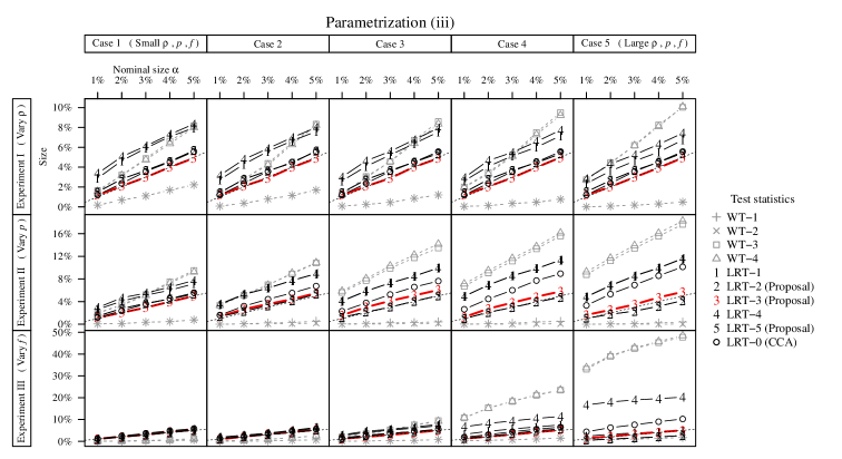
The empirical sizes (i.e., type-I errors) of the MI Wald tests generally deviate from the nominal size $\alpha$ under parametrization (ii). In contrast, the sizes of all LRTs are closer to $\alpha$. However, the original L-1 and its trivial modification L-2 do not have accurate sizes when $|\rho|$ or $\mathcal{f}$ is large. They can be over-sized or under-sized depending on which parametrization is used. Moreover, the trivial modification L-2 does not help to correct the size, and it may even worsen the test. For our test statistics L-3 and L-4, they are invariant to parametrizations and have quite accurate sizes, although they are under-sized in challenging cases where both $p$ and $\mathcal{f}$ are large. For our recommended statistic L-5, it gives the most satisfactory overall results. It generally has very accurate size, except that it is slightly over-sized for large $p$, a problem that should diminish when we use $m$ beyond the smallest recommended $m=3$.

Interestingly, as seen clearly in Figure 8, the benchmark L-0 performs very badly for large $p$ and $\mathcal{f}$. This is because the sample size per parameter, $n/h$, is small; for $p\geq 4$, $n/h\leq 100/14<8$. The asymptotic null distribution $\chi^{2}_{k}/k$ then can fail badly under arbitrary or even all parametrizations; (ii) apparently falls into this category. An $F$ approximation would be more appropriate (see Barnard and Rubin, 1999). But this is exactly what is being used for MI tests, albeit with different choices of the denominator degrees of freedom. Note also that, in some cases, nearly half of the simulated values of $\widetilde{r}_{\operatorname{L}}$ and $\widetilde{D}_{\operatorname{L}}$ are negative; see Table 5. In contrast, $\widehat{r}_{\operatorname{S}}$ is always non-negative in our simulation, despite the fact that it can be negative in theory.

Table 5: The empirical proportions of negative $\widetilde{r}_{\operatorname{L}}$ and $\widetilde{D}_{\operatorname{L}}$. The results under parametrizations (ii) and (iii) are shown. For parametrization (i), $\widetilde{r}_{\operatorname{L}}\geq 0$ and $\widetilde{D}_{\operatorname{L}}\geq 0$ in the experiments.

		Case
		1	2	3	4	5	1	2	3	4	5
Experiment	Parametrization	% of $\widetilde{r}_{\operatorname{L}}<0$					% of $\widetilde{D}_{\operatorname{L}}<0$
I	(ii)	$1$	$2$	$3$	$4$	$5$	$26$	$16$	$13$	$12$	$12$
	(iii)	$6$	$6$	$7$	$7$	$7$	$1$	$1$	$1$	$1$	$2$
II	(ii)	$4$	$1$	$0$	$0$	$0$	$12$	$5$	$3$	$4$	$3$
	(iii)	$7$	$3$	$1$	$1$	$1$	$1$	$0$	$0$	$0$	$0$
III	(ii)	$13$	$6$	$4$	$4$	$3$	$55$	$25$	$12$	$5$	$2$
	(iii)	$18$	$9$	$7$	$5$	$4$	$20$	$5$	$1$	$1$	$0$

Figure 10: The power curves under different parametrizations. The nominal size is $\alpha=5\%$. In each plot, the vertical axis denotes the power, whereas the horizontal axis denotes the value of $\delta=\mu_{2}-\mu_{1}$. The legend in Figure 8 also applies here.

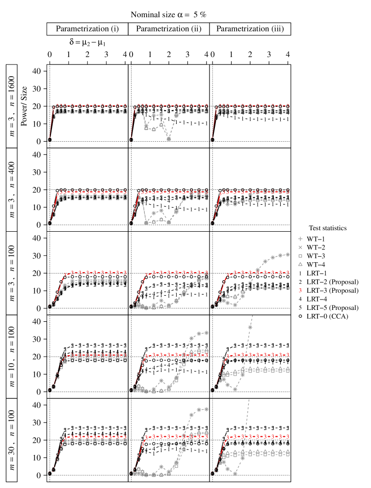
The power curves under nominal size $0.5\%$ and $5\%$ are shown in Figure 2 of the main text and Figure 10, respectively. Note that the trivial modifications LRT-2 of LRT-1 cannot retrieve all the power it should have. Tables 6 and 7 show the minimum and maximum of the empirical sizes over the three parametrizations considered in each test — and only one value is needed for those tests that are invariant to parametrization — when the nominal size is $0.5\%$ and $5\%$, respectively. We see the deviations from the nominal $\alpha$ can be noticeable, especially when $m=3$. To take that into account, we report the empirical size adjusted power, that is, $O={\rm power}/\widehat{\alpha}$, which also has the interpretation as (an approximated) posterior odds of $H_{1}$ to $H_{0}$ (Bayarri et al., 2016). Figures 11 and 12 plot the result for nominal size $0.5\%$ and $5\%$, respectively. Compared with the benchmark L-0, the odds $O$ of the proposed robust MI test (L-5) is closer to the nominal value $1/\alpha$ as $\delta\rightarrow\infty$. Nevertheless, the performances of all size $0.5\%$ tests are less satisfactory than those for size $5\%$ tests because larger sample sizes $n$ are required to approximate the tail behavior well.

Figure 11: The ratios of empirical power to empirical size under different parametrizations. The nominal size is $\alpha=0.5\%$. In each plot, the vertical axis denotes the ratio, and the horizontal axis denotes $\delta=\mu_{2}-\mu_{1}$. The legend in Figure 8 also applies here. The results under nominal size $5\%$ are shown in Figure 12.

Figure 12: The ratios of empirical power to empirical size under different parametrizations. The nominal size is $\alpha=5\%$. In each plot, the vertical axis denotes the ratio, whereas the horizontal axis denotes $\delta=\mu_{2}-\mu_{1}$. The legend in Figure 8 also applies here.

Table 6: The range of empirical size $[\min\widehat{\alpha},\max\widehat{\alpha}]$ in percentage, where $\max$ and $\min$ are taken over the three parametrizations. Only one value is recorded for parametrization-invariant tests. The nominal size is $\alpha=0.5\%$. The results under nominal size $\alpha=5\%$ are shown in Figure 7.

	Range of empirical size: $[\min\widehat{\alpha},\max\widehat{\alpha}]/\%$
$(n,m)$	$(1600,3)$	$(400,3)$	$(100,3)$	$(100,10)$	$(100,30)$
W-1	$[0.90,1.05]$	$[0.76,1.05]$	$[0.20,1.22]$	$[0.07,0.56]$	$[0.02,0.49]$
W-2	$[0.90,1.05]$	$[0.98,1.22]$	$[0.93,1.25]$	$[0.32,0.73]$	$[0.20,0.85]$
W-3	$[0.98,1.05]$	$[0.98,1.25]$	$[0.90,1.29]$	$[0.34,0.71]$	$[0.22,0.73]$
W-4	$[0.90,1.05]$	$[0.76,1.05]$	$[0.20,1.22]$	$[0.07,0.56]$	$[0.02,0.49]$
L-1	$[0.90,1.03]$	$[1.10,1.64]$	$[1.15,1.49]$	$[0.37,1.05]$	$[0.10,0.46]$
L-2	$[0.90,1.05]$	$[1.10,1.76]$	$[1.15,2.37]$	$[0.37,0.98]$	$[0.10,0.49]$
L-3	$0.90$	$1.10$	$0.83$	$0.24$	$0.07$
L-4	$0.90$	$1.10$	$0.83$	$0.24$	$0.07$
L-5	$0.46$	$0.44$	$0.68$	$0.46$	$0.42$
L-0	$0.39$	$0.66$	$0.66$	$0.66$	$0.66$

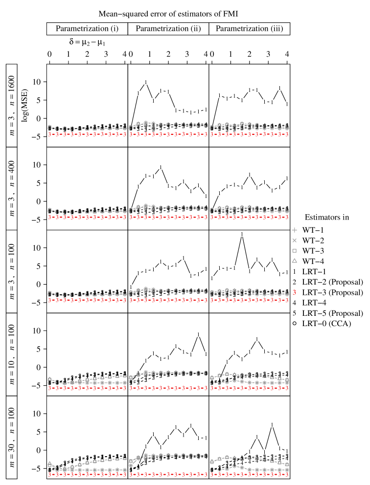
We also compare the performance of estimators of $\mathcal{r}_{m}$ for different $\delta$ and parametrizations. In our experiment, we have $\mathcal{r}_{m}=1+1/m$ because we have set $\mathcal{r}=1$. The MSEs of estimators $\widehat{f}=\widehat{r}/(1+\widehat{r})$ of $\mathcal{f}_{m}=\mathcal{r}_{m}/(1+\mathcal{r}_{m})$ are shown in Figure 13, in log scale. Clearly, the only estimator that is consistent, invariant to parametrization and robust against $\delta$ is our proposal $\widehat{f}_{\operatorname{L}}^{\operatorname{\lozenge}}=\widehat{r}_{\operatorname{L}}^{\operatorname{\lozenge}}/(1+\widehat{r}_{\operatorname{L}}^{\operatorname{\lozenge}})$. It concentrates at the true value $\mathcal{f}_{m}$ quite closely even for small $m$ and $n$. It verifies why L-5 has the greatest power. On the other hand, the estimator $\widetilde{f}_{\operatorname{L}}=\widetilde{r}_{\operatorname{L}}/(1+\widetilde{r}_{\operatorname{L}})$ has a large MSE when $\delta\not{=}0$. It explains why L-1 is not powerful.

Figure 13: The MSEs of estimators of $\mathcal{f}_{m}$ used in the test statistics. The vertical axis denotes the log of MSE, whereas the horizontal axis denotes the value of $\delta=\mu_{2}-\mu_{1}$. The legend in Figure 8 also applies here.

Table 7: The range of empirical size $[\min\widehat{\alpha},\max\widehat{\alpha}]$ in percentage, where $\max$ and $\min$ are taken over the three parametrizations. Only one value is recorded for parametrization-invariant tests. The nominal size is $\alpha=5\%$.

	Range of empirical size: $[\min\widehat{\alpha},\max\widehat{\alpha}]/\%$
$(n,m)$	$(1600,3)$	$(400,3)$	$(100,3)$	$(100,10)$	$(100,30)$
W-1	$[5.62,5.71]$	$[5.30,6.03]$	$[3.22,6.20]$	$[1.64,4.81]$	$[1.37,5.00]$
W-2	$[5.93,6.05]$	$[6.08,7.18]$	$[5.52,8.69]$	$[4.42,8.47]$	$[4.20,8.50]$
W-3	$[5.81,6.03]$	$[6.01,6.98]$	$[5.37,8.28]$	$[4.20,7.67]$	$[4.10,7.50]$
W-4	$[5.62,5.71]$	$[5.30,6.03]$	$[3.22,6.20]$	$[1.64,4.81]$	$[1.37,5.00]$
L-1	$[5.57,6.15]$	$[6.37,6.57]$	$[5.88,6.47]$	$[4.39,5.66]$	$[4.22,5.32]$
L-2	$[5.52,6.10]$	$[6.37,6.52]$	$[5.88,7.47]$	$[4.39,5.66]$	$[4.22,5.32]$
L-3	$5.76$	$6.37$	$5.42$	$3.78$	$3.71$
L-4	$5.76$	$6.37$	$5.42$	$3.78$	$3.71$
L-5	$4.96$	$5.32$	$4.93$	$4.79$	$4.54$
L-0	$5.03$	$5.03$	$5.57$	$5.57$	$5.57$

A.7 Supplements for Section 4.2

Let $n_{j}=\sum_{i=1}^{n}R_{ij}$ be the number of observed $j$th component. Without loss of generality, assume $X_{\operatorname{obs}}$ is arranged in such a way that $R_{ij}\geq R_{i^{\prime}j}$ for all $i<i^{\prime}$ and $j$. To impute the missing data, it is useful to represent $X_{i}$ by

$$\left[X_{i1}\mid\beta_{1},\tau_{1}^{2}\right]\sim\mathcal{N}(\beta_{1},\tau^{2}_{1})\qquad\text{and}\qquad\left[X_{ij}\mid X_{i,1:(j-1)},\beta_{j},\tau_{j}^{2}\right]\sim\mathcal{N}(\beta_{j}^{{\intercal}}Z_{ij},\tau^{2}_{j}),$$

for $j=2,\ldots,p$, where $\tau_{1}^{2},\ldots,\tau_{p}^{2}\in\mathbb{R}^{+}$, $\beta_{j}\in\mathbb{R}^{j}$, $X_{i,1:(j-1)}=(X_{i1},\ldots,X_{i,j-1})^{{\intercal}}$ and $Z_{ij}=(1,X_{i,1:(j-1)}^{{\intercal}})^{{\intercal}}$ for $j\geq 2$. Denote the (complete-case) least squares estimators of $\beta_{j}$ and $\tau^{2}_{j}$ respectively by

$$\widehat{\beta}_{j}=(Z_{j}^{{\intercal}}Z_{j})^{-1}Z_{j}^{{\intercal}}W_{j}\quad{\rm and}\quad\widehat{\tau}^{2}_{j}=\frac{(W_{j}-Z_{j}\widehat{\beta}_{j})^{{\intercal}}(W_{j}-Z_{j}\widehat{\beta}_{j})}{n_{j}-j},$$

where $Z_{j}=(Z_{1j},\ldots,Z_{n_{j}j})^{{\intercal}}$ and $W_{j}=(X_{1j},\ldots,X_{n_{j}j})^{{\intercal}}$.

We assume a Bayesian imputation model with the non-informative prior $f(\beta_{1},\ldots,\beta_{p},\tau^{2}_{1},\ldots,\tau^{2}_{p})\;\propto\;1/(\tau^{2}_{1}\cdots\tau^{2}_{p}).$ For $\ell=1,\ldots,m$, denote the $\ell$th imputed data set by $X^{(\ell)}$, whose $(i,j)$th element is $X_{ij}^{(\ell)}$. If $1\leq j\leq p$ and $i\leq n_{j}$, then $X_{ij}^{(\ell)}=X_{ij}$, otherwise $X_{ij}^{(\ell)}$ is filled in by recursing the following steps for $j=2,\ldots,p$.

1. Draw a sample $(\tau_{j}^{(\ell)})^{2}$ from $\widehat{\tau}^{2}_{j}(n_{j}-j)/\chi^{2}_{n_{j}-j}$.

2. Draw a sample $\beta_{j}^{(\ell)}$ from $\mathcal{N}_{j}(\widehat{\beta}_{j},(\tau_{j}^{(\ell)})^{2}(Z_{j}^{{\intercal}}Z_{j})^{-1})$.

3. Draw a sample $X_{ij}^{(\ell)}$ from $\mathcal{N}((\beta_{j}^{(\ell)})^{{\intercal}}Z_{ij}^{(\ell)},(\tau_{j}^{(\ell)})^{2})$ for $i=n_{j}+1,\ldots,n$, where $Z_{ij}^{(\ell)}=(1,(X_{i,1:(j-1)}^{(\ell)})^{{\intercal}})^{{\intercal}}$.

With the $\ell$th imputed data set, the $H_{0}$-constrained MLEs of $\mu$ and $\Sigma$ are $\widehat{\mu}_{0}^{(\ell)}=\bm{0}_{p}$ and $\widehat{\Sigma}_{0}^{(\ell)}=(X^{(\ell)})^{{\intercal}}(X^{(\ell)})/n$; whereas the unconstrained counterparts are $\widehat{\mu}^{(\ell)}=\bm{1}_{n}^{{\intercal}}X^{(\ell)}/n$ and $\widehat{\Sigma}^{(\ell)}=(X^{(\ell)}-\widehat{\mu}^{(\ell)})^{{\intercal}}(X^{(\ell)}-\widehat{\mu}^{(\ell)})/n$.

The partial result is shown in Figure 3 of the main text, whereas the full version is shown in Figure 14.

Figure 14: The empirical size, empirical power, and their ratio. The first row of plots show the empirical sizes. The size of the complete-case test (C2) under MAR is off the chart (always equals to one) because it is invalid. The second and third rows of plots show the powers and the power-to-size ratios, respectively, where the nominal size is $0.5\%$.

A.8 Applications to a Care-Survival Data

Meng and Rubin (1992) considered the data given in Table 8, where $i$, $j$ and $k$ index, respectively, amount of parental care (less or more, corresponding to $i=1,2$), and survival status (died or survived, corresponding to $j=1,2$), and clinic (A or B, corresponding to $k=1,2$). The label $k$ is missing for some observations. The missing mechanism was assumed to be ignorable. We consider two null hypotheses: ($H_{0}$) the clinic and parental care are conditionally independent given the survival status, and ($H_{0}^{\prime}$) all three variables are independent. It is remarked that testing the conditional independence model (i.e., $H_{0}$) is useful from a modeling perceptive. If $H_{0}$ cannot be rejected, then one may be tempted to adopt the more parsimonious null model (for the cell probabilities). The same model is also suggested in Little and Rubin (2002) and Meng and Rubin (1992).

Our aim is to investigate the impact on $\{\widetilde{D}_{\operatorname{S}},\widehat{D}_{\operatorname{S}}^{+},\widehat{D}^{\operatorname{\lozenge}}_{\operatorname{S}}\}$ by the parametrization of the cell probabilities

$$\pi_{ijk}=\mathsf{P}(\text{parental care}=i,\text{survival status}=j,\text{clinic label}=k)$$

for $i,j,k\in\{1,2\}$; and the impact on $\{\widetilde{r}_{\operatorname{L}},\widehat{r}^{+}_{\operatorname{S}},\widehat{r}^{\operatorname{\lozenge}}_{\operatorname{S}}\}$ under different null hypotheses. Here the full model parameter vector can be expressed as $\psi=(\pi_{111},\pi_{112},\pi_{121},\pi_{122},\pi_{211},\pi_{212},\pi_{221})^{{\intercal}}$. Since the restrictions imposed by $H_{0}$ are $\pi_{ijk}=(\pi_{1jk}+\pi_{2jk})(\pi_{ij1}+\pi_{ij2})$ for $j=1,2$, one may express the parameter of interest as $\theta=(\theta_{1},\theta_{2})^{{\intercal}}$, where $\theta_{j}=\pi_{ijk}-(\pi_{1jk}+\pi_{2jk})(\pi_{ij1}+\pi_{ij2})$ for $j=1,2$. Then $H_{0}$ can be equivalently stated as $\theta=\theta_{0}$, where $\theta_{0}=(0,0)^{{\intercal}}$. Similarly, the parameter of interest under $H_{0}^{\prime}$ can be defined.

Table 8: Data from Meng and Rubin (1992). The notation “?” indicates missing label.

Parental care ($i$)			Less		More
Survival Status ($j$)			Died	Survived	Died	Survived
Clinic Label ($k$)		A	3	176	4	293
		B	17	197	2	23
		?	10	150	5	90

The computation of the stacked MI estimators of $\{\pi_{ijk}\}$ is presented in A.8 of the Appendix. We consider three parametrizations: (i) $\psi_{ijk}=\pi_{ijk}$; (ii) $\psi_{ijk}=\log\{\pi_{ijk}/(1-\pi_{ijk})\}$; and (iii) $\psi_{ij1}=\pi_{ij1}$ and $\psi_{ij2}=\pi_{ij2}/\pi_{ij1}$. Denote the $p$-values of tests $\{\widetilde{D}_{\operatorname{L}},\widehat{D}_{\operatorname{S}}^{+},\widehat{D}^{\operatorname{\lozenge}}_{\operatorname{S}}\}$ by $\{\widetilde{p}_{\operatorname{L}},\widehat{p}_{\operatorname{S}}^{+},\widehat{p}^{\operatorname{\lozenge}}_{\operatorname{S}}\}$, respectively. The results are summarized in Table 9. Clearly, only $\widehat{r}_{\operatorname{S}},\widehat{r}_{\operatorname{\lozenge}},\widehat{D}_{\operatorname{S}}^{+},\widehat{D}^{\operatorname{\lozenge}}_{\operatorname{S}}$ are always non-negative and parametrization-invariant. Some of the values of $\widetilde{r}_{\operatorname{L}}$ and $\widetilde{D}_{\operatorname{L}}$ are negative, leading to the meaningless $\widetilde{p}_{\operatorname{L}}=1$. For testing $H_{0}$, we have $\widehat{D}_{\operatorname{S}}^{+}\approx\widehat{D}_{\operatorname{S}}^{\operatorname{\lozenge}}$. For testing $H_{0}^{\prime}$, $\widehat{D}_{\operatorname{S}}^{+}$ and $\widehat{D}_{\operatorname{S}}^{\operatorname{\lozenge}}$ are not very close to each other, but they both lead to essentially zero $p$-value. These results reconfirm the conclusions in Meng and Rubin (1992). Moreover, only $\widehat{r}_{\operatorname{S}}^{\operatorname{\lozenge}}$ does not change under different null hypotheses.

The MI data sets are generated from a Bayesian model in Section 4.2 of Meng and Rubin (1992). The $\ell$th imputed log-likelihood function is $\log f(X^{(\ell)}\mid\pi)=\sum_{c}n_{c}^{(\ell)}\log\pi_{c}$, where $X^{(\ell)}$ are the cell counts $n_{c}^{(\ell)}$ in the $\ell$th imputed data set. Hence the unconstrained MLE of $\pi_{c}$ is $\widehat{\pi}_{c}^{(\ell)}={n_{c}^{(\ell)}}/{n_{+}^{(\ell)}}$, where $n_{+}^{(\ell)}=\sum_{c}n_{c}^{(\ell)}$. Let $n_{c}^{+}=\sum_{\ell=1}^{m}n_{c}^{(\ell)}$. Consequently, the joint log-likelihood based on the stacked data is

$$\log f(X^{\operatorname{S}}\mid\pi)=\sum_{\ell=1}^{m}\sum_{c}n_{c}^{(\ell)}\log\pi_{c}=\sum_{c}n_{c}^{+}\log\pi_{c},$$ (A.14)

Thus the unconstrained MLE with respect to (A.14) is $\widehat{\pi}_{c}^{\operatorname{S}}={n_{c}^{+}}/{n_{+}^{+}}$, where $n_{+}^{+}=\sum_{c}n_{c}^{+}$. Similarly, we can find the constrained MLEs under a given null.

Table 9: The LRTs using $\widetilde{D}_{\operatorname{L}}$, $\widehat{D}_{\operatorname{S}}^{+}$ and $\widehat{D}^{\operatorname{\lozenge}}_{\operatorname{S}}$ under different parametrizations in Section A.8.

	Parametrization (i): identity map
	$H_{0}$: Conditional independence			$H_{0}$: Full independence
$m$	$\widetilde{r}_{\operatorname{L}},\widehat{r}^{+}_{\operatorname{S}},\widehat{r}^{\operatorname{\lozenge}}_{\operatorname{S}}$	$\widetilde{D}_{\operatorname{L}},\widehat{D}_{\operatorname{S}}^{+},\widehat{D}_{\operatorname{S}}^{\operatorname{\lozenge}}$	$\widetilde{p}_{\operatorname{L}},\widehat{p}_{\operatorname{S}}^{+},\widehat{p}_{\operatorname{S}}^{\operatorname{\lozenge}}$	$\widetilde{r}_{\operatorname{L}},\widehat{r}^{+}_{\operatorname{S}},\widehat{r}^{\operatorname{\lozenge}}_{\operatorname{S}}$	$\widetilde{D}_{\operatorname{L}},\widehat{D}_{\operatorname{S}}^{+},\widehat{D}_{\operatorname{S}}^{\operatorname{\lozenge}}$	$\widetilde{p}_{\operatorname{L}},\widehat{p}_{\operatorname{S}}^{+},\widehat{p}_{\operatorname{S}}^{\operatorname{\lozenge}}$
$2$	$0.63,0.64,0.83$	$0.14,0.14,0.12$	$0.87,0.87,0.89$	$0.53,0.53,0.83$	$44.4,44.4,37.1$	$0,0,0$
$3$	$0.54,0.54,0.38$	$0.08,0.08,0.09$	$0.93,0.93,0.92$	$0.31,0.31,0.38$	$54.2,54.2,51.4$	$0,0,0$
$5$	$0.49,0.48,0.89$	$0.12,0.12,0.10$	$0.89,0.89,0.91$	$0.72,0.72,0.89$	$40.8,40.8,37.1$	$0,0,0$
$7$	$0.23,0.23,0.47$	$0.06,0.06,0.05$	$0.94,0.94,0.95$	$0.31,0.31,0.47$	$53.2,53.2,47.6$	$0,0,0$
$10$	$0.50,0.50,0.70$	$0.14,0.14,0.12$	$0.87,0.87,0.88$	$0.56,0.56,0.70$	$45.4,45.4,41.7$	$0,0,0$
$25$	$0.35,0.35,0.47$	$0.06,0.06,0.06$	$0.94,0.94,0.95$	$0.35,0.35,0.47$	$51.4,51.4,47.0$	$0,0,0$
$50$	$0.31,0.31,0.45$	$0.11,0.11,0.10$	$0.90,0.90,0.91$	$0.33,0.33,0.45$	$51.5,51.5,47.3$	$0,0,0$
	Parametrization (ii): logit transformation
	$H_{0}$: Conditional independence			$H_{0}$: Full independence
$m$	$\widetilde{r}_{\operatorname{L}},\widehat{r}^{+}_{\operatorname{S}},\widehat{r}^{\operatorname{\lozenge}}_{\operatorname{S}}$	$\widetilde{D}_{\operatorname{L}},\widehat{D}_{\operatorname{S}}^{+},\widehat{D}_{\operatorname{S}}^{\operatorname{\lozenge}}$	$\widetilde{p}_{\operatorname{L}},\widehat{p}_{\operatorname{S}}^{+},\widehat{p}_{\operatorname{S}}^{\operatorname{\lozenge}}$	$\widetilde{r}_{\operatorname{L}},\widehat{r}^{+}_{\operatorname{S}},\widehat{r}^{\operatorname{\lozenge}}_{\operatorname{S}}$	$\widetilde{D}_{\operatorname{L}},\widehat{D}_{\operatorname{S}}^{+},\widehat{D}_{\operatorname{S}}^{\operatorname{\lozenge}}$	$\widetilde{p}_{\operatorname{L}},\widehat{p}_{\operatorname{S}}^{+},\widehat{p}_{\operatorname{S}}^{\operatorname{\lozenge}}$
$2$	$1.23,0.64,0.83$	$0.01,0.14,0.12$	$0.99,0.87,0.89$	$0.98,0.53,0.83$	$34.2,44.4,37.1$	$0,0,0$
$3$	$1.08,0.54,0.38$	$-0.07,0.08,0.09$	$1.00,0.93,0.92$	$0.61,0.31,0.38$	$43.9,54.2,51.4$	$0,0,0$
$5$	$1.02,0.48,0.89$	$-0.09,0.12,0.10$	$1.00,0.89,0.91$	$1.40,0.72,0.89$	$29.0,40.8,37.1$	$0,0,0$
$7$	$0.45,0.23,0.47$	$-0.07,0.06,0.05$	$1.00,0.94,0.95$	$0.58,0.31,0.47$	$43.9,53.2,47.6$	$0,0,0$
$10$	$0.99,0.50,0.70$	$-0.10,0.14,0.12$	$1.00,0.87,0.88$	$1.09,0.56,0.70$	$33.7,45.4,41.7$	$0,0,0$
$25$	$0.71,0.35,0.47$	$-0.14,0.06,0.06$	$1.00,0.94,0.95$	$0.68,0.35,0.47$	$41.0,51.4,47.0$	$0,0,0$
$50$	$0.63,0.31,0.45$	$-0.10,0.11,0.10$	$1.00,0.90,0.91$	$0.65,0.33,0.45$	$41.3,51.5,47.3$	$0,0,0$
	Parametrization (iii): ratios of probabilities
	$H_{0}$: Conditional independence			$H_{0}$: Full independence
$m$	$\widetilde{r}_{\operatorname{L}},\widehat{r}^{+}_{\operatorname{S}},\widehat{r}^{\operatorname{\lozenge}}_{\operatorname{S}}$	$\widetilde{D}_{\operatorname{L}},\widehat{D}_{\operatorname{S}}^{+},\widehat{D}_{\operatorname{S}}^{\operatorname{\lozenge}}$	$\widetilde{p}_{\operatorname{L}},\widehat{p}_{\operatorname{S}}^{+},\widehat{p}_{\operatorname{S}}^{\operatorname{\lozenge}}$	$\widetilde{r}_{\operatorname{L}},\widehat{r}^{+}_{\operatorname{S}},\widehat{r}^{\operatorname{\lozenge}}_{\operatorname{S}}$	$\widetilde{D}_{\operatorname{L}},\widehat{D}_{\operatorname{S}}^{+},\widehat{D}_{\operatorname{S}}^{\operatorname{\lozenge}}$	$\widetilde{p}_{\operatorname{L}},\widehat{p}_{\operatorname{S}}^{+},\widehat{p}_{\operatorname{S}}^{\operatorname{\lozenge}}$
$2$	$1.06,0.64,0.83$	$0.04,0.14,0.12$	$0.96,0.87,0.88$	$-0.38,0.53,0.83$	$109,44.4,37.1$	$0,0,0$
$3$	$-2.35,0.54,0.38$	$-1.16,0.08,0.09$	$1.00,0.93,0.92$	$-1.22,0.31,0.38$	$-321,54.2,51.4$	$1,0,0$
$5$	$-2.64,0.48,0.89$	$-1.38,0.12,0.10$	$1.00,0.89,0.91$	$-2.24,0.72,0.89$	$-58,40.8,37.1$	$1,0,0$
$7$	$-0.01,0.23,0.47$	$0.25,0.06,0.05$	$0.78,0.94,0.95$	$-0.34,0.31,0.47$	$107,53.2,47.6$	$0,0,0$
$10$	$-2.04,0.50,0.70$	$-2.20,0.14,0.12$	$1.00,0.87,0.88$	$-1.85,0.56,0.70$	$-86,45.4,41.7$	$1,0,0$
$25$	$-1.39,0.35,0.47$	$-4.30,0.06,0.06$	$1.00,0.94,0.95$	$-1.12,0.35,0.47$	$-603,51.4,47.0$	$1,0,0$
$50$	$-1.22,0.31,0.45$	$-7.39,0.11,0.10$	$1.00,0.90,0.91$	$-1.06,0.33,0.45$	$-1136,51.5,47.3$	$1,0,0$

Appendix B Proofs

Proof of Theorem 1.

(i, ii) From (2.3), we know $\widehat{d}_{\operatorname{L}}\geq 0$ is invariant to parametrization $\psi$. (iii) Since $\widehat{d}_{\operatorname{L}}$ is invariant to transformation of $\psi$, we assume, without loss of generality, that $\psi$ admits a parameterization such that $\operatorname{\textnormal{Cov}}(\widehat{\theta}^{(\ell)},\widehat{\eta}^{(\ell)})\bumpeq\mathbf{0}$ by taking suitable linear transformation of $\psi$. Also write $U^{(\ell)}_{\eta}$ as an efficient estimator of $\operatorname{\textnormal{Var}}(\widehat{\eta})$ based on $X^{(\ell)}$; and recall that $U^{(\ell)}_{\theta}=U^{(\ell)}$ is an efficient estimator of $\operatorname{\textnormal{Var}}(\widehat{\theta})$ based on $X^{(\ell)}$.

Using Taylor’s expansion on $\psi\mapsto\overline{L}(\psi)=m^{-1}\sum_{\ell=1}^{m}\log f(X^{(\ell)}\mid\psi)$ around $\widehat{\psi}^{*}=((\widehat{\theta}^{*})^{{\intercal}},(\widehat{\eta}^{*})^{{\intercal}})^{{\intercal}}$, we know that for $\psi\bumpeq\widehat{\psi}^{*}$,

$$\overline{L}(\psi)\bumpeq\overline{L}(\widehat{\psi}^{*})-\frac{1}{2}\left(\psi-\widehat{\psi}^{*}\right)^{{\intercal}}\overline{I}(\widehat{\psi}^{*})\left(\psi-\widehat{\psi}^{*}\right),$$ (B.1)

where $\overline{I}(\psi)=-{\partial^{2}\overline{L}(\psi)}/{\partial\psi\partial\psi^{{\intercal}}}$, which satisfies

$$\overline{I}(\widehat{\psi}^{*})\bumpeq\left(\begin{array}[]{cc}\overline{U}^{-1}_{\theta}&\mathbf{0}\\ \mathbf{0}&\overline{U}^{-1}_{\eta}\end{array}\right)$$ (B.2)

with $\overline{U}_{\eta}=m^{-1}\sum_{i=1}^{m}U^{(\ell)}_{\eta}$. Under the null, $\widehat{\psi}^{*}\bumpeq\widehat{\psi}_{0}^{*}$. So, using (B.1), we have

$$\widehat{d}_{\operatorname{L}} \bumpeq \left(\widehat{\psi}_{0}^{*}-\widehat{\psi}^{*}\right)^{{\intercal}}\overline{I}(\widehat{\psi}^{*})\left(\widehat{\psi}_{0}^{*}-\widehat{\psi}^{*}\right),$$ (B.9)

$$\bumpeq \left(\begin{array}[]{c}\theta_{0}-\widehat{\theta}^{*}\\ \widehat{\eta}(\theta_{0})-\widehat{\eta}(\widehat{\theta}^{*})\end{array}\right)^{{\intercal}}\left(\begin{array}[]{cc}\overline{U}^{-1}_{\theta}&\mathbf{0}\\ \mathbf{0}&\overline{U}^{-1}_{\eta}\end{array}\right)\left(\begin{array}[]{c}\theta_{0}-\widehat{\theta}^{*}\\ \widehat{\eta}(\theta_{0})-\widehat{\eta}(\widehat{\theta}^{*})\end{array}\right)$$

$$\bumpeq (\overline{\theta}^{{\intercal}}-\theta_{0})\overline{U}^{-1}_{\theta}(\overline{\theta}^{{\intercal}}-\theta_{0})=\widetilde{d}_{\operatorname{W}}^{\prime},$$ (B.10)

where we have used (a) $\widehat{\theta}^{*}\bumpeq\overline{\theta}$; see, e.g., Lemma 1 of Wang and Robins (1998), and (b) $\widehat{\eta}(\theta_{0})-\widehat{\eta}(\widehat{\theta}^{*})=O_{p}(1/n)$ if $\theta_{0}-\widehat{\theta}^{*}=O_{p}(1/\sqrt{n})$; see Cox and Reid (1987). Since $\widetilde{d}_{\operatorname{W}}^{\prime}\bumpeq\widetilde{d}_{\operatorname{L}}$ (Meng and Rubin, 1992), we have $\widehat{d}_{\operatorname{L}}\bumpeq\widetilde{d}_{\operatorname{L}}$. ∎

Proof of Proposition 1.

The given condition implies that

$$\widehat{\psi}^{(\ell)}=((\widehat{\theta}^{(\ell)})^{{\intercal}},(\widehat{\eta}^{(\ell)})^{{\intercal}})^{{\intercal}},\qquad\widehat{\psi}_{0}^{(\ell)}=(\theta_{0}^{{\intercal}},(\widehat{\eta}^{(\ell)})^{{\intercal}})^{{\intercal}},$$

$$\widehat{\psi}^{*}=((\widehat{\theta}^{*})^{{\intercal}},(\widehat{\eta}^{*})^{{\intercal}})^{{\intercal}},\qquad\widehat{\psi}_{0}^{*}=(\theta_{0}^{{\intercal}},(\widehat{\eta}^{*})^{{\intercal}})^{{\intercal}}.$$

Clearly, we also have the decomposition: $L^{(\ell)}(\psi)=L^{(\ell)}_{{\dagger}}(\theta)+L^{(\ell)}_{{\ddagger}}(\eta)$ for all $\ell$, where $L^{(\ell)}_{{\dagger}}(\theta)=L_{{\dagger}}(\theta\mid X^{(\ell)})$ and $L^{(\ell)}_{{\ddagger}}(\eta)=L_{{\ddagger}}(\eta\mid X^{(\ell)})$. Then,

$$\overline{d}_{\operatorname{L}}-\widehat{d}_{\operatorname{L}} = \frac{2}{m}\sum_{\ell=1}^{m}\left\{L^{(\ell)}(\widehat{\psi}^{(\ell)})-L^{(\ell)}(\widehat{\psi}_{0}^{(\ell)})-L^{(\ell)}(\widehat{\psi}^{*})+L^{(\ell)}(\widehat{\psi}_{0}^{*})\right\}$$

$$= \frac{2}{m}\sum_{\ell=1}^{m}\left\{L^{(\ell)}_{{\dagger}}(\widehat{\theta}^{(\ell)})-L_{{\dagger}}^{(\ell)}(\widehat{\theta}^{*})\right\}\geq 0$$

since $L^{(\ell)}_{{\dagger}}(\widehat{\theta}^{(\ell)})\geq L_{{\dagger}}^{(\ell)}(\widehat{\theta}^{*})$ for all $\ell$. ∎

Proof of Corollary 1.

Applying Taylor’s expansion on $\psi\mapsto L^{(\ell)}(\psi)$, we can find ${\mathchoice{{\ooalign{\hbox{\raise 7.12962pt\hbox{\scalebox{1.0}[-1.0]{\lower 7.12962pt\hbox{$\displaystyle\widehat{\vrule width=0.0pt,height=6.94444pt\vrule height=0.0pt,width=6.51392pt}$}}}}\cr\hbox{$\displaystyle\psi$}}}}{{\ooalign{\hbox{\raise 7.12962pt\hbox{\scalebox{1.0}[-1.0]{\lower 7.12962pt\hbox{$\textstyle\widehat{\vrule width=0.0pt,height=6.94444pt\vrule height=0.0pt,width=6.51392pt}$}}}}\cr\hbox{$\textstyle\psi$}}}}{{\ooalign{\hbox{\raise 6.43518pt\hbox{\scalebox{1.0}[-1.0]{\lower 6.43518pt\hbox{$\scriptstyle\widehat{\vrule width=0.0pt,height=4.8611pt\vrule height=0.0pt,width=4.55974pt}$}}}}\cr\hbox{$\scriptstyle\psi$}}}}{{\ooalign{\hbox{\raise 5.97221pt\hbox{\scalebox{1.0}[-1.0]{\lower 5.97221pt\hbox{$\scriptscriptstyle\widehat{\vrule width=0.0pt,height=3.47221pt\vrule height=0.0pt,width=3.25696pt}$}}}}\cr\hbox{$\scriptscriptstyle\psi$}}}}}{}^{(\ell)}$ lying on the line segment joining $\widehat{\psi}^{(\ell)}$ and $\widehat{\psi}_{0}^{(\ell)}$ such that

$$L^{(\ell)}(\widehat{\psi}_{0}^{(\ell)})=L^{(\ell)}(\widehat{\psi}^{(\ell)})-\frac{1}{2}\left(\widehat{\psi}_{0}^{(\ell)}-\widehat{\psi}^{(\ell)}\right)^{{\intercal}}I^{(\ell)}({\mathchoice{{\ooalign{\hbox{\raise 7.12962pt\hbox{\scalebox{1.0}[-1.0]{\lower 7.12962pt\hbox{$\displaystyle\widehat{\vrule width=0.0pt,height=6.94444pt\vrule height=0.0pt,width=6.51392pt}$}}}}\cr\hbox{$\displaystyle\psi$}}}}{{\ooalign{\hbox{\raise 7.12962pt\hbox{\scalebox{1.0}[-1.0]{\lower 7.12962pt\hbox{$\textstyle\widehat{\vrule width=0.0pt,height=6.94444pt\vrule height=0.0pt,width=6.51392pt}$}}}}\cr\hbox{$\textstyle\psi$}}}}{{\ooalign{\hbox{\raise 6.43518pt\hbox{\scalebox{1.0}[-1.0]{\lower 6.43518pt\hbox{$\scriptstyle\widehat{\vrule width=0.0pt,height=4.8611pt\vrule height=0.0pt,width=4.55974pt}$}}}}\cr\hbox{$\scriptstyle\psi$}}}}{{\ooalign{\hbox{\raise 5.97221pt\hbox{\scalebox{1.0}[-1.0]{\lower 5.97221pt\hbox{$\scriptscriptstyle\widehat{\vrule width=0.0pt,height=3.47221pt\vrule height=0.0pt,width=3.25696pt}$}}}}\cr\hbox{$\scriptscriptstyle\psi$}}}}}{}^{(\ell)})\left(\widehat{\psi}_{0}^{(\ell)}-\widehat{\psi}^{(\ell)}\right),$$

where $I^{(\ell)}(\psi)=-\partial^{2}L^{(\ell)}(\psi)/\partial\psi\partial\psi^{{\intercal}}$. By the lower order variability of $I^{(\ell)}({\mathchoice{{\ooalign{\hbox{\raise 7.12962pt\hbox{\scalebox{1.0}[-1.0]{\lower 7.12962pt\hbox{$\displaystyle\widehat{\vrule width=0.0pt,height=6.94444pt\vrule height=0.0pt,width=6.51392pt}$}}}}\cr\hbox{$\displaystyle\psi$}}}}{{\ooalign{\hbox{\raise 7.12962pt\hbox{\scalebox{1.0}[-1.0]{\lower 7.12962pt\hbox{$\textstyle\widehat{\vrule width=0.0pt,height=6.94444pt\vrule height=0.0pt,width=6.51392pt}$}}}}\cr\hbox{$\textstyle\psi$}}}}{{\ooalign{\hbox{\raise 6.43518pt\hbox{\scalebox{1.0}[-1.0]{\lower 6.43518pt\hbox{$\scriptstyle\widehat{\vrule width=0.0pt,height=4.8611pt\vrule height=0.0pt,width=4.55974pt}$}}}}\cr\hbox{$\scriptstyle\psi$}}}}{{\ooalign{\hbox{\raise 5.97221pt\hbox{\scalebox{1.0}[-1.0]{\lower 5.97221pt\hbox{$\scriptscriptstyle\widehat{\vrule width=0.0pt,height=3.47221pt\vrule height=0.0pt,width=3.25696pt}$}}}}\cr\hbox{$\scriptscriptstyle\psi$}}}}}{}^{(\ell)})$, we can find ${\mathchoice{{\ooalign{\hbox{\raise 7.12962pt\hbox{\scalebox{1.0}[-1.0]{\lower 7.12962pt\hbox{$\displaystyle\widehat{\vrule width=0.0pt,height=6.94444pt\vrule height=0.0pt,width=6.51392pt}$}}}}\cr\hbox{$\displaystyle\psi$}}}}{{\ooalign{\hbox{\raise 7.12962pt\hbox{\scalebox{1.0}[-1.0]{\lower 7.12962pt\hbox{$\textstyle\widehat{\vrule width=0.0pt,height=6.94444pt\vrule height=0.0pt,width=6.51392pt}$}}}}\cr\hbox{$\textstyle\psi$}}}}{{\ooalign{\hbox{\raise 6.43518pt\hbox{\scalebox{1.0}[-1.0]{\lower 6.43518pt\hbox{$\scriptstyle\widehat{\vrule width=0.0pt,height=4.8611pt\vrule height=0.0pt,width=4.55974pt}$}}}}\cr\hbox{$\scriptstyle\psi$}}}}{{\ooalign{\hbox{\raise 5.97221pt\hbox{\scalebox{1.0}[-1.0]{\lower 5.97221pt\hbox{$\scriptscriptstyle\widehat{\vrule width=0.0pt,height=3.47221pt\vrule height=0.0pt,width=3.25696pt}$}}}}\cr\hbox{$\scriptscriptstyle\psi$}}}}}{}^{*}$ such that $I^{(\ell)}({\mathchoice{{\ooalign{\hbox{\raise 7.12962pt\hbox{\scalebox{1.0}[-1.0]{\lower 7.12962pt\hbox{$\displaystyle\widehat{\vrule width=0.0pt,height=6.94444pt\vrule height=0.0pt,width=6.51392pt}$}}}}\cr\hbox{$\displaystyle\psi$}}}}{{\ooalign{\hbox{\raise 7.12962pt\hbox{\scalebox{1.0}[-1.0]{\lower 7.12962pt\hbox{$\textstyle\widehat{\vrule width=0.0pt,height=6.94444pt\vrule height=0.0pt,width=6.51392pt}$}}}}\cr\hbox{$\textstyle\psi$}}}}{{\ooalign{\hbox{\raise 6.43518pt\hbox{\scalebox{1.0}[-1.0]{\lower 6.43518pt\hbox{$\scriptstyle\widehat{\vrule width=0.0pt,height=4.8611pt\vrule height=0.0pt,width=4.55974pt}$}}}}\cr\hbox{$\scriptstyle\psi$}}}}{{\ooalign{\hbox{\raise 5.97221pt\hbox{\scalebox{1.0}[-1.0]{\lower 5.97221pt\hbox{$\scriptscriptstyle\widehat{\vrule width=0.0pt,height=3.47221pt\vrule height=0.0pt,width=3.25696pt}$}}}}\cr\hbox{$\scriptscriptstyle\psi$}}}}}{}^{(\ell)})\bumpeq I^{(\ell)}({\mathchoice{{\ooalign{\hbox{\raise 7.12962pt\hbox{\scalebox{1.0}[-1.0]{\lower 7.12962pt\hbox{$\displaystyle\widehat{\vrule width=0.0pt,height=6.94444pt\vrule height=0.0pt,width=6.51392pt}$}}}}\cr\hbox{$\displaystyle\psi$}}}}{{\ooalign{\hbox{\raise 7.12962pt\hbox{\scalebox{1.0}[-1.0]{\lower 7.12962pt\hbox{$\textstyle\widehat{\vrule width=0.0pt,height=6.94444pt\vrule height=0.0pt,width=6.51392pt}$}}}}\cr\hbox{$\textstyle\psi$}}}}{{\ooalign{\hbox{\raise 6.43518pt\hbox{\scalebox{1.0}[-1.0]{\lower 6.43518pt\hbox{$\scriptstyle\widehat{\vrule width=0.0pt,height=4.8611pt\vrule height=0.0pt,width=4.55974pt}$}}}}\cr\hbox{$\scriptstyle\psi$}}}}{{\ooalign{\hbox{\raise 5.97221pt\hbox{\scalebox{1.0}[-1.0]{\lower 5.97221pt\hbox{$\scriptscriptstyle\widehat{\vrule width=0.0pt,height=3.47221pt\vrule height=0.0pt,width=3.25696pt}$}}}}\cr\hbox{$\scriptscriptstyle\psi$}}}}}{}^{*})$ for all $\ell$. Then, using similar techniques as in (B.2) and (B.9), we have

$$L^{(\ell)}(\widehat{\psi}^{(\ell)})-L^{(\ell)}(\widehat{\psi}_{0}^{(\ell)}) \bumpeq \frac{1}{2}\left(\widehat{\psi}_{0}^{(\ell)}-\widehat{\psi}^{(\ell)}\right)^{{\intercal}}I^{(\ell)}({\mathchoice{{\ooalign{\hbox{\raise 7.12962pt\hbox{\scalebox{1.0}[-1.0]{\lower 7.12962pt\hbox{$\displaystyle\widehat{\vrule width=0.0pt,height=6.94444pt\vrule height=0.0pt,width=6.51392pt}$}}}}\cr\hbox{$\displaystyle\psi$}}}}{{\ooalign{\hbox{\raise 7.12962pt\hbox{\scalebox{1.0}[-1.0]{\lower 7.12962pt\hbox{$\textstyle\widehat{\vrule width=0.0pt,height=6.94444pt\vrule height=0.0pt,width=6.51392pt}$}}}}\cr\hbox{$\textstyle\psi$}}}}{{\ooalign{\hbox{\raise 6.43518pt\hbox{\scalebox{1.0}[-1.0]{\lower 6.43518pt\hbox{$\scriptstyle\widehat{\vrule width=0.0pt,height=4.8611pt\vrule height=0.0pt,width=4.55974pt}$}}}}\cr\hbox{$\scriptstyle\psi$}}}}{{\ooalign{\hbox{\raise 5.97221pt\hbox{\scalebox{1.0}[-1.0]{\lower 5.97221pt\hbox{$\scriptscriptstyle\widehat{\vrule width=0.0pt,height=3.47221pt\vrule height=0.0pt,width=3.25696pt}$}}}}\cr\hbox{$\scriptscriptstyle\psi$}}}}}{}^{*})\left(\widehat{\psi}_{0}^{(\ell)}-\widehat{\psi}^{(\ell)}\right)$$ (B.19)

$$\bumpeq \frac{1}{2}\left(\theta_{0}-\widehat{\theta}^{(\ell)}\right)^{{\intercal}}{\mathchoice{{\ooalign{\hbox{\raise 7.09259pt\hbox{\scalebox{1.0}[-1.0]{\lower 7.09259pt\hbox{$\displaystyle\widehat{\vrule width=0.0pt,height=6.83331pt\vrule height=0.0pt,width=7.91803pt}$}}}}\cr\hbox{$\displaystyle U$}}}}{{\ooalign{\hbox{\raise 7.09259pt\hbox{\scalebox{1.0}[-1.0]{\lower 7.09259pt\hbox{$\textstyle\widehat{\vrule width=0.0pt,height=6.83331pt\vrule height=0.0pt,width=7.91803pt}$}}}}\cr\hbox{$\textstyle U$}}}}{{\ooalign{\hbox{\raise 6.40926pt\hbox{\scalebox{1.0}[-1.0]{\lower 6.40926pt\hbox{$\scriptstyle\widehat{\vrule width=0.0pt,height=4.78333pt\vrule height=0.0pt,width=5.54262pt}$}}}}\cr\hbox{$\scriptstyle U$}}}}{{\ooalign{\hbox{\raise 5.9537pt\hbox{\scalebox{1.0}[-1.0]{\lower 5.9537pt\hbox{$\scriptscriptstyle\widehat{\vrule width=0.0pt,height=3.41666pt\vrule height=0.0pt,width=3.959pt}$}}}}\cr\hbox{$\scriptscriptstyle U$}}}}}^{-1}\left(\theta_{0}-\widehat{\theta}^{(\ell)}\right)$$ (B.28)

for some matrix $\textstyle\widehat{\vrule width=0.0pt,height=6.83331pt\vrule height=0.0pt,width=7.91803pt}$ $\textstyle U$ . Similarly, we have

$$L^{(\ell)}(\widehat{\psi}^{*})-L^{(\ell)}(\widehat{\psi}_{0}^{*})\bumpeq\frac{1}{2}\left(\theta_{0}-\widehat{\theta}^{*}\right)^{{\intercal}}{\mathchoice{{\ooalign{\hbox{\raise 7.09259pt\hbox{\scalebox{1.0}[-1.0]{\lower 7.09259pt\hbox{$\displaystyle\widehat{\vrule width=0.0pt,height=6.83331pt\vrule height=0.0pt,width=7.91803pt}$}}}}\cr\hbox{$\displaystyle U$}}}}{{\ooalign{\hbox{\raise 7.09259pt\hbox{\scalebox{1.0}[-1.0]{\lower 7.09259pt\hbox{$\textstyle\widehat{\vrule width=0.0pt,height=6.83331pt\vrule height=0.0pt,width=7.91803pt}$}}}}\cr\hbox{$\textstyle U$}}}}{{\ooalign{\hbox{\raise 6.40926pt\hbox{\scalebox{1.0}[-1.0]{\lower 6.40926pt\hbox{$\scriptstyle\widehat{\vrule width=0.0pt,height=4.78333pt\vrule height=0.0pt,width=5.54262pt}$}}}}\cr\hbox{$\scriptstyle U$}}}}{{\ooalign{\hbox{\raise 5.9537pt\hbox{\scalebox{1.0}[-1.0]{\lower 5.9537pt\hbox{$\scriptscriptstyle\widehat{\vrule width=0.0pt,height=3.41666pt\vrule height=0.0pt,width=3.959pt}$}}}}\cr\hbox{$\scriptscriptstyle U$}}}}}^{-1}\left(\theta_{0}-\widehat{\theta}^{*}\right).$$ (B.29)

Write $A^{\otimes 2}=AA^{{\intercal}}$ for any appropriate matrix $A$. Using (B.19), (B.29) and the cyclic property of trace, we have

$$\overline{d}_{\operatorname{L}}-\widehat{d}_{\operatorname{L}} \bumpeq \frac{1}{m}\sum_{\ell=1}^{m}\left\{\left(\theta_{0}-\widehat{\theta}^{(\ell)}\right)^{{\intercal}}{\mathchoice{{\ooalign{\hbox{\raise 7.09259pt\hbox{\scalebox{1.0}[-1.0]{\lower 7.09259pt\hbox{$\displaystyle\widehat{\vrule width=0.0pt,height=6.83331pt\vrule height=0.0pt,width=7.91803pt}$}}}}\cr\hbox{$\displaystyle U$}}}}{{\ooalign{\hbox{\raise 7.09259pt\hbox{\scalebox{1.0}[-1.0]{\lower 7.09259pt\hbox{$\textstyle\widehat{\vrule width=0.0pt,height=6.83331pt\vrule height=0.0pt,width=7.91803pt}$}}}}\cr\hbox{$\textstyle U$}}}}{{\ooalign{\hbox{\raise 6.40926pt\hbox{\scalebox{1.0}[-1.0]{\lower 6.40926pt\hbox{$\scriptstyle\widehat{\vrule width=0.0pt,height=4.78333pt\vrule height=0.0pt,width=5.54262pt}$}}}}\cr\hbox{$\scriptstyle U$}}}}{{\ooalign{\hbox{\raise 5.9537pt\hbox{\scalebox{1.0}[-1.0]{\lower 5.9537pt\hbox{$\scriptscriptstyle\widehat{\vrule width=0.0pt,height=3.41666pt\vrule height=0.0pt,width=3.959pt}$}}}}\cr\hbox{$\scriptscriptstyle U$}}}}}^{-1}\left(\theta_{0}-\widehat{\theta}^{(\ell)}\right)-\left(\theta_{0}-\widehat{\theta}^{*}\right)^{{\intercal}}{\mathchoice{{\ooalign{\hbox{\raise 7.09259pt\hbox{\scalebox{1.0}[-1.0]{\lower 7.09259pt\hbox{$\displaystyle\widehat{\vrule width=0.0pt,height=6.83331pt\vrule height=0.0pt,width=7.91803pt}$}}}}\cr\hbox{$\displaystyle U$}}}}{{\ooalign{\hbox{\raise 7.09259pt\hbox{\scalebox{1.0}[-1.0]{\lower 7.09259pt\hbox{$\textstyle\widehat{\vrule width=0.0pt,height=6.83331pt\vrule height=0.0pt,width=7.91803pt}$}}}}\cr\hbox{$\textstyle U$}}}}{{\ooalign{\hbox{\raise 6.40926pt\hbox{\scalebox{1.0}[-1.0]{\lower 6.40926pt\hbox{$\scriptstyle\widehat{\vrule width=0.0pt,height=4.78333pt\vrule height=0.0pt,width=5.54262pt}$}}}}\cr\hbox{$\scriptstyle U$}}}}{{\ooalign{\hbox{\raise 5.9537pt\hbox{\scalebox{1.0}[-1.0]{\lower 5.9537pt\hbox{$\scriptscriptstyle\widehat{\vrule width=0.0pt,height=3.41666pt\vrule height=0.0pt,width=3.959pt}$}}}}\cr\hbox{$\scriptscriptstyle U$}}}}}^{-1}\left(\theta_{0}-\widehat{\theta}^{*}\right)\right\}$$

$$= \operatorname{tr}\left[{\mathchoice{{\ooalign{\hbox{\raise 7.09259pt\hbox{\scalebox{1.0}[-1.0]{\lower 7.09259pt\hbox{$\displaystyle\widehat{\vrule width=0.0pt,height=6.83331pt\vrule height=0.0pt,width=7.91803pt}$}}}}\cr\hbox{$\displaystyle U$}}}}{{\ooalign{\hbox{\raise 7.09259pt\hbox{\scalebox{1.0}[-1.0]{\lower 7.09259pt\hbox{$\textstyle\widehat{\vrule width=0.0pt,height=6.83331pt\vrule height=0.0pt,width=7.91803pt}$}}}}\cr\hbox{$\textstyle U$}}}}{{\ooalign{\hbox{\raise 6.40926pt\hbox{\scalebox{1.0}[-1.0]{\lower 6.40926pt\hbox{$\scriptstyle\widehat{\vrule width=0.0pt,height=4.78333pt\vrule height=0.0pt,width=5.54262pt}$}}}}\cr\hbox{$\scriptstyle U$}}}}{{\ooalign{\hbox{\raise 5.9537pt\hbox{\scalebox{1.0}[-1.0]{\lower 5.9537pt\hbox{$\scriptscriptstyle\widehat{\vrule width=0.0pt,height=3.41666pt\vrule height=0.0pt,width=3.959pt}$}}}}\cr\hbox{$\scriptscriptstyle U$}}}}}^{-1}\left\{\frac{1}{m}\sum_{\ell=1}^{m}\left(\theta_{0}-\widehat{\theta}^{(\ell)}\right)^{\otimes 2}-\left(\theta_{0}-\widehat{\theta}^{*}\right)^{\otimes 2}\right\}\right]$$

$$\bumpeq \operatorname{tr}\left[{\mathchoice{{\ooalign{\hbox{\raise 7.09259pt\hbox{\scalebox{1.0}[-1.0]{\lower 7.09259pt\hbox{$\displaystyle\widehat{\vrule width=0.0pt,height=6.83331pt\vrule height=0.0pt,width=7.91803pt}$}}}}\cr\hbox{$\displaystyle U$}}}}{{\ooalign{\hbox{\raise 7.09259pt\hbox{\scalebox{1.0}[-1.0]{\lower 7.09259pt\hbox{$\textstyle\widehat{\vrule width=0.0pt,height=6.83331pt\vrule height=0.0pt,width=7.91803pt}$}}}}\cr\hbox{$\textstyle U$}}}}{{\ooalign{\hbox{\raise 6.40926pt\hbox{\scalebox{1.0}[-1.0]{\lower 6.40926pt\hbox{$\scriptstyle\widehat{\vrule width=0.0pt,height=4.78333pt\vrule height=0.0pt,width=5.54262pt}$}}}}\cr\hbox{$\scriptstyle U$}}}}{{\ooalign{\hbox{\raise 5.9537pt\hbox{\scalebox{1.0}[-1.0]{\lower 5.9537pt\hbox{$\scriptscriptstyle\widehat{\vrule width=0.0pt,height=3.41666pt\vrule height=0.0pt,width=3.959pt}$}}}}\cr\hbox{$\scriptscriptstyle U$}}}}}^{-1}\frac{1}{m}\sum_{\ell=1}^{m}\left\{(\widehat{\theta}^{(\ell)})^{\otimes 2}-\overline{\theta}^{\otimes 2}\right\}\right]\bumpeq\operatorname{tr}\left({\mathchoice{{\ooalign{\hbox{\raise 7.09259pt\hbox{\scalebox{1.0}[-1.0]{\lower 7.09259pt\hbox{$\displaystyle\widehat{\vrule width=0.0pt,height=6.83331pt\vrule height=0.0pt,width=7.91803pt}$}}}}\cr\hbox{$\displaystyle U$}}}}{{\ooalign{\hbox{\raise 7.09259pt\hbox{\scalebox{1.0}[-1.0]{\lower 7.09259pt\hbox{$\textstyle\widehat{\vrule width=0.0pt,height=6.83331pt\vrule height=0.0pt,width=7.91803pt}$}}}}\cr\hbox{$\textstyle U$}}}}{{\ooalign{\hbox{\raise 6.40926pt\hbox{\scalebox{1.0}[-1.0]{\lower 6.40926pt\hbox{$\scriptstyle\widehat{\vrule width=0.0pt,height=4.78333pt\vrule height=0.0pt,width=5.54262pt}$}}}}\cr\hbox{$\scriptstyle U$}}}}{{\ooalign{\hbox{\raise 5.9537pt\hbox{\scalebox{1.0}[-1.0]{\lower 5.9537pt\hbox{$\scriptscriptstyle\widehat{\vrule width=0.0pt,height=3.41666pt\vrule height=0.0pt,width=3.959pt}$}}}}\cr\hbox{$\scriptscriptstyle U$}}}}}^{-1}B\right)\bumpeq\operatorname{tr}\left(\mathcal{U}_{\theta,0}^{-1}\mathcal{B}_{\theta}\right)$$

as $m,n\rightarrow\infty$, where $\mathcal{U}_{\theta,0}$ is a deterministic matrix that depends on both $\theta_{0}$ and the true value of $\theta$, and satisfies $n({\mathchoice{{\ooalign{\hbox{\raise 7.09259pt\hbox{\scalebox{1.0}[-1.0]{\lower 7.09259pt\hbox{$\displaystyle\widehat{\vrule width=0.0pt,height=6.83331pt\vrule height=0.0pt,width=7.91803pt}$}}}}\cr\hbox{$\displaystyle U$}}}}{{\ooalign{\hbox{\raise 7.09259pt\hbox{\scalebox{1.0}[-1.0]{\lower 7.09259pt\hbox{$\textstyle\widehat{\vrule width=0.0pt,height=6.83331pt\vrule height=0.0pt,width=7.91803pt}$}}}}\cr\hbox{$\textstyle U$}}}}{{\ooalign{\hbox{\raise 6.40926pt\hbox{\scalebox{1.0}[-1.0]{\lower 6.40926pt\hbox{$\scriptstyle\widehat{\vrule width=0.0pt,height=4.78333pt\vrule height=0.0pt,width=5.54262pt}$}}}}\cr\hbox{$\scriptstyle U$}}}}{{\ooalign{\hbox{\raise 5.9537pt\hbox{\scalebox{1.0}[-1.0]{\lower 5.9537pt\hbox{$\scriptscriptstyle\widehat{\vrule width=0.0pt,height=3.41666pt\vrule height=0.0pt,width=3.959pt}$}}}}\cr\hbox{$\scriptscriptstyle U$}}}}}-\mathcal{U}_{\theta,0})\overset{\mathrm{pr}}{\rightarrow}0$. Note that $\operatorname{tr}(\mathcal{U}_{\theta,0}^{-1}\mathcal{B}_{\theta})=k\mathcal{r}_{0}$, for some finite $\mathcal{r}_{0}$ by Assumption 2. Then $\widehat{r}_{\operatorname{L}}\overset{\mathrm{pr}}{\rightarrow}\mathcal{r}_{0}=\operatorname{tr}(\mathcal{U}_{\theta,0}^{-1}\mathcal{B}_{\theta})/k$, proving (ii). (But $\mathcal{U}_{\theta,0}$ may not equal to $\mathcal{U}_{\theta}$, and hence $\widehat{r}_{\operatorname{L}}$ may not be consistent for $\mathcal{r}_{m}$.)

If $H_{0}$ is true, then $\overline{\theta}\overset{\mathrm{pr}}{\rightarrow}\theta_{0}$ and ${\mathchoice{{\ooalign{\hbox{\raise 7.09259pt\hbox{\scalebox{1.0}[-1.0]{\lower 7.09259pt\hbox{$\displaystyle\widehat{\vrule width=0.0pt,height=6.83331pt\vrule height=0.0pt,width=7.91803pt}$}}}}\cr\hbox{$\displaystyle U$}}}}{{\ooalign{\hbox{\raise 7.09259pt\hbox{\scalebox{1.0}[-1.0]{\lower 7.09259pt\hbox{$\textstyle\widehat{\vrule width=0.0pt,height=6.83331pt\vrule height=0.0pt,width=7.91803pt}$}}}}\cr\hbox{$\textstyle U$}}}}{{\ooalign{\hbox{\raise 6.40926pt\hbox{\scalebox{1.0}[-1.0]{\lower 6.40926pt\hbox{$\scriptstyle\widehat{\vrule width=0.0pt,height=4.78333pt\vrule height=0.0pt,width=5.54262pt}$}}}}\cr\hbox{$\scriptstyle U$}}}}{{\ooalign{\hbox{\raise 5.9537pt\hbox{\scalebox{1.0}[-1.0]{\lower 5.9537pt\hbox{$\scriptscriptstyle\widehat{\vrule width=0.0pt,height=3.41666pt\vrule height=0.0pt,width=3.959pt}$}}}}\cr\hbox{$\scriptscriptstyle U$}}}}}\bumpeq\overline{U}\bumpeq\mathcal{U}_{\theta}=\mathcal{U}_{\theta,0}$. Then, $\widehat{r}_{\operatorname{L}}\overset{\mathrm{pr}}{\rightarrow}\mathcal{r}$ as $m,n\rightarrow\infty$. So, (i) follows. ∎

Proof of Theorem 2.

(i, ii) It is trivial by the definition of $\widehat{r}_{\operatorname{L}}^{\operatorname{\lozenge}}$. (iii) Applying Taylor’s expansion to $\psi\mapsto L^{(\ell)}(\psi)$ again, we know there is ${\mathchoice{{\ooalign{\hbox{\raise 7.12962pt\hbox{\scalebox{1.0}[-1.0]{\lower 7.12962pt\hbox{$\displaystyle\widehat{\vrule width=0.0pt,height=6.94444pt\vrule height=0.0pt,width=6.51392pt}$}}}}\cr\hbox{$\displaystyle\psi$}}}}{{\ooalign{\hbox{\raise 7.12962pt\hbox{\scalebox{1.0}[-1.0]{\lower 7.12962pt\hbox{$\textstyle\widehat{\vrule width=0.0pt,height=6.94444pt\vrule height=0.0pt,width=6.51392pt}$}}}}\cr\hbox{$\textstyle\psi$}}}}{{\ooalign{\hbox{\raise 6.43518pt\hbox{\scalebox{1.0}[-1.0]{\lower 6.43518pt\hbox{$\scriptstyle\widehat{\vrule width=0.0pt,height=4.8611pt\vrule height=0.0pt,width=4.55974pt}$}}}}\cr\hbox{$\scriptstyle\psi$}}}}{{\ooalign{\hbox{\raise 5.97221pt\hbox{\scalebox{1.0}[-1.0]{\lower 5.97221pt\hbox{$\scriptscriptstyle\widehat{\vrule width=0.0pt,height=3.47221pt\vrule height=0.0pt,width=3.25696pt}$}}}}\cr\hbox{$\scriptscriptstyle\psi$}}}}}{}^{(\ell)}$ lying on the line segment joining $\widehat{\psi}^{(\ell)}$ and $\widehat{\psi}^{*}$ such that

$$L^{(\ell)}(\widehat{\psi}^{*})=L^{(\ell)}(\widehat{\psi}^{(\ell)})-\frac{1}{2}\left(\widehat{\psi}^{*}-\widehat{\psi}^{(\ell)}\right)^{{\intercal}}I^{(\ell)}({\mathchoice{{\ooalign{\hbox{\raise 7.12962pt\hbox{\scalebox{1.0}[-1.0]{\lower 7.12962pt\hbox{$\displaystyle\widehat{\vrule width=0.0pt,height=6.94444pt\vrule height=0.0pt,width=6.51392pt}$}}}}\cr\hbox{$\displaystyle\psi$}}}}{{\ooalign{\hbox{\raise 7.12962pt\hbox{\scalebox{1.0}[-1.0]{\lower 7.12962pt\hbox{$\textstyle\widehat{\vrule width=0.0pt,height=6.94444pt\vrule height=0.0pt,width=6.51392pt}$}}}}\cr\hbox{$\textstyle\psi$}}}}{{\ooalign{\hbox{\raise 6.43518pt\hbox{\scalebox{1.0}[-1.0]{\lower 6.43518pt\hbox{$\scriptstyle\widehat{\vrule width=0.0pt,height=4.8611pt\vrule height=0.0pt,width=4.55974pt}$}}}}\cr\hbox{$\scriptstyle\psi$}}}}{{\ooalign{\hbox{\raise 5.97221pt\hbox{\scalebox{1.0}[-1.0]{\lower 5.97221pt\hbox{$\scriptscriptstyle\widehat{\vrule width=0.0pt,height=3.47221pt\vrule height=0.0pt,width=3.25696pt}$}}}}\cr\hbox{$\scriptscriptstyle\psi$}}}}}{}^{(\ell)})\left(\widehat{\psi}^{*}-\widehat{\psi}^{(\ell)}\right).$$ (B.32)

By the lower order variability of $I^{(\ell)}({\mathchoice{{\ooalign{\hbox{\raise 7.12962pt\hbox{\scalebox{1.0}[-1.0]{\lower 7.12962pt\hbox{$\displaystyle\widehat{\vrule width=0.0pt,height=6.94444pt\vrule height=0.0pt,width=6.51392pt}$}}}}\cr\hbox{$\displaystyle\psi$}}}}{{\ooalign{\hbox{\raise 7.12962pt\hbox{\scalebox{1.0}[-1.0]{\lower 7.12962pt\hbox{$\textstyle\widehat{\vrule width=0.0pt,height=6.94444pt\vrule height=0.0pt,width=6.51392pt}$}}}}\cr\hbox{$\textstyle\psi$}}}}{{\ooalign{\hbox{\raise 6.43518pt\hbox{\scalebox{1.0}[-1.0]{\lower 6.43518pt\hbox{$\scriptstyle\widehat{\vrule width=0.0pt,height=4.8611pt\vrule height=0.0pt,width=4.55974pt}$}}}}\cr\hbox{$\scriptstyle\psi$}}}}{{\ooalign{\hbox{\raise 5.97221pt\hbox{\scalebox{1.0}[-1.0]{\lower 5.97221pt\hbox{$\scriptscriptstyle\widehat{\vrule width=0.0pt,height=3.47221pt\vrule height=0.0pt,width=3.25696pt}$}}}}\cr\hbox{$\scriptscriptstyle\psi$}}}}}{}^{(\ell)})$, we know that $I^{(\ell)}({\mathchoice{{\ooalign{\hbox{\raise 7.12962pt\hbox{\scalebox{1.0}[-1.0]{\lower 7.12962pt\hbox{$\displaystyle\widehat{\vrule width=0.0pt,height=6.94444pt\vrule height=0.0pt,width=6.51392pt}$}}}}\cr\hbox{$\displaystyle\psi$}}}}{{\ooalign{\hbox{\raise 7.12962pt\hbox{\scalebox{1.0}[-1.0]{\lower 7.12962pt\hbox{$\textstyle\widehat{\vrule width=0.0pt,height=6.94444pt\vrule height=0.0pt,width=6.51392pt}$}}}}\cr\hbox{$\textstyle\psi$}}}}{{\ooalign{\hbox{\raise 6.43518pt\hbox{\scalebox{1.0}[-1.0]{\lower 6.43518pt\hbox{$\scriptstyle\widehat{\vrule width=0.0pt,height=4.8611pt\vrule height=0.0pt,width=4.55974pt}$}}}}\cr\hbox{$\scriptstyle\psi$}}}}{{\ooalign{\hbox{\raise 5.97221pt\hbox{\scalebox{1.0}[-1.0]{\lower 5.97221pt\hbox{$\scriptscriptstyle\widehat{\vrule width=0.0pt,height=3.47221pt\vrule height=0.0pt,width=3.25696pt}$}}}}\cr\hbox{$\scriptscriptstyle\psi$}}}}}{}^{(\ell)})\bumpeq\overline{I}(\widehat{\psi}^{*})$ for all $\ell$, where $\overline{I}(\psi)=m^{-1}\sum_{\ell=1}^{m}I^{(\ell)}(\psi)$. We also know that $\widehat{\psi}^{*}\bumpeq\overline{\psi}$. Thus

$$\overline{\delta}_{\operatorname{L}}-\widehat{\delta}_{\operatorname{L}} \bumpeq \frac{1}{m}\sum_{\ell=1}^{m}\left(\widehat{\psi}^{*}-\widehat{\psi}^{(\ell)}\right)^{{\intercal}}\overline{I}(\widehat{\psi}^{*})\left(\widehat{\psi}^{*}-\widehat{\psi}^{(\ell)}\right)$$ (B.33)

$$= \operatorname{tr}\left\{\overline{I}(\widehat{\psi}^{*})\frac{1}{m}\sum_{\ell=1}^{m}\left(\widehat{\psi}^{*}-\widehat{\psi}^{(\ell)}\right)^{\otimes 2}\right\}$$

$$\bumpeq \operatorname{tr}\left\{\overline{I}(\widehat{\psi}^{*})\frac{1}{m}\sum_{\ell=1}^{m}\left(\widehat{\psi}^{(\ell)}-\overline{\psi}\right)^{\otimes 2}\right\}\bumpeq\operatorname{tr}\left(\mathcal{U}_{\psi}^{-1}\mathcal{B}_{\psi}\right)$$

as $m,n\rightarrow\infty$. By the assumption of EFMI of $\psi$, we have $\widehat{r}_{\operatorname{L}}^{\operatorname{\lozenge}}\overset{\mathrm{pr}}{\rightarrow}\mathcal{r}$. ∎

Proof of Lemma 1.

First, recall that, as $n\rightarrow\infty$, the observed data MLE $\widehat{\theta}_{\operatorname{obs}}$ of $\theta$ satisfies (2.4), which can be written as $[\widehat{\theta}_{\operatorname{obs}}\mid\theta]\overset{\mathcal{D}}{\approx}\mathcal{N}_{k}(\theta,\mathcal{T}_{\theta}),$ where $A_{1,n}\overset{\mathcal{D}}{\approx}A_{2,n}$ means that $A_{1,n}$ and $A_{2,n}$ have the same asymptotic distribution, i.e., there exist deterministic sequences $\mu_{n}$ and $\Sigma_{n}$ such that $(A_{1,n}-\mu_{n})\Sigma_{n}^{-1/2}\Rightarrow A$ and $(A_{2,n}-\mu_{n})\Sigma_{n}^{-1/2}\Rightarrow A$ for some non-degenerate random variable $A$. From Assumption 3, a proper imputation model is used. So, we have (2.5), which is equivalent to say that, as $n\rightarrow\infty$,

$$\left[\widehat{\theta}^{(\ell)}\mid X_{\operatorname{obs}}\right]\overset{\mathcal{D}}{\approx}\mathcal{N}_{k}(\widehat{\theta}_{\operatorname{obs}},\mathcal{B}_{\theta}),$$ (B.34)

independently for for $\ell=1,\ldots,m$. Therefore we can represent

$$\widehat{\theta}_{\operatorname{obs}} \overset{\mathcal{D}}{\approx} \theta+\mathcal{T}_{\theta}^{1/2}W,$$ (B.35)

$$\widehat{\theta}^{(\ell)} \overset{\mathcal{D}}{\approx} \widehat{\theta}_{\operatorname{obs}}+\mathcal{B}_{\theta}^{1/2}Z_{\ell},\qquad\ell=1,\ldots,m$$ (B.36)

where $Z_{1},\ldots,Z_{m},W\overset{\text{iid}}{\sim}\mathcal{N}_{k}(0,I_{k})$. Also write $Z_{\ell}=(Z_{1\ell},\ldots,Z_{k\ell})^{{\intercal}}$, for $\ell=1,2,\ldots,m$, and $W=(W_{1},\ldots,W_{k})^{{\intercal}}$. Averaging (B.36) over $\ell$, we have $\overline{\theta}\overset{\mathcal{D}}{\approx}\widehat{\theta}_{\operatorname{obs}}+\mathcal{B}_{\theta}^{1/2}\overline{Z}_{\bullet}$, where $\overline{Z}_{\bullet}=m^{-1}\sum_{\ell=1}^{m}Z_{\ell}$. Since $\mathcal{B}_{\theta}=\mathcal{r}\mathcal{U}_{\theta}$, we have

$$\mathcal{U}^{-1/2}_{\theta}(\widehat{\theta}^{(\ell)}-\theta) \overset{\mathcal{D}}{\approx} (1+\mathcal{r})^{1/2}W+\mathcal{r}^{1/2}Z_{\ell},$$

$$\mathcal{U}^{-1/2}_{\theta}(\overline{\theta}-\theta) \overset{\mathcal{D}}{\approx} (1+\mathcal{r})^{1/2}W+\mathcal{r}^{1/2}\overline{Z}_{\bullet}.$$

Note that (2.6) implies $\mathcal{U}_{\theta}\bumpeq\overline{U}$. Under $H_{0}$, we have $\theta=\theta_{0}$ and

$$\overline{d}_{\operatorname{L}} \bumpeq \overline{d}_{\operatorname{W}}^{\prime}\;\;\overset{\mathcal{D}}{\approx}\;\;\sum_{i=1}^{k}\left\{(1+\mathcal{r})^{1/2}W_{i}+\mathcal{r}^{1/2}Z_{i\ell}\right\}^{2},$$

$$\widehat{d}_{\operatorname{L}} \bumpeq \widetilde{d}_{\operatorname{L}}\;\;\bumpeq\;\;\widetilde{d}_{\operatorname{W}}^{\prime}\;\;\overset{\mathcal{D}}{\approx}\;\;\sum_{i=1}^{k}\left\{(1+\mathcal{r})^{1/2}W_{i}+\mathcal{r}^{1/2}\overline{Z}_{i}\right\}^{2}.$$

After some simple algebra, we obtain

$$\widehat{r}_{\operatorname{L}}^{+}\overset{\mathcal{D}}{\approx}\frac{(m+1)\mathcal{r}}{mk}\sum_{i=1}^{k}s_{Z_{i}}^{2}\qquad\text{and}\qquad\widehat{D}_{\operatorname{L}}^{+}\overset{\mathcal{D}}{\approx}\frac{m\sum_{i=1}^{k}\left\{(1+\mathcal{r})^{1/2}W_{i}+\mathcal{r}^{1/2}\overline{Z}_{i\bullet}\right\}^{2}}{mk+(m+1)\mathcal{r}\sum_{i=1}^{k}s_{Z_{i}}^{2}},$$

where $s_{Z_{i}}^{2}=(m-1)^{-1}\sum_{\ell=1}^{m}(Z_{i\ell}-\overline{Z}_{i\bullet})^{2}$ is the sample variance of $\{Z_{i\ell}\}_{\ell=1}^{m}$. Since $W_{i}$, $\overline{Z}_{i\bullet}$ and $s_{Z_{i}}^{2}$ are mutually independent for each fixed $i$, we can simplify the representation of $\widehat{D}_{\operatorname{L}}^{+}$ to

$$\widehat{r}_{\operatorname{L}}^{+}\overset{\mathcal{D}}{\approx}\frac{(m+1)\mathcal{r}}{m(m-1)k}\sum_{i=1}^{k}H_{i}^{2}\qquad\text{and}\qquad\widehat{D}_{\operatorname{L}}^{+}\overset{\mathcal{D}}{\approx}\frac{(m-1)\{m+(m+1)\mathcal{r}\}\sum_{i=1}^{k}G^{2}_{i}}{m(m-1)k+(m+1)\mathcal{r}\sum_{i=1}^{k}H^{2}_{i}},$$

where $G^{2}_{i}\overset{\text{iid}}{\sim}\chi^{2}_{1}$ and $H^{2}_{i}\overset{\text{iid}}{\sim}\chi^{2}_{m-1}$, for $i=1,\ldots,k$, are all mutually independent. Clearly, they can be further simplified to (2.12). ∎

Proof of Theorem 3.

Similar to (B.35) and (B.36), we can have a more general representation:

$$\widehat{\psi}_{\operatorname{obs}}\overset{\mathcal{D}}{\approx}\psi+\mathcal{T}_{\psi}^{1/2}W;\quad\widehat{\psi}^{(\ell)}\overset{\mathcal{D}}{\approx}\widehat{\psi}_{\operatorname{obs}}+\mathcal{B}_{\psi}^{1/2}Z_{\ell},\qquad\ell=1,\ldots,m,$$

where $Z_{1},\ldots,Z_{h},W\overset{\text{iid}}{\sim}\mathcal{N}_{h}(0,I_{h})$. Also write $Z_{\ell}=(Z_{1\ell},\ldots,Z_{h\ell})^{{\intercal}}$, for $\ell=1,2,\ldots,m$, and $W=(W_{1},\ldots,W_{h})^{{\intercal}}$. Using (B.33), we have

$$\overline{\delta}_{\operatorname{L}}-\widehat{\delta}_{\operatorname{L}} \bumpeq \operatorname{tr}\left\{\overline{I}(\widehat{\psi}^{*})\frac{1}{m}\sum_{\ell=1}^{m}\left(\widehat{\psi}^{(\ell)}-\overline{\psi}\right)\left(\widehat{\psi}^{(\ell)}-\overline{\psi}\right)^{{\intercal}}\right\}$$

$$\overset{\mathcal{D}}{\approx} \operatorname{tr}\left\{\mathcal{U}_{\psi}^{-1}\frac{1}{m}\sum_{\ell=1}^{m}\left[\left(\mathcal{T}_{\psi}-\mathcal{U}_{\psi}\right)^{1/2}\left(Z_{\ell}-\overline{Z}_{\bullet}\right)\right]^{\otimes 2}\right\}$$

$$= \frac{1}{m}\sum_{\ell=1}^{m}\operatorname{tr}\left\{\mathcal{r}I_{h}\left(Z_{\ell}-\overline{Z}_{\bullet}\right)^{\otimes 2}\right\}=\frac{\mathcal{r}}{m}\sum_{\ell=1}^{m}\sum_{i=1}^{h}(Z_{i\ell}-\overline{Z}_{i\bullet})^{2}.$$

Equivalently, we can say $\overline{\delta}_{\operatorname{L}}-\widehat{\delta}_{\operatorname{L}}\Rightarrow\mathcal{r}\chi^{2}_{h(m-1)}/m$ as $n\rightarrow\infty$. Hence

$$\widehat{r}_{\operatorname{L}}^{\operatorname{\lozenge}}\Rightarrow\mathcal{r}\cdot\frac{m+1}{hm(m-1)}\cdot\chi^{2}_{h(m-1)},$$

which is equivalent to (2.13). Note that it is true under both $H_{0}$ and $H_{1}$. ∎

Proof of Theorem 4.

From the representations of $\widehat{d}_{\operatorname{L}}^{\operatorname{\lozenge}}$ and $\widehat{r}_{\operatorname{L}}^{\operatorname{\lozenge}}$ in Lemma 1 and Theorem 3, we know that they are asymptotically ($n\rightarrow\infty$) independent. The proof then follows the derivation for Lemma 1. ∎

Proof of Theorem 5.

(i) Using the representation (A.2), we can easily see that $\widehat{r}_{\operatorname{L}}^{\operatorname{\triangle}}\geq 0$. (ii) It suffices to show

$$m^{-1}\sum_{\ell=1}^{m}d_{\operatorname{L}}(\widehat{\psi}_{0}^{(\ell)}+\Delta_{m},\widehat{\psi}^{(\ell)}\mid X^{(\ell)})\bumpeq\overline{d}_{\operatorname{L}}-\widetilde{d}_{\operatorname{L}},$$

where $\Delta_{m}=\widehat{\psi}^{*}-\widehat{\psi}_{0}^{*}$. Under $H_{0}$, $\Delta_{m}\bumpeq 0$ and $\widehat{\psi}_{0}^{(\ell)}\bumpeq\widehat{\psi}^{(\ell)}$, so $\widehat{\psi}_{0}^{(\ell)}+\Delta_{m}\bumpeq\widehat{\psi}^{(\ell)}$. Using Taylor’s expansion on $\psi\mapsto L^{(\ell)}(\psi)$ around its maximizer $\widehat{\psi}^{(\ell)}$, we have for $\psi\bumpeq\widehat{\psi}^{(\ell)}$ that

$$L^{(\ell)}(\psi)\bumpeq L^{(\ell)}(\widehat{\psi}^{(\ell)})-\frac{1}{2}\left(\psi-\widehat{\psi}^{(\ell)}\right)^{{\intercal}}I^{(\ell)}(\widehat{\psi}^{(\ell)})\left(\psi-\widehat{\psi}^{(\ell)}\right).$$

Under the parametrization of $\psi$ in the proof of Theorem 1, we know that the upper $k\times k$ sub-matrix of $I^{(\ell)}(\widehat{\psi}^{(\ell)})$ is $\left(U^{(\ell)}\right)^{-1}$. Using the lower order variability of $U^{(\ell)}$, we have $\left(U^{(\ell)}\right)^{-1}\bumpeq\overline{U}^{-1}$ and

$$\frac{1}{m}\sum_{\ell=1}^{m}d_{\operatorname{L}}(\widehat{\psi}_{0}^{(\ell)}+\Delta_{m},\widehat{\psi}^{(\ell)}\mid X^{(\ell)}) \bumpeq \frac{1}{m}\sum_{\ell=1}^{m}\left(\widehat{\psi}_{0}^{(\ell)}+\Delta_{m}-\widehat{\psi}^{(\ell)}\right)^{{\intercal}}I^{(\ell)}(\widehat{\psi}^{(\ell)})\left(\widehat{\psi}_{0}^{(\ell)}+\Delta_{m}-\widehat{\psi}^{(\ell)}\right)$$

$$\bumpeq \frac{1}{m}\sum_{\ell=1}^{m}(\widehat{\theta}^{(\ell)}-\overline{\theta})^{{\intercal}}\overline{U}^{-1}(\widehat{\theta}^{(\ell)}-\overline{\theta})=\overline{d}_{\operatorname{W}}^{\prime}-\widetilde{d}_{\operatorname{W}}^{\prime}\bumpeq\overline{d}_{\operatorname{L}}-\widehat{d}_{\operatorname{L}}.$$

Therefore, the desired result follows. ∎

Proof of Theorem 6.

Throughout this proof, conditions (a), (b) and (c) refer to the list given in Assumption 5. (i, ii) It trivially follows from the definitions of $\widehat{d}_{\operatorname{S}}$ and $\widehat{r}_{\operatorname{S}}$. (iii) First, by the definition of maximizer and condition (a), we have

$$\underline{\overline{L}}(\widehat{\psi}^{*})-\underline{\overline{L}}(\widehat{\psi}^{\operatorname{S}}) = \underline{\overline{L}}(\widehat{\psi}^{*})-\underline{\overline{L}}^{\operatorname{S}}(\widehat{\psi}^{\operatorname{S}})+\underline{\overline{L}}^{\operatorname{S}}(\widehat{\psi}^{\operatorname{S}})-\underline{\overline{L}}(\widehat{\psi}^{\operatorname{S}})$$

$$\leq \underline{\overline{L}}(\widehat{\psi}^{*})-\underline{\overline{L}}^{\operatorname{S}}(\widehat{\psi}^{*})+\underline{\overline{L}}^{\operatorname{S}}(\widehat{\psi}^{\operatorname{S}})-\underline{\overline{L}}(\widehat{\psi}^{\operatorname{S}})$$

$$\leq 2\sup_{\psi\in\Psi}\left|\underline{\overline{L}}(\psi)-\underline{\overline{L}}^{\operatorname{S}}(\psi)\right|=O_{p}(1/n),$$

which, together with condition (b), imply that

$$\overline{\underline{\mathcal{L}}}(\psi^{*})-\overline{\underline{\mathcal{L}}}(\widehat{\psi}^{\operatorname{S}}) = \left\{\overline{\underline{\mathcal{L}}}(\psi^{*})-\underline{\overline{L}}(\psi^{*})\right\}+\left\{\underline{\overline{L}}(\psi^{*})-\underline{\overline{L}}(\widehat{\psi}^{\operatorname{S}})\right\}+\left\{\underline{\overline{L}}(\widehat{\psi}^{\operatorname{S}})-\overline{\underline{\mathcal{L}}}(\widehat{\psi}^{\operatorname{S}})\right\}$$ (B.37)

$$\leq 2\sup_{\psi\in\Psi}\left|\underline{\overline{L}}(\psi)-\overline{\underline{\mathcal{L}}}(\psi)\right|+\left\{\underline{\overline{L}}(\widehat{\psi}^{*})-\underline{\overline{L}}(\widehat{\psi}^{\operatorname{S}})\right\}=o_{p}(1).$$

Using (B.37) and (c), we have $\widehat{\psi}^{\operatorname{S}}\overset{\mathrm{pr}}{\rightarrow}\psi^{*}$. By (b) and (c), we also have $\widehat{\psi}^{*}\overset{\mathrm{pr}}{\rightarrow}\psi^{*}$. So, $\left|\widehat{\psi}^{\operatorname{S}}-\widehat{\psi}^{*}\right|\overset{\mathrm{pr}}{\rightarrow}\mathbf{0}$ as $n\rightarrow\infty$. By the definition of maximizer,

$$\mathbf{0}=\nabla\underline{\overline{L}}^{\operatorname{S}}(\widehat{\psi}^{\operatorname{S}})=\nabla\underline{\overline{L}}(\widehat{\psi}^{\operatorname{S}})+\nabla R(\widehat{\psi}^{\operatorname{S}}),$$ (B.38)

where $\nabla g(\psi)=\partial g(\psi)/\partial\psi$ is the gradient of $\psi\mapsto g(\psi)$. By condition (a), we know $\nabla R(\widehat{\psi}^{\operatorname{S}})=O_{p}(1/n)$. Thus, together with (B.38), we have $\nabla\underline{\overline{L}}(\widehat{\psi}^{\operatorname{S}})=O_{p}(1/n)$. Also, by the definition of MLE, we have $\nabla\underline{\overline{L}}(\widehat{\psi}^{*})=\mathbf{0}$.

By Taylor’s expansion, there exists $\textstyle\widehat{\vrule width=0.0pt,height=6.94444pt\vrule height=0.0pt,width=6.51392pt}$ $\textstyle\psi$ such that

$$\underline{\overline{L}}(\widehat{\psi}^{*})-\underline{\overline{L}}(\widehat{\psi}^{\operatorname{S}}) = \left\{\nabla\underline{\overline{L}}({\mathchoice{{\ooalign{\hbox{\raise 7.12962pt\hbox{\scalebox{1.0}[-1.0]{\lower 7.12962pt\hbox{$\displaystyle\widehat{\vrule width=0.0pt,height=6.94444pt\vrule height=0.0pt,width=6.51392pt}$}}}}\cr\hbox{$\displaystyle\psi$}}}}{{\ooalign{\hbox{\raise 7.12962pt\hbox{\scalebox{1.0}[-1.0]{\lower 7.12962pt\hbox{$\textstyle\widehat{\vrule width=0.0pt,height=6.94444pt\vrule height=0.0pt,width=6.51392pt}$}}}}\cr\hbox{$\textstyle\psi$}}}}{{\ooalign{\hbox{\raise 6.43518pt\hbox{\scalebox{1.0}[-1.0]{\lower 6.43518pt\hbox{$\scriptstyle\widehat{\vrule width=0.0pt,height=4.8611pt\vrule height=0.0pt,width=4.55974pt}$}}}}\cr\hbox{$\scriptstyle\psi$}}}}{{\ooalign{\hbox{\raise 5.97221pt\hbox{\scalebox{1.0}[-1.0]{\lower 5.97221pt\hbox{$\scriptscriptstyle\widehat{\vrule width=0.0pt,height=3.47221pt\vrule height=0.0pt,width=3.25696pt}$}}}}\cr\hbox{$\scriptscriptstyle\psi$}}}}})\right\}^{{\intercal}}\left(\widehat{\psi}^{*}-\widehat{\psi}^{\operatorname{S}}\right)=o_{p}(1/n),$$ (B.47)

where we have used the continuity of $\psi\mapsto\nabla\underline{\overline{L}}(\psi)$ to yield $\nabla\underline{\overline{L}}({\mathchoice{{\ooalign{\hbox{\raise 7.12962pt\hbox{\scalebox{1.0}[-1.0]{\lower 7.12962pt\hbox{$\displaystyle\widehat{\vrule width=0.0pt,height=6.94444pt\vrule height=0.0pt,width=6.51392pt}$}}}}\cr\hbox{$\displaystyle\psi$}}}}{{\ooalign{\hbox{\raise 7.12962pt\hbox{\scalebox{1.0}[-1.0]{\lower 7.12962pt\hbox{$\textstyle\widehat{\vrule width=0.0pt,height=6.94444pt\vrule height=0.0pt,width=6.51392pt}$}}}}\cr\hbox{$\textstyle\psi$}}}}{{\ooalign{\hbox{\raise 6.43518pt\hbox{\scalebox{1.0}[-1.0]{\lower 6.43518pt\hbox{$\scriptstyle\widehat{\vrule width=0.0pt,height=4.8611pt\vrule height=0.0pt,width=4.55974pt}$}}}}\cr\hbox{$\scriptstyle\psi$}}}}{{\ooalign{\hbox{\raise 5.97221pt\hbox{\scalebox{1.0}[-1.0]{\lower 5.97221pt\hbox{$\scriptscriptstyle\widehat{\vrule width=0.0pt,height=3.47221pt\vrule height=0.0pt,width=3.25696pt}$}}}}\cr\hbox{$\scriptscriptstyle\psi$}}}}})=O_{p}(1/n)$. Rewriting (B.47), we have

$$\underline{\overline{L}}(\widehat{\psi}^{*})-\underline{\overline{L}}^{\operatorname{S}}(\widehat{\psi}^{\operatorname{S}})=R(\widehat{\psi}^{\operatorname{S}})+o_{p}(1/n).$$ (B.48)

Similar to (B.48), we have

$$\underline{\overline{L}}(\widehat{\psi}_{0}^{*})-\underline{\overline{L}}^{\operatorname{S}}(\widehat{\psi}_{0}^{\operatorname{S}})=R(\widehat{\psi}_{0}^{\operatorname{S}})+o_{p}(1/n).$$ (B.49)

Then, using (B.48) and (B.49), we have

$$\left|\widehat{d}_{\operatorname{L}}-\widehat{d}_{\operatorname{S}}\right| = 2n\left|\left\{\underline{\overline{L}}(\widehat{\psi}^{*})-\underline{\overline{L}}^{\operatorname{S}}(\widehat{\psi}^{\operatorname{S}})\right\}-\left\{\underline{\overline{L}}(\widehat{\psi}_{0}^{*})-\underline{\overline{L}}^{\operatorname{S}}(\widehat{\psi}_{0}^{\operatorname{S}})\right\}\right|$$

$$= 2n\left|R(\widehat{\psi}^{\operatorname{S}})-R(\widehat{\psi}_{0}^{\operatorname{S}})+o_{p}(1/n)\right|.$$

Now consider two cases.

• Under $H_{0}$, we have $\widehat{d}_{\operatorname{L}}=O_{p}(1)$ and $\widehat{\psi}_{0}^{\operatorname{S}}\bumpeq\widehat{\psi}^{\operatorname{S}}$. Thus condition (a) implies $R(\widehat{\psi}^{\operatorname{S}})-R(\widehat{\psi}_{0}^{\operatorname{S}})=o_{p}(1/n)$. Then, we have $\left|\widehat{d}_{\operatorname{L}}-\widehat{d}_{\operatorname{S}}\right|=o_{p}(\widehat{d}_{\operatorname{L}})$.

• Under $H_{1}$, we have $\widehat{d}_{\operatorname{L}}\overset{\mathrm{pr}}{\rightarrow}\infty$. Condition (a) and (B) imply that $\underline{\overline{L}}(\widehat{\psi}^{*})-\underline{\overline{L}}^{\operatorname{S}}(\widehat{\psi}^{\operatorname{S}})=O_{p}(1/n)$. Similarly, we also have $\underline{\overline{L}}(\widehat{\psi}_{0}^{*})-\underline{\overline{L}}^{\operatorname{S}}(\widehat{\psi}_{0}^{\operatorname{S}})=O_{p}(1/n)$. Hence $\left|\widehat{d}_{\operatorname{L}}-\widehat{d}_{\operatorname{S}}\right|=O_{p}(1)$. Thus we have $\left|\widehat{d}_{\operatorname{L}}-\widehat{d}_{\operatorname{S}}\right|=o_{p}(\widehat{d}_{\operatorname{L}})$.

Therefore, under either $H_{0}$ or $H_{1}$, we also have $\left|\widehat{d}_{\operatorname{L}}-\widehat{d}_{\operatorname{S}}\right|=o_{p}(\widehat{d}_{\operatorname{L}})$. Since $\widehat{d}_{\operatorname{L}}\bumpeq\widehat{d}_{\operatorname{S}}$ and $\overline{d}_{\operatorname{L}}=\overline{d}_{\operatorname{S}}$, we know $\widehat{r}_{\operatorname{L}}\bumpeq\widehat{r}_{\operatorname{S}}$. ∎

Note that, even under the assumption of this theorem, $\widehat{r}_{\operatorname{S}}$ and $\widehat{r}^{\operatorname{\lozenge}}_{\operatorname{S}}$ are not equivalent. From (A.7) and (A.8), $\widehat{r}_{\operatorname{S}}$ and $\widehat{r}^{\operatorname{\lozenge}}_{\operatorname{S}}$ are a “difference of difference” estimator and a “difference” estimator, respectively. So, the “bias” of using $\overline{L}^{\operatorname{S}}(\psi)$ cannot be canceled out in $\widehat{r}^{\operatorname{\lozenge}}_{\operatorname{S}}$.

References

- Barnard and Rubin (1999) Barnard, J. and Rubin, D. B. (1999) Small-sample degrees of freedom with multiple imputation. Biometrika, 86, 948–955.
- Bayarri et al. (2016) Bayarri, M. J., Benjamin, D. J., Berger, J. O. and Sellke, T. M. (2016) Rejection odds and rejection ratios: A proposal for statistical practice in testing hypotheses. Journal of Mathematical Psychology, 72, 90–103.
- Benjamin et al. (2018) Benjamin, D. J., Berger, J. O., Johannesson, M., Nosek, B. A., Wagenmakers, E.-J., Berk, R., Bollen, K. A., Brembs, B., Brown, L., Camerer, C. et al. (2018) Redefine statistical significance. Nature Human Behaviour, 2, 6–10.
- Berger (1985) Berger, J. O. (1985) Statistical Decision Theory and Bayesian Analysis. Springer-Verlag New York.
- Berglund and Heeringa (2014) Berglund, P. and Heeringa, S. G. (2014) Multiple imputation of missing data using SAS. SAS Institute, Cary.
- Blocker and Meng (2013) Blocker, A. W. and Meng, X.-L. (2013) The potential and perils of preprocessing: Building new foundations. Bernoulli, 19, 1176–1211.
- Carlin et al. (2008) Carlin, J. B., Galati, J. C. and Royston, P. (2008) A new framework for managing and analyzing multiply imputed data in stata. The Stata Journal, 8, 49–67.
- Chan (2021) Chan, K. W. (2021) General and feasible tests with multiply-imputed datasets. Ann. Statist. (to appear).
- Cox and Reid (1987) Cox, D. R. and Reid, N. (1987) Parameter orthogonality and approximate conditional inference. Journal of the Royal Statistical Society B, 49, 1–39.
- Dagenais and Dufour (1991) Dagenais, M. G. and Dufour, J.-M. (1991) Invariance, nonlinear models, and asymptotic tests. Econometrica, 59, 1601–1615.
- Grund et al. (2017) Grund, S., Robitzsch, A. and Luedtke, O. (2017) Tools for Multiple Imputation in Multilevel Modeling.
- Harel and Zhou (2007) Harel, O. and Zhou, X.-H. (2007) Multiple imputation - review of theory, implementation and software. Statistics in medicine, 26, 3057–3077.
- Holan et al. (2010) Holan, S. H., Toth, D., Ferreira, M. A. R. and Karr, A. F. (2010) Bayesian multiscale multiple imputation with implications for data confidentiality. Journal of the American Statistical Association, 105, 564–577.
- Horton and Kleinman (2007) Horton, N. and Kleinman, K. P. (2007) Much ado about nothing: A comparison of missing data methods and software to fit incomplete data regression models. The American Statistician, 61, 79–90.
- Kenward and Carpenter (2007) Kenward, M. G. and Carpenter, J. R. (2007) Multiple imputation: current perspectives. Statistical Methods in Medical Research, 16, 199–218.
- Kim and Shao (2013) Kim, J. K. and Shao, J. (2013) Statistical Methods for Handling Incomplete Data. Chapman and Hall/CRC, Boca Raton.
- Kim and Yang (2017) Kim, J. K. and Yang, S. (2017) A note on multiple imputation under complex sampling. Biometrika, 104, 221–228.
- King et al. (2001) King, G., Honaker, J., Joseph, A. and Scheve, K. (2001) Analyzing incomplete political science data: An alternative algorithm for multiple imputation. American Political Science Review, 95, 49–69.
- Lehmann and Casella (1998) Lehmann, E. L. and Casella, G. (1998) Theory of Point Estimation. Springer-Verlag New York.
- Li et al. (1991a) Li, K. H., Meng, X.-L., Raghunathan, T. E. and Rubin, D. B. (1991a) Significance levels from repeated -values with multiply-imputed data. Statistica Sinica, 1, 65–92.
- Li et al. (1991b) Li, K. H., Raghunathan, T. E. and Rubin, D. B. (1991b) Large-sample significance levels from multiply imputed data using moment-based statistics and an reference distribution. Journal of the American Statistical Association, 86, 1065–1073.
- Little and Rubin (2002) Little, R. J. A. and Rubin, D. B. (2002) Statistical analysis with missing data. Wiley, New York.
- Medeiros (2008) Medeiros, R. (2008) Likelihood ratio tests for multiply imputed datasets: Introducing milrtest.
- Meng (1994a) Meng, X.-L. (1994a) Multiple-imputation inferences with uncongenial sources of input. Statistical Science, 9, 538–573.
- Meng (1994b) Meng, X.-L. (1994b) Posterior predictive -values. The Annals of Statistics, 22, 1142–1160.
- Meng (2002) Meng, X.-L. (2002) Discussion of “Bayesian measures of model complexity and fit” by Spiegelhalter, D. J., Best, N. G., Carlin, B. P. and Van Der Linde, A. Journal of the Royal Statistical Society B, 64, 633.
- Meng and Rubin (1992) Meng, X.-L. and Rubin, D. B. (1992) Performing likelihood ratio tests with multiply-imputed data sets. Biometrika, 79, 103–111.
- Peugh and Enders (2004) Peugh, J. L. and Enders, C. K. (2004) Missing data in educational research: A review of reporting practices and suggestions for improvement. Review of Educational Research, 74, 525–556.
- Rose and Fraser (2008) Rose, R. A. and Fraser, M. W. (2008) A simplified framework for using multiple imputation in social work research. Social Work Research, 32, 171–178.
- Royston and White (2011) Royston, P. and White, I. R. (2011) Multiple imputation by chained equations (mice): Implementation in stata. Journal of Statistical Software, 45, 1–20.
- Rubin (1976) Rubin, D. B. (1976) Inference and missing data. Biometrika, 63, 581–592.
- Rubin (1978) Rubin, D. B. (1978) Multiple imputations in sample surveys - a phenomenological Bayesian approach to nonresponse. Proceedings of the Survey Research Methods Section of the American Statistical Association, 20–34.
- Rubin (1996) Rubin, D. B. (1996) Multiple imputation after 18+ years. Journal of the American statistical Association, 91, 473–489.
- Rubin (2004) Rubin, D. B. (2004) Multiple Imputation for Nonresponse in Surveys. Wiley, New York.
- Rubin and Schenker (1986) Rubin, D. B. and Schenker, N. (1986) Multiple imputation for interval estimation from simple random samples with ignorable nonresponse. Journal of the American Statistical Association, 81, 366–374.
- Schafer (1999) Schafer, J. L. (1999) Multiple imputation: A primer. Statistical Methods in Medical Research, 8, 3–15.
- Serfling (2001) Serfling, R. J. (2001) Approximation Theorems of Mathematical Statistics. Wiley, New York.
- Shao (1998) Shao, J. (1998) Mathematical Statistics. Springer-Verlag New York.
- Su et al. (2011) Su, Y.-S., Gelman, A., Hill, J. and Yajima, M. (2011) Multiple imputation with diagnostics (mi) in R: Opening windows into the black box. Journal of Statistical Software, 45, 1–31.
- Tu et al. (1993) Tu, X. M., Meng, X.-L. and Pagano, M. (1993) The AIDS epidemic: Estimating survival after AIDS diagnosis from surveillance data. Journal of the American Statistical Association, 88, 26–36.
- van Buuren and Groothuis-Oudshoorn (2011) van Buuren, S. and Groothuis-Oudshoorn, K. (2011) Mice: Multivariate imputation by chained equations in R. Journal of Statistical Software, 45, 1–67.
- van Buuren S (2012) van Buuren S (2012) Flexible Imputation of Missing Data. Chapman and Hall/CRC.
- van der Vaart (2000) van der Vaart, A. W. (2000) Asymptotic Statistics. Cambridge University Press, Cambridge.
- Wallace (1980) Wallace, D. L. (1980) The Behrens-Fisher and Fieller-Creasy problems. In R. A. Fisher: An Appreciation (eds. S. E. Fienberg and D. V. Hinkley), 119–147. Springer New York.
- Wang and Robins (1998) Wang, N. and Robins, J. M. (1998) Large-sample theory for parametric multiple imputation procedures. Biometrika, 85, 935–948.
- Xie and Meng (2017) Xie, X. and Meng, X.-L. (2017) Dissecting multiple imputation from a multi-phase inference perspective: What happens when God’s, imputer’s and analyst’s models are uncongenial? (with discussion). Statistica Sinica, 27, 1485–1594.