PQser : a Matlab package for spectral seriation

Abstract

Seriation is an important ordering problem which consists of finding the best ordering of a set of units whose interrelationship is defined by a bipartite graph. It has important applications in, e.g., archaeology, anthropology, psychology, and biology. This paper presents a Matlab implementation of an algorithm for spectral seriation by Atkins et al., based on the use of the Fiedler vector of the Laplacian matrix associated to the problem, which encodes the set of admissible solutions into a PQ-tree. We introduce some numerical technicalities in the original algorithm to improve its performance, and point out that the presence of a multiple Fiedler value may have a substantial influence on the computation of an approximated solution, in the presence of inconsistent data sets. Practical examples and numerical experiments show how to use the toolbox to process data sets deriving from real-world applications.

1 Introduction

Seriation is an important ordering problem whose aim is to find the best enumeration order of a set of units, according to a given correlation function. The desired order can be characteristic of the data, a chronological order, a gradient or any sequential structure of the data.

The concept of seriation has been formulated in many different ways and appears in various fields, such as archaeology, anthropology, psychology, and biology [6, 12, 25, 33]. In this paper we use the archaeological setting as a metaphor for the seriation problem. An important aim of archaeological investigation is to date excavation sites on the basis of found objects and determine their relative chronology, i.e., a dating which indicates if a given site is chronologically preceding or subsequent to another. In general, relative chronologies are devoid of a direction, in the sense that the units are placed in a sequence which can be read in both directions. Relative dating methods can be used where absolute dating methods, such as carbon dating, cannot be applied.

The available data are usually represented by a data matrix, in which the rows are the archaeological units (e.g., the sites) and the columns represent the types (the archaeological finds). Each unit is characterized by the presence of certain artefacts, which are in turn classified in types. In [37], the authors refer to the data matrix as either incidence matrix or abundance matrix, depending on the archaeological data representation. In the first case, the data are reported by using a binary representation, i.e., an element in the position $(i,j)$ is equal to $1$ if type $j$ is present in the unit $i$, and $0$ otherwise. In the second second case, the data matrix reports the number of objects belonging to a certain type in a given unit, or its percentage. In this paper, we will follow the usual terminology used in complex networks theory and we will refer to a binary representation as an adjacency matrix, an example of which is given in Table 1. More details can be found in Section 2. If the data matrix represents types of found objects as columns and the locations (graves, pits, etc.) in which they are found as rows, we can find a chronological order for the locations by assuming that the types were produced, or were “fashionable”, only for a limited period of time. In the light of this assumption, the purpose of determining a relative chronology results in obtaining an ordering of the rows and columns of the data matrix that places the nonzero entries close to the diagonal of the data matrix.

Table 1: Adjacency matrix for archaeological data originated from female burials at the Bornholm site, Germany; see [37] and the references therein. The rows report the names of the tombs, the columns the identification codes of the found fibulae.

	G3	F27	S1	F26	N2	F24	P6	F25	P5	P4	N1	F23
Mollebakken 2	1	1	1	1	0	0	0	0	0	0	0	0
Kobbea 11	0	1	1	0	1	1	0	0	0	0	0	0
Mollebakken 1	1	1	0	1	1	0	1	1	0	0	0	0
Levka 2	0	1	1	0	1	0	0	1	1	0	0	0
Grodbygard 324	0	0	0	0	1	1	0	0	0	1	0	0
Melsted 8	0	0	1	1	0	0	1	1	0	1	0	0
Bokul 7	0	0	0	0	0	0	1	1	0	0	1	0
Heslergaard 11	0	0	0	0	0	0	0	1	0	1	0	0
Bokul 12	0	0	0	0	0	0	0	1	1	0	0	1
Slamrebjerg 142	0	0	0	0	0	0	0	0	0	1	0	1
Nexo 6	0	0	0	0	0	0	0	0	0	1	1	1

A closely related problem is the consecutive ones problem (C1P) [21, 35], whose aim is to find all the permutations of the rows of a binary matrix that place the $1$’s consecutively in each column. If such permutations exist, then the matrix is said to have the consecutive ones property for columns. The equivalent property for rows can be similarly defined. The problem of verifying if a matrix possesses this property has applications in different fields, such as computational biology and recognition of interval graphs [4, 9]. The connection between C1P and seriation has been investigated by Kendall in [28].

The first systematic formalization of the seriation problem was made by Petrie in 1899 [36], even if the term seriation was used before in archaeology. The subject was later resumed by Breinerd and Robinson [5, 40], who also proposed a practical method for its solution, and by Kendall [27, 28, 29]. Nice reviews on seriation are given in [32], [37], and [34], where its application in stratigraphy is discussed, while [2, 25] describe other applications of mathematics in archaeology.

Given the variety of applications, some software packages have been developed in the past to manipulate seriation data. Some of these packages have not undergo a regular maintenance, and does not seem to be easily usable on modern computers, like the Bonn Archaeological Software Package (BASP) (http://www.uni-koeln.de/~al001/). A software specifically designed for the seriation problem in bioinformatics has been developed by Caraux and Pinloche [7], and is available for free download.

Other implementations of the spectral algorithm from [1] have been discussed in [19], [23], which describes an R package available at http://cran.r-project.org/web/packages/seriation/, and [41]. The paper [20] proposes an interesting method, based on quadratic programming, aimed at treating “noisy cases”.

In this paper we present a Matlab implementation of a spectral method for the solution of the seriation problem which appeared in [1], based on the use of the Fiedler vector of the Laplacian associated to the problem, and which describes the results in terms of a particular data structure called a PQ-tree. We further develop some numerical aspects of the algorithm, concerning the detection of equal components in the Fiedler vector and the computation of the eigensystem of the Laplacian associated to a large scale problem. We also provide a parallel version of the method. The package, named the PQser toolbox, also defines a data structure to store a PQ-tree and provides the Matlab functions to manipulate and visualize it. Finally, we discuss the implications of the presence of a multiple Fiedler value, an issue which has been disregarded up to now, and we illustrate some numerical experiments.

The plan of the paper is the following. Section 2 reviews the necessary mathematical background and sets up the terminology to be used in the rest of the paper. Section 3 describes the data structures used to store the solutions of the seriation problem. The spectral algorithm is discussed in Section 4 and the special case of a multiple Fiedler values is analyzed in Section 5. Section 6 reports some numerical results and Section 7 contains concluding remarks.

2 Mathematical background

With the aim of making this paper self-contained, we review some mathematical concepts that will be used in the following. We denote matrices by upper case roman letters and their elements by lower case double indexed letters.

Let $G$ be a simple graph formed by $n$ nodes. Each entry $f_{ij}$ of the adjacency matrix $F\in{\mathbb{R}}^{n\times n}$ associated to $G$ is taken to be the weight of the edge connecting node $i$ to node $j$. If the two nodes are not connected, then $f_{ij}=0$. A graph is unweighted if the weights are either 0 or 1. The adjacency matrix is symmetric if and only if the graph is undirected.

The (unnormalized) graph Laplacian of a symmetric, matrix $F\in{\mathbb{R}}^{n\times n}$ is the symmetric, positive semidefinite matrix

$$L=D-F,$$

where $D=\mathop{\operator@font diag}\nolimits(d_{1},\ldots,d_{n})$ is the degree matrix, whose $i$th diagonal element equals the sum of the weights of the edges starting from node $i$ in the undirected network defined by $F$, that is, $d_{i}=\sum_{j=1}^{n}f_{ij}$. In the case of an unweighted graph, $d_{i}$ is the number of nodes connected to node $i$.

Setting $\mathbf{e}=[1,\dots,1]^{T}\in{\mathbb{R}}^{n}$, it is immediate to observe that

$$L\mathbf{e}=(D-F)\mathbf{e}=\mathbf{0},$$

where $\mathbf{0}\in{\mathbb{R}}^{n}$ is the zero vector. Hence, $0$ is an eigenvalue of the graph Laplacian with eigenvector $\mathbf{e}$.

The Gershgorin circle theorem implies all the eigenvalues are non-negative, so we order them as $\lambda_{1}=0\leq\lambda_{2}\leq\dots\leq\lambda_{n}$, with corresponding eigenvectors $\mathbf{v}_{1}=\mathbf{e},\mathbf{v}_{2},\dots,\mathbf{v}_{n}$. The smallest eigenvalue of $L$ with associated eigenvector orthogonal to $\mathbf{e}$ is called the Fiedler value, or the algebraic connectivity, of the graph described by $F$. The corresponding eigenvector is the Fiedler vector [16, 17, 18].

Alternatively, the Fiedler value may be defined by

$$\min_{\mathbf{x}^{T}\mathbf{e}=0,\ \mathbf{x}^{T}\mathbf{x}=1}\mathbf{x}^{T}L\mathbf{x}.$$

Then, a Fiedler vector is any vector $\mathbf{x}$ that achieves the minimum.

From the Kirchhoff matrix-tree theorem it follows that the Fiedler value is zero if and only if the graph is not connected [11]; in particular, the number of times 0 appears as an eigenvalue of the Laplacian is the number of connected components of the graph. So, if the considered adjacency matrix is irreducible, that is, if the graph is connected, the Fiedler vector corresponds to the first non-zero eigenvalue of the Laplacian matrix.

A bipartite graph $G$ is a graph whose vertices can be divided into two disjoint sets $U$ and $V$ containing $n$ and $m$ nodes, respectively, such that every edge connects a node in $U$ to one in $V$.

In our archaeological metaphor, the nodes sets $U$ (units) and $V$ (types) represent the excavation sites and the found artifacts, respectively. Then, as already outlined in the Introduction, the associated adjacency matrix $A$, of size $n\times m$, is obtained by setting $a_{ij}=1$ if the unit $i$ contains objects of type $j$, and 0 otherwise. If the element $a_{ij}$ takes value different from 1, we consider it as a weight indicating the number of objects of type $j$ contained in unit $i$, or their percentage. In this case, we denote $A$ as the abundance matrix.

The first mathematical definition of seriation was based on the construction of a symmetric matrix $S$ known as similarity matrix [5, 40], where $s_{ij}$ describes, in some way, the likeness of the nodes $i,j\in U$. One possible definition is through the product $S=AA^{T}$, being $A$ the adjacency matrix of the problem. In this case, $s_{ij}$ equals the number of types shared between unit $i$ and unit $j$. The largest value on each row is the diagonal element, which reports the number of types associated to each unit. By permuting the rows and columns of $S$ in order to cluster the largest values close to the main diagonal, one obtains a permutation of the corresponding rows of $A$ that places closer the units similar in types. It is worth noting that this operation of permuting rows and columns of $S$ is not uniquely defined.

The Robinson method [40] is a statistical technique based on a different similarity matrix. It is based on the concept that each type of artifact used in a certain period eventually decreases in popularity until it becomes forgotten. This method is probably the first documented example of a practical procedure based on the use of the similarity matrix, so its description is interesting in a historical perspective.

The method, starting from an abundance matrix $A\in{\mathbb{R}}^{n\times m}$ whose entries are in percentage form (the sum of each row is 100), computes the similarity matrix $S$ by a particular rule, leading to a symmetric matrix of order $n$ with entries between $0$ (rows with no types in common) and $200$, which corresponds to units containing exactly the same types. Then, the method searches for a permutation matrix $P$ such that $PSP^{T}$ has its largest entries as close as possible to the main diagonal. The same permutation is applied to the rows of the data matrix $A$ to obtain a chronological order for the archaeological units. Since, as already remarked, the sequence can be read in both directions, external information must be used to choose an orientation.

The procedure of finding a permutation matrix $P$ is not uniquely specified. One way to deal with it is given by the so called Robinson’s form, which places larger values close to the main diagonal, and lets off-diagonal entries be nonincreasing moving away from the main diagonal. More in detail, a symmetric matrix $S$ is in Robinson’s form, or is an R-matrix, if and only if

$$s_{ij}\leqslant s_{ik},\quad\text{if }j\leqslant k\leqslant i,$$ (2.1)

$$s_{ij}\geqslant s_{ik},\quad\text{if }i\leqslant j\leqslant k.$$ (2.2)

A symmetric matrix is pre-$R$ if and only if there exists a simultaneous permutation of its rows and columns which transforms it in Robinson’s form, so it corresponds to a well-posed ordering problem. For other interesting references on R-matrices and their detection, see [8, 30, 31, 38, 42].

3 PQ-trees

A PQ-tree is a data structure introduced by Booth and Lueker [4] to encode a family of permutations of a set of elements, and solve problems connected to finding admissible permutations according to specific rules.

A PQ-tree $T$ over a set $U=\{u_{1},u_{2},\dots,u_{n}\}$ is a rooted tree whose leaves are elements of $U$ and whose internal (non-leaf) nodes are distinguished as either P-nodes or Q-nodes. The only difference between them is the way in which their children are treated: for Q-nodes only one order and its reverse are allowed, whereas in the case of P-node all possible permutations of the children leaves are permitted. The root of the tree can be either a P or a Q-node.

We will represent graphically a P-node by a circle, and a Q-node by a rectangle. The leaves of $T$ will be displayed as triangles, and labeled by the elements of $U$. The frontier of $T$ is one possible permutation of the elements of $U$, obtained by reading the labels of the leaves from left to right.

We recall two definitions from [4].

Definition 1.

A PQ-tree is proper when the following conditions hold:

• every $u_{i}\in U$ appears precisely once as a leaf;

• every P-node has at least two children;

• every Q-node has at least three children.

As we observed above, the only difference between a P-node and a Q-node is the treatment of their children, and in the case of exactly two children there is no real distinction between a P-node and a Q-node. This justifies the second and third conditions of Definition 1.

Definition 2.

Two PQ-trees are said to be equivalent if one can be transformed into the other by applying a sequence of the following two transformations:

• arbitrarily permute the children of a P-node;

• reverse the children of a Q-node.

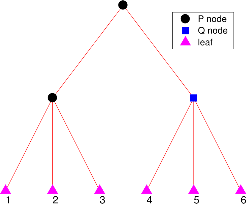
A PQ-tree represents permutations of the elements of a set through admissible reorderings of its leaves. Each transformation in Definition 2 specifies an admissible reordering of the nodes within a PQ-tree. For example, a tree with a single P-node represents the equivalence class of all permutations of the elements of $U$, while a tree with a single Q-node represents both the left-to-right and right-to-left orderings of the leaves. A tree with a mixed P-node and Q-node structure represents the equivalence class of a constrained permutation, where the exact structure of the tree determines the constraints. Figure 1 displays a PQ-tree and the admissible permutations it represents.

1	2	3	4	5	6
1	2	3	6	5	4
1	3	2	4	5	6
1	3	2	6	5	4
2	1	3	4	5	6
2	1	3	6	5	4
2	3	1	4	5	6
2	3	1	6	5	4
3	1	2	4	5	6
3	1	2	6	5	4
3	2	1	4	5	6
3	2	1	6	5	4
4	5	6	1	2	3
4	5	6	1	3	2
4	5	6	2	1	3
4	5	6	2	3	1
4	5	6	3	1	2
4	5	6	3	2	1
6	5	4	1	2	3
6	5	4	1	3	2
6	5	4	2	1	3
6	5	4	2	3	1
6	5	4	3	1	2
6	5	4	3	2	1

Fig. 1: On the left, a PQ-tree over the set $U=\{1,\ldots,6\}$; on the right, the 24 admissible permutations encoded in the tree.

The PQ-tree data structure has been exploited in a variety of applications, from archaeology and chronology reconstruction [1] to molecular biology with DNA mapping and sequence assembly [22]. The first problem to which it was applied is the consecutive ones property (C1P) for matrices [4], mentioned in Section 1.

Given a pre-R matrix, the spectral algorithm from [1], that will be discussed in Section 4, constructs a PQ-tree describing the set of all the permutations of rows and columns that lead to an R-matrix.

3.1 Implementation of PQ-trees

The PQser toolbox for Matlab is available as a compressed archive that can be downloaded from the authors webpages (see, e.g., http://bugs.unica.it/~gppe/soft/). By uncompressing it, the directory PQser will be created. It must be added to Matlab search path, either by the command addpath or using the graphical interface menus. The sub-directory demo contains a tutorial for the toolbox and the scripts which were used to construct the examples reported in the paper. The installation procedure and the toolbox content are described in detail in the README.txt file, which can be found in the main directory.

In the PQser toolbox, a PQ-tree $T$ is a struct variable (i.e., a record) composed by two fields. The first field, T.type, specifies the type of the node, i.e., P, Q, or a leaf, in the case of a trivial tree. The second field, T.value, is a vector which provides a list of PQ-trees, recursively defined. In the case of a leaf, this field contains the index of the unit it represents.

For example, the graph in Figure 1 was obtained by the following piece of code

v(1) = pnode([1 2 3]);Ψ% create a P-node with three leaves
v(2) = qnode([4 5 6]);Ψ% create a Q-node with three leaves
T = pnode(v);ΨΨ% create a P node pointing to the previous two nodes
pqtreeplot(T)ΨΨ% visualize the PQ-tree

the resulting data structure for the PQ-tree is

T =
  struct with fields:
     type: ’P’
    value: [1x2 struct]

and the permutations encoded in $T$ are computed by

perms_matrix = pqtreeperms(T)

These instructions are contained in the script graf1.m, in the demo sub-directory.

pnode	create a P-node
qnode	create a Q-node
lnode	create a leaf
mnode	create an M-node
pqtreeplot	plot a PQ-tree
pqtreeNperm	number of admissible permutations in a PQ-tree
pqtreeperms	extract all admissible permutations from a PQ-tree
pqtree1perm	extract one admissible permutation from a PQ-tree
pqtreegetnode	extract a subtree from a PQ-tree
pqtreenodes	converts a PQ-tree to Matlab treeplot format

Table 2: Functions in the PQser toolbox devoted to the manipulation of PQ-trees.

The functions intended for creating and manipulating a PQ-tree are listed in Table 2. The function mnode creates an additional type of node, an M-node, which is intended to deal with multiple Fiedler values; we will comment on it in Section 5; pqtreegetnode and pqtreenodes are utility functions for pqtreeplot, they are not intended to be called directly by the user. All the functions are documented via the usual Matlab help command, e.g.,

help pnode
help pqtreeplot

As an example, we report in Algorithm 1 the structure of pqtreeNperm, a function which returns the number $N$ of all the permutations contained in the tree whose root $T$ is given in input. In the particular case of a leaf, only one permutation is possible (line 2–3). Otherwise, we consider the vector $\mathbf{c}$ of size $k$, containing the children nodes of the root of T (line 5). The algorithm calls itself recursively on each component of $\mathbf{c}$ (line 8). In the case of a Q-node the number of permutations is doubled, because only one ordering and its reverse are admissible, whereas for a P-node the number is multiplied by the factorial of $k$, since in this case all the possible permutations of the children are allowed. The same procedure is applied to an M-node; see Section 5 for details.

• function $N=\operatorname{\textsf{pqtreeNperm}}(T)$

• if $T$ is a leaf

• $N=1$

• else

• $\mathbf{c}=T\texttt{.value}$, $k=\operatorname{length}(\mathbf{c})$

• $p=1$

• for $i=1,\dots,k$

• $p=p*\operatorname{\textsf{pqtreeNperm}}(c_{i})$

• end for

• if $T$ is a Q-node

• $N=2*p$

• else

• $N=\operatorname{factorial}(k)*p$

• end if

• end if

Algorithm 1 Compute the number of admissible permutations in a PQ-tree.

The toolbox includes an interactive graphical tool for exploring a PQ-tree $T$. After displaying $T$ by pqtreeplot, it is possible to extract a subtree by clicking on one node with the left mouse button. In this case, the corresponding subtree is extracted, it is plotted in a new figure, and it is saved to the variable PQsubtree in the workspace. This feature is particularly useful when analyzing a large PQ-tree. The function pqtreeplot allows to set some attributes of the plot; see the help page.

4 A spectral algorithm for the seriation problem

In this section we briefly review the spectral algorithm for the seriation problem introduced in [1], and describe our implementation.

Given the set of units $U=\{u_{1},u_{2},\dots,u_{n}\}$, we will write $i\preccurlyeq j$ if $u_{i}$ precedes $u_{j}$ in a chosen ordering. In [1], the authors consider a symmetric bivariate correlation function $f$ reflecting the desire for units $i$ and $j$ to be close to each other in the sought sequence. The point is to find all index permutation vectors ${\boldsymbol{\pi}}=(\pi_{1},\ldots,\pi_{n})^{T}$ such that

$$\pi_{i}\preccurlyeq\pi_{j}\preccurlyeq\pi_{k}\quad\iff\quad f(\pi_{i},\pi_{j})\geq f(\pi_{i},\pi_{k})\quad\text{and}\quad f(\pi_{j},\pi_{k})\geq f(\pi_{i},\pi_{k}).$$ (4.1)

It is natural to associate to such correlation function a real symmetric matrix $F$, whose entries are defined by $f_{ij}=f(i,j)$. This matrix plays exactly the role of the similarity matrix $S$ discussed in Section 2, as the following theorem states.

Theorem 3.

A matrix $F$ is an R-matrix if and only if (4.1) holds.

Proof.

Let us assume that the permutation ${\boldsymbol{\pi}}$ which realizes (4.1) has already been applied to the units. Then, since a permutation of the units corresponds to a simultaneous permutation of the rows and columns of the matrix $F$, we obtain

$$i\leq j\leq k\quad\iff\quad f_{ij}\geq f_{ik}\quad\text{and}\quad f_{jk}\geq f_{ik}.$$

The first inequality $f_{ij}\geq f_{ik}$ is exactly (2.2). Keeping into account the symmetry of $F$ and cyclically permuting the indexes, from the second inequality we get

$$j\leq k\leq i\quad\iff\quad f_{ij}\leq f_{ik},$$

which corresponds to (2.1). ∎

If a seriation data set is described by an adjacency (or abundance) matrix $A$, we will set $F=AA^{T}$. If $F$ is pre-$R$ (see Section 2), there exists a rows/columns permutation that takes it in $R$-form. Unfortunately, this property cannot be stated in advance, in general. This property can be ascertained, e.g., after applying the algorithm discussed in this section; see below.

The authors approach in [1], see also [14], is to consider the minimization of the following penalty function

$$h(\mathbf{x})=\frac{1}{2}\sum_{i,j=1}^{n}f_{ij}(x_{i}-x_{j})^{2},\quad\mathbf{x}\in{\mathbb{R}}^{n},$$

whose value is small for a vector $\mathbf{x}$ such that each pair $(i,j)$ of highly correlated units is associated to components $x_{i}$ and $x_{j}$ with close values. Once the minimizing vector $\mathbf{x}_{\min}$ is computed, it is sorted in either nonincreasing or nondecreasing value order, yielding $\mathbf{x}_{\boldsymbol{\pi}}=(x_{\pi_{1}},\ldots,x_{\pi_{n}})^{T}$. The permutation of the units ${\boldsymbol{\pi}}$ realizes (4.1).

Note that $h$ does not have a unique minimizer, since its value does not change if a constant is added to each of the components $x_{i}$ of the vector $\mathbf{x}$. In order to ensure uniqueness and to rule out the trivial solution, it is necessary to impose two suitable constraints on the components of the vector $\mathbf{x}$. The resulting minimization problem is:

minimize $$h(\mathbf{x})=\frac{1}{2}\sum_{i,j=1}^{n}f_{ij}(x_{i}-x_{j})^{2}$$

subject to $$\sum_{i}x_{i}=0\quad\text{and}\quad\sum_{i}x_{i}^{2}=1.$$

The solution to this approximated problem may be obtained from the Fiedler vector of the Laplacian $L$ of the correlation matrix $F$. Letting $D=\mathop{\operator@font diag}\nolimits(d_{i})$ be the degree matrix, $d_{i}=\sum_{j=1}^{n}f_{ij}$, it is immediate to observe that

$$h(\mathbf{x})=\frac{1}{2}\sum_{i,j=1}^{n}f_{ij}(x_{i}^{2}+x_{j}^{2}-2x_{i}x_{j})=\mathbf{x}^{T}D\mathbf{x}-\mathbf{x}^{T}F\mathbf{x}.$$

This shows that the previous minimization problem can be rewritten as

$$\min_{\|\mathbf{x}\|=1,\ \mathbf{x}^{T}\mathbf{e}=0}\mathbf{x}^{T}L\mathbf{x}$$

where $L=D-F$. The constraints require $\mathbf{x}$ to be a unit vector orthogonal to $\mathbf{e}$. Being $L$ symmetric, all the eigenvectors except $\mathbf{e}$ satisfy the constraints. Consequently, a Fiedler vector is a solution to the constrained minimization problem.

In fact, Theorem 3.2 from [1] proves that an R-matrix has a monotone Fiedler vector, while Theorem 3.3, under suitable assumptions, implies that a reordering of the Fiedler vector takes a pre-R matrix to R-form. This confirms that the problem is well posed only when $F$ is pre-R. Nevertheless, real data sets may be inconsistent, in the sense that do not necessarily lead to pre-R similarity matrices. In such cases, it may be useful to construct an approximate solution to the seriation problem, and sorting the entries of the Fiedler vector generates an ordering that tries to keep highly correlated elements close to each other. This is relevant because techniques based on Fiedler vectors are being used for the solution of different sequencing problems [3, 22, 24, 26]. In particular, they are employed in complex network analysis, e.g., for community detection and partitioning of graphs [13, 15].

The algorithm proposed in [1] is based upon the above idea, and uses a PQ-tree to store the permutations of the units that produce a solution to the seriation problem; its implementation is described in Algorithm 2.

• function $T=\operatorname{\textsf{spectrsort}}(F,U)$

• $n=$ row size of $F$

• $\alpha=\min_{i,j}f_{i,j}$, if $\alpha\neq 0$, $\mathbf{e}=(1,\ldots,1)^{T}$, $F=F-\alpha\mathbf{e}\mathbf{e}^{T}$, end

• call $\operatorname{\textsf{getconcomp}}$ to construct the connected components $\{F_{1},\dots,F_{k}\}$ of $F$

• XXX and the corresponding index sets $U=\{U_{1},\dots,U_{k}\}$

• if $k>1$

• for $j=1,\dots,k$

• $v(j)=\operatorname{\textsf{spectrsort}}(F_{j},U_{j})$

• end for

• $T=\operatorname{\textsf{pnode}}(v)$

• else

• if $n=1$

• $T=\operatorname{\textsf{lnode}}(U)$

• else if $n=2$

• $T=\operatorname{\textsf{pnode}}(U)$

• else

• $L=$ Laplacian matrix of $F$

• compute (part of) the eigenvalues and eigenvectors of $L$

• determine multiplicity $n_{F}$ of the Fiedler value according to a tolerance $\tau$

• if $n_{F}=1$

• $\mathbf{x}=$ sorted Fiedler vector

• $t$ number of distinct values in $\mathbf{x}$ according to a tolerance $\tau$

• for $j=1,\dots,t$

• $u_{j}$ indices of elements in $\mathbf{x}$ with value $x_{j}$

• if $u_{j}$ has just one element

• $v_{j}=\operatorname{\textsf{lnode}}(u_{j})$

• else

• $v(j)=\operatorname{\textsf{spectrsort}}(F(u_{j},u_{j}),U(u_{j},u_{j}))$

• end if

• end for

• $T=\operatorname{\textsf{qnode}}(v)$

• else

• $T=\operatorname{\textsf{mnode}}(U)$

• end if

• end if

• end if

Algorithm 2 Spectral sort algorithm.

The algorithm starts translating all the entries of the correlation matrix so that the smallest is 0 , i.e.,

$$\tilde{F}=F-\alpha\mathbf{e}\mathbf{e}^{T},\qquad\alpha=\min_{i,j}f_{ij};$$ (4.2)

see line 3 of Algorithm 2. This is justified by the fact that $F$ and $\tilde{F}$ have the same Fiedler vectors and that if $F$ is an irreducible R-matrix such translation ensures that the Fiedler value is a simple eigenvalue of $L$ [1, Lemma 4.1 and Theorem 4.6]. Our software allows the user to disable this procedure (see Table 4 below) as he may decide to suitably preprocess the similarity matrix in order to reduce the computational load. Indeed, the translation procedure is repeated each time the algorithm calls itself recursively.

• function $U=\operatorname{\textsf{getconcomp}}(F)$

• preallocate the cell-array $U$, $chlist=$empty vector

• $root=${node 1}, $list=root$, $n=$row size of $F$

• $i=0$, $flag=true$ (logical variable)

• while $flag$

• $i=i+1$

• $list=\operatorname{\textsf{graphvisit}}(root,list)$

• $U\{i\}=list$

• update $chlist$ adding the nodes in $list$ and sort the vector

• $flag=true$ if the number of elements in $chlist$ is different from $n$

• XXX otherwise $flag=false$

• if $flag$

• choose the $root$ for a new connected component

• if there are no connected components left

• exit

• end if

• $list=root$

• end if

• end while

Algorithm 3 Detect the connected components of a graph.

If the matrix $F$ is reducible, then the seriation problem can be decoupled [1, Lemma 4.2]. Lines 4–5 of the algorithm detect the irreducible blocks of the correlation matrix by using the function getconcomp.m, which also identifies the corresponding index sets. The function, described in Algorithm 3, constructs a cell array containing the indices which identify each connected component of a graph. It calls the function graphvisit.m, which visits a graph starting from a chosen node; see Algorithm 4. Note that these two functions, in order to reduce the stack consumption due to recursion, use a global variable to store the correlation matrix.

• function $list=\operatorname{\textsf{graphvisit}}(root,list)$

• construct the list $l$ of the indices of the nodes connected to the root

• initialize an empty list $nlist$

• find the elements of $l$ which are not in $list$

• add the new elements to $list$ and to $nlist$

• if $nlist$ is not empty

• sort $list$

• for each node $i$ in $nlist$

• $list=\operatorname{\textsf{graphvisit}}(nlist(i),list)$

• end for

• end if

Algorithm 4 Visit a graph starting from a node.

If more than one connected component is found, then the function calls itself on each component, and stores the returned lists of nodes as children of a P-node (lines 7–10). If the matrix is irreducible, the dimension $n$ of the matrix is considered (lines 12–16). The cases $n=1,2$ are trivial. If $n>2$, the Laplacian matrix $L$ is computed, as well as the Fiedler value and vector (lines 17–18). Depending on the matrix being “small” or “large” different algorithms are used. For a small scale problem the full spectral decomposition of the Laplacian is computed by the eig function of Matlab. For a large scale problem only a small subset of the eigenvalues and eigenvectors are evaluated using the eigs function, which is based on a Krylov space projection method. The PQser toolbox computes by default the eigenpairs corresponding to the three eigenvalues of smallest magnitude, since they are sufficient to understand if the Fiedler value is simple or multiple, but the default value can be modified. The choice between the two approaches is automatically performed and it may be influenced by the user; see Table 4 in Section 4.1.

Then, the algorithm determines the multiplicity of the Fiedler value according to a given tolerance. If the Fiedler value is a simple eigenvalue of $L$, the algorithm sorts the elements of the current list according to the reordering of the Fiedler vector and stores them as the children of a Q-node. If two or more values of the Fiedler vector are repeated the function invokes itself recursively (line 28), in accordance with [1, Theorem 4.7]; on the contrary, the corresponding node becomes a leaf (line 26). In our implementation we introduce a tolerance $\tau$ to distinguish “equal” and “different” numbers: $a$ and $b$ are considered “equal” if $|a-b|<\tau$. The default value for $\tau$ is $10^{-8}$.

In the case of a multiple Fiedler value, the algorithm conventionally constructs an “M-node” (line 33). This new type of node has been introduced in order to flag this particular situation, which will be further discussed in Section 5.

Algorithm 2 produces a PQ-tree whether $F$ is a pre-R matrix or not. If all the Fiedler values computed are simple, the starting matrix is pre-R and any permutation encoded in the PQ-tree will take it to R-form. In the presence of a multiple Fiedler vector the problem is not well posed and an approximate solution is computed.

The number $N$ of all the admissible permutations generated by the algorithm can be obtained by counting all the admissible boundaries of the tree. In the case of a PQ-tree consisting of a single Q-node $N$ is equal to 2, because only the left-to-right order of the children leaves and its reverse are possible. For a single P-node, the number of all the permutations is the factorial of the number of the children. An M-node is temporarily treated as a P-node, although we experimentally observed that not all the permutations are admissible; this aspect is discussed in Section 5.

4.1 Implementation of spectral seriation

The functions included in the PQser toolbox are listed in Table 3. Besides the function spectrsort, which implements Algorithm 2, there is a parallel version of the same method, pspectrsort, which distributes the for loop at line 7 of the algorithm among the available processing units. In order to execute the function pspectrsort, the Parallel Computing Toolbox must be present in the current Matlab installation.

spectrsort	spectral sort for the seriation problem
pspectrsort	parallel version of spectrsort
fiedvecs	compute the Fiedler vectors and values of a Laplacian
getconcomp	determine the connected components of a graph
graphvisit	visit a graph starting from a node
distinct	sort and level the elements of a vector
lapl	construct the graph Laplacian of a matrix
testmatr	test matrices for PQser

Table 3: Functions in the PQser toolbox devoted to the solution of the seriation problem.

The function testmatr allows one to create some simple test problems. The remaining functions of Table 3 are not likely to be used in the common use of the toolbox. They are made available to the expert user, who may decide to call them directly or to modify their content.

tau	tolerance used to distinguish between “equal” and “different”
	values (spectrsort and fiedvecs, def. $10^{-8}$)
translate	applies translation (4.2) (spectrsort, def. 1)
lrg	used to select small scale or large scale algorithm (fiedvecs,
	true if the input matrix is sparse)
nlarge	if matrix size is below this value, the small scale algorithm
	is used (fiedvecs, def. 1000)
neig	number of eigenpairs to be computed when the large scale
	algorithm is used (fiedvecs, def. 3)
maxncomp	maximum number of connected components (getconcomp, def. 100)
bw	half bandwidth of test matrix (testmatr, type 2 example, def. 2)
spar	construct a sparse test matrix (testmatr, type 2 example, def. 1)

Table 4: Tuning parameters for the PQser toolbox; the functions affected are reported in parentheses, together with the default value of each parameter.

The toolbox has some tuning parameters, which are set to a default value, but can be modified by the user. This can be done by passing to a function, as an optional argument, a variable of type struct with fields chosen among the ones listed in Table 4. For example:

opts.translate = 0;
T = spectrsort(F,opts);

applies Algorithm 2 to a similarity matrix $F$ omitting the translation process described in (4.2).

To illustrate the use of the toolbox, we consider a similarity matrix $R$ satisfying the Robinson criterion

$$R=\begin{bmatrix}200&150&120&80&40&0&0&0&0&0\\ 150&200&160&120&80&40&0&0&0&0\\ 120&160&200&160&120&80&40&0&0&0\\ 80&120&160&200&160&120&80&40&0&0\\ 40&80&120&160&200&160&120&80&40&0\\ 0&40&80&120&160&200&160&120&80&40\\ 0&0&40&80&120&160&200&160&120&80\\ 0&0&0&40&80&120&160&200&160&120\\ 0&0&0&0&40&80&120&160&200&150\\ 0&0&0&0&0&40&80&120&150&200\end{bmatrix}$$

and the pre-R matrix obtained by applying to the rows and columns of $R$ a random permutation

$$F=\begin{bmatrix}200&0&0&150&120&0&160&40&0&80\\ 0&200&150&0&0&120&0&80&160&40\\ 0&150&200&0&0&80&0&40&120&0\\ 150&0&0&200&80&0&120&0&0&40\\ 120&0&0&80&200&80&160&120&40&160\\ 0&120&80&0&80&200&40&160&160&120\\ 160&0&0&120&160&40&200&80&0&120\\ 40&80&40&0&120&160&80&200&120&160\\ 0&160&120&0&40&160&0&120&200&80\\ 80&40&0&40&160&120&120&160&80&200\end{bmatrix}.$$

The PQ-tree $T$ containing the solution of the reordering problem is constructed by calling the function spectrsort, which returns the resulting data structure:

T = spectrsort(F,opts)
T =
  struct with fields:
     type: ’Q’
    value: [1x10 struct]

Using the function pqtreeplot

pqtreeplot(T)

we obtain the representation of the PQ-tree displayed in Figure 2.

Fig. 2: A PQ-tree corresponding to a pre-R matrix of dimension 10.

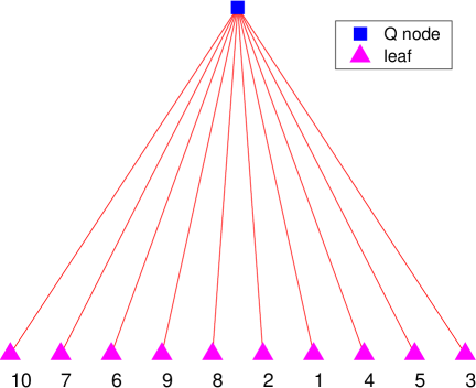
In this particular case, the PQ-tree $T$ consists of just a Q-node as a root, so only two permutations of the leaves are allowed. They can be extracted from the tree using the function pqtreeperms, whose output is

perms_matrix = pqtreeperms(T)
perms_matrix =
     4     1     7     5    10     8     6     9     2     3
     3     2     9     6     8    10     5     7     1     4

In some occasions, a PQ-tree may contain a very large number of permutations. In such cases, the function pqtree1perm extracts just one of the permutations, in order to apply it to the rows and columns of the matrix $F$:

seq = pqtree1perm(T);
AR = F(seq,seq);

Since $F$ is pre-R, we clearly reconstruct the starting similarity matrix $R$.

This experiment is contained in the script graf2.m, in the demo sub-directory. The script tutorial.m, in the same directory, illustrates the use of the toolbox on other numerical examples.

5 The case of a multiple Fiedler value

In this section we discuss the case where the Fiedler value is a multiple root of the characteristic polynomial of the Laplacian $L$. When this happens, the eigenspace corresponding to the smallest nonzero eigenvalue of $L$ has dimension larger than one, so there is no uniqueness in the choice of the Fiedler vector.

We conjecture that sorting the entries of a Fiedler vector, that is, of any vector in the eigenspace of the Fiedler value, does not necessarily lead to all possible indexes permutations, i.e., the factorial of the number $n$ of units. We observed that there may be some constraints that limit the number of permutations deriving from the Fiedler vector, and this number does not appear to be related to the multiplicity of the Fiedler value by a simple formula. We will illustrate this issue by a numerical experiment.

As we did not find any reference to this problem in the literature, we plan to study it in a subsequent paper. This is the reason why the PQser toolbox conventionally associates an M-node, to the presence of a multiple Fiedler value. In the software, the new type of node is temporarily treated as a P-node. This leaves the possibility to implement the correct treatment of the case, once the problem will be understood.

Fig. 3: The cycle seriation problem; the units are on the left, the types on the right.

Here we present a simple example to justify our conjecture. Let us consider the seriation problem described by the bipartite graph depicted in Figure 3. The nodes on the left are the units, e.g., the excavation sites; on the right there are the types, which may be seen as the archeological findings. The relationships between units and types are represented by edges connecting the nodes.

The problem is clearly unsolvable, as the associated graph describes a cycle: each unit is related to surrounding units by a connection to a common type, and the two extremal units are related to each other in the same way.

At the same time, not all the units permutations are admissible. For example, one may argue that the permutation ${\boldsymbol{\pi}}_{1}=(3,4,5,1,2)^{T}$ should be considered partially feasible, as it breaks only one of the constraints contained in the bipartite graph, while the ordering ${\boldsymbol{\pi}}_{2}=(1,4,2,5,3)^{T}$ has nothing to do with the problem considered.

The adjacency matrix associated to the graph in Figure 3 is the following

$$A=\begin{bmatrix}1&1&0&0&0\\ 0&1&1&0&0\\ 0&0&1&1&0\\ 0&0&0&1&1\\ 1&0&0&0&1\end{bmatrix}.$$ (5.1)

We can associate to (5.1) the similarity matrix

$$F=AA^{T}=\begin{bmatrix}2&1&0&0&1\\ 1&2&1&0&0\\ 0&1&2&1&0\\ 0&0&1&2&1\\ 1&0&0&1&2\end{bmatrix},$$ (5.2)

whose Laplacian is

$$L=D-F=\begin{bmatrix}2&-1&0&0&-1\\ -1&2&-1&0&0\\ 0&-1&2&-1&0\\ 0&0&-1&2&-1\\ -1&0&0&-1&2\end{bmatrix}.$$

The matrix $L$ is circulant, that is, it is fully specified by its first column, while the other columns are cyclic permutations of the first one with an offset equal to the column index. A complete treatment of circulant matrices can be found in [10], while [39] implements a Matlab class for optimized circulant matrix computations.

One of the basic properties of circulant matrices is that their spectrum is analytically known. In particular, the eigenvalues of $L$ are given by

$$\{\widehat{L}(1),\widehat{L}(\omega),\widehat{L}(\omega^{2}),\widehat{L}(\omega^{3}),\widehat{L}(\omega^{4})\},$$

where $\widehat{L}(\zeta)$ is the discrete Fourier transform of the first column of $L$

$$\hat{L}(\zeta)=2-\zeta^{-1}-\zeta^{-4},$$

and $\omega={\mathrm{e}}^{\frac{2\pi{\mathrm{i}}}{5}}$ is the minimal phase $5$th root of unity; see [10]. A simple computation shows that

$$\widehat{L}(1)=0,\quad\widehat{L}(\omega)=\widehat{L}(\omega^{4})=2-2\cos\frac{2\pi}{5},\quad\widehat{L}(\omega^{2})=\widehat{L}(\omega^{3})=2-2\cos\frac{4\pi}{5},$$

so that the Fiedler value $\widehat{L}(\omega)$ has multiplicity 2.

To explore this situation we performed the following numerical experiment. We considered 10000 random linear combinations of an orthonormal basis for the eigenspace corresponding to the Fiedler value. This produces a set of random vectors, belonging to a plane immersed in ${\mathbb{R}}^{5}$, which can all be considered as legitimate “Fiedler vectors”.

Each vector was sorted, and the corresponding permutations of indexes were stored in the columns of a matrix. In the end, all the repeated permutations were removed. We obtained 10 permutations, reported in the columns of the following matrix

$$\begin{bmatrix}3&2&5&3&2&4&4&1&5&1\\ 2&1&4&4&3&3&5&5&1&2\\ 4&3&1&2&1&5&3&2&4&5\\ 1&5&3&5&4&2&1&4&2&3\\ 5&4&2&1&5&1&2&3&3&4\end{bmatrix}.$$ (5.3)

They are much less than the $5!=120$ possible permutations, and reduce to 5 if we remove the columns which are the reverse of another column. This confirms our conjecture: when a Fiedler value is multiple some constraints are imposed on the admissible permutations of the units.

It is relevant to notice that matrix (5.3) does not contain the cyclic permutations of the units depicted in Figure 3. Indeed, the spectral algorithm aims at moving the nonzero components close to the main diagonal, and this contrasts with the presence of nonzeros in the elements $f_{51}$ and $f_{15}$ of matrix (5.2). All permutations contained in (5.3), when applied to the similarity matrix $F$, produce the same matrix

$$\tilde{F}=\begin{bmatrix}2&1&1&0&0\\ 1&2&0&1&0\\ 1&0&2&0&1\\ 0&1&0&2&1\\ 0&0&1&1&2\end{bmatrix},$$

which exhibits a smaller bandwidth than (5.2).

This experiment can be reproduced by executing the script mfiedval.m, which is found in the demo sub-directory.

6 Numerical experiments

In this section we illustrate the application of the PQser toolbox to some numerical examples. The experiments can be repeated by running the related Matlab scripts located in the demo sub-directory of the toolbox.

Fig. 4: Processing of the Bornholm data set: the spy plot on the left shows the original matrix, a permuted version is reported in the central graph, on the right we display the matrix reordered by the spectral algorithm.

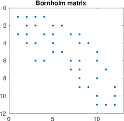
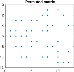
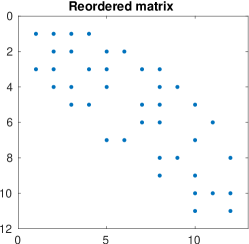
The first example is the numerical processing of the Bornholm data set, presented in Table 1. We randomly permute the rows of the adjacency matrix and apply the spectral algorithm to the similarity matrix associated to the permuted matrix. The resulting PQ-tree contains just a Q-node, so there is only one solution (actually, this is a proof that the matrix is pre-R) which we use to reorder the permuted matrix. The computational code is contained in the file exper1.m.

Figure 4 reports the spy plots which represent the nonzero entries of the initial matrix, its permuted version, and the final reordering. It is immediate to observe that the lower band of the reordered matrix is slightly narrower than the initial matrix, showing that the spectral algorithm was able to improve the results obtained empirically by archaeologists.

The second example concerns the comparison of the spectral algorithm with its parallel version in the solution of a large scale problem. The experiments were performed on a dual Xeon CPU E5-2620 system (12 cores), running the Debian GNU/Linux operating system and Matlab 9.2.

The function testmatr of the toolbox allows the user to create a block diagonal matrix, formed by $m$ banded blocks whose size is chosen using a second input parameter. The matrix is randomly permuted in order to hide its reducible structure.

Fig. 5: Comparison between the sequential and the parallel versions of Algorithm 2: on the left the execution time in seconds, on the right the parallel speedup, defined as the ratio between the sequential and the parallel timings. The test matrix is of dimension $2^{15}=32768$, the size of each reducible block is $2^{j}$, where $j$ is the index reported in the horizontal axis.

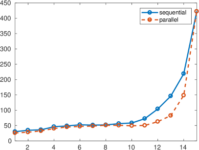
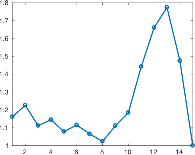
We let the size of the problem be $n=2^{15}=32768$ and, for $j=1,2\ldots,15$, we generate a sequence of test matrices containing $n\cdot 2^{-j}$ blocks, each of size $2^{j}$.

We apply the function spectrsort that implements Algorithm 2 to the above problems, as well as its parallel version pspectrsort, and record the execution time; see the file exper2.m. The number of processors available on our computer was 12.

The graph on the left of Figure 5 shows that there is a significant advantage from running the toolbox on a parallel computing system when the network associated to the problem is composed by a small number of large connected components. This is confirmed by the plot of the parallel speedup, that is, the ratio between the timings of the sequential and the parallel implementations, displayed in the graph on the right in the same figure.

Fig. 6: Bandwidth reduction of a sparse matrix of size 1024: the three spy plots display the initial matrix, the reordered matrix resulting from the spectral algorithm, and the one produced by the symrcm function of Matlab.

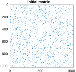
To conclude, we consider another important application of the reordering defined by the Fiedler vector of the Laplacian, namely, the reduction of the bandwidth for a sparse matrix; see [3].

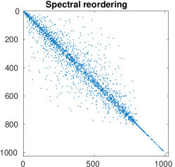
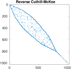
We generate a sparse symmetric matrix of size $n=1024$, having approximately 0.2% nonzero elements, and reorder its rows and columns by Algorithm 2. Notice that in this case the spectral algorithm must be applied to a matrix whose elements are taken in absolute value. The computation is described in the script exper3.m.

The resulting matrix is depicted by displaying its nonzero pattern in Figure 6, where it is compared to the reverse Cuthill-McKee ordering, as implemented in the symrcm function of Matlab. The spectral algorithm appears to be less effective than symrcm, leading to a reordered matrix with a wider band. This is due to the fact that spectrsort aims at placing the largest entries close to the diagonal, and this does not necessarily produce the maximal bandwidth reduction. Experimenting with sparser matrices we observed that often the two methods produce similar results.

We remark that, also in this application, the presence of a multiple Fiedler value may constitute a problem. For example, we were not able to correctly process the Matlab test matrix bucky (the connectivity graph of the Buckminster Fuller geodesic dome), because the associated Laplacian possesses a triple Fiedler value.

7 Conclusions

In this paper we present a new Matlab toolbox principally aimed to the solution of the seriation problem, but which can be applied to other related problems.

It is based on a spectral algorithm introduced in [1], and contains an implementation of PQ-trees as well as some tools for their manipulation, including an interactive visualization tool. The implemented algorithm includes the possibility to choose between a small scale and a large scale algorithm for the computation of the Fiedler vector, and to detect equal components in the same vector according to a chosen tolerance. Further, a parallel version of the method is provided.

We also point out the importance of the presence of multiple Fiedler values, a problem which has not been considered before in the literature and which has a significant influence on the computation of an approximate solution to the seriation problem.

The use of the toolbox is illustrated by a few practical examples, and its performance is investigated through a set of numerical experiments, both of small and large scale.

8 Acknowledgements

We would like to thank Matteo Sommacal for pointing our attention to the problem of seriation and to its application in archaeology. The paper [37], which he coauthored, was our principal source of information when the research which lead to this paper started.

References

- [1] J. E. Atkins, E. G. Boman, and B. Hendrickson. A spectral algorithm for seriation and the consecutive ones problem. SIAM J. Comput., 28(1):297–310, 1998.
- [2] J. A. Barcelo and I. Bogdanovic. Mathematics and Archaeology. CRC Press, 2015.
- [3] S. T. Barnard, A. Pothen, and H. Simon. A spectral algorithm for envelope reduction of sparse matrices. Numer. Linear Algebra Appl., 2(4):317–334, 1995.
- [4] K. S. Booth and G. S. Lueker. Testing for the consecutive ones property, interval graphs, and graph planarity using PQ-tree algorithms. J. Comput. Syst. Sci., 13(3):335–379, 1976.
- [5] G. W. Brainerd. The place of chronological ordering in archaeological analysis. Am. Antiq., 16(4):301–313, 1951.
- [6] M. J. Brusco and D. Steinley. Clustering, seriation, and subset extraction of confusion data. Psychol. Methods, 11(3):271–286, 2006.
- [7] G. Caraux and S. Pinloche. PermutMatrix: a graphical environment to arrange gene expression profiles in optimal linear order. Bioinformatics, 21(7):1280–1281, 1979. Package available at http://www.atgc-montpellier.fr/permutmatrix/.
- [8] V. Chepoi and B. Fichet. Recognition of Robinsonian dissimilarities. J. Classif., 14(2):311–325, 1997.
- [9] T. Christof, M. Oswald, and G. Reinelt. Consecutive ones and a betweenness problem in computational biology. In International Conference on Integer Programming and Combinatorial Optimization, pages 213–228. Springer, 1998.
- [10] P. J. Davis. Circulant Matrices. Wiley, New York, 1979.
- [11] N. M. M. De Abreu. Old and new results on algebraic connectivity of graphs. Linear Algebra Appl., 423(1):53–73, 2007.
- [12] M. B. Eisen, P. T. Spellman, P. O. Brown, and D. Botstein. Cluster analysis and display of genome-wide expression patterns. P. Natl. Acad. Sci. U.S.A., 95:14863–14868, 1998.
- [13] E. Estrada. The Structure of Complex Networks: Theory and Applications. Oxford University Press, 2012.
- [14] E. Estrada and D. J. Higham. Network properties revealed through matrix functions. SIAM Rev., 52(4):696–714, 2010.
- [15] E. Estrada and P. Knight. A First Course in Network Theory. Oxford University Press, 2015.
- [16] M. Fiedler. Algebraic connectivity of graphs. Czech. Math. J., 23(2):298–305, 1973.
- [17] M. Fiedler. A property of eigenvectors of nonnegative symmetric matrices and its application to graph theory. Czech. Math. J., 25(4):619–633, 1975.
- [18] M. Fiedler. Laplacian of graphs and algebraic connectivity. Banach Center Publ., 25(1):57–70, 1989.
- [19] F. Fogel, A. d’Aspremont, and M. Vojnovic. Serialrank: Spectral ranking using seriation. In Advances in Neural Information Processing Systems 27, pages 900–908, 2014.
- [20] F. Fogel, R. Jenatton, F. Bach, and A. d’Aspremont. Convex relaxations for permutation problems. SIAM J. Matrix Anal. Appl., 36(4):1465–1488, 2015.
- [21] D. Fulkerson and O. Gross. Incidence matrices and interval graphs. Pac. J. Math., 15(3):835–855, 1965.
- [22] D. S. Greenberg and S. Istrail. Physical mapping by STS hybridization: Algorithmic strategies and the challenge of software evaluation. J. Comput. Biol., 2(2):219–273, 1995.
- [23] M. Hahsler, K. Hornik, and C. Buchta. Getting things in order: an introduction to the R package seriation. J. Stat. Softw., 25(3):1–34, 2008.
- [24] D. J. Higham, G. Kalna, and M. Kibble. Spectral clustering and its use in bioinformatics. J. Comput. Appl. Math., 204(1):25–37, 2007.
- [25] F. R. Hodson, D. G. Kendall, and P. Tautu. Mathematics in the Archaeological and Historical Sciences. Edimburg University Press, Edimburg, 1971.
- [26] M. Juvan and B. Mohar. Optimal linear labelings and eigenvalues of graphs. Discrete Appl. Math., 36(2):153–168, 1992.
- [27] D. G. Kendall. A statistical approach to Flinders–Petries sequence-dating. Bull. Int. Stat. Inst., 40(2):657–681, 1963.
- [28] D. G. Kendall. Incidence matrices, interval graphs and seriation in archeology. Pac. J. Math., 28(3):565–570, 1969.
- [29] D. G. Kendall. A mathematical approach to seriation. Philos. Trans. R. Soc. A-Math. Phys. Eng. Sci., 269(1193):125–134, 1970.
- [30] M. Laurent and M. Seminaroti. A Lex-BFS-based recognition algorithm for Robinsonian matrices. Discret. Appl. Math., 222:151–165, 2017.
- [31] M. Laurent and M. Seminaroti. Similarity-First Search: a new algorithm with application to Robinsonian matrix recognition. SIAM Discret. Math., 31(3):1765–1800, 2017.
- [32] I. Liiv. Seriation and matrix reordering methods: an historical overview. Stat. Anal. Data Min., 3(2):70–91, 2010.
- [33] B. G. Mirkin and S. N. Rodin. Graphs and Genes, volume 11 of Biomathematics. Springer-Verlag, 1984.
- [34] M. J. O’Brien and R. L. Lyman. Seriation Stratigraphy and Index Fossils: The Backbone of Archaeological Dating. Kluwer, 2002.
- [35] M. Oswald and G. Reinelt. The simultaneous consecutive ones problem. Theor. Comput. Sci., 410(21-23):1986–1992, 2009.
- [36] W. M. F. Petrie. Sequences in prehistoric remains. J. R. Anthropol. Inst., 29:295–301, 1899.
- [37] P. Piana Agostinetti and M. Sommacal. Il problema della seriazione in archeologia. Rivista di Scienze Preistoriche, LV:29–69, 2005.
- [38] P. Préa and D. Fortin. An optimal algorithm to recognize Robinsonian dissimilarities. J. Classif., 31(3):351, 2014.
- [39] M. Redivo-Zaglia and G. Rodriguez. smt: a Matlab toolbox for structured matrices. Numer. Algorithms, 59(4):639–659, 2012. DOI: 10.1007/s11075-011-9527-9.
- [40] W. S. Robinson. A method for chronologically ordering archaeological deposits. Am. Antiq., 16(4):293–301, 1951.
- [41] M. Seminaroti. Combinatorial Algorithms for the Seriation Problem. PhD thesis, CentER, Tilburg University, 2016.
- [42] M. Seston. Dissimilarités de Robinson: algorithmes de reconnaissance et d’approximation. PhD thesis, Aix Marseille 2, 2008.